A quasiclassical method for calculating the density of states of ultracold collision complexes

Abstract

We derive a quasiclassical expression for the density of states (DOS) of an arbitrary, ultracold, $N$-atom collision complex, for a general potential energy surface (PES). We establish the accuracy of our quasiclassical method by comparing to exact quantum results for the K₂-Rb and NaK-NaK systems, with isotropic model PESs. Next, we calculate the DOS for an accurate NaK-NaK PES to be 0.124 $\mu$K^-1, with an associated Rice-Ramsperger-Kassel-Marcus (RRKM) sticking time of 6.0 $\mu$s. We extrapolate the DOS and sticking times to all other polar bialkali-bialkali collision complexes by scaling with atomic masses, equilibrium bond lengths, dissociation energies, and dispersion coefficients. The sticking times calculated here are two to three orders of magnitude shorter than those reported by Mayle et al. [Phys. Rev. A 85, 062712 (2012)]. We estimate dispersion coefficients and collision rates between molecules and complexes. We find that the sticking-amplified three-body loss mechanism is not likely the cause of the losses observed in the experiments.

I Introduction

Ultracold dipolar gases have applications ranging from quantum computation DeMille (2002); Yelin et al. (2006); Ni et al. (2018) and simulation of condensed matter systems Micheli et al. (2006); Büchler et al. (2007); Cooper and Shlyapnikov (2009), to controlled chemistry Krems (2008); Ospelkaus et al. (2010), and high-precision measurements to challenge the standard model Andreev et al. (2018). Ultracold polar, bialkali gases in their absolute ground state have been realized experimentally for nonreactive species such as the bosonic ⁸⁷Rb¹³³Cs Takekoshi et al. (2014); Molony et al. (2014) and ²³Na⁸⁷Rb Guo et al. (2016) molecules, and the fermionic ²³Na⁴⁰K Park et al. (2015); Seeßelberg et al. (2018). The lifetime of these molecules in the trap is less than a second for the bosonic species Takekoshi et al. (2014); Guo et al. (2016) and a few seconds for ²³Na⁴⁰K Park et al. (2015). The coherence time between hyperfine states of ²³Na⁴⁰K molecules has been shown to approach a second Park et al. (2017). There is potential for improving this further Park et al. (2017) meaning that the trap lifetime of the molecules limits the coherence time. Increasing the lifetime of these molecules is therefore pivotal to realizing applications of these ultracold dipolar gases.

The mechanism limiting the lifetime is currently unknown, but it likely involves ultracold collisions between the molecules Park et al. (2015, 2017); Ye et al. (2018), which have been studied extensively in the literature Quéméner and Julienne (2012); Mayle et al. (2013). In Refs. Ye et al. (2018); Gregory et al. (2019) it is shown that the loss is equally fast as in the case of reactive collisions and that the diatom-diatom collisions are the rate determining step. The current hypothesis is that the loss mechanism involves the formation of long-lived complexes of pairs of diatoms Mayle et al. (2013). These diatoms have long sticking times because of their strong chemical interactions, which gives rise to a high density of states (DOS) and chaotic dynamics.

Croft et al. study ultracold reactive collisions for the triatomic K₂+Rb system with converged quantum scattering calculations and report that this required over $300\,000$ hours of CPU time F. E. Croft et al. (2017). For four-atom systems such as NaK+NaK, the computation time will even be orders of magnitude larger, making such calculations unfeasible at this time. Mayle et al. Mayle et al. (2012, 2013) suggested using the Rice-Ramsperger-Kassel-Marcus (RRKM) formalism Levine (2005) to calculate the sticking time $\tau$, i.e., the lifetime of those collision complexes, from the DOS $\rho$,

$$\tau=\frac{2\pi\hbar\rho}{N^{(0)}},$$ (1)

where $N^{(0)}$ is the number of states at the transition state. The transition state separates the collision complexes, treated classically, from the pair of colliding molecules, treated quantum mechanically. A surface dividing the two regions can be chosen at some $R=R^{(0)}$, where $R$ is the Jacobi scattering coordinate in the asymptotic region. For ultracold collisions of ground-state nonreactive molecules, there is asymptotically only one open channel, $N^{(0)}=1$. To define the DOS, we may choose $R^{(0)}$ as the smallest intermolecular distance at which $N^{(0)}=1$. However, in practice the DOS already converges for smaller $R$ between 20 and 50 $a_{0}$.

The RRKM theory assumes ergodic dynamics. This assumption was found to be valid for the K+KRb sytem Croft et al. (2017) and should also apply to strongly interacting four-atom sytems that have an even higher DOS. Mayle et al. use simple model potential energy surfaces (PESs), for which the DOS can be calculated quantum mechanically. However, their state counting contained an error, explained in Sec. II.1, that caused an overestimation of the DOS. Furthermore, their method is not applicable to realistic PESs that do depend on the molecular orientation and vibrational coordinates. Nevertheless, their observation that the DOS of ultracold collision complexes is very large and that the RRKM model is a useful tool to calculate the sticking times is very valuable. Furthermore, the DOS is used as a parameter in multichannel quantum defect theory Mayle et al. (2012, 2013), which can be used to describe ultracold scattering. The only needed change in these calculations is to insert the corrected DOS.

Since the DOS is large, a quasiclassical calculation of the DOS is expected to be accurate. In Sec. II.2 we derive a quasiclassical expression for the DOS of an $N$-atom collision complex. Our expression can be applied to PESs that depend on the molecular orientation and vibrational coordinates. In Secs. III.1 and III.2 we validate this method for isotropic vibrational coordinate-independent PESs, such as used by Mayle et al. Mayle et al. (2013), which allows comparing to converged quantum mechanical state counting. In Sec. III.2 we apply our method to our recently calculated NaK-NaK PES Christianen et al. (2019) to accurately compute the DOS of the NaK-NaK system. In Sec. III.3 we extrapolate our results to also estimate the DOS for other polar bialkali collision complexes. Finally, we show in Sec. III.4 that the sticking times are not large enough for a three-body loss mechanism to explain the experimental losses.

II Theory

II.1 Counting angular momentum states

To calculate the DOS quantum mechanically we count all quantum states in a finite energy interval and divide by the size of the interval. Calculating the quantum states is as difficult as solving the scattering problem, so approximations are necessary. In Ref. Mayle et al. (2012) a method was developed to count quantum states for three particle systems described by isotropic, bond-length independent interaction potentials. For such potentials, the DOS calculation is simplified as the angular and vibrational coordinates are uncoupled from one another, as well as from the intermolecular distance. Hence, the DOS can be computed essentially by computing the DOS for the one-dimensional radial problem and subsequently multiplying by the number of contributing ro-vibrational states.

When counting states, it is important to take into account angular momentum conservation, which is done most conveniently in a coupled representation. For atom-diatom systems, coupled states are denoted $|(jl)JM\rangle$, where $j$ is the diatom rotational quantum number, $l$ corresponds to the end-over-end angular momentum, $J$ to the total angular momentum, and $M$ to the projection of the total angular momentum on a space-fixed axis. Thus, for a given $J$ and $M$, there is exactly one quantum state for each pair $(j,l)$ that satisfies the triangular conditions $|j-J|\leq l\leq j+J$. Mayle et al. Mayle et al. (2012), however, counted all uncoupled basis functions $|jm_{j}lm_{l}\rangle$ that have nonzero overlap with specific $J$ (and $M=0$). Hence, for each pair $j,l$ they count $2\min(j,l)+1$ states, rather than one. Because rotational states with $j$ in the low hundreds can contribute energetically, this led to an overestimation of the DOS by two to three orders of magnitude. This has also been noted by Croft et al. F. E. Croft et al. (2017) who corrected this mistake.

Furthermore, also the parity of the collision complex, $p=(-1)^{j+l}$, is conserved. This means that we should only count the states with parity $p=(-1)^{j_{0}+l_{0}}$, where $j_{0}$ and $l_{0}$ are the initial $j$ and $l$ of the collision. This constraint was not taken into account by either Mayle et al. Mayle et al. (2012, 2013) or Croft et al. F. E. Croft et al. (2017).

In the presence of an external field, $J$ is no longer rigorously conserved. In this case, the number of contributing states can be counted by summing over $J$, which can lead to an increase of the DOS by approximately four orders of magnitude. When nonparallel electric and magnetic external fields are present, also cylinder symmetry is broken, and $M$ is no longer conserved, which can increase the DOS by approximately two more orders of magnitude.

The quantum mechanical state-counting method is limited to isotropic and bond length-independent potentials. In the following section, we describe a quasiclassical approach that is also applicable to more general potential energy surfaces (PESs). The quasiclassical approach is accurate precisely because the DOS is so large, meaning we are close to the classical limit.

II.2 Quasiclassical DOS calculation

In this section, we derive an expression for the DOS for an $N$-atom system with a general PES. We compute the number of quantum states from the classical phase-space volume. For a system of $N_{i}$ particles of type $i$, the total number of quantum states below a certain energy, $E$, with given total angular momentum $J_{0}$ and center of mass (C.O.M.) $\bm{X}=(0,0,0)$ is given by

$$N^{(\mathrm{cl})}(E,{\bm{J}_{0}})= \frac{1}{h^{3N-3}\prod_{i}{N_{i}!}}\int d{\bm{x}}\int d{\bm{p}}\ \theta\left[E-H(\bm{x},\bm{p})\right]$$

$$\times\delta[{\bm{P}}({\bm{p}})]\ \delta[{\bm{X}}({\bm{x}})]\ \delta[{\bm{J}_{0}}-{\bm{J}}({\bm{x}},{\bm{p}})],$$ (2)

where $\theta(E)$ is the Heaviside step function, with $\theta(x)=0$ for $x<0$ and $\theta(x)=1$ for $x\geq 0$. The factor $\ \prod_{i}{N_{i}!}$ corrects for indistinguishibility of the particles. The DOS is the derivative of $N^{\mathrm{(cl)}}$ with respect to energy

$$\rho^{(\mathrm{cl})}(E,{\bm{J}_{0}}) =\frac{dN^{(\mathrm{cl})}}{dE}=\frac{1}{h^{3N-3}\prod_{i}{N_{i}!}}\int d{\bm{x}}\int d{\bm{p}}\ \delta\left[E-H(\bm{x},\bm{p})\right]$$

$$\times \delta[{\bm{P}}({\bm{p}})]\ \delta[{\bm{X}}({\bm{x}})]\ \delta[{\bm{J}_{0}}-{\bm{J}}({\bm{x}},{\bm{p}})].$$ (3)

The restrictions on the C.O.M. position, ${\bm{X}}({\bm{x}})$, and momentum, ${\bm{P}}(\bm{p})$, ensure their conservation as the C.O.M. motion is uncoupled from the collision dynamics. Finally, the delta function in ${\bm{J}}({\bm{x}},{\bm{p}})$ restricts the classical total angular momentum.

The RRKM sticking time, Eq. (1), scales with the DOS for specific total angular momentum and projection quantum numbers, $J$ and $M$, rather than the sharply defined classical angular momentum ${\bm{J}}$. Therefore, we need to determine integration bounds for the classical total angular momenta that correspond to the specific quantum numbers. The relevant DOS can then be obtained by integrating over this subset of phase space, which we denote symbolically as

$$\rho_{JMp}(E)=g_{\bm{N}Jp}\int_{JM}\rho^{(\mathrm{cl})}(E,{\bm{J}})\ d{\bm{J}},$$ (4)

where $p$ denotes the parity. Quantum mechanically the parity of the total wavefunction is conserved during a molecular collision and is therefore a good quantum number. Classically, this parity is not well defined, so a quantum mechanical factor $g_{\bm{N},J,p}$ needs to be introduced, which is defined as the fraction of classical phase space with quantum numbers ${\bm{N}}$ and $J$ that is assigned parity $p$. This factor always obeys the relation:

$$1=g_{\bm{N},J,1}+g_{\bm{N},J,-1}.$$ (5)

In some cases (see, e.g., Sec. III.1), indistinguishability of the atoms and angular momentum conservation restrict the parity, meaning that $g_{\bm{N}Jp}=\delta_{p,1}$ or $g_{\bm{N}Jp}=\delta_{p,-1}$. In most situations, however, half the DOS comes from even parity states and the other half from odd parity states and $g_{\bm{N},J,p}$ approaches $\frac{1}{2}$ for both parities in the limit of large rotational excitations of the collision partners.

For an arbitrary PES, we cannot analytically carry out the integrals over the internal degrees of freedom on which the electronic energy depends. However, assuming the potential depends only on the coordinates, not the momenta, we can carry out all integrals over momenta analytically. This is complicated by the restrictions on momentum and angular momentum conservation. This means that we need to switch to a coordinate system with the total angular momentum, and C.O.M. position and momentum as coordinates. We choose a coordinate system with the minimal number of remaining integrals, which is the number of internal coordinates $D=3N-6$. Next, we need to determine the integration bounds on the classical angular momenta. Finally, we are in a position to integrate over the momenta analytically. The following subsections discuss these three parts of the problem.

II.2.1 Coordinate transformations

We first transform the $3N$ Cartesian coordinates of the $N$ atoms, $\{{\bm{x}}_{i},\,i=1,\ldots,N\}$, to C.O.M. coordinates, $\bm{X}$, $zyz-$Euler angles for the orientation of the complex, $\bm{\Omega}=(\alpha,\beta,\gamma)$, and a set of $3N-6$ internal coordinates, $\bm{q}$, for which we use Jacobi coordinates,

$$\bm{x}_{i}=\bm{{X}}+\mathcal{R}(\bm{\Omega})\bm{x}_{i}^{(\mathrm{bf})}(\bm{q}).$$ (6)

The body-fixed coordinates $\bm{x}_{i}^{(\mathrm{bf})}$ are transformed to space-fixed coordinates by the $3\times 3$ rotation matrix $\mathcal{R}(\bm{\Omega})$.

The integrals over the delta functions in the C.O.M. position and momentum can now be carried out, which leads to

$$N_{JMp}(E)=g_{\bm{N}Jp}C_{Nm}\int_{JM}\!d\bm{\Omega}\,d\bm{q}\,d\bm{\dot{\Omega}}\,d\bm{\dot{q}}\;|\!\det{\mathcal{J}(\bm{q},\beta)}|^{2}\,\theta\left[E-H(\bm{\Omega},\bm{q},\bm{\dot{\Omega}},d\bm{\dot{q}})\right],$$ (7)

where $\mathcal{J}(\bm{q},\beta)$ is the Jacobian matrix for the coordinate transformation of Eq. (6), which is independent of Euler angles $\alpha$ and $\gamma$, and

$$C_{\bm{Nm}}=\frac{1}{h^{3N-3}(\sum_{i}N_{i}m_{i})^{3}}\prod_{i}{\frac{m_{i}^{3N_{i}}}{N_{i}!}}.$$ (8)

We replace the derivatives of the Euler angles by the angular momentum $\bm{L}$ associated with the rotation of the frame of the system. We use $\bm{L}=\mathcal{I}\bm{\omega}$, where $\mathcal{I}$ is the inertial tensor of the system and the angular velocity is

$$\bm{\omega}=\begin{pmatrix}0&-\sin\alpha&\cos\alpha\sin\beta\\ 0&\cos\alpha&\sin\alpha\sin\beta\\ 1&0&\cos\beta\end{pmatrix}\bm{\dot{\Omega}}.$$ (9)

The Jacobian determinant for this transformation is given by $1/\sin{\beta}$. This gives:

$$N_{JMp}(E)=g_{\bm{N}Jp}\,C_{\bm{Nm}}\int_{JM}\!d\bm{\Omega}\,d\bm{q}\,d\bm{L}\,d\bm{\dot{q}}\;\frac{|\det{\mathcal{J}(\bm{q},\beta)}|^{2}}{\sin\beta\det{\mathcal{I}(\bm{q})}}\theta\left[E-H(\bm{\Omega},\bm{q},\bm{L},d\bm{\dot{q}})\right].$$ (10)

We assume that the electronic energy depends only on the coordinates, $\bm{q}$, and not their derivatives. This means the above integral can be separated as

$$N_{JMp}(E)=g_{\bm{N}Jp}\,C_{\bm{Nm}}\int\!d\bm{\Omega}\,d\bm{q}\,\frac{|\det{\mathcal{J}(\bm{q},\beta)}|^{2}}{\sin\beta\det{\mathcal{I}(\bm{q})}}\int_{JM}\!d\bm{L}\,d\bm{\dot{q}}\;\theta\left[E-V(\bm{q})-T_{\mathrm{kin}}(\bm{\Omega},\bm{q},\bm{L},\bm{\dot{q}})\right].$$ (11)

During a molecular collision, the total angular momentum $\bm{J}$ is conserved. To impose this restriction, we replace the integral over $\bm{L}$ by an integral over $\bm{J}=\bm{L}+\mathcal{R}(\bm{\Omega})\bm{j}$. Here, $\bm{j}=\sum_{i}m_{i}\bm{x}_{i}^{(\mathrm{bf})}(\bm{q})\times\bm{\dot{x}_{i}}^{(\mathrm{bf})}(\bm{q},\bm{\dot{q}})$ is the angular momentum in the body-fixed frame, often called the “vibrational angular momentum”, and $\bm{\dot{x}_{i}}^{(\mathrm{bf})}(\bm{q},\bm{\dot{q}})=\mathcal{K}_{i}(\bm{q})\bm{\dot{q}}$, with $[\mathcal{K}_{i}]_{jk}=\partial[\bm{x}_{i}]_{j}/\partial\bm{q}_{k}$. The Jacobian determinant for the transformation from $\bm{L}$ to $\bm{J}$ is unity.

Furthermore, we need an expression for the kinetic energy $T_{\mathrm{kin}}(\bm{\Omega},\bm{q},\bm{J},\bm{\dot{q}})$. The time derivative of coordinates in the space-fixed coordinate system $\bm{\dot{x}}_{i}$ can be written in terms of the coordinates in the body-fixed frame as

$$\bm{\dot{x}}_{i}=\bm{\dot{X}}+\bm{\omega}\times\mathcal{R}(\bm{\Omega})\bm{x}_{i}^{(\mathrm{bf})}(\bm{q})+\mathcal{R}(\bm{\Omega})\bm{\dot{x}}_{i}^{(\mathrm{bf})}(\bm{q},\bm{\dot{q}}).$$ (12)

In the C.O.M. frame, the total kinetic energy can now be written as

$$T_{\mathrm{kin}}=\sum_{i}\frac{m_{i}}{2}\biggl{\{}\left[\bm{\omega}\times\mathcal{R}(\bm{\Omega})\bm{x}_{i}^{(\mathrm{bf})}(\bm{q})\right]^{2}+\left[\bm{\dot{x}_{i}}^{(\mathrm{bf})}(\bm{q},\bm{\dot{q}})\right]^{2}+\\ 2\left[\bm{\omega}\times\mathcal{R}(\bm{\Omega})\bm{x}_{i}^{(\mathrm{bf})}(\bm{q},\bm{\dot{q}})\right]\cdot\mathcal{R}(\bm{\Omega})\bm{\dot{x}}^{(\mathrm{bf})}_{i}(\bm{q},\bm{\dot{q}})\biggl{\}}.$$ (13)

We define the inertial tensor, $\mathcal{I}^{(\mathrm{bf})}(\bm{q})$, in the body-fixed frame, and we use

$$\bm{L}=\mathcal{R}(\bm{\Omega})\mathcal{I}^{(\mathrm{bf})}(\bm{q})\mathcal{R}(\bm{\Omega})^{-1}\bm{\omega}=\bm{J}-\mathcal{R}(\bm{\Omega})\bm{j}.$$ (14)

This yields

$$T_{\mathrm{kin}}=\sum_{i}\frac{m_{i}[\bm{\dot{x}}_{i}^{(\mathrm{bf})}(\bm{q},\bm{\dot{q}})]^{2}}{2}-\frac{\bm{j}^{T}[\mathcal{I}^{(\mathrm{bf})}(\bm{q})]^{-1}\bm{j}}{2}+\frac{\bm{J}^{T}\mathcal{R}(\bm{\Omega})[\mathcal{I}^{(\mathrm{bf})}(\bm{q})]^{-1}\mathcal{R}(\bm{\Omega})^{-1}\bm{J}}{2}.$$ (15)

We can write $\bm{\dot{x}}_{i}^{(\mathrm{bf})}(\bm{q},\bm{\dot{q}})=\mathcal{K}_{i}(\bm{q})\bm{\dot{q}}$ and $\bm{j}=\sum_{i}\mathcal{D}_{i}\bm{\dot{q}}$, with

$$[\mathcal{D}_{i}]_{jk}=m_{i}\sum_{lm}\epsilon_{jlm}[\bm{x}_{i}^{(\mathrm{bf})}(\bm{q})]_{l}[\mathcal{K}_{i}(\bm{q})]_{mk},$$ (16)

where $\epsilon_{ijk}$ is the Levi-Civita tensor. Therefore, we can generally write the kinetic energy as a quadratic form in $\bm{\dot{q}}$,

$$T_{\mathrm{kin}}(\bm{\Omega},\bm{q},\bm{J},\bm{\dot{q}})=\bm{\dot{q}}^{T}\mathcal{A}(\bm{q})\bm{\dot{q}}+\frac{\bm{J}^{T}\mathcal{R}(\bm{\Omega})[\mathcal{I}^{(\mathrm{bf})}(\bm{q})]^{-1}\mathcal{R}(\bm{\Omega})^{-1}\bm{J}}{2},$$ (17)

where $\mathcal{A}(\bm{q})$ is given by

$$\mathcal{A}(\bm{q})=\frac{1}{2}\sum_{i}\mathcal{K}_{i}(\bm{q})^{T}m_{i}\mathcal{K}_{i}(\bm{q})-\mathcal{D}_{i}(\bm{q})^{T}[\mathcal{I}^{(\mathrm{bf})}(\bm{q})]^{-1}\mathcal{D}_{i}(\bm{q}).$$ (18)

Substituting this into Eq. (11) gives

$$N_{JMp}(E)= g_{\bm{N}Jp}C_{\bm{Nm}}\int_{JM}\!d\bm{\Omega}\,d\bm{q}\,d\bm{J}\,d\bm{\dot{q}}\;\frac{|\det{\mathcal{J}(\bm{q},\beta)}|^{2}}{\sin\beta\det{\mathcal{I}(\bm{q})}}$$

$$\times\theta\left[E-V(\bm{q})-\bm{\dot{q}}^{T}\mathcal{A}(\bm{q})\bm{\dot{q}}-\frac{\bm{J}^{T}\mathcal{R}(\bm{\Omega})[\mathcal{I}^{(\mathrm{bf})}(\bm{q})]^{-1}\mathcal{R}(\bm{\Omega})^{-1}\bm{J}}{2}\right].$$ (19)

II.2.2 Angular momentum integration bounds

The next step is to determine the integration range for the classical vector $\bm{J}$ that corresponds to a specific quantum number $J$. Quantum mechanically we count the states $|(jL)JM\rangle$. The values $j$ can reach are typically very large for the strongly interacting systems we consider here Mayle et al. (2012), and we are interested in ultracold collisions, meaning $J$ is small. Therefore we use the approximation $j>J$ so that for each value of $j$, there are $2J+1$ allowed values of $L$ for each pair of quantum numbers $J$ and $M$. Since space is isotropic, the DOS does not depend on $M$. Therefore, we integrate over all phase-space regions corresponding to the allowed $M$-values for the given $J$ and subsequently divide by $2J+1$. The total integral over the region corresponding to quantum number $J$ scales as $(2J+1)^{2}$. Classically this is associated with the three dimensional integral over the total angular momentum vector, $\bm{J}$,

$$\int_{J}d\bm{J}=4\pi\int_{B_{J}}^{B_{J+1}}|\bm{J}|^{2}d|\bm{J}|=\frac{4}{3}\pi(B_{J+1}^{3}-B_{J}^{3}),$$ (20)

where $B_{J}$ is the lower integration boundary of the classical region that corresponds to the quantum number $J$. It is not directly evident what those boundaries should be. However, we know the integral should be proportional to $(2J+1)^{2}$. We can therefore derive a recurrence relation

$$B_{J+1}^{3}-B_{J}^{3}=\left(\frac{2J+1}{2J-1}\right)^{2}(B_{J}^{3}-B_{J-1}^{3}).$$ (21)

This recursion relation can be solved with $B_{0}=0$ to yield

$$B_{J}=[\frac{1}{3}J(2J-1)(2J+1)]^{\frac{1}{3}}B_{1}.$$ (22)

If $J\gg 1$ then this expression approaches

$$B_{J}=(\frac{4}{3})^{\frac{1}{3}}JB_{1}.$$ (23)

Because the angular momentum at quantum number $J$ is given by $\sqrt{J(J+1)}\hbar\rightarrow(J+\frac{1}{2})\hbar$, the expression for $B_{J}$ should go to $\hbar J$. This means that $B_{1}=\frac{3}{4}^{\frac{1}{3}}\hbar$. This value of $B_{1}$ is also consistent with the quasiclassical quantization, since the integral over $\bm{J}$ and its conjugate variable, $\bm{\Omega}$ should give $h^{3}$ for $J=0$. The integral over $\bm{J}$ with the given value of $B_{1}$ yields $\pi\hbar^{3}$. If this is combined with the integral over $\bm{\Omega}$, which gives $8\pi^{2}$, we obtain $8\pi^{3}\hbar^{3}=h^{3}$, as expected.

II.2.3 Carrying out the integration

Given the integration range corresponding to the total angular momentum $\bm{J}$ we can carry out the integral of Eq. (II.2.1). In the ultracold regime, without an external field breaking angular momentum conservation, $J$ is very small and the energy term $\bm{J}^{T}\mathcal{R}(\bm{\Omega})[\mathcal{I}^{-1}]^{(\mathrm{bf})}\mathcal{R}(\bm{\Omega})^{-1}\bm{J}$ is negligible compared to the interaction energy $V(\bm{q})$. The integral over $\bm{J}$ will therefore yield a constant value of $\pi(2J+1)\hbar^{3}$ and the integrand no longer depends on $\bm{\Omega}$. If the integration over $\bm{J}$ and $\bm{\Omega}$ is carried out, the following expression remains

$$N_{JMp}(E)=g_{\bm{N}Jp}\,8\pi^{3}(2J+1)\hbar^{3}C_{\bm{Nm}}\int\!d\bm{q}\,\frac{|\det{\mathcal{J^{\prime}}(\bm{q})}|^{2}}{\det{\mathcal{I}(\bm{q})}}\int\!d\bm{\dot{q}}\,\theta\left[E-V(\bm{q})-\bm{\dot{q}}^{T}\mathcal{A}(\bm{q})\bm{\dot{q}}\right],$$ (24)

where $\mathcal{J^{\prime}}(\bm{q})=\mathcal{J}(\bm{q},\bm{\beta})/\sin\beta$. Note that $\mathcal{J}$ contains one factor $\sin\beta$. The matrix $\mathcal{A}$ is positive definite such that the integral over $\bm{\dot{q}}$ is the volume of a hyperellipsoid. Therefore, with $D$ the dimension of $\bm{q}$, the resulting expression is

$$N_{JMp}(E)=\frac{g_{\bm{N}Jp}\,8\pi^{3+\frac{D}{2}}(2J+1)\hbar^{3}C_{\bm{Nm}}}{\Gamma(\frac{D}{2}+1)}\int\!d\bm{q}\,G(\bm{q})\,[E-V(\bm{q})]^{\frac{D}{2}}{}.$$ (25)

We call the factor

$$G(\bm{q})=\frac{|\det{\mathcal{J^{\prime}}(\bm{q})}|^{2}}{\det{\mathcal{I}(\bm{q})}\sqrt{\det{\mathcal{A}(\bm{q})}}}$$ (26)

the geometry factor. The DOS of the system, $\rho=dN/dE$ is given by

$$\rho_{JMp}(E)=\frac{g_{\bm{N}Jp}\,8\pi^{3+\frac{D}{2}}\hbar^{3}C_{\bm{Nm}}(2J+1)}{\Gamma(\frac{D}{2})}\int\!d\bm{q}\,G(\bm{q})\,[E-V(\bm{q})]^{\frac{D}{2}-1}.$$ (27)

In general, this integral has to be evaluated numerically.

II.2.4 The DOS in presence of external fields

Above we considered the case where $J$, $M$, and $p$ are rigorously conserved, as is the case for any collisional complex in the absence of external fields. However, in the presence of a single external field, the Hamiltonian has cylindrical symmetry, such that $J$ and $p$ are no longer conserved, but $M$ still is. If multiple external fields—say electric and magnetic—occur at an angle to one another, the cylindrical symmetry is also broken, and neither $J$ nor $M$ is rigorously conserved. In the limit of strong fields, all values of $J$ (and $M$) can be populated, whereas in the limit of weak fields, $J$ and $M$ are conserved as discussed above. For intermediate field strengths, the coupling between the different $J$ states is small, meaning that the full parameter space may not be explored within the sticking time. The statistical theory assumes ergodicity but does not quantify the field strength at which the dynamics becomes ergodic in $J$. Purely statistically, we can only treat the strong (or zero) field limit. We assume that even in the strong field limit the interaction of the molecules with the field is small compared to the interaction between the molecules.

When both $J$ and $M$ are not conserved, the phase-space integral is easier than in the case without a field, because we can treat the integration over $\bm{J}$ the same as the integration over $\bm{\dot{q}}$. This leads to a factor $\sqrt{\det[\mathcal{I}(\bm{q})^{-1}/2]}$ in the denominator of Eq. (25) (note that the label (bf) is dropped, since the determinant is invariant under rotation) and an increase of the exponent of the energy by $3/2$, yielding

$$\rho(E)=\frac{16\sqrt{2}\pi^{3}C_{\bm{Nm}}}{\Gamma(\frac{D}{2}+\frac{3}{2})}\int\!d\bm{q}\,G(\bm{q})\sqrt{\det{\mathcal{I}(\bm{q})}}\;\{\pi[E-V(\bm{q})]\}^{\frac{D}{2}+\frac{1}{2}}.$$ (28)

In case only $J$ is not conserved, but $M$ still is, the integral is more difficult since then $M$ introduces directionality in space. The derivation for this case is given in the Appendix Sec. VI.1. The result is

$$\rho(E)=\frac{16\pi^{3}C_{\bm{Nm}}}{\Gamma(\frac{D}{2}+1)}\int\!d\bm{q}\,G(\bm{q})\,\sqrt{\frac{\det{\mathcal{I}(\bm{q})}}{\mathcal{I}_{\mathrm{rot}}(\bm{q})}}\;\{\pi[E-V(\bm{q})]\}^{\frac{D}{2}},$$ (29)

where $\mathcal{I}_{\mathrm{rot}}$ is defined by a series expansion in Appendix Sec. VI.1 and can be interpreted as a weighted average of the eigenvalues of $\mathcal{I}$.

III Results

First, we establish the validity of our quasiclassical approach by considering simple model potentials for K₂-Rb and NaK-NaK for which quantum calculations of the DOS are possible. Then we calculate the DOS for a realistic PES and use this result to estimate the DOS for other alkali dimer complexes. We assume for both K₂Rb and NaK-NaK that all identical atoms are in the same hyperfine state, meaning they are indistinguishable. If the sticking time is long enough for transitions between hyperfine states to occur during collisions, the DOS increases not just by a factor corresponding to the number of hyperfine states, but because the hyperfine angular momentum couples with the rotational angular momentum, also higher $J$ and $M$ states become accessible, leading to an increase of the DOS by orders of magnitude.

III.1 K₂-Rb

For a three-atom system, the geometry factor $G(\bm{q})$ is a simple expression in terms of Jacobi coordinates, $\bm{q}=(R,r,\theta)$. Here, $R$ is the distance beween Rb and the C.O.M. of K₂, $r$ is the bond length of the diatom and $\theta$ is the polar angle. For a general three-atom system (AB+C), the expression for the field-free DOS becomes

$$\rho^{(\mathrm{AB}+\mathrm{C})}_{\bm{N}Jp}(E)=\frac{{g_{\bm{N}Jp}}\,4\sqrt{2}\,\pi(2J+1)m_{\mathrm{A}}m_{\mathrm{B}}m_{\mathrm{C}}}{h^{3}(m_{\mathrm{A}}+m_{\mathrm{B}}+m_{\mathrm{C}})g_{\mathrm{ABC}}}\int\!\frac{Rr}{\sqrt{\mu R^{2}+\mu_{\mathrm{AB}}r^{2}}}[E-V(\bm{q})]^{\frac{1}{2}}dR\,dr\,d\theta.$$ (30)

Here, $g_{\mathrm{ABC}}=\prod_{i}{N_{i}!}$ is a degeneracy factor to account for indistinguishability, $\mu=(m_{\mathrm{A}}+m_{\mathrm{B}})m_{\mathrm{C}}/(m_{\mathrm{A}}+m_{\mathrm{B}}+m_{\mathrm{C}})$ is the reduced mass of the three-body system and $\mu_{\mathrm{AB}}=m_{\mathrm{A}}m_{\mathrm{B}}/(m_{\mathrm{A}}+m_{\mathrm{B}})$ is the reduced mass of the diatom. This agrees with expressions in the literature for three-body systems, for example Al₃ Peslherbe and Hase (1994), except for the degeneracy factor $g_{\mathrm{ABC}}$ and the parity dependent factor $g_{{\bm{N}}Jp}$ which were not taken into account there.

We use K₂-Rb as a model system, for which A and B are K and C is Rb. Expressions for the kinetic energy, inertial tensor and the body-fixed angular momentum $\bm{j}$ are given in appendix VI.2. To test the quality of the quasiclassical approximation we use an isotropic, $r$-independent Lennard-Jones interaction potential, as in Refs. Mayle et al. (2012, 2013); F. E. Croft et al. (2017), such that the potential energy is given by

$$V(R,r,\theta)=\frac{C_{12}}{R^{12}}-\frac{C_{6}}{R^{6}}+V_{\mathrm{K}_{2}}(r).$$ (31)

Here, $C_{12}=C_{6}^{2}/(4D_{e})$ and $C_{6}$ are the Lennard-Jones parameters, and $V_{\mathrm{K}_{2}}$ is the diatom potential of K₂. We use $C_{6}=8599~{}E_{h}a_{0}^{6}$ and $D_{e}=1630$ cm^-1, which are twice the values of the K-Rb potential. This is the same potential as used by Croft et al. F. E. Croft et al. (2017), except that we use for $V_{\mathrm{K}_{2}}$ the diatom potential constructed for our previous work in Ref. Christianen et al. (2019). Just as in Ref. F. E. Croft et al. (2017) we only take into account even $j$ to account for the indistinguishability of the K-atoms. If $j$ is even and $J=0$, then $l=n$ and $p=1$, therefore $g_{\bm{N}Jp}=\delta_{p,1}$.

For such an isotropic $r$-independent PES it is possible to converge the DOS quantum mechanically and to compare this to our quasiclassical results. In the quasiclassical calculation, the remaining integrals in Eqs. (27), (28), and (29), were computed numerically. The numerical integration was done using an integration grid of 56 equidistant points in $r$ ranging from 3.5 to 9 $a_{0}$, 171 equidistant points in $R$ ranging from 3 to 20 $a_{0}$, and 4 points in $\theta$ placed on a Gauss-Legendre quadrature. The large grids in $r$ and $R$ are needed to converge the low energy results. To find the DOS quantum mechanically, we exploit the separation of radial and ro-vibrational degrees of freedom permitted by the isotropic $r$-independent PES. We compute the DOS for the one-dimensional radial problem, subsequently multiply by the number of contributing ro-vibrational states, and finally determine the DOS by binning the quantum states in an interval of 10 cm^-1 and divide their number by the interval length.

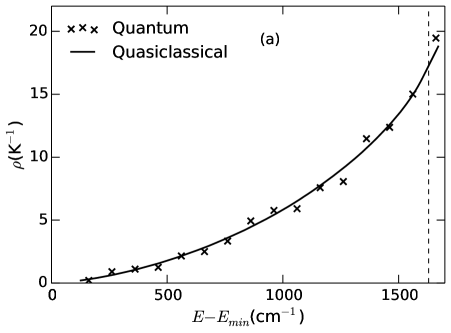
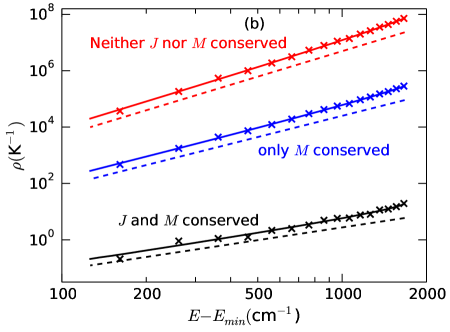
Figure 1: The DOS of K₂+Rb as a function of the energy, $E$, for quantum mechanical (crosses) and quasiclassical (solid line) calculations for an isotropic PES. In panel (a) this is shown for the field-free case on a linear scale, in panel (b) it is also plotted for the cases with fields on a double logarithmic scale. The vertical dashed line in panel (a) indicates the classical dissociation limit of the complex with $E-E_{\mathrm{min}}=D_{e}$. The dashed lines in panel (b) are straight lines with slopes 3, 2.5, and 1.5 and only serve to illustrate the power-law energy dependence of the DOS. Note that the crosses in the upper and lower graph are placed at the same energies.

In Fig. 1(a) we show the DOS as a function of the energy $E-E_{\mathrm{min}}$, where $E_{\mathrm{min}}$ is the energy of the minimum of the potential. The vertical dashed line indicates the classical dissociation limit for formation of Rb+K₂. Quantummechanically, the dissociation energy liest at slightly higher energy because of the zero-point energy of K₂. To compute the classical DOS we place the dividing surface at $R=R^{(0)}=20~{}a_{0}$. Above the classical dissociation limit the DOS keeps increasing when we move the dividing surface outwards, but only slowly.

The classical and quantum results agree closely with each other, especially below the classical dissociation limit. In the quantum case there are more fluctuations in the DOS, as expected. In Fig. 1(b) the DOSs are plotted on a double logarithmic scale, both for the case without field and with field(s). Again, the classical and quantum mechanical results agree very well. In the quantum case, the fluctuations become smaller as the DOS becomes larger.

The DOSs in 1(b) show a clear power-law dependence on the energy, $E$. Straight dashed lines with slopes from top to bottom 3, 2.5, and 1.5 are plotted alongside the DOSs to guide the eye. The integrand of Eq. (30) has exponent $1/2$, and when $J$ or $J$ and $M$ are not conserved these exponents become $3/2$ and 2, respectively. Here, we use an isotropic potential, which therefore does not depend on $\theta$. Each “harmonic” degree of freedom contributes $1/2$ to the exponent, such that the exponent would increase by one if the potentials as a function of $R$ and $r$ were perfectly harmonic. The slopes of the graphs are slightly higher near dissociation.

III.2 NaK-NaK

Next, we apply our method to the four-atom NaK-NaK system. We use the Jacobi coordinates $\bm{q}=(R,r_{1},r_{2},\theta_{1},\theta_{2},\phi)$, where $R$ is the NaK-NaK distance, $r_{1}$ and $r_{2}$ are the bond lengths, $\theta_{1}$ and $\theta_{2}$ the polar angles, and $\phi$ is the dihedral angle. In these coordinates, Eq. (27) for the general AB+CD DOS can be written as

$$\rho_{JMp}^{(\mathrm{AB}+\mathrm{CD})}(E)=\frac{g_{\bm{N}Jp}\,4\pi^{6}(2J+1)m_{\mathrm{A}}^{3}m_{\mathrm{B}}^{3}m_{C}^{3}m_{D}^{3}}{h^{9}(m_{\mathrm{A}}+m_{\mathrm{B}}+m_{\mathrm{C}}+m_{\mathrm{D}})^{3}g_{\mathrm{ABCD}}}\int\!\frac{R^{4}\,r_{1}^{4}\,r_{2}^{4}\sin^{2}(\theta_{1})\sin^{2}(\theta_{2})}{\det{\mathcal{I}(\bm{q})}\sqrt{\det{\mathcal{A}(\bm{q})}}}[E-V(\bm{q})]^{2}\,d\bm{q}.$$ (32)

Unlike for the three-atom system, there is no simple analytical expression for $\det{\mathcal{I}(\bm{q})}$ and $\det{\mathcal{A}(\bm{q})}$ for the four-atom system, so we calculated them numerically. For the NaK-NaK system, A and C are K, B and D are Na, and $g_{\bm{N}Jp}=1/2$. The expressions for $\mathcal{I}$ and $\bm{j}$ are given in appendix VI.2. In the quasiclassical calculations for the isotropic PES, we use an equidistant grid in $R$ from 5 to 20 $a_{0}$ with 151 points, a grid of $r_{1}$ from 4.5 to 10 $a_{0}$ with 56 points, a grid of $r_{2}$ ranging from $r_{1}$ to $10.5~{}a_{0}$ with a spacing of 0.1 $a_{0}$. We use a four-point Gauss-Legendre quadrature in $\theta_{1}$ and $\theta_{2}$ and a two-point Gauss-Chebyshev quadrature in $\phi$. We choose $r_{2}>r_{1}$ and multiply the result by a factor two because of the symmetry. An additional factor two is included to compensate for $\phi$ from running up to $\pi$ instead of $2\pi$.

The realistic potential energy surface of NaK-NaK consists of three parts Christianen et al. (2019): two symmetrically equivalent NaK-NaK parts and one Na₂-K₂ part. Although one set of Jacobi coordinates can in principle describe all arrangements, integrating over these Jacobi coordinates is very difficult, because an increasingly fine angular grid is needed when going further into an arrangement that does not match the chosen coordinates. We therefore construct a separate integration grid in Jacobi coordinates for all three arrangements and add the integrals. In the NaK-NaK arrangement for the realistic potential, we use an equidistant grid in $R$ with 31 points placed from 5 to 20 $a_{0}$. For $r_{1}$ we use a grid of 15 points from 4.5 to $9~{}a_{0}$, and for $r_{2}$ the grid ranges from $r_{1}$ to $10.5~{}a_{0}$, with a spacing of $0.3~{}a_{0}$. A 24-point Gauss-Legendre quadrature between 0 and $\pi$ is used for $\theta_{1}$ and $\theta_{2}$, and an 8-point Gauss-Chebyshev quadrature between 0 and $\pi$ is used for $\phi$. For the Na₂-K₂ we use a similar grid.

Because there are some overlapping parts of the grids in the center of the PES, we assign a geometry dependent weighting factor to the integrands for each arrangement. This weighting factor $W(\bm{q})$ is based on the symmetrization function in our previous work Christianen et al. (2019). In the NaK-NaK arrangements $W(\bm{q})=W_{1}W_{2}$ or $W(\bm{q})=W_{1}(1-W_{2})$, and in the Na₂-K₂ arrangement: $W(\bm{q})=1-W_{1}$, with

$$W(u,c,w)=\begin{cases}0,&\quad\text{if }u\leq c-w\\ \frac{1}{2}+\frac{9}{16}\sin{\frac{\pi(u-c)}{2w}}+\frac{1}{16}\sin{\frac{3\pi(u-c)}{2w}},&\quad\text{if }c-w<u<c+w\\ 1,&\quad\text{if }u\geq c+w.\end{cases}$$ (33)

We take $W_{1}\equiv W(u_{1},1,1/4)$ with

$$u_{1}=\frac{r_{12}+r_{34}}{2(r_{13}+r_{24})}+\frac{r_{12}+r_{34}}{2(r_{23}+r_{14})},$$ (34)

where $r_{ij}$ indicates the distance between atom $i$ and $j$. Atoms 1 and 2 are the K-atoms and atoms 3 and 4 are the Na-atoms and $W_{2}\equiv W(u_{2},1/2,1/16)$ with

$$u_{2}=\frac{r_{23}+r_{14}}{r_{13}+r_{24}+r_{23}+r_{14}}.$$ (35)

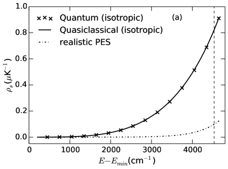
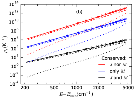
Figure 2: The DOS of NaK+NaK as a function of the energy, $E$, for quantum mechanical (crosses), quasiclassical (solid line) calculations for an isotropic PES and quasiclassical calculations for a realistic PES (dashed-dotted lines). Here $J=0$ and the quantum mechanical parity $p=1$. In panel (a) this is plotted only for the field-free case on a linear scale, in panel (b) it is also plotted for the cases with fields on a double logarithmic scale. The vertical dashed line in panel (a) indicates the classical dissociation enery of the complex, and the dashed lines in panel (b) are straight lines with slopes 5, 4.5, and 3.5 and only serve to illustrate the power-law energy dependence of the DOS.

Figure 2 shows the DOS for both the isotropic $r$-independent PES (quantum and quasiclassical) and for the realistic PES. For the isotropic PES, the NaK monomer potentials of Ref. Christianen et al. (2019) were used, together with a Lennard-Jones intermolecular potential with parameters $C_{6}=8500$ $E_{h}a_{0}^{6}$. and $D_{e}=4534$ cm^-1. First, we note that the quasiclassical-quantum correspondence is even better than in the case of K₂-Rb. This is not surprising given the DOS is larger by about five orders of magnitude at the dissociation energy. This results in fewer quantum fluctuations in the DOS. At the dissociation energy, the difference in DOS between the isotropic and realistic PESs is about one order of magnitude, both with and without angular momentum conservation. The slope of the DOS in Fig. 2(b) is much larger and less constant for the realistic PES than for the isotropic PES. This is due to anharmonicity and anisotropy of the PES. At the dissociation energy, the DOS for the realistic PES is found to be (for $J=0$): 0.124 $\mu$K^-1 in the field-free case, 2.14 nK^-1 if only $M$ is conserved, and 5.12 pK^-1 when neither $J$ nor $M$ is conserved. These DOS values correspond to RRKM sticking times of 5.96 $\mu$s, 103 ms, and 24.5 s, for these three cases, respectively.

III.3 Extrapolating the NaK-NaK results

In this section we estimate the DOS for other bialkali-bialkali systems by extrapolating the accurate DOS we obtained for NaK-NaK. To find approximate scaling laws, we use the values of $\det\mathcal{I}(\bm{y})$, $\det\mathcal{A}(\bm{y})$ in a planar, antiparallel configuration with the bond lengths $r_{1,2}$ at their equilibrium distances $r_{0}$ and the intermolecular distance $R$ at the minimum distance of the Lennard-Jones potential $R_{0}=(C_{6}/D_{e})^{1/6}$. We assume the potential is isotropic and harmonic, with the force constants $k_{R}=72D_{e}/R_{0}^{2}$ and $k_{r}=\omega^{2}m_{\mathrm{1}}m_{\mathrm{2}}/(m_{\mathrm{1}}+m_{\mathrm{2}})$, with $\omega$ the vibration frequency of the diatom. Furthermore, we consider only one arrangement, meaning we drop one factor $1/2$ for the symmetry. Substituting this into Eq. (32) yields an approximate DOS:

$$\tilde{\rho}(m_{1},m_{2},r_{0},D_{e},C_{6},\omega)=\frac{256\pi^{10}(2J+1)m_{1}^{5/2}m_{2}^{5/2}R_{0}r_{0}^{3}}{105h^{9}(m_{1}+m_{2})^{3/2}\sqrt{\frac{m_{1}+m_{2}}{2}R_{0}^{2}+2\frac{m_{1}m_{2}}{m_{1}+m_{2}}r_{0}^{2}}}\,\frac{1}{k_{r}\sqrt{k_{R}}}D_{e}^{\frac{7}{2}}C_{\mathrm{corr}}.$$ (36)

We use the DOS calculated using our realistic PES to determine the factor $C_{\mathrm{corr}}$ in the above expression, which is meant to correct for the anisotropy and anharmonicity of the PES. We find $C_{\mathrm{corr}}=0.23$. We fix the value of this correction factor, and subsequently evaluate Eq. (36) for all polar bialkali-bialkali systems. We use diatom properties from Ref. Fedorov et al. (2014), and $C_{6}$ coefficients and $D_{e}$ values from Ref. Byrd (2013). The resulting DOSs are listed listed in table 1. We see that—as expected from the equations—the DOS strongly increases when moving from lighter to heavier alkali systems. Here, the reduced mass plays a bigger role than the total mass, e.g., compare NaK to LiCs. We see that the sticking times of the collision complexes, in the absence of chemical reactions, change over three orders of magnitude when moving from 0.25 $\mu$s for NaLi, to 253 $\mu$s for RbCs. Note that for fermionic molecules, $s$-wave scattering is forbidden and that therefore $p$-wave scattering is the dominant mechanism. Therefore $J=1$ and the sticking time is increased by a factor $2J+1=3$, see Eq. (27).

Table 1: The estimated DOS, in $\mu$K^-1 (RRKM sticking time, in $\mu$s) for all singlet polar bialkali molecules ($J=0$) in a single hyperfine state. The star indicates the NaK-NaK sticking time has been determined accurately, without extrapolation.

	23Na	39K	87Rb	133Cs
7Li	0.0051 (0.25)	0.014 (0.67)	0.024 (1.17)	0.068 (3.3)
23Na	.	0.124(6.0)*	0.27 (12.9)	0.83 (40)
39K	.	.	0.48 (23.0)	1.50 (72)
87Rb	.	.	.	5.3 (253)

III.4 Sticking-amplified three-body loss

We use the calculated sticking times to study one particular loss mechanism that has been hypothesized to be responsible for the losses observed experimentally: sticking-amplified three-body loss. Here, a free diatom collides with a collision complex, leading to energy transfer from the complex to the diatom and the escape of both the complex and the diatom from the trap. To estimate the rate of this three-body loss process, we need to estimate the rate of complex-molecule collisions and compare the resulting lifetime to the sticking time of the complex.

The rate of complex-molecule collisions can be estimated with a quantum capture model Mayle et al. (2013). The only unknown parameter here is the dispersion ($C_{6}$) coefficient for complex-molecule collisions, which sets the mean scattering length and rate. This dispersion coefficient can be calculated from the dynamic dipole polarizabilities $\alpha(i\omega)$ at imaginary frequencies of both collision partners, A and B, using the Casimir-Polder relation,

$$C_{6}=\frac{3}{\pi}\int_{0}^{\infty}\alpha^{\mathrm{A}}(i\omega)\alpha^{\mathrm{B}}(i\omega)d\omega.$$ (37)

Quantum mechanically, the polarizability for a given state $i$ can be calculated from a sum over states, $f$, where $\omega_{fi}$ is the transition frequency

$$\alpha_{i}(i\omega)=\frac{2}{3}\sum_{f\neq i}\omega_{fi}\frac{|\langle f|\hat{\bm{\mu}}|i\rangle|^{2}}{\omega_{fi}^{2}+\omega^{2}}.$$ (38)

From Eq. (38) it is clear that the static dipole polarizability ($\omega=0$) is an upper limit for the polarizability. For a ground state molecule $\omega_{fi}$ is always positive. In the case of diatom-diatom collisions, the dispersion coefficient is mainly due to rotational dispersion Żuchowski et al. (2013) and $\alpha_{\mathrm{diatom}}(0)$ is given approximately by

$$\alpha_{\mathrm{diatom}}(0)=\frac{d^{2}}{3B},$$ (39)

where $B$ is the rotational constant and $d$ the dipole moment. The complex is clearly not in the ground state, meaning that terms of the sum in Eq. (38) in energy above and below the energy level of the complex could cancel to some extent, leading to a much smaller polarizability. Quasiclassically, this can be quantified for the static dipole polarizability. We derive in Appendix Sec. VI.3 that this static dipole polarizability can be expressed in terms of the following expectation value

$$\alpha_{\mathrm{complex}}(0)=\left\langle\frac{2d^{2}}{3T_{\mathrm{kin}}}\right\rangle_{\bm{q},\bm{\Omega}}.$$ (40)

Note that here $d$ is the total dipole moment of the complex, which depends on the geometry. This expression is remarkably similar to the expression for the free diatom. For the NaK-NaK system, the interaction energy can rise up to $4534$ cm^-1 Christianen et al. (2019). This means that the expectation value of $T_{\mathrm{kin}}$ is in the order of $10^{3}$ cm^-1, which is four orders of magnitude larger than the rotational constant of NaK, which is $0.095$ cm^-1. This means that the rotational dispersion contribution to the integral in Eq. (37), will be much smaller than in the diatom-diatom case. Therefore the electronic dispersion term is the most important contribution, which can be estimated to be twice the electronic dispersion coefficient for the diatom-diatom collisions. For NaK, this means that the dispersion coefficient for the complex-diatom collisions, will be $17\,000$ $E_{h}a_{0}^{6}$, which is an order of magnitude smaller than the value of $500\,000$ $E_{h}a_{0}^{6}$ for diatomic collisions, which may be counter-intuitive.

Using the multichannel quantum defect theory from Ref. Mayle et al. (2013) and taking the limit of $T\rightarrow 0$, this dispersion coefficient gives an $s$-wave rate coefficient of $1.1\cdot 10^{-10}$ cm³s^-1. Multiplying this by a typical density of the diatoms ($4\cdot 10^{10}$ cm^-3 Park et al. (2015)) and taking the inverse gives the lifetime of the complex due to three-body loss. This lifetime is given by $\tau_{3b}=0.23$ s. The sticking time of the NaK-NaK complex for $J=1$ is approximately $18~{}\mu s$, so the complex dissociates much faster than it collides with a third NaK diatom. Therefore, sticking-amplified three-body losses are not the cause of the losses in typical experimentsPark et al. (2015, 2017). Accounting solely for this loss mechanism, the lifetime of the NaK gas in the trap in the experimental conditions would be in the order of hoursPark et al. (2015, 2017). For the RbCs gas of Ref. Takekoshi et al. (2014) it would be tens of minutes. For the NaRb gas such as reported in Ref. Ye et al. (2018), the loss would be on the timescale of a minute, due to the relatively high densities.

The conclusion that three-body collisions are not the cause the experimental losses is based on the sticking time without fields and without taking into account hyperfine transitions. The conclusion may change in the presence of strong electric or magnetic fields, which cause $J$ to no longer be conserved. However, it is not clear from our calculations how strong the external fields need to be to affect the DOS. The DOS, and therefore the sticking time, can also strongly increase in case of hyperfine transitions of the collision complex. However, it is not directly clear whether these occur on the timescale of the sticking time, especially since there are no unpaired electronic spins and the hyperfine transitions must therefore be caused by coupling to the rotational states. The strongest hyperfine coupling is due to the nuclear quadrupole moments interacting with the changing electric field gradients during the collisions. Both the inclusion of hyperfine states into the model or $J$ not being conserved may cause the sticking times to be orders of magnitude larger and may cause the three-body collision mechanism to be more important.

IV Conclusion and discussion

We have derived a quasiclassical equation for the DOS of an ultracold, $N$-atom collision complex, for an arbitrary PES [Eq. (27)]. We have established the accuracy of our quasiclassical method by comparing to exact quantum results for the K₂-Rb and NaK-NaK system, with isotropic $r$-independent model PESs. We have calculated the DOS for an accurate NaK-NaK PES to be 0.124 $\mu$K^-1, with an associated RRKM sticking time of 5.96 $\mu$s. We extrapolate our results to the other bialkali-bialkali systems. The resulting DOS increases rapidly with atomic mass, but only up to 5 $\mu$K^-1 for the heaviest system RbCs, two orders of magnitude below what was reported previously Mayle et al. (2013). Using the resulting sticking times, we conclude a sticking-amplified three-body loss mechanism is not the cause of losses in the experiments.

V Acknowledgements

We thank James Croft and John Bohn for valuable discussions and Dongzheng Yang for carefully checking all derivations in the manuscript. T.K. is supported by NWO Rubicon grant 019.172EN.007 and an NSF grant to ITAMP.

VI Appendix

VI.1 DOS in presence of a field

We are interested in the DOS in the presence of, e.g., an electric field, where $J$ is no longer conserved, but $M$ still is. For the DOS calculation this means that we can no longer treat space isotropically and neglect the $J$-dependence of the kinetic energy. We modify Eq. (25) accordingly, resulting in

$$N=\frac{C_{\bm{Nm}}}{\Gamma(\frac{D}{2}+1)}\int\!d\bm{q}\int\!d\bm{\Omega}\sin(\beta)\int\!d\bm{J}\,G(\bm{q})\left\{\pi\left[E-V(\bm{q})-\frac{\bm{J}^{T}\mathcal{R}(\bm{\Omega})[\mathcal{I}(\bm{q})^{-1}]^{(\mathrm{bf})}\mathcal{R}(\bm{\Omega})^{-1}\bm{J}}{2}\right]\right\}^{\frac{D}{2}}.$$ (41)

For conserved $M=0$, we integrate over $J_{z}$ from $-1/2$ to $1/2$. This is inaccurate only for the $J=0$ state, but the contribution of $J=0$ to the total DOS is very small if all $J$ are accessible. Because $M_{z}=0$ we can neglect the kinetic energy associated with $J_{z}$, so

$$N=\frac{2C_{\bm{Nm}}}{\Gamma(\frac{D}{2}+2)}\int\!d\bm{q}\int\!d\bm{\Omega}\sin(\beta)\frac{G(\bm{q})}{\sqrt{M_{zz}}}\\ \left\{\pi\left[E-V(\bm{q})\right]\right\}^{\frac{D}{2}+1},$$ (42)

where $M_{zz}$ is the minor of the $z,z$ element of $\mathcal{R}(\bm{\Omega})^{-1}\mathcal{I}(\bm{q})^{-1}\mathcal{R}(\bm{\Omega})$. By Cramer’s rule the minor $M_{zz}$ of a matrix ${\mathcal{X}}$ is equal to $({\mathcal{X}}^{-1})_{zz}\det{\mathcal{X}}$, so

$$\frac{1}{\sqrt{M_{zz}}}=\frac{\det\mathcal{I}(\bm{q})}{\sqrt{[\mathcal{R}(\bm{\Omega})^{-1}\mathcal{I}(\bm{q})\mathcal{R}(\bm{\Omega}]_{zz}}}.$$ (43)

The denominator in this expression depends only on the first two Euler angles $\alpha$ and $\beta$ and we find

$$N=\frac{4\pi C_{\bm{Nm}}}{\Gamma(\frac{D}{2}+2)}\int\!d\bm{q}\,G(\bm{q})\sqrt{\det{\mathcal{I}(\bm{q})}}\left\{\pi\left[E-V(\bm{q})\right]\right\}^{\frac{D}{2}+1}\\ \int_{0}^{2\pi}\!d\alpha\int_{0}^{\pi}\!d\beta\frac{\sin(\beta)}{\sqrt{\mathcal{I}_{1}(\bm{q})\cos^{2}(\beta)+\mathcal{I}_{2}(\bm{q})\sin^{2}(\beta)\cos^{2}(\alpha)+\mathcal{I}_{3}(\bm{q})\sin^{2}(\beta)\sin^{2}(\alpha)}},$$ (44)

where we have chosen the lower integration bound, the zeroes of $\bm{\Omega}$, such that the inertial tensor is diagonal and the eigenvalues are ordered in magnitude. The variables $\mathcal{I}_{1}(\bm{q})$, $\mathcal{I}_{2}(\bm{q})$, and $\mathcal{I}_{3}(\bm{q})$ are the eigenvalues of $\mathcal{I}(\bm{q})$, where $\mathcal{I}_{1}(\bm{q})$ is the largest and $\mathcal{I}_{3}(\bm{q})$ the smallest. This choice is possible since we integrate over all angles, such that the integral is independent of the starting point.

The integral over $\beta$ results in

$$\frac{4\pi}{\sqrt{\mathcal{I}}_{\mathrm{rot}}}=\frac{1}{\sqrt{\mathcal{I}_{1}}}\int_{0}^{2\pi}\!d\alpha\,\frac{\{\log[1+f(\alpha)]-\log[1-f(\alpha)]\}}{f(\alpha)},$$ (45)

where

$$f(\alpha)=\sqrt{1-\frac{\mathcal{I}_{2}\cos^{2}(\alpha)+\mathcal{I}_{3}\sin^{2}(\alpha)}{\mathcal{I}_{1}}},$$ (46)

and $\mathcal{I}_{\mathrm{rot}}$ is the “rotationally averaged” value of $\mathcal{I}_{zz}$. An analytical expression for this integral can be obtained by expanding the logarithms as a power series. Only even powers of $f(\alpha)$ remain and all resulting integrals can be calculated analytically, yielding

$$\frac{4\pi}{\sqrt{\mathcal{I}}_{\mathrm{rot}}} =\frac{2}{\sqrt{\mathcal{I}_{1}}}\sum_{n=0}^{\infty}\frac{1}{2n+1}\int_{0}^{2\pi}\left[(1-\frac{\mathcal{I}_{3}}{\mathcal{I}_{1}})-(\frac{\mathcal{I}_{2}-\mathcal{I}_{3}}{\mathcal{I}_{1}})\cos^{2}(\alpha)\right]^{n}d\alpha$$ (47)

$$=\frac{4\pi}{\sqrt{\mathcal{I}_{1}}}\sum_{n=0}^{\infty}\frac{\left(1-\frac{\mathcal{I}_{3}}{\mathcal{I}_{1}}\right)^{n}}{2n+1}{}_{2}F_{1}\left(\frac{1}{2},-n;1;\frac{\mathcal{I}_{2}-\mathcal{I}_{3}}{\mathcal{I}_{1}-\mathcal{I}_{3}}\right),$$ (48)

where ${}_{2}F_{1}{}$ is the hypergeometric function. The sum converges rapidly as long as ${\mathcal{I}_{3}}$ is of the same order as $\mathcal{I}_{1}$ and $\mathcal{I}_{2}$. The values this sum can assume lie between $1$ and $\pi/2$. If we substitute this result into Eq. (44), we obtain

$$N=\frac{16\pi^{2}C_{\bm{Nm}}}{\Gamma(\frac{D}{2}+2)}\int\!d\bm{q}\,G(\bm{q})\sqrt{\frac{\det\mathcal{I}(\bm{q})}{\mathcal{I}_{\mathrm{rot}}(\bm{q})}}\{\pi[E-V(\bm{q})]\}^{\frac{D}{2}+1},$$ (49)

and

$$\rho=\frac{16\pi^{3}C_{\bm{Nm}}}{\Gamma(\frac{D}{2}+1)}\int\!d\bm{q}\,G(\bm{q})\sqrt{\frac{\det\mathcal{I}(\bm{q})}{\mathcal{I}_{\mathrm{rot}}(\bm{q})}}\{\pi[E-V(\bm{q})]\}^{\frac{D}{2}}.$$ (50)

VI.2 Example calculations for K₂-Rb and NaK-NaK

For K₂-Rb the kinetic energy (for $J=0$) can be written as:

$$E_{kin}=\frac{\mu_{K_{2}Rb}}{2}\dot{R}^{2}+\frac{m_{\mathrm{K}}}{4}\dot{r}^{2}+\frac{m_{\mathrm{K}}}{4}r^{2}\dot{\theta}^{2}-\frac{\bm{j}^{T}\mathcal{I}^{-1}\bm{j}}{2}.$$ (51)

If we define the $\bm{x}^{\mathrm{(bf)}}$ coordinates by choosing the K₂ molecule to be in the $xy$-plane and the $R$ to be along the $x$-axis, then $\bm{j}$ is given by

$$\bm{j}=\begin{pmatrix}0\\ 0\\ \frac{m_{\mathrm{K}}}{2}r^{2}\dot{\theta}\end{pmatrix},$$ (52)

and $\mathcal{I}$ is given by

$$\mathcal{I}_{xx} =\frac{m_{\mathrm{K}}}{2}r^{2}\sin^{2}(\theta),$$

$$\mathcal{I}_{yy} =\frac{m_{\mathrm{K}}}{2}r^{2}\cos^{2}(\theta)+\mu_{K_{2}Rb}R^{2},$$

$$\mathcal{I}_{zz} =\frac{m_{\mathrm{K}}}{2}r^{2}+\mu_{K_{2}Rb}R^{2},$$

$$\mathcal{I}_{xy} =\mathcal{I}_{yx}=-\frac{m_{\mathrm{K}}}{2}r^{2}\cos(\theta)\sin(\theta),$$

$$\mathcal{I}_{xz} =\mathcal{I}_{zx}=0,$$

$$\mathcal{I}_{yz} =\mathcal{I}_{zy}=0.$$

For the NaK-NaK system, the kinetic energy (for $J=0$) can be written as

$$T_{\mathrm{kin}}=\frac{\mu_{\mathrm{NaK}}}{2}\left[\dot{r}_{1}^{2}+\dot{r}_{2}^{2}+r_{1}^{2}\dot{\theta}_{1}^{2}+r_{2}^{2}\dot{\theta}_{2}^{2}+r_{2}^{2}\sin^{2}(\theta_{2})\dot{\phi}^{2}\right]+\frac{m_{\mathrm{Na}}+m_{\mathrm{K}}}{4}\dot{R}^{2}-\frac{\bm{j}^{T}\mathcal{I}^{-1}\bm{j}}{2}.$$ (53)

If we choose $r_{1}$ and $R$ to lie in the $xy$-plane, with $R$ along the $x$-axis, then $\bm{j}$ is given by

$$\bm{j}=\begin{pmatrix}\mu_{\mathrm{NaK}}r_{2}^{2}\sin^{2}(\theta_{2})\dot{\phi}\\ -\mu_{\mathrm{NaK}}[r_{2}^{2}\sin(\phi)\dot{\theta_{2}}+r_{2}^{2}\sin(\theta_{2})\cos(\theta_{2})\cos(\phi)\dot{\phi}]\\ \mu_{\mathrm{NaK}}[r_{1}^{2}\dot{\theta_{1}}+r_{2}^{2}\cos(\phi)\dot{\theta_{2}}-r_{2}^{2}\sin(\theta_{2})\cos(\theta_{2})\sin(\phi)\dot{\phi}]\end{pmatrix}.$$ (54)

For the elements of $\mathcal{I}$ we find

$$\mathcal{I}_{xx} =\mu_{\mathrm{NaK}}[r_{1}^{2}\sin^{2}(\theta_{1})+r_{2}^{2}\sin^{2}(\theta_{2})],$$

$$\mathcal{I}_{yy} =\mu_{\mathrm{NaK}}[r_{1}^{2}\cos^{2}(\theta_{1})+r_{2}^{2}\cos^{2}(\theta_{2})+r_{2}^{2}\sin^{2}(\theta_{2})\sin^{2}(\phi)]+\frac{m_{\mathrm{K}}+m_{\mathrm{Na}}}{2}R^{2},$$

$$\mathcal{I}_{zz} =\mu_{\mathrm{NaK}}[r_{1}^{2}+r_{2}^{2}\cos^{2}(\theta_{2})+r_{2}^{2}\sin^{2}(\theta_{2})\cos^{2}(\phi)]+\frac{m_{\mathrm{K}}+m_{\mathrm{Na}}}{2}R^{2},$$

$$\mathcal{I}_{xy} =\mathcal{I}_{yx}=-\mu_{\mathrm{NaK}}[r_{1}^{2}\cos(\theta_{1})\sin(\theta_{1})+r_{2}^{2}\cos(\theta_{2})\sin(\theta_{2})\cos(\phi)],$$

$$\mathcal{I}_{xz} =\mathcal{I}_{zx}=-\mu_{\mathrm{NaK}}r_{2}^{2}\cos(\theta_{2})\sin(\theta_{2})\sin(\phi),$$

$$\mathcal{I}_{yz} =\mathcal{I}_{zy}=-\mu_{\mathrm{NaK}}r_{2}^{2}\sin^{2}(\theta_{2})\sin(\phi)\cos(\phi).$$

VI.3 Polarizability of a complex

In Sec. III.4 we argue qualitatively that the static dipole polarizability of the complex is much smaller than for the diatoms. Here we use our quasiclassical formalism to express the polarizability as an expectation value over phase space. For the complex, we can calculate the expectation value of the static dipole polarizability in our quasiclassical framework. If we re-introduce the integral over the Euler angles $\bm{\Omega}$ in Eq. (27) and introduce an external field $\bm{F}$, we can write the DOS as

$$\rho(\bm{F})=\int d\bm{q}\,d\bm{\Omega}\,\sin(\beta)\,\delta\rho(\bm{q},\bm{\Omega},\bm{F}),$$ (55)

where $\delta\rho(\bm{q},\bm{\Omega})$ is given by

$$\delta\rho(\bm{q},\bm{\Omega},\bm{F})=\frac{g_{\bm{N}Jp}\pi^{1+\frac{D}{2}}\hbar^{3}C_{\bm{Nm}}(2J+1)}{\Gamma(\frac{D}{2})}G(\bm{q})[E-V(\bm{q})-f(\bm{q},\bm{\Omega},\bm{F})]^{\frac{D}{2}-1}.$$ (56)

Here $f(\bm{q},\bm{\Omega},\bm{F})$ is a perturbation on the energy caused by the external field $\bm{F}$, which we assume to be small enough for $\mathcal{J}$ to still be (approximately) conserved. Then the expectation of $\chi(\bm{q},\bm{\Omega})$ can be calculated as

$$\langle\chi\rangle_{\bm{q},\bm{\Omega}}(\bm{F})=\frac{1}{\rho}\int\!d\bm{q}\,d\bm{\Omega}\,\sin(\beta)\,\delta\rho(\bm{q},\bm{\Omega},\bm{F})\,\chi(\bm{q},\bm{\Omega},\bm{F}).$$ (57)

The polarizability tensor $\alpha$ is given by

$$\alpha_{ij}=\frac{\partial d_{i}}{\partial\mathcal{E}_{j}},$$ (58)

where $\bm{\mathcal{E}}$ is the electric field and $\bm{d}(\bm{q},\bm{\Omega})$ the electric dipole moment. The electric dipole moment is given by the vector sum of the dipoles of the two NaK molecules. These molecular dipoles lie along the molecular axes, the directions of which depend on $\bm{q}$ and $\bm{\Omega}$.

The interaction energy of the system with an electric field is given by $-\bm{d}\cdot\bm{\mathcal{E}}$. The expectation value of the electric dipole moment, for a given $J$, is given by

$$\langle d_{i}\rangle_{\bm{q},\bm{\Omega}}(\bm{\mathcal{E}})=\frac{g_{\bm{N}Jp}\pi^{1+\frac{D}{2}}\hbar^{3}C_{\bm{Nm}}(2J+1)}{\Gamma(\frac{D}{2})\rho}\int\!d\bm{q}\,d\bm{\Omega}\,\sin(\beta)\,G(\bm{q})[E-V(\bm{q})+\bm{d}(\bm{q},\bm{\Omega})\cdot\bm{\mathcal{E}}]^{\frac{D}{2}-1}d_{i}(\bm{q},\bm{\Omega}).$$ (59)

Because of the integration over $\bm{\Omega}$, the expectation value of the dipole moment in the weak field limit vanishes. For the polarizability, the off-diagonal components integrate to zero, but the diagonal components do not. The expectation values of the diagonal polarizability components (if we take $\bm{\mathcal{E}}=0$) are given by

$$\langle\alpha_{ii}\rangle_{\bm{q},\bm{\Omega}}=\frac{g_{\bm{N}Jp}\pi^{1+\frac{D}{2}}\hbar^{3}C_{\bm{Nm}}(2J+1)}{\Gamma(\frac{D}{2}-1)\rho}\int\!d\bm{q}\,d\bm{\Omega}\,\sin(\beta)\,G(\bm{q})[E-V(\bm{q})]^{\frac{D}{2}-2}d_{i}(\bm{q},\bm{\Omega})^{2}.$$ (60)

If we introduce the isotropic polarizability as $\alpha_{0}=\frac{1}{3}(\alpha_{xx}+\alpha_{yy}+\alpha_{zz})$, we obtain

$$\langle\alpha_{0}\rangle_{\bm{q},\bm{\Omega}}=\frac{g_{\bm{N}Jp}\pi^{1+\frac{D}{2}}\hbar^{3}C_{\bm{Nm}}(2J+1)}{3\Gamma(\frac{D}{2}-1)}\int\!d\bm{q}\,d\bm{\Omega}\,\sin(\beta)\,G(\bm{q})[E-V(\bm{q})]^{\frac{D}{2}-2}d(\bm{q})^{2}.$$ (61)

Comparing to Eq. (57), this expression can be written as

$$\langle\alpha_{0}\rangle_{\bm{q},\bm{\Omega}}=\frac{\frac{D}{2}-1}{3\rho}\int\!d\bm{q}\,d\bm{\Omega}\,\sin(\beta)\frac{\delta\rho(\bm{q},\bm{\Omega},0)d(\bm{q})^{2}}{E-V(\bm{q})}=\frac{\frac{D}{2}-1}{3}\left\langle\frac{d^{2}}{T_{\mathrm{kin}}}\right\rangle_{\bm{q},\bm{\Omega}}.$$ (62)

For a diatom-diatom complex $D=6$ and therefore the static dipole polarizability becomes

$$\alpha_{0}=\left\langle\frac{2d^{2}}{3T_{\mathrm{kin}}}\right\rangle_{\bm{q},\bm{\Omega}}.$$ (63)

References

- DeMille (2002) D. DeMille, Phys. Rev. Lett. 88, 067901 (2002).
- Yelin et al. (2006) S. F. Yelin, K. Kirby, and R. Côté, Phys. Rev. A 74, 050301 (2006).
- Ni et al. (2018) K.-K. Ni, T. Rosenband, and D. D. Grimes, Chem. Sci. 9, 6830 (2018).
- Micheli et al. (2006) A. Micheli, G. K. Brennen, and P. Zoller, Nat. Phys. 2, 341 (2006).
- Büchler et al. (2007) H. P. Büchler, E. Demler, M. Lukin, A. Micheli, N. Prokof’ev, G. Pupillo, and P. Zoller, Phys. Rev. Lett. 98, 060404 (2007).
- Cooper and Shlyapnikov (2009) N. R. Cooper and G. V. Shlyapnikov, Phys. Rev. Lett. 103, 155302 (2009).
- Krems (2008) R. V. Krems, Phys. Chem. Chem. Phys. 10, 4079 (2008).
- Ospelkaus et al. (2010) S. Ospelkaus, K.-K. Ni, D. Wang, M. H. G. de Miranda, B. Neyenhuis, G. Quéméner, P. S. Julienne, J. L. Bohn, D. S. Jin, and J. Ye, Science 327, 853 (2010).
- Andreev et al. (2018) V. Andreev, D. G. Ang, D. DeMille, J. M. Doyle, G. Gabrielse, J. Haefner, N. R. Hutzler, Z. Lasner, C. Meisenhelder, B. R. O’Leary, C. D. Panda, A. D. West, E. P. West, and X. A. C. Wu, Nature 562, 355 (2018).
- Takekoshi et al. (2014) T. Takekoshi, L. Reichsöllner, A. Schindewolf, J. M. Hutson, C. R. L. Sueur, O. Dulieu, F. Ferlaino, R. Grimm, and H.-C. Nägerl, Phys. Rev. Lett. 113, 205301 (2014).
- Molony et al. (2014) P. K. Molony, P. D. Gregory, Z. Ji, B. Lu, M. P. Köppinger, C. R. L. Sueur, C. L. Blackley, J. M. Hutson, and S. L. Cornish, Phys. Rev. Lett. 113, 255301 (2014).
- Guo et al. (2016) M. Guo, B. Zhu, B. Lu, X. Ye, F. Wang, R. Vexiau, N. Bouloufa-Maafa, G. Quéméner, O. Dulieu, and D. Wang, Phys. Rev. Lett. 116, 205303 (2016).
- Park et al. (2015) J. W. Park, S. A. Will, and M. W. Zwierlein, Phys. Rev. Lett. 114, 205302 (2015).
- Seeßelberg et al. (2018) F. Seeßelberg, N. Buchheim, Z.-K. Lu, T. Schneider, X.-Y. Luo, E. Tiemann, I. Bloch, and C. Gohle, Phys. Rev. A 97, 013405 (2018).
- Park et al. (2017) J. W. Park, Z. Z. Yan, H. Loh, S. A. Will, and M. W. Zwierlein, Science 357, 372 (2017).
- Ye et al. (2018) X. Ye, M. Guo, M. L. González-Martínez, G. Quéméner, and D. Wang, Sci. Adv. 4 (2018).
- Quéméner and Julienne (2012) G. Quéméner and P. S. Julienne, Chem. Rev. 112, 4949 (2012).
- Mayle et al. (2013) M. Mayle, G. Quéméner, B. P. Ruzic, and J. L. Bohn, Phys. Rev. A 87, 012709 (2013).
- Gregory et al. (2019) P. D. Gregory, M. D. Frye, J. A. Blackmore, E. M. Bridge, R. Sawant, J. M. Hutson, and S. L. Cornish, preprint arXiv:1904.00654 (2019).
- F. E. Croft et al. (2017) J. F. E. Croft, N. Balakrishnan, and B. K. Kendrick, Phys. Rev. A 96, 062707 (2017).
- Mayle et al. (2012) M. Mayle, B. P. Ruzic, and J. L. Bohn, Phys. Rev. A 85, 062712 (2012).
- Levine (2005) R. D. Levine, Molecular Reaction Dynamics (Cambridge University Press, 2005).
- Croft et al. (2017) J. F. E. Croft, C. Makrides, M. Li, A. Petrov, B. K. Kendrick, N. Balakrishnan, and S. Kotochigova, Nat. Comm. 8, 15897 (2017).
- Christianen et al. (2019) A. Christianen, T. Karman, R. A. Vargas-Hernández, G. C. Groenenboom, and R. V. Krems, J. Chem. Phys. 150, 064106 (2019).
- Peslherbe and Hase (1994) G. H. Peslherbe and W. L. Hase, J. Chem. Phys. 101, 8535 (1994).
- Fedorov et al. (2014) D. A. Fedorov, A. Derevianko, and S. A. Varganov, J. Chem. Phys. 140, 184315 (2014).
- Byrd (2013) J. Byrd, Ultracold Chemistry of Alkali Clusters, Ph.D. thesis, University of Connecticut (2013).
- Żuchowski et al. (2013) P. S. Żuchowski, M. Kosicki, M. Kodrycka, and P. Soldán, Phys. Rev. A 87, 022706 (2013).