Driving an electrolyte through a corrugated nanopore

Abstract

We characterize the dynamics of a $z-z$ electrolyte embedded in a varying-section channel. In the linear response regime, by means of suitable approximations, we derive the Onsager matrix associated to externally enforced gradients in electrostatic potential, chemical potential, and pressure, for both dielectric and conducting channel walls. We show here that the linear transport coefficients are particularly sensitive to the geometry and the conductive properties of the channel walls when the Debye length is comparable to the channel width.In this regime, we found that one pair of off-diagonal Onsager matrix elements increases with the corrugation of the channel transport, in contrast to all other elements which are either unaffected by or decrease with increasing corrugation. Our results have a possible impact on the design of blue-energy devices as well as on the understanding of biological ion channels through membranes

I Introduction

Many biological systems Alberts et al. (2007) and synthetic devices Bocquet and Charlaix (2010) rely on the dynamics of electrolytes confined within micro- and nano-pores. For example, ion channels Calero et al. (2011); Peyser et al. (2014), membranes Melnikov et al. (2017); Bacchin (2018), neuron signaling Alberts et al. (2007), plant circulation Wheeler and Stroock (2008), and lymphatic Nipper and Dixon (2011) and interstitial Wiig and Swartz (2012) systems rely on the transport of electrolytes across tortuous micro- and nano-pores. Recent technological advances have lead to the realization of nanotubes and nanopores of controllable shape Siria et al. (2013); Secchi et al. (2016) that have been exploited to separate DNA, proteins Bonthuis et al. (2008), or colloids Dubov et al. (2017). Likewise, resistive-pulse sensing techniques have been developed to measure properties of tracers transported across charged nanopores Saleh and Sohn (2003); Ito et al. (2004); Heins et al. (2005); Arjmandi et al. (2012). Moreover, electrolyte-immersed electrodes have been characterized Šamaj and Trizac (2016); Reindl et al. (2017a, b) and realized for novel energy-harvesting devices Brogioli (2009). Recently it has been shown that novel dynamical regimes appear when the section of the confining vessel is not constant. Indeed, asymmetric pores have been used to pump Yeh et al. (2015) and to rectify ionic currents Siwy et al. (2005); Kosinska et al. (2008); Gomez et al. (2015); Laohakunakorn and Keyser (2015); Lairez et al. (2016). Moreover, recirculation has been reported for electrolytes confined between corrugated walls Park et al. (2006); Mani et al. (2009); Malgaretti et al. (2014); Chinappi and Malgaretti (2018), and the variation in the section of the channels can tune their permeability Malgaretti et al. (2015, 2016). When an electrolyte is driven inside such conduits the local variations in the available space will couple to the local charge and ionic density distribution leading to modulations in the mesoscopic properties of the electrolyte such as the electrostatic decay length.

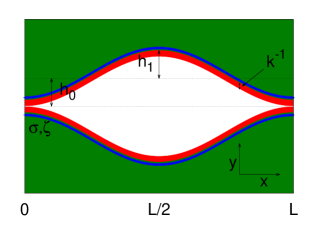
Figure 1: Schematic view of the system. The green regions are the channel walls, the red stripe represents the region, of size Debye length, where the electrostatic potential decays and the blue stripes represent the channel walls.

In this article, we show that analytical insight into such corrections can be obtained for smoothly–varying channel sections. In this scenario, we exploit the lubrication approximation and we derive closed expressions for the geometrically–induced corrections to the local electrostatic potential, charge, and ionic density distributions and we identify the fluxes driven by weak external driving forces through applied electric fields, pressure, or salt concentration differences for both conducting and dielectric channel walls. While for constant section channels the transpo coefficents are unaffected by the wall properties, for varying section channels , we show that the transport coefficeints are generally larger for dielectric walls. Moreover, upon increasing the corrugation of the channel we show that, as expected, the transport coefficients generally decrease. However, for some specific cases we find an increase of the transport coefficients upon increasing the corrugation of the channel.

The structure of the text is as follows. In section II we introduce our model setup and the framework of electrokinetic equations that we use to describe solute and solvent fluxes. In section III we determine the reference equilibrium scenario. In section IV we derive the linear transport coefficients of a channel driven out of equilibrium and show that the corresponding Onsager matrix is symmetric. The Onsager matrix encodes for many physical scenarios of possible experimental interest. We discuss several of those scenarios in section V. Finally, in section VII we present our conclusions.

II Model

II.1 Setup

Throughout this article, we analyze a microfluidic channel filled with a $z-z$ electrolyte in a solvent of dielectric constant $\epsilon$. The solvent is incompressible and has a viscosity $\eta$. The channel of length $L$ along the $x$-direction is translationally invariant in the $z$-direction and has a varying pore width in the $y$-direction: the channel half section $h(x)$ depends solely on $x$. We write $\bar{h}\equiv(1/L)\int_{0}^{L}h(x)\,\mathrm{d}x$ for the average pore section.

At $x=0$ and $x=L$, the channel is in contact with two chemostats at electrochemical potentials $\mu^{\pm}(x=0)$ and $\mu^{\pm}(x=L)$, respectively. Next to differences in these chemical potentials on either side of the channel, also a pressure difference $\Delta P$ or a potential difference $\Delta V$ can be applied. We only consider isothermal systems at temperature $T$, which means that local heat generation Janssen et al. (2017) is neglected. Moreover, our model does not account for surface conduction in the Stern layer Werkhoven et al. (2018).

II.2 Electrokinetic equations

Under the above described conditions, the steady state of our system can be modeled by the classical electrokinetic equations:

$$\epsilon\nabla^{2}\psi(x,y) =-zeq(x,y)\,,$$ (1a)

$$\textbf{j}^{\pm}(x,y) =\rho^{\pm}(x,y)\left[\textbf{v}(x,y)-D\beta\bm{\nabla}\mu^{\pm}(x,y)\right]\,,$$ (1b)

$$\bm{\nabla}\cdot\textbf{j}^{\pm}(x,y) =0\,,$$ (1c)

$$\eta\nabla^{2}\textbf{v}(x,y) =-\textbf{F}_{\text{tot}}(x,y)+\bm{\nabla}P_{\text{tot}}(x)\,,$$ (1d)

$$\bm{\nabla}\cdot\textbf{v}(x,y) =0\,.$$ (1e)

First, the electrostatic potential $\psi$ inside the channel is determined by the Poisson equation (1a) with $e$ being the elementary charge and with $q(x,y)$ being the local charge number density (m^-3), which is nonzero whenever there is a difference between cationic and anionic number densities ($\rho^{+}$ and $\rho^{-}$, respectively),

$$q(x,y)=\rho^{+}(x,y)-\rho^{-}(x,y)\,.$$ (2)

Second, we model the ionic currents $\textbf{j}^{\pm}$ by the Nernst-Planck equation (1b), which accounts for ionic transport by advection, diffusion, and electromigration. Equation (1b) describes the dynamics of point-like ions: this represents a fair approximation for dilute electrolytes in small electric fields. Third, when the system is driven by an external force such as a pressure drop or an electrostatic field, the electrolyte solution will flow —at low Reynolds number— according to the Stokes equation (1d), with $\partial_{x}P_{\text{tot}}(x)=\partial_{x}P(x)+\Delta P/L$, where $\partial_{x}P$ is the $x$-component of the geometrically-induced local pressure gradient that is determined by the boundary conditions and by fluid incompressibility and where

$$F_{\text{tot}}(x,y)=-zeq(x,y)\partial_{x}\psi(x,y)$$ (3)

is the $x$-component of the total electrostatic force density acting on the fluid. Finally, Eqs. (1c) and (1e) represent the steady-state continuity equation and the incompressibility equation, respectively.

Equations (1) are subject to the following boundary conditions

$$\psi\to\begin{cases}\psi(x,\pm h(x))&=\zeta\quad\quad\text{cond}\,,\\ \mathbf{n}^{\pm}\cdot\nabla\psi(x,y)|_{y=\pm h(x)}&=\pm e\sigma\quad\text{diel}\,,\end{cases}$$ (4a)

$$\mathbf{n}^{\pm}\cdot\mathbf{j}^{\pm}(x,\pm h(x))=0\,,$$ (4b)

$$\textbf{v}(x,\pm h(x))=0\,,$$ (4c)

where $\mathbf{n}^{\pm}$ is the local normal at the channel walls. Here, the boundary conditions on $\psi(x,y)$ depend on the conductive properties of the channel walls. For dielectric channel walls, the case for pores made from polymeric materials such as PDMS, we impose a constant surface charge $e\sigma$ whereas for conducting walls, such as carbon nanotubes, we impose a constant $\zeta$ potential. We denote the electrostatic potential in either case $\psi^{\zeta}(x,y)$ or $\psi^{\sigma}(x,y)$, accordingly. Note that while for flat channels either choices are related via the capacitance, in the corrugated case, a constant $\zeta$ potential leads to a $x$-dependent surface charge $e\sigma(x)$ [cf. Eq. (17)], while a constant surface charge gives rise to a varying surface potential $\psi^{\sigma}(x,h(x))$ [cf. Eq. (14)]. The same superscript notation is also used for other variables whenever we specify quantities to either boundary conditions. Equations (4b) and (4c) represent the no-flux and no-slip boundary conditions at the channel walls of the solute and solvent, respectively.

II.3 Lubrication approximation

In the following we restrict to pores whose section vary smoothly. This allows us to identify a separation between longitudinal and transverse length scales according to which changes of $\psi$ and $v_{x}$ along the $x$-direction are much smaller than those along the $y$-direction. This facilitates an essential simplification of Eqs. (1a) and (1d) where $\partial_{x}^{2}$ terms therein become negligible as compared to $\partial_{y}^{2}$ terms. Thanks to this “lubrication-like” approximation both Eq. (1a) and Eq. (1d) become analytically solvable. In order to apply the lubrication approximation consistently to both the Stokes and Poisson equation, we need to identify a common small parameter. While the relevant longitudinal length scale of both the Stokes equation and the Poisson equation is the channel length $L$, different transverse length scales appear in these equations: the average channel section $\bar{h}$, for the Stokes equation, and the screening length $\lambda$, for the Poisson equation. To proceed, we nondimensionalize the length scales via: $x=x_{*}L$ and $h(x)=h_{*}(x)\bar{h}$, while for the transverse direction we use either $y=y_{*}\bar{h}$ or $y=y_{\star}\lambda$. We then write the Stokes equation as

$$\frac{\bar{h}^{2}}{L^{2}}\frac{\partial^{2}v_{x}}{\partial x_{*}^{2}}+\frac{\partial^{2}v_{x}}{\partial y_{*}^{2}}=\frac{\bar{h}^{2}}{\eta}\left[-F_{\text{tot}}(x,y)+\partial_{x}P_{\text{tot}}(x)\right]\,,$$ (5)

and the Poisson equation as

$$\frac{\lambda^{2}}{\bar{h}^{2}}\frac{\bar{h}^{2}}{L^{2}}\left[\frac{\partial^{2}\psi}{\partial h_{*}^{2}}\left(\frac{\partial h_{*}}{\partial x_{*}}\right)^{\!\!2}+\frac{\partial\psi}{\partial h_{*}}\frac{\partial^{2}h_{*}}{\partial x_{*}^{2}}\right]+\frac{\partial^{2}\psi}{\partial y_{\star}^{2}}=-\lambda^{2}\frac{zeq}{\epsilon}\,.$$ (6)

A first order lubrication approximation to Eq. (5) in the small parameter $\bar{h}/L\ll 1$ amounts to dropping the term of order $\mathcal{O}\left(\bar{h}^{2}/L^{2}\right)$ (first term on the left-hand side). Similarly, in Eq. (6) we neglect the term of order $\mathcal{O}\left(\lambda^{2}/L^{2}\right)$ (first term on the left-hand side), requiring the smallness of $\lambda/L$; hence, this term is of $\mathcal{O}\left(\bar{h}/L\right)^{2}$ as compared to the second one, provided that $\lambda^{2}/\bar{h}^{2}\lesssim\mathcal{O}(1)$.

We have exploited the nondimensionalized Eqs. (5) and (6) to identify the magnitude of the different terms when the pore section is smoothly varying. However, since in the following we are going to make expansions in several small parameters, we continue our analysis with the dimensionful equations. This approach has the advantage that it allows us to keep track of all these small parameters on equal footing.

III Equilibrium

At equilibrium the electrochemical potential Russel et al. (1989) is constant:

$$\beta\mu_{\text{eq}}^{\pm}=\ln\left[\Lambda_{\pm}^{3}\rho^{\pm}(x,y)\right]\pm\beta ze\psi(x,y)\,,$$ (7)

with $\beta=(k_{B}T)^{-1}$ being the inverse thermal energy and $\Lambda_{\pm}$ the cationic and anionic thermal De Broglie wavelengths, which we consider to be equal $\Lambda_{+}=\Lambda_{-}=\Lambda$. This implies that

$$\rho^{\pm}(x,y) =\varrho^{\pm}(x)\exp{[\mp\beta ze\psi(x,y)]}\,,$$ (8)

with

$$\varrho^{\pm}(x)=\frac{\exp{[\beta\mu^{\pm}_{\rm eq}]}}{\Lambda^{3}}\,.$$ (9)

In order to get analytical insight we assume that the electrostatic potential is weak $\beta ze\psi(x,y)\ll 1$, i.e., we apply the Debye-Hückel approximation. For later convenience we retain contributions up to second order in $\beta ze\psi(x,y)$, hence the number densities of positive and negative ions read

$$\frac{\rho^{\pm}(x,y)}{\varrho^{\pm}} =1\mp\beta ze\psi(x,y)+\frac{1}{2}\left(\beta ze\psi(x,y)\right)^{2}+\mathcal{O}(\psi^{3})\,.$$ (10)

In order to simplify the notation we choose the zero of the electrostatic potential such that we have $\mu^{+}_{\rm eq}=\mu^{-}_{\rm eq}\equiv\mu_{\rm eq}$ when the $z-z$ electrolyte is globally electroneutral in the reservoirs. Hence we have:

$$\varrho^{+}=\varrho^{-}\equiv\varrho\,.$$ (11)

From hereon, we denote the expansion of a general variable $X(x,y)$ in the small parameter $\bar{h}/L$ as $X=X_{0}+X_{1}+\mathcal{O}(\bar{h}/L)^{2}$; hence, for instance $\psi(x,y)=\psi_{0}(x,y)+\mathcal{O}(\bar{h}/L)^{2}$ and $\rho^{\pm}(x,y)=\rho_{0}^{\pm}(x,y)+\mathcal{O}(\bar{h}/L)^{2}$. Accordingly, at leading order in the lubrication expansion, we retain only the first terms of the above expansions and Eq.(1a) reads:

$$\partial_{y}^{2}\psi_{0}(x,y)=k_{0}^{2}\psi_{0}(x,y)+\mathcal{O}(\psi_{0}^{3})\,,$$ (12)

where $k_{0}=\sqrt{\beta(ze)^{2}\gamma_{0}/\epsilon}$ is the inverse Debye length and $\gamma_{0}=2\varrho_{0}$ the salt number density. In order to keep notation as simple as possible, from hereon we omit the $\mathcal{O}(\psi_{0}^{n})$ and we reintroduce it only when necessary. Finally, the electrostatic potential for conducting channel walls reads:

$$\psi^{\zeta}_{0}(x,y)=\zeta\frac{\cosh\left[k_{0}y\right]}{\cosh\left[k_{0}h(x)\right]}\,,$$ (13)

while for dielectric walls it reads:

$$\psi^{\sigma}_{0}(x,y)=\frac{e\sigma}{\epsilon k_{0}}\frac{\cosh\left[k_{0}y\right]}{\sinh\left[k_{0}h(x)\right]}\,.$$ (14)

While we enforced global electroneutrality [cf. above Eq. (11)], local electroneutrality —the balance of the total ionic charge $ze\bar{q}(x)$ in a slab located at $x$ by a corresponding amount of opposite local surface charge $2e\sigma(x)$— can now be discussed. Here, $\bar{q}(x)$ is the cross-sectional total unit charge,

$$\bar{q}(x)=\int_{-h(x)}^{h(x)}\!\!q(x,y)\,\mathrm{d}y\,.$$ (15)

For conducting walls, at lowest order in lubrication, this amounts with Eqs. (10) and (13) to

$$\bar{q}_{0}^{\zeta}(x)=-2\epsilon k_{0}\zeta\tanh[k_{0}h(x)]\,.$$ (16)

We remark that, at first order in lubrication, the surface charge at each conducting wall can be obtained by

$$e\sigma^{\zeta}(x)=\pm\epsilon\partial_{y}\psi_{0}^{\zeta}(x,y)|_{y=\pm h(x)}=\epsilon k_{0}\zeta\tanh[k_{0}h(x)]\,.$$ (17)

For dielectric walls we have:

$$\bar{q}_{0}^{\sigma}(x)=-2e\sigma\,.$$ (18)

Eqs. (16)-(18) show that local charge neutrality is attained. The presented theory is thus not able to reproduce the recently discovered electroneutrality breaking in narrow confinement Luo et al. (2015). To account for that, the authors of Refs.Luo et al. (2015); Colla et al. (2016) had to include additional interactions beyond the ones of our model.

IV Transport

From hereon we characterize the electrolyte-filled corrugated nanochannel driven out of equilibrium by applied external forces $\Delta P/L$, $ze\Delta V/L$, and $\Delta\mu/L$. We assume these external forces to be small, which means that $\beta LL_{z}\bar{h}\Delta P\ll 1$, $\beta ze\Delta V\ll 1$, and $\beta\Delta\mu\ll 1$, where $L_{z}$ is the thickness of the channel along the $z$ direction.

IV.1 Stokes

At leading order in lubrication, the solution $v_{x}(x,y)$ of the Stokes equation [Eq. (1d)] subject to no-slip boundary conditions Eq. (4c) reads:

$$v_{x}(x,y) =u_{P}(x,y)+u_{\textrm{eo}}(x,y)\,,$$ (19a)

$$u_{P}(x,y) =\frac{\partial_{x}P_{\text{tot}}(x)}{2\eta}\left[y^{2}-h(x)^{2}\right]\,,$$ (19b)

$$u_{\textrm{eo}}(x,y) =\mathcal{U}(x,y)-\mathcal{U}(x,h(x))\,,$$ (19c)

$$\mathcal{U}(x,y) \equiv\frac{ze}{\eta}\int\mathrm{d}y\int\mathrm{d}y\,q(x,y)\partial_{x}\psi(x,y)\,,$$ (19d)

where we partitioned the velocity $v_{x}(x,y)$ into a pressure-driven contribution $u_{P}$ and an electroosmotic contribution $u_{\textrm{eo}}$, that arrises when ions in an electric field drag along the fluid. The local pressure gradient appearing in Eq. (19b), $\partial_{x}P_{\text{tot}}(x)=\partial_{x}P(x)+\Delta P/L$, accounts for both the pressure drop $\Delta P$ from $x=L$ to $x=0$ as well as for the local pressure $P(x)$, that ensures fluid incompressibility [Eq. (1e)]. Inserting Eq. (19) into the volumetric fluid flow,

$$Q=\int_{-h(x)}^{h(x)}v_{x}(x,y)\,\mathrm{d}y\,,$$ (20)

and performing the $y$-integral over $u_{P}$ leads to an expression for $\partial_{x}P_{\text{tot}}(x)$:

$$\frac{2}{3\eta}\partial_{x}P_{\text{tot}}(x)=\frac{1}{h^{3}(x)}\left[\int_{-h(x)}^{h(x)}u_{\textrm{eo}}(x,y)\,\mathrm{d}y-Q\right].$$ (21)

Integrating the last expression over $\int_{0}^{L}\mathrm{d}x$, imposing fluid incompressibility $\partial_{x}Q=0$, and using

$$\int_{0}^{L}\partial_{x}P_{\text{tot}}(x)\,\mathrm{d}x=\Delta P\,,$$ (22)

which follows from the boundary conditions on the pressure, leads to

$$Q \equiv Q_{P}+Q_{\textrm{eo}}\,,$$ (23a)

$$Q_{P} =-\frac{2}{3H_{3}}\frac{\bar{h}^{3}\Delta P}{\eta L}\,,$$ (23b)

$$Q_{\textrm{eo}} =\frac{\bar{h}^{3}}{H_{3}L}\int_{0}^{L}\frac{\mathrm{d}x}{h^{3}(x)}\int_{-h(x)}^{h(x)}u_{\textrm{eo}}(x,y)\,\mathrm{d}y\,,$$ (23c)

where $Q_{P}$ is the pressure-driven volumetric fluid flow, $Q_{\textrm{eo}}$ the electroosmotic flow, and where

$$H_{3}\equiv\frac{\bar{h}^{3}}{L}\int_{0}^{L}\!\!\frac{1}{h(x)^{3}}\,\mathrm{d}x$$ (24)

is a dimensionless geometrical measure for the corrugation of the channel. We find $H_{3}\geq 1$, with the equality holding when the channel is flat $[h(x)=\bar{h}]$. Hence, for a flat channel, Eq. (23b) simplifies to the standard result $Q_{P}=-2\bar{h}^{3}\Delta P/(3\eta L)$ of a Poisseuille flow between two flat plates. Finally, in order to determine $u_{\rm eo}$ (and $Q_{\rm eo}$) we need to characterize the ionic transport.

IV.2 Small-force expansions

For weak external forces, within the Debye-Hückel regime and at first order in lubrication, we expand the nonequilibrium electric potential, charge densities and electrochemical potential about their equilibrium values:

$$\psi(x,y) =\psi_{0}(x,y)+\psi_{0,f}(x,y)+\mathcal{O}(f^{2})+\mathcal{O}(\psi_{0}^{3})\,,$$ (25a)

$$\rho^{\pm}(x,y) =\rho_{0}^{\pm}(x,y)+\rho^{\pm}_{0,f}(x,y)+\mathcal{O}(f^{2})+\mathcal{O}(\psi_{0}^{2}).$$ (25b)

Here, both $\psi_{0}$ and $\rho^{\pm}_{0}$ carry corrections of $\mathcal{O}(\psi_{0}^{3})$. Hence, this expansion for small values of $f$ about the Debye-Hückel solution is meaningful provided that contributions of order $\mathcal{O}(f)$ are larger than those of order $\mathcal{O}(\psi_{0}^{3})$. For notation ease, in all $\mathcal{O}(f)$ terms that we write from hereon, we drop mentioning the lubrication approximation, in particular $\rho^{\pm}_{0,f}\to\rho^{\pm}_{f}$ and $\psi_{0,f}\to\psi_{f}$. Inserting Eq. (25b) into Eq. (7) we find an expansion of the chemical potential, $\mu^{\pm}(x,y)=\mu^{\pm}_{0}+\mu^{\pm}_{f}(x,y)+\mathcal{O}(f^{2})$ with

$$\beta\mu^{\pm}_{f}(x,y) =\frac{\rho^{\pm}_{f}(x,y)}{\rho^{\pm}_{0}(x,y)}\pm\beta ze\psi_{f}(x,y)\,.$$ (26)

Assuming a small transverse Peclet number ($\bar{h}v_{y}/D\ll 1$), the steady state is achieved by systems that are in local equilibrium $\partial_{y}\mu(x,y)=0$ in every section of the channel located $x$. Accordingly, using Eq. (10) leads, at linear order in $\psi_{0}$, to the density profiles

$$\rho^{\pm}_{f}(x,y) =\varrho_{0}\left[\beta\bar{\mu}^{\pm}_{f}(x)\mp\beta ze\psi_{f}(x,y)\right]\left[1\mp\beta ze\psi_{0}(x,y)\right]\,.$$ (27)

With $\mu^{\pm}_{f}$ we define the intrinsic (electro)chemical potential as $\bar{\mu}^{\pm}_{f}(x)\equiv\mu^{\pm}_{f}(x,y)$. It is important to remark that the contribution contained in Eq. (27) are of lower order than those disregarded in Eq. (25b) and that those contributions disregarded in Eq. (27) are of the same (or higher) order as those disregarded in Eq. (25b).

IV.3 Transport equations

The steady-state continuity equation (1c), together with the no-flux boundary condition Eq. (4b), implies the $x$-independence of the following cross-sectional integrals

$$J^{\pm} =\int_{-h(x)}^{h(x)}\!j_{x}^{\pm}(x,y)\,\mathrm{d}y\,,$$ (28)

which represent the total ionic fluxes through a slab at $x$. In Appendix A we find expressions for the solute $J_{c}=J^{+}+J^{-}$ and charge $J_{q}=J^{+}-J^{-}$ fluxes by inserting Eqs. (1b) and (27) into Eq. (28),

$$\frac{J_{c}}{D} =\frac{\gamma_{0}Q}{D}+\beta ze\overline{\psi_{0}}(x)\partial_{x}\xi_{f}(x)-2h(x)\partial_{x}\gamma_{f}(x)$$

$$\quad+\mathcal{O}(f^{2})\,,$$ (29a)

$$\frac{J_{q}}{D} =\frac{\mathcal{J}_{q}(x)}{D}+\beta ze\overline{\psi_{0}}(x)\partial_{x}\gamma_{f}(x)-2h(x)\partial_{x}\xi_{f}(x)$$

$$\quad+\mathcal{O}(f^{2})\,,$$ (29b)

where $\gamma_{f}(x),\xi_{f}(x),\overline{\psi_{0}}(x)$, and $\mathcal{J}_{q}(x)$ are defined as

$$\gamma_{f}(x) =\varrho_{0}\beta\left[\bar{\mu}^{+}_{f}(x)+\bar{\mu}^{-}_{f}(x)\right]\,,$$ (30a)

$$\xi_{f}(x) =\varrho_{0}\beta\left[\bar{\mu}^{+}_{f}(x)-\bar{\mu}^{-}_{f}(x)\right]\,,$$ (30b)

$$\overline{\psi_{0}}(x) \equiv\int_{-h(x)}^{h(x)}\!\psi_{0}(x,y)\,\mathrm{d}y\,,$$ (30c)

$$\mathcal{J}_{q}(x) \equiv\int_{-h(x)}^{h(x)}q_{0}(x,y)v_{x}(x,y)\,\mathrm{d}y\,.$$ (30d)

We now proceed as follows: from Eq. (29) we will derive expressions for $\gamma_{f}(x)$ and $\xi_{f}(x)$ in terms of the fluxes $J_{c}$, $J_{q}$, and $Q$ [cf. Eqs. (33) and (34)]. Since $\gamma_{f}(x)$ and $\xi_{f}(x)$ are defined in terms of the intrinsic chemical potentials $\bar{\mu}^{\pm}_{f}(x)$—which must adhere to externally enforced boundary values $\bar{\mu}^{\pm}_{f}(0)$ and $\bar{\mu}^{\pm}_{f}(L)$, these expressions can in turn be inverted to yield the fluxes in terms of driving forces. To do all that, we start by rewriting Eq. (29b),

$$\partial_{x}\xi_{f}(x) =\frac{\beta ze\overline{\psi_{0}}(x)}{2h(x)}\partial_{x}\gamma_{f}(x)+\frac{\mathcal{J}_{q,f}(x)-J_{q,f}}{2Dh(x)}\,,$$ (31)

where $J_{q}=J_{q,f}+\mathcal{O}(f^{2})$ and $\mathcal{J}_{q}=\mathcal{J}_{q,f}+\mathcal{O}(f^{2})$. With a slight abuse of notation, we drop the subscript $f$ in $J_{q,f}$ and $\mathcal{J}_{q,f}$ from hereon, and we will do the same for $J_{c,f}$ and $Q_{f}$, which are defined analogously to $J_{q,f}$ and $\mathcal{J}_{q,f}$. Moreover, again for notation ease, instead of $J_{c}$ itself from hereon we will consider the “excess” solute flow not caused by advection, $J_{c}^{\prime}=J_{c}-\gamma_{0}Q$. Inserting Eq. (31) into Eq. (29a) we find

$$\partial_{x} \gamma_{f}(x)=-\frac{1}{2Dh(x)}\left[J_{c}^{\prime}+J_{q}\frac{\beta ze\overline{\psi_{0}}(x)}{2h(x)}\right]\,,$$ (32)

which upon integrating yields

$$\gamma_{f}(x)=\gamma_{f}(0)-\frac{J_{c}^{\prime}}{2D}\int_{0}^{x}\!\frac{\mathrm{d}x^{\prime}}{h(x^{\prime})}-\frac{J_{q}}{4D}\int_{0}^{x}\!\frac{\beta ze\overline{\psi_{0}}(x^{\prime})}{h^{2}(x^{\prime})}\,\mathrm{d}x^{\prime}\,.$$ (33)

Similarly, substituting Eq. (32) into Eq. (31) and integrating, at leading order in $\psi_{0}$, yields

$$\xi_{f}(x) =\xi_{f}(0)-\frac{J_{q}}{2D}\int_{0}^{x}\!\frac{\mathrm{d}x^{\prime}}{h(x^{\prime})}-\frac{J_{c}^{\prime}}{4D}\int_{0}^{x}\!\frac{\beta ze\overline{\psi_{0}}(x^{\prime})}{h^{2}(x^{\prime})}\,\mathrm{d}x^{\prime}$$

$$\quad+\frac{1}{2D}\int_{0}^{x}\!\frac{\mathcal{J}_{q}(x^{\prime})}{h(x^{\prime})}\,\mathrm{d}x^{\prime}\,.$$ (34)

Evaluating the above two equations at $x=L$ gives

$$\frac{\Delta\gamma}{L} =-\frac{H_{1}}{2D\bar{h}}\left[J_{c}^{\prime}+J_{q}\Phi\Upsilon_{1}\right]$$ (35a)

$$\frac{\Delta\xi}{L} =-\frac{H_{1}}{2D\bar{h}}\left[J_{q}+J_{c}^{\prime}\Phi\Upsilon_{1}\right]+\frac{\Phi\Upsilon_{3}\gamma_{0}}{Dk_{0}^{2}\eta}\frac{\Delta P}{L}\,,$$ (35b)

where we defined $\Delta\gamma=\gamma_{f}(L)-\gamma_{f}(0)$, $\Delta\xi=\xi_{f}(L)-\xi_{f}(0)$, and where we used the following new functions:

$$H_{1} \equiv\frac{\bar{h}}{L}\int_{0}^{L}\frac{1}{h(x)}\,\mathrm{d}x\,,$$ (36a)

$$\Phi \equiv\beta ze\times\begin{cases}\zeta&\quad\quad\text{cond}\,,\\ \displaystyle{\frac{e\sigma}{\epsilon k_{0}}}&\quad\quad\text{diel}\,,\end{cases}$$ (36b)

$$\Upsilon_{1} \equiv\frac{\bar{h}}{H_{1}L}\int_{0}^{L}\!\!\mathrm{d}x\,\frac{\beta ze\overline{\psi}_{0}(x)}{2h^{2}(x)\Phi}\,,$$ (36c)

$$\Upsilon_{3} \equiv\frac{\bar{h}^{3}}{H_{3}L}\int_{0}^{L}\!\!\mathrm{d}x\,\frac{\beta ze[2h(x)\psi_{0}(x,h(x))-\overline{\psi}_{0}(x)]}{2h^{4}(x)\Phi}\,.$$ (36d)

First, similar to $H_{3}$, $H_{1}$ is a measure for the corrugation of the channel. Second, $\Phi/(\beta ze)$ equals the surface potential $\psi^{\zeta}(x,h(x))$ for conducting walls, while for dielectric surfaces it differs from $\psi^{\sigma}(x,h(x))$ by a factor $\coth[k_{0}h(x)]$ [cf. Eq. (14)]. Third, the $\Upsilon$ functions are dimensionless and depend solely on the parameter $k_{0}\bar{h}$ and the channel shape $h(x)$. We report their functional dependence on these parameters for both boundary conditions in Eq. (48). Finally, the $\Upsilon_{3}$ term in Eq. (35b) stems from the $\mathcal{J}_{q}(x)$ term in Eq. (34) [see Appendix B].

IV.4 Onsager matrix

Reshuffling Eq. (35) gives

$$J_{c}^{\prime} =-J_{q}\Phi\Upsilon_{1}-\frac{2D\bar{h}}{H_{1}}\frac{\Delta\gamma}{L}$$ (37a)

$$J_{q} =-J_{c}^{\prime}\Phi\Upsilon_{1}\,,-\frac{2D\bar{h}}{H_{1}}\frac{\Delta\xi}{L}+\frac{2\Phi\Upsilon_{3}}{H_{1}}\frac{\gamma_{0}\bar{h}}{k_{0}^{2}\eta}\frac{\Delta P}{L}\,.$$ (37b)

Using the formalism developed in this section, in Appendix C we determine the missing piece of $Q$ [Eq. (23)]:

$$Q =Q_{P}-J_{q}\frac{\Phi\Upsilon_{3}}{D\beta\eta k_{0}^{2}}\,,$$ (38)

for both electric boundary conditions [cf. Eq. (96a) and Eq. (96b)], provided that the channel satisfies $h(0)=h(L)$. Inserting Eq. (37a) into Eq. (37b), Eq. (37b) into Eq. (37a), and Eq. (37b) into Eq. (38), at leading order in $\Phi$ leads to

$$J_{q} =-\frac{2D\bar{h}\beta\gamma_{0}}{H_{1}}\frac{\Delta\xi}{\beta\gamma_{0}L}+2\Phi\Upsilon_{1}\frac{D\bar{h}}{H_{1}}\frac{\Delta\gamma}{L}+\frac{2\Phi\Upsilon_{3}}{H_{1}}\frac{\gamma_{0}\bar{h}}{k_{0}^{2}\eta}\frac{\Delta P}{L}\,,$$ (39a)

$$J_{c}^{\prime} =2\Phi\Upsilon_{1}\frac{D\bar{h}\beta\gamma_{0}}{H_{1}}\frac{\Delta\xi}{\beta\gamma_{0}L}-\frac{2D\bar{h}}{H_{1}}\frac{\Delta\gamma}{L}\,,$$ (39b)

$$Q =\frac{2\Phi\Upsilon_{3}}{H_{1}}\frac{\gamma_{0}\bar{h}}{\eta k_{0}^{2}}\frac{\Delta\xi}{\beta\gamma_{0}L}-\frac{2\bar{h}^{3}}{3H_{3}\eta}\frac{\Delta P}{L}\,.$$ (39c)

In Eq. (39) we identify three effective force densities, namely $\Delta\xi/(\beta\gamma_{0}L)$, $\Delta\gamma/(\beta\gamma_{0}L)$ and $\Delta P/L$. We use Eq. (26) to rewrite $\Delta\xi=\beta\varrho_{0}[\Delta\bar{\mu}_{f}^{+}-\Delta\bar{\mu}_{f}^{-}]=\beta\gamma_{0}ze\Delta V$ and $\Delta\gamma=\beta\varrho_{0}[\Delta\bar{\mu}_{f}^{+}+\Delta\bar{\mu}_{f}^{-}]=\beta\gamma_{0}\Delta\bar{\mu}$ in terms of the more familiar ionic chemical potential $\Delta\bar{\mu}$ and external potential drop $\Delta V$. We can then relate the three fluxes and three forces in Eq. (39) via a $3\times 3$ conductivity matrix $\mathcal{L}$, the Onsager matrix of the out-of-equilibrium corrugated nanochannel:

$$\left(\begin{array}[]{c}\displaystyle{J_{q}}\\ J^{\prime}_{c}\\ Q\end{array}\right)= \begin{pmatrix}\mathcal{L}_{11}&\mathcal{L}_{12}&\mathcal{L}_{13}\\ \mathcal{L}_{21}&\mathcal{L}_{22}&0\\ \mathcal{L}_{31}&0&\mathcal{L}_{33}\end{pmatrix}\left(\begin{array}[]{c}ze\displaystyle{\Delta V}\\ \displaystyle{\Delta\bar{\mu}}\\ \displaystyle{\Delta P}\end{array}\right)\frac{1}{L}\,,$$ (46)

where the coefficients read

$$\mathcal{L}_{11} =\mathcal{L}_{22}=-2\gamma_{0}\frac{\bar{h}}{H_{1}}\frac{\mu_{\text{ion}}}{ze}$$ (47a)

$$\mathcal{L}_{12} =\mathcal{L}_{21}=-2\gamma_{0}\frac{\bar{h}}{H_{1}}\frac{\mu_{\text{ion}}}{ze}\Phi\Upsilon_{1}$$ (47b)

$$\mathcal{L}_{13} =\mathcal{L}_{31}=-2\gamma_{0}\frac{\bar{h}}{H_{1}}\frac{1}{\eta k_{0}^{2}}\Phi\Upsilon_{3}$$ (47c)

$$\hskip 14.22636pt\mathcal{L}_{33}=-\frac{2}{3H_{3}}\frac{\bar{h}^{3}}{\eta}\,,$$ (47d)

where $\mu_{\rm ion}=D\beta ze$ is the ionic mobility. Clearly, the matrix $\mathcal{L}$ in Eq. (46) is symmetric; hence, Onsager’s reciprocal relations are fulfilled. Equation  (46) is the main results of this paper. We discuss its properties in the next section.

V Results

V.1 General properties of the Onsager matrix

We list a few general properties of the Onsager matrix:

1. Equation (46) relates three fluxes ($J_{q},J^{\prime}_{c},Q$) to three thermodynamic forces ($ze\Delta V/L,\Delta\bar{\mu}/L,\Delta P/L$) via four independent nonzero transport coefficients ($\mathcal{L}_{11},\mathcal{L}_{12},\mathcal{L}_{13},\mathcal{L}_{33}$). Note that the off-diagonal matrix elements vanish ($\mathcal{L}_{12}=\mathcal{L}_{13}=0$) when the channel walls are uncharged ($\Phi=0$). In that case, the charge flow $J_{q}$, the solute flow $J^{\prime}_{c}$, and the fluid flow $Q$ respond solely to the electrostatic potential drop, chemical potential differences, and pressure differences, respectively. Conversely, for $\Phi\neq 0$ the off-diagonal terms of the Onsager matrix do not vanish ($\mathcal{L}_{i\neq j}\neq 0$) and Eq. (46) encodes a rich nonequilibrium behavior.

2. In bulk electrolytes, a salt gradient does not drive a fluid flow. In the presence of a solid substrate, the interactions between the ions and the surface drive a phoretic flow $v\sim\nabla\mu\int\mathrm{d}r\,r(\exp[\beta U(r)]-1)$ with $U$ the interaction potential between the ions and the walls. Within the Deby-Hückel approximation the electrostatic potential is small. Hence, reversing the sign of the interaction leads to a reversal of the sign of the phoretic flow. This means that in the presence of a gradient $\nabla\mu$, the first nonzero contribution to the fluid flow is of $\mathcal{O}\left(f\psi^{2}\right)$, in agreement with Ref. Gross and Osterle (1968).

3. Equation (47a) states that $\mathcal{L}_{11}=\mathcal{L}_{22}$. This implies that provided our approximations are valid, the knowledge of the diagonal coefficient, $\mathcal{L}_{11}$, associated to the electric current induced solely by a electrostatic potential drop, determines the diagonal coefficient $\mathcal{L}_{22}$ associated to the ionic current under the action of an ionic chemical potential imbalance $\Delta\bar{\mu}$ .

4. The diagonal terms are controlled solely by $H_{1}$ and $H_{3}$. Since these functions do not depend on the boundary conditions (constant $\sigma$ or constant $\zeta$) on the electrostatic potential, nor do the diagonal terms.

5. In contrast to the the diagonal elements, the off-diagonal terms are sensitive to the electrostatic boundary conditions. This is evident after inserting Eqs. (13) and (14) into Eqs. (36c) and (36d):

   $$\Upsilon^{\zeta}_{1} =\frac{\bar{h}}{H_{1}L}\int_{0}^{L}\!\!\mathrm{d}x\,\frac{\mathscr{G}[k_{0}h(x)]}{h(x)}\,,$$ (48a)

   $$\Upsilon^{\sigma}_{1} =\frac{\bar{h}}{H_{1}L}\int_{0}^{L}\!\!\mathrm{d}x\,\frac{1}{k_{0}h(x)^{2}}\,,$$ (48b)

   $$\Upsilon^{\zeta}_{3} =\frac{\bar{h}^{3}}{H_{3}L}\int_{0}^{L}\!\!\mathrm{d}x\,\frac{1-\mathscr{G}[k_{0}h(x)]}{h^{3}(x)}\,,$$ (48c)

   $$\Upsilon^{\sigma}_{3} =\frac{\bar{h}^{3}}{H_{3}L}\int_{0}^{L}\!\!\mathrm{d}x\,\frac{\mathscr{L}[k_{0}h(x)]}{h^{3}(x)}\,,$$ (48d)

   where

   $$\mathscr{G}(x) =\frac{\tanh(x)}{x}\quad\quad,\quad\quad\mathscr{L}(x)=\coth(x)-\frac{1}{x}\,,$$ (49)

   with $\mathscr{L}(x)$ known as the Langevin function.

In order to proceed with our analysis of the Onsager matrix and the functions $H_{1}$, $H_{3}$, $\Upsilon_{1}$, and $\Upsilon_{3}$ appearing therein, we need to restrict to a particular channel shape. Accodingly, we choose

$$h(x)=\bar{h}+\Delta h\cos\left(2\pi\frac{x}{L}\right)\,.$$ (50)

A more general shape of the channel may include a “phase” in the argument of the cosine. However, Eqs. (47) and (36) show that the transport coefficients depend solely on the integral of the channel shape and are thus phase independent. While the dimensionless combination $\Delta h/\bar{h}$ already gives a sense of the channel corrugation, in the following we prefer to use the related “entropic barrier” defined as

$$\Delta S\equiv\ln\left[\frac{\bar{h}+\Delta h}{\bar{h}-\Delta h}\right]=2\tanh^{-1}(\Delta h/\bar{h})\,,$$ (51)

which takes values between $\Delta S=0$ for flat channels and $\Delta S>0$ for corrugated channels. Inserting Eq. (50) into $H_{1}$ [Eq. (36a)], $H_{3}$ [Eq. (24)], and $\Upsilon^{\sigma}_{1}$ [Eq. (48b)] gives

$$H_{1} =\cosh\frac{\Delta S}{2}\,,$$ (52a)

$$H_{3} =\left[\frac{3}{2}\cosh^{2}\left(\frac{\Delta S}{2}\right)-\frac{1}{2}\right]\cosh^{3}\frac{\Delta S}{2}\,,$$ (52b)

$$\Upsilon^{\sigma}_{1} =\frac{\cosh^{2}(\Delta S/2)}{k_{0}\bar{h}}\,.$$ (52c)

We plot $H_{1}$ and $H_{3}$ in Fig. 2.

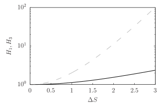
Figure 2: Plots of the functions $H_{1}$ [Eq. (36a)] (black line) and $H_{3}$ [Eq. (24)] (gray dashed line) as a function of $\Delta S$ for the channel shape given in Eq. (50).

Diagonal terms

As noted earlier, the diagonal matrix elements $\mathcal{L}_{11}\sim 1/H_{1}$ and $\mathcal{L}_{33}\sim 1/H_{3}$ depend on the shape of the channel, but not on the boundary conditions on the electrostatic potential at the channel walls. Because $H_{1}$ and $H_{3}$ increase with $\Delta S$, $\mathcal{L}_{11}$ and $\mathcal{L}_{33}$ decrease therewith. This implies that the pressure-driven volumetric fluid flow $Q$ and the chemical potential-driven excess solute flow $J_{c}^{\prime}$ diminish with increasing $\Delta S$.

Off-diagonal terms

The off-diagonal terms in Eq. (46) are controlled by the functions $\Upsilon^{\sigma,\zeta}$ and by $H_{1}$. In the following we will focus on the dependence of $\mathcal{L}_{12}$ and $\mathcal{L}_{13}$ on $\Upsilon_{1}^{\sigma,\zeta}$ and $\Upsilon_{3}^{\sigma,\zeta}$, respectively. Figure 3(a) shows for conducting channels walls that $\Upsilon_{1}^{\zeta}$ (and thus $\mathcal{L}_{12}^{\zeta}$) is almost independent of $\Delta S$, whereas $\Upsilon_{1}^{\sigma}$ (and thus $\mathcal{L}_{12}^{\sigma}$) increases more drastically as $\Upsilon_{1}^{\sigma}\propto\exp{[\Delta S]}$ at large $\Delta S$ [cf. Eq. (52c)]. Hence, counterintuitively, increasing the corrugation of the channel enhances some off-diagonal transport coefficients. Equation Eq. (46) shows that this enhancement occurs for the electric current driven by a chemical potential drop $\Delta\mu$ (with $\Delta P=\Delta V=0$) and for the excess solute flow $J_{c}^{\prime}$ driven by an external electrostatic field $\Delta V/L$ (with $\Delta P=\Delta\mu=0$).

Figure 3(b) shows that the sensitivity of $\Upsilon_{1}^{\zeta}$, and hence $\mathcal{L}_{12}$, on the boundary conditions disappears when the Debye length is much smaller than the channel section, $k_{0}\bar{h}\gg 1$, whereas it becomes significant when $k_{0}\bar{h}\lesssim 1$. In particular, Fig. 3(b) shows that in the latter regime, $\mathcal{L}_{12}^{\zeta}$ keeps the linear dependence on $k_{0}\bar{h}$ whereas $\mathcal{L}_{12}^{\sigma}$ reaches a plateau.

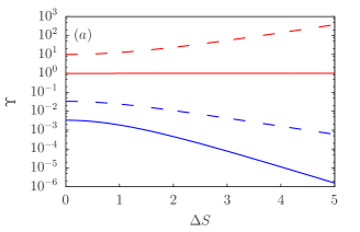
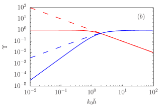
Figure 3: Plots of the functions $\Upsilon^{\zeta}_{1}$ (solid red), $\Upsilon^{\zeta}_{3}$ (solid blue), $\Upsilon^{\sigma}_{1}$ (dashed red), and $\Upsilon^{\sigma}_{3}$ (dashed blue) as a function of $\Delta S$ (panel a) and $k_{0}\bar{h}$ (panel b) for the channel shape given in Eq. (50).

The dependence of $\mathcal{L}_{13}$, on the top of its $H_{1}$-dependence, on both $\Delta S$ and $k_{0}\bar{h}$ is encoded in $\Upsilon^{\sigma,\zeta}_{3}$. Similar to $\mathcal{L}_{12}$, also $\mathcal{L}_{13}$ shows an explicit dependence on the boundary conditions. In particular, Fig. 3(a) shows that both $\mathcal{L}_{13}^{\sigma,\zeta}$ decrease with increasing $\Delta S$ and for large values of $\Delta S$ we have $\mathcal{L}_{13}^{\sigma}\propto\exp[-2\Delta S]$ and $\mathcal{L}_{13}^{\zeta}\propto\exp[-\Delta S]$. This means that the electric current induced by a pressure drop $\Delta P$ and the electroosmotic flow induced by $\Delta V$ decay exponentially with $\Delta S$. The dependence of $\mathcal{L}^{\sigma,\zeta}_{13}$ on $k_{0}\bar{h}$ is shown in Fig. 3(b). Interestingly, for large values of $k_{0}\bar{h}$ both $\mathcal{L}^{\sigma}_{13}$ and $\mathcal{L}^{\zeta}_{13}$ reach a plateau whereas for smaller values of $k_{0}\bar{h}$ they grow monotonically with $\mathcal{L}^{\sigma}_{13}\propto(k_{0}\bar{h})^{2}$ and $\mathcal{L}^{\zeta}_{13}\propto k_{0}\bar{h}$.

To understand the influence of the channel walls (i.e., conducting or dielectric) on the $\Upsilon$ functions, it is insightful to look at their relative differences through the combination

$$\Delta\Upsilon_{1,3}=2\,\dfrac{\Upsilon^{\sigma}_{1,3}-\Upsilon^{\zeta}_{1,3}}{\Upsilon^{\sigma}_{1,3}+\Upsilon^{\zeta}_{1,3}}\,.$$ (53)

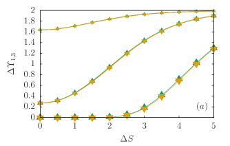
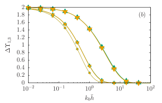
Figure 4: Plots of the functions $\Delta\Upsilon_{1}$ (downward triangles) and $\Delta\Upsilon_{3}$ (upward triangles), as a function of $\Delta S$ (panel a) and $k_{0}\bar{h}$ (panel b) for the channel shape given in Eq. (50). In (a) we use $k_{0}\bar{h}=0.1,1,10$: larger points stand for larger values of $k_{0}\bar{h}$. In (b) we use $\Delta S=0,1,3$: larger points stand for larger values of $\Delta S$.

Figure 4 shows that the functions $\Upsilon_{1,3}$ have a surprisingly similar sensitivity to the boundary conditions: whenever $\Upsilon_{1}$ changes by switching from conducting to dielectric walls, so does $\Upsilon_{3}$, and, remarkably, by almost the same amount. This means that there is no regime in which some of the Onsager coefficients are more sensitive than others upon changing the electrostatic properties of the walls. Finally, we notice from Fig. 4 that $\Delta\Upsilon_{1,3}>0$, which means [cf. Eq. (53)] that the Onsager coefficients for dielectric walls are always larger than their counterparts for conducting walls.

V.2 Single external force

So far we have discussed the general properties of the Onsager matrix and their relation to some relevant cases. In the following we discuss in detail several transport phenomena. In order to emphasize the role of the geometry and the onset of the entropic electrokinetic regime Malgaretti et al. (2014, 2015, 2016); Chinappi and Malgaretti (2018) we normalize quantities by their corresponding values in a plane channel geometry with equal average section.

V.2.1 Electrostatic driven flows

In the case that $\Delta P=\Delta\bar{\mu}=0$ a potential difference $\Delta V\neq 0$ drives an ionic current, salt flow, and electroosmotic fluid flow. In particular, the electroosmotic flow (per unit length in the $z$-direction) reads:

$$Q_{\textrm{eo}}=\mathcal{L}_{13}\frac{ze\Delta V}{L}=\frac{2\Phi\epsilon\bar{h}}{\eta}\frac{\Delta V}{L}\times\frac{\Upsilon_{3}}{H_{1}}\,.$$ (54)

This amounts to

$$Q_{\textrm{eo}}^{\zeta} =\frac{2\zeta\epsilon\bar{h}}{\eta}\frac{\Delta V}{L}\times\frac{\Upsilon^{\zeta}_{3}}{H_{1}}\,,$$ (55a)

$$Q_{\textrm{eo}}^{\sigma} =\frac{2e\sigma\bar{h}^{2}}{\eta}\frac{\Delta V}{L}\times\frac{\Upsilon^{\sigma}_{3}}{k_{0}\bar{h}H_{1}}\,.$$ (55b)

We note that Eq. (55b) coincides with Eq. (40) of Ref. Yoshida et al. (2016) and that the combination $\zeta\epsilon/\eta$ is known as the “electroosmotic mobility” Bruus (2008). For the channel as specified in Eq. (50), we show Eq. (55) as a function of $\Delta S$ in Fig. 5(a) and as a function of $k_{0}\bar{h}$ in Fig. 5(b).

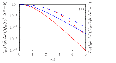
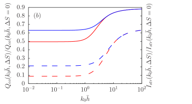
Figure 5: Electroosmotic flow $Q_{\rm eo}$ [Eq. (55)] and streaming current $I_{\rm str}$ [Eq. (58)] for conducting (red lines) and dielectric (blue lines) channel walls. Panel (a) shows $\Delta S$-dependence at $k_{0}\bar{h}=1$ (solid) and $k_{0}\bar{h}=10$ (dashed), respectively. Panel (b) shows $\Delta V$-dependence at $\Delta S=1$ (solid) and $\Delta S=1$ (dashed), respectively.

From this figure we see that both $Q_{\textrm{eo}}^{\zeta}$ and $Q_{\textrm{eo}}^{\sigma}$ vanish for highly corrugated channels (when $\Delta S\gg 0$). Meanwhile, both $Q_{\textrm{eo}}^{\zeta}$ and $Q_{\textrm{eo}}^{\sigma}$ diminish upon decreasing $k\bar{h}$. Interestingly the transition between the two plateaus occurs for $k_{0}\bar{h}\in[1:10]$, the entropic electrokinetic regime Malgaretti et al. (2014, 2015, 2016); Chinappi and Malgaretti (2018). For a straight channel, the integrals in $\Upsilon$ [Eq. (48)] become trivial and Eq. (55) simplifies to

$$Q_{\textrm{eo}}^{\zeta} =\frac{2\zeta\epsilon\bar{h}}{\eta}\frac{\Delta V}{L}\times\left[1-\mathscr{G}(k_{0}\bar{h})\right]\,,$$ (56a)

$$Q_{\textrm{eo}}^{\sigma} =\frac{2e\sigma\bar{h}^{2}}{\eta}\frac{\Delta V}{L}\times\frac{\mathscr{L}(k_{0}\bar{h})}{k_{0}\bar{h}}\,.$$ (56b)

We note that Eq. (56a) is in agreement with Eq. (50) of Ref. Delgado et al. (2007). Moreover, for a flat channel, $\psi^{\zeta}(x,y)=\psi^{\sigma}(x,y)$ provided that the surface potentials are the same: $\psi^{\zeta}(x,h)=\psi^{\sigma}(x,h)\Rightarrow\zeta=e\sigma\coth[k_{0}h]/(\epsilon k_{0})$. Inserting this into Eq. (56a) we confirm Eq. (56b).

V.2.2 Pressure driven flows

In the case that $\Delta V=\Delta\bar{\mu}=0$, a pressure difference $\Delta P\neq 0$ drives a streaming current (per unit length in the $z$-direction):

$$I_{\rm str} =\mathcal{L}_{13}ze\frac{\Delta P}{L}=\frac{2\Phi\epsilon\bar{h}}{\eta}\frac{\Delta P}{L}\times\frac{\Upsilon_{3}}{H_{1}}\,,$$ (57)

which amounts to

$$I^{\zeta}_{\rm str} =\frac{2\zeta\epsilon\bar{h}}{\eta}\frac{\Delta P}{L}\times\frac{\Upsilon^{\zeta}_{3}}{H_{1}}$$ (58a)

$$I^{\sigma}_{\rm str} =\frac{2e\sigma\bar{h}^{2}}{\eta}\frac{\Delta P}{L}\times\frac{\Upsilon^{\sigma}_{3}}{k_{0}\bar{h}H_{1}}\,.$$ (58b)

Clearly, $I_{\rm str}$ is governed by the same matrix element $\mathcal{L}_{13}$ as the electroosmotic flow (its reciprocal phenomenon) discussed above. As a consequence, $Q^{\sigma}$ and $I_{\rm str}^{\sigma}$ share the same term $\Upsilon^{\sigma}_{3}/(k_{0}\bar{h}H_{1})$ and, hence, display the same $\Delta S$ and $k_{0}\bar{h}$ dependence (see Fig. 5).

From Eq. (57) is easy to determine the streaming current between two parallel plates and to check that this agrees with Eq. (37) of Ref. Delgado et al. (2007).

V.2.3 Chemical potential steps $\Delta\bar{\mu}$

Finally, we consider the case in which flows are driven solely by a chemical potential drop $\Delta\bar{\mu}$. Accordingly, the electric current reads:

$$J_{q}=-2\gamma_{0}\bar{h}\frac{\mu_{\text{ion}}}{ze}\Phi\Delta\bar{\mu}\times\frac{\Upsilon_{1}}{H_{1}}\,.$$ (59)

which amounts to:

$$J^{\zeta}_{q} =-2\gamma_{0}\bar{h}\beta\mu_{\text{ion}}\zeta\Delta\bar{\mu}\times\frac{\Upsilon^{\zeta}_{1}}{H_{1}}\,,$$ (60a)

$$J^{\sigma}_{q} =-2\gamma_{0}\bar{h}^{2}\beta\mu_{\text{ion}}\frac{e\sigma}{\epsilon}\Delta\bar{\mu}\times\frac{\Upsilon^{\sigma}_{1}}{k_{0}\bar{h}H_{1}}\,.$$ (60b)

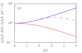
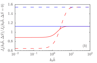
Figure 6: Electric current $J_{q}$ [Eqs. (60)] driven by a chemical potential difference, as a function of $\Delta S$ (panel a) and $k_{0}\bar{h}$ (panel b) for conducting (red lines) and dielectric (blue lines) channel walls. Panel (a) shows $\Delta S$-dependence at $k_{0}\bar{h}=1$ (solid) and $k_{0}\bar{h}=10$ (dashed), respectively. Panel (b) shows $\Delta V$-dependence at $\Delta S=1$ (solid) and $\Delta S=1$ (dashed), respectively.

For dielectric channel walls, we find with Eq. (52c) that $J^{\sigma}_{q}(\Delta S)/J^{\sigma}_{q}(\Delta S=0)=\cosh[\Delta S/2]$; hence, this ratio grows monotonically with increasing the corrugation of the channel $\Delta S$. Conversely, for conducting channel walls, Fig. 6(a) displays that $J^{\sigma}_{q}$ has a maximum for a finite value of $\Delta S$. The ionic charge currents as discussed in this section are the relevant physical phenomenon underlying reverse electrodialysis, whereby electrical energy is generated from a salt concentration difference Peters et al. (2016).

V.3 Membrane

In the following, we characterize several cases in which the channel is in series with a membrane that selectively impedes the passage of (any combination of) solvent and ions. In this scenario we can control $Q$, and the fluxes of positive, $2J^{+}=J_{c}+J_{q}$ and negative, $2J_{-}=J_{c}-J_{q}$ ions. Due to its physcal interest, in this section we focus on the full solute flow $J_{c}=J^{\prime}_{c}+\gamma_{0}Q$ rather then on $J_{c}^{\prime}$, . The general solution to Eq. (46), under the above constraints, reads:

$$\Delta\bar{\mu} =\frac{J_{c}-\left(\mathcal{L}_{12}+\gamma_{0}\mathcal{L}_{13}\right)ze\Delta V-\gamma_{0}\mathcal{L}_{33}\Delta P}{\mathcal{L}_{22}}\,,$$ (61a)

$$ze\Delta V =\frac{\mathcal{L}_{22}J_{q}-\mathcal{L}_{12}J_{c}+\left(\mathcal{L}_{12}\gamma_{0}\mathcal{L}_{33}-\mathcal{L}_{22}\mathcal{L}_{13}\right)\Delta P}{\mathcal{L}^{2}_{22}}\,,$$ (61b)

$$Q =\frac{\mathcal{L}_{13}}{\mathcal{L}_{22}}J_{q}+\mathcal{L}_{33}\Delta P\,.$$ (61c)

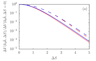
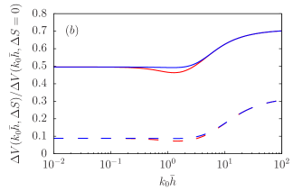
Figure 7: Electrostatic potential drop $\Delta V$ [Eq.(67b)] across a solvent permeable membrane, as a function of $\Delta S$ (panel a) and $k_{0}\bar{h}$ (panel b) for conducting (red lines) and dielectric (blue lines) channel walls. Panel (a) shows $\Delta S$-dependence at $k_{0}\bar{h}=1$ (solid) and $k_{0}\bar{h}=10$ (dashed), respectively. Panel (b) shows $\Delta V$-dependence at $\Delta S=1$ (solid) and $\Delta S=1$ (dashed), respectively.

V.3.1 Electrodes

First, we consider a membrane that allows for a net electric current, $J_{q}\neq 0$ but not for mass fluxes, $Q=J_{c}=0$. This looks like having some electrodes that close the electric circuit at zero solvent and ionic flow. When only $\Delta V$ is nonzero, Eqs. (61), at linear order in $\Phi$, gives:

$$\Delta\bar{\mu}_{V} =\frac{\mathcal{L}_{12}}{\mathcal{L}_{22}}ze\Delta V\,,$$ (62a)

$$\Delta P_{V} =\frac{\mathcal{L}_{13}}{\mathcal{L}_{33}}ze\Delta V\,,$$ (62b)

$$J_{q} =\mathcal{L}_{22}ze\Delta V\,,$$ (62c)

or, likewise,

$$\Delta\bar{\mu}_{V} =ze\Delta V\Phi\times\Upsilon_{1}\,,$$ (63a)

$$\Delta P_{V} =\frac{1}{3}\frac{\epsilon}{\beta ze}\frac{1}{\bar{h}^{2}}\Delta V\Phi\times\frac{H_{3}}{H_{1}}\Upsilon_{3}\,,$$ (63b)

$$J_{q} =-2\frac{\epsilon}{\beta ze}\bar{h}\frac{\mu_{\text{ion}}}{ze}\Delta V\times\frac{1}{H_{1}}\,.$$ (63c)

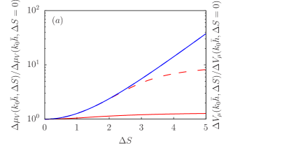
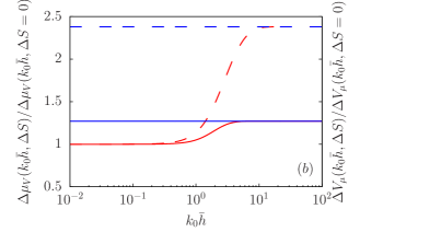
Figure 8: Chemical potential drop, $\Delta\mu$ [Eq.(63a)], as a function of $\Delta S$ (panel a) and $k_{0}\bar{h}$ (panel b) for conducting (red lines) and dielectric (blue lines) channel walls. Panel (a) shows $\Delta S$-dependence at $k_{0}\bar{h}=1$ (solid) and $k_{0}\bar{h}=10$ (dashed), respectively. Panel (b) shows $\Delta V$-dependence at $\Delta S=1$ (solid) and $\Delta S=1$ (dashed), respectively. The same quantitative behavior holds for $\Delta V$ induced by an applied chemical potential, $\Delta\mu$, when the electric current is set to zero, $Jq=0$ (see text).

Figure 8(a) shows the dependence of $\Delta\bar{\mu}_{V}$ on $\Delta S$. In particular, for both conducting and dielectric channel walls $\Delta\bar{\mu}_{V}$ increases with the corrugation of the channel $\Delta S$. In contrast, the dependence of $\Delta\bar{\mu}_{V}$ on $k_{0}\bar{h}$ is more sensitive to the conductive properties of the channel walls. While for dielectric walls $\Delta\bar{\mu}_{V}$ is independent on $k_{0}\bar{h}$, for conducting walls it reaches plateau for both $k_{0}\bar{h}\ll 1$ and $k_{0}\bar{h}\gg 1$ and it grows for $k_{0}\bar{h}\in[1:10]$ [see Fig. 8(b)]. Interestingly, the very same behavior is observed for the electrostatic potential drop, $\Delta V_{\mu}$ induced by an applied chemical potential, $\Delta\bar{\mu}$ when the electric current is set to zero, $J_{q}=0$. In this case, $\Delta V_{\mu}$ grows with $\Delta S$ for both kind of channel walls [see Fig. 8(a)]. Since both $\Delta\bar{\mu}_{V}$ and $\Delta V_{\mu}$ are proportional to $\Upsilon_{1}$, their increas upon enlaring $\Delta S$ as already shown in Fig. 6. Finally, we remark that $\Delta P_{v}$ [Eq. (63b)] is also known as the electroosmotic back/counter pressure Bruus (2008).

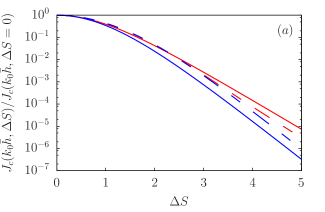
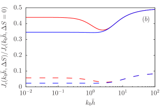
Figure 9: Solute current, $J_{c}$ [Eq.(65b)], as a function of $\Delta S$ (panel a) and $k_{0}\bar{h}$ (panel b) for conducting (red lines) and dielectric (blue lines) channel walls. Panel (a) shows $\Delta S$-dependence at $k_{0}\bar{h}=1$ (solid) and $k_{0}\bar{h}=10$ (dashed), respectively. Panel (b) shows $\Delta V$-dependence at $\Delta S=1$ (solid) and $\Delta S=1$ (dashed), respectively.

V.3.2 Open electric circuit

Second, we consider a membrane that allows for mass flows, $Q\neq 0$ and $J_{c}\neq 0$, but not for electric current, $J_{q}=0$. In this case, at linear order in $\Phi$, Eqs. (61) read:

$$\Delta\bar{\mu} =\frac{J_{c}-\left(\mathcal{L}_{12}+\gamma_{0}\mathcal{L}_{13}\right)ze\Delta V-\gamma_{0}\mathcal{L}_{33}\Delta P}{\mathcal{L}_{22}}\,,$$ (64a)

$$ze\Delta V =\frac{-\mathcal{L}_{12}J_{c}+\left(\mathcal{L}_{12}\gamma_{0}\mathcal{L}_{33}-\mathcal{L}_{22}\mathcal{L}_{13}\right)\Delta P}{\mathcal{L}^{2}_{22}}\,,$$ (64b)

$$Q =\mathcal{L}_{33}\Delta P\,.$$ (64c)

In particular, for $\Delta V=0$ this amounts to:

$$\Delta\bar{\mu} =-\frac{ze\bar{h}^{2}}{\mu_{\rm ion}\eta}\Delta P\times\frac{1}{k_{0}^{2}\bar{h}^{2}}\frac{\Upsilon_{3}}{\Upsilon_{1}}\,,$$ (65a)

$$J_{c} =-2\frac{\epsilon\bar{h}}{\beta(ze)^{2}\eta}\Delta P\times\left[\frac{1}{3}\frac{k_{0}^{2}\bar{h}^{2}}{H_{3}}-\frac{1}{H_{1}}\frac{\Upsilon_{3}}{\Upsilon_{1}}\right]\,,$$ (65b)

$$Q =-\frac{2}{3}\frac{\bar{h}^{3}}{\eta}\Delta P\times\frac{1}{H_{3}}\,.$$ (65c)

As shown in Fig. 9(a), the solute current $J_{c}$ decreases monotonically for both dielectric and conducting channel walls upon increasing the channel corrugation $\Delta S$. More surprising is the dependence of $J_{c}$ on $k_{0}\bar{h}$. Indeed, Fig. 9(b) shows that $J_{c}$ reaches a plateau for both $k_{0}\bar{h}\ll 1$ and $k_{0}\bar{h}\gg 1$ and for $k_{0}\bar{h}\simeq 1$ it displays a nonmonotonous dependence on $k_{0}\bar{h}$.

V.3.3 Solvent permeable membrane

Third, we consider a membrane that selectively permits the flow of solute, but not of ions; hence, $J_{c}=J_{q}=0$ and $J^{\prime}_{c}=\gamma_{0}Q$. Accordingly we obtain:

$$\Delta\bar{\mu} =-\frac{\gamma_{0}\mathcal{L}_{33}}{\mathcal{L}_{22}}\Delta P\,,$$ (66a)

$$ze\Delta V =\frac{\mathcal{L}_{12}\gamma_{0}\mathcal{L}_{33}-\mathcal{L}_{22}\mathcal{L}_{13}}{\mathcal{L}^{2}_{22}}\Delta P\,,$$ (66b)

$$Q =\mathcal{L}_{33}\Delta P\,,$$ (66c)

from Eq. (61). This amounts to:

$$\Delta\bar{\mu} =-\frac{1}{3}\frac{\bar{h}^{2}}{\eta}\frac{ze}{\mu_{\rm ion}}\Delta P\times\frac{H_{1}}{H_{3}}\,,$$ (67a)

$$ze\Delta V =\frac{\bar{h}^{2}}{\eta}\frac{ze}{\mu_{\rm ion}}\Phi\Delta P\times\left[\frac{1}{3}\frac{H_{1}}{H_{3}}\Upsilon_{1}-\frac{1}{k^{2}_{0}\bar{h}^{2}}\Upsilon_{3}\right]\,,$$ (67b)

$$Q =-\frac{2}{3}\frac{\bar{h}^{2}}{\eta}\Delta P\times\frac{1}{H_{3}}\,.$$ (67c)

Interestingly, in order to sustain a nonvanishing fluid flow, $Q\neq 0$, the system will excite all three external forces, i.e., we have $\Delta V\neq 0$, $\Delta P\neq 0$, and $\Delta\bar{\mu}\neq 0$. In particular, when $\Delta P$ is the only externally applied force, then from Eq. (67b) we can read off the induced streaming potential. Figure 7(a) shows that $\Delta V$ decays monotonically with $\Delta S$ for both conducting and dielectric channel walls whereas Fig. 7(b) shows that $\Delta V$ reaches a plateau for both $k_{0}\bar{h}\ll 1$ and $k_{0}\bar{h}\gg 1$ and that the sensitivity of $\Delta V$ on $k_{0}\bar{h}$ is maximum for $k_{0}\bar{h}\simeq 1$, i.e., in the entropic electrokinetic regime. Finally, by inverting Eq. (67a), Eqs. (67) show that a net fluid flow can be obtained by applying a chemical potential gradient $\Delta\bar{\mu}$. However, the net fluid flow is not a direct consequence of $\Delta\bar{\mu}$ (we recall that $\mathcal{L}_{23}=\mathcal{L}_{32}=0$). Rather $\Delta\bar{\mu}$ induces an osmotic pressure drop that eventually drives the flow.

V.3.4 Ion exchange membrane

Finally, we consider the channel to be in series with a membrane that selectively allows for flow of solvent and one ionic species, impeding the other species. Recalling that $J_{c}=(J^{+}+J^{-})/2$ and $J_{q}=(J^{+}-J^{-})/2$, when only positive ions are flowing ($J^{-}=0$) we have, $J_{c}=J_{q}$, whereas when only negative ions are flowing ($J^{+}=0$) we have, $J_{c}=-J_{q}$. Hence we have:

$$J_{c} =\frac{\mathcal{L}^{2}_{22}}{\pm\mathcal{L}_{22}-\mathcal{L}_{12}}ze\Delta V-\frac{\mathcal{L}_{12}\gamma_{0}\mathcal{L}_{33}-\mathcal{L}_{22}\mathcal{L}_{13}}{\pm\mathcal{L}_{22}-\mathcal{L}_{12}}\Delta P\,,$$ (68a)

$$\Delta\bar{\mu} =-\frac{\mathcal{L}_{12}+\gamma_{0}\mathcal{L}_{13}}{\mathcal{L}_{22}}ze\Delta V-\frac{\gamma_{0}\mathcal{L}_{33}}{\mathcal{L}_{22}}\Delta P+J_{c}\,,$$ (68b)

$$Q =\mathcal{L}_{13}\Delta V+\mathcal{L}_{33}\Delta P\,,$$ (68c)

where the sign in front of $\mathcal{L}_{22}$ is positive when positive ions are flowing and negative otherwise. We remark that within linear response $\mathcal{L}_{22}\geq\mathcal{L}_{12}$ de Groot and Mazur (1983). In contrast to the solvent permeable membrane, for the ion exchange membrane we can put one of the thermodynamic forces to zero. In particular, for electrostatic driven flows, $\Delta V\neq 0$ with $\Delta P=0$ Eqs. (68) read:

$$J_{c} =-2\frac{\mu_{\rm ion}\epsilon}{\beta(ze)^{2}\bar{h}}\Delta V\times\frac{k_{0}^{2}\bar{h}^{2}}{H_{1}}\frac{1}{\pm 1-\Phi\Upsilon_{1}}$$ (69a)

$$\Delta\bar{\mu} =ze\Delta V\Phi\times\left[\Upsilon_{1}+\frac{\epsilon}{\beta ze\mu_{\rm ion}\eta}\Upsilon_{3}\right]+J_{c}$$ (69b)

$$Q =-2\frac{\epsilon}{\beta ze}\Delta V\Phi\bar{h}\frac{1}{\eta}\times\frac{\Upsilon_{3}}{H_{1}}\,.$$ (69c)

Equation (69a) is remarkable for two reasons. First, as commented earlier, if it diverges when $\pm 1-\Phi\Upsilon_{1}\rightarrow 0$ it would require higher order corrections. Secondly, in Eq. (69a) the dimensionless potential, $\Phi$, plays a major role, i.e., it modulates the relative magnitude of the two terms in the denominator, and it is not simply a multiplicative constant as it is in all previous cases. In order to proceed with a numerical inspection of Eq. (69a) we fix the value of $\Phi$ such that $\pm 1-\Phi\Upsilon_{1}$ never vanishes. This allows us to fulfill the constraint $\mathcal{L}_{22}\geq\mathcal{L}_{12}$. Fixing the value of $\Phi$ is crucial for the dielectric case since, in order to keep the magnitude of the potential fixed, the surface charge density decreases with $k_{0}$.

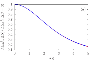
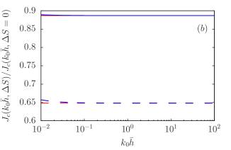
Figure 10: Solute flux $J_{c}$ [Eq.(69a)] through a semipermeable membrane as a function of $\Delta S$ (panel a) and $k_{0}\bar{h}$ (panel b) for conducting (red lines) and dielectric (blue lines) channel walls. Panel (a) shows $\Delta S$-dependence at $k_{0}\bar{h}=1$ (solid) and $k_{0}\bar{h}=10$ (dashed), respectively. Panel (b) shows $\Delta V$-dependence at $\Delta S=1$ (solid) and $\Delta S=1$ (dashed), respectively.

VI Microscopic perspective

So far we have discussed the macroscopic transport properties of the channel. However, our framework also allows us to discuss some microscopic details, such as the local electrostatic potential, $\psi_{f}(x,y)$, induced by the external forces modulated by the geometry of the channel. At first order in lubrication, the leading order force-induced correction of the Poisson equation [Eq. (1a)] reads

$$\partial^{2}_{y}\psi_{f}(x,y) =k_{0}^{2}\left[\psi_{f}(x,y)+\psi_{0}(x,y)\frac{\gamma_{f}(x)}{\gamma_{0}}\right]-\frac{ze\xi_{f}(x)}{\epsilon}\,,$$ (70)

where the right hand side follows from the perturbed ionic charge density linear in the external force, $q_{f}=\rho^{+}_{f}-\rho^{-}_{f}$. Equation (70) is solved in Appendix D for both dielectric and conducting boundary conditions. In the case of conducting walls, $\psi_{f}(x,y)$ reads

$$\psi^{\zeta}_{f}(x,y) =\frac{\psi^{\zeta}_{0}(x,y)}{2}\frac{\gamma_{f}(x)}{\gamma_{0}}$$

$$\times\left(k_{0}y\tanh[k_{0}y]-k_{0}h(x)\tanh[k_{0}h(x)]\right)$$

$$+\frac{1}{\beta ze}\frac{\xi_{f}(x)}{\gamma_{0}}\left(1-\frac{\cosh[k_{0}y]}{\cosh[k_{0}h(x)]}\right)\,,$$ (71)

while for dielectric walls we find

$$\psi^{\sigma}_{f}(x,y) =\frac{\psi^{\sigma}_{0}(x,y)}{2}\frac{\gamma_{f}(x)}{\gamma_{0}}$$

$$\times\left(k_{0}y\tanh[k_{0}y]-k_{0}h(x)\coth[k_{0}h(x)]-1\right)$$

$$+\frac{1}{\beta ze}\frac{\xi_{f}(x)}{\gamma_{0}}\,,$$ (72)

with $\psi^{\zeta}_{0}(x,y)$ and $\psi^{\sigma}_{0}(x,y)$ given by Eq. (13) and Eq. (14), respectively. We note that the contributions in Eqs. (71) and (72) are within the approximations in Eq. (25a).

VI.1 Local charge electroneutrality

At the end of Sec. III we showed that local charge neutrality is fulfilled at equilibrium in our system of interest. For the out-of-equilibrium case discussed in this section one can show that local charge neutrality holds at lowest order in the applied forces as well: Using Eq. (13) and Eq. (14) we show in Appendix E that the total ionic charge $q_{\rm tot,f}$ in a slab at $x$ precisely balances the local surface charge for both boundary conditions [$2e\sigma^{\zeta}_{f}(x)$, and $2e\sigma_{f}=0$, respectively]. Global charge neutral is then obviously satisfied at this order of approximation as well.

VI.2 Local Debye length

Using Eqs.(26),(30a) we can define a local Debye length

$$k(x)=\sqrt{\frac{\beta(ze)^{2}}{\epsilon}(\gamma_{0}+\gamma_{f}(x))}\simeq k_{0}+k_{1}(x)\,,$$ (73)

where

$$k_{1}(x) =\frac{k_{0}}{2}\frac{\gamma_{f}(x)}{\gamma_{0}}\,.$$ (74)

Interestingly, assuming a local Debye length $k(x)=k_{0}+k_{1}(x)$ and expanding Eqs. (13) and (14) for small values of $k_{1}(x)$, the terms proportional to $\gamma_{f}$ in Eqs. (71) and (72) are retrieved. Hence, our results show that the leading corrections to the local electrostatic potential proportional to the local salt concentration $\gamma_{f}(x)$ can be interpreted as being caused by a local Debye length proportional to $\gamma_{f}(x)$.

VII Conclusions

We have characterized the dynamics of a $z-z$ electrolyte embedded in a varying-section channel. We focused our analysis on channels whose section is varying smoothly enough so that we can apply a lubrication approximation to the (linearized) Poisson-Boltzmann equation —governing the electrostatic potential— as well as for the Stokes equation —governing the fluid flow. At equilibrium, we found that the Debye length stays constant up to first order in the lubrication expansion. For driven systems, we have focused on the linear response of the electrolyte to the external driving. Such a limit is relevant for weak external forces for which higher order contribution are negligibly small. Applying these approximations enabled us to derive analytical expressions for the corrections induced by the external driving to the local properties of the electrolyte. In such a regime, we have identified the set of thermodynamic forces and fluxes for which the Onsager matrix is symmetric.

Exploiting these results we have investigated several cases of experimental interest. In general, we found that increasing the channel corrugation $\Delta S$ leads to a decrease in the transport coefficients. However, our model shows that there are a few counter-examples for which the opposite holds. Indeed, the electric current induced by an ionic chemical potential imbalance $\Delta\bar{\mu}$ grows with $\Delta S$ (Fig. 6). A similar effect can be obtained when multiple thermodynamic forces are applied. For example, both the ionic chemical potential drop, $\Delta\bar{\mu}_{V}$ induced by an applied voltage $\Delta V$ when $Q=J_{c}=0$ and the electric potential drop $\Delta V_{\mu}$ induced by a chemical potential drop $\Delta\bar{\mu}$ for $J_{q}=0$ grow with the channel corrugation $\Delta S$.

Finally, we have investigated the role of the conductive properties of the channel walls on the transport coefficients. In contrast to the case of planar channel walls for which it is possible to map the solution for dielectric channel walls into that of conducting channel walls by properly rescaling the potential at the wall, when $\Delta S\neq 0$ this mapping does not hold anymore and different behavior appears. Interestingly, our results show that the difference between the transport coefficients calculated for dielectric or conducting channel walls can be significant (see Fig. 4). In particular, dielectric walls typically lead to larger transport coefficients than conducting walls. This difference is relevant only in the entropic electrokinetic regime, where the Debye length is comparable to the channel bottleneck, $k_{0}h_{\text{min}}\simeq 1$, but not to the channel widest section, $k_{0}h_{\text{max}}\simeq 1$. This clearly requires $\Delta S=\ln[h_{\text{max}}/h_{\text{min}}]\neq 0$. Indeed, as shown in Fig. 4 the difference between the transport coefficient vanishes for $k_{0}\bar{h}\rightarrow 0$, i.e., when the Debye length is too small and also for $\Delta S\rightarrow 0$, i.e., for straight channels. In particular, the difference between the transport coefficients for conducting and dielectric walls becomes not only quantitative but also qualitative in the case of the electric current driven by an ionic chemical potential drop, $\Delta\bar{\mu}$ and with $Q=J_{c}=0$. For this case the current grows monotonically with $\Delta S$ for dielectric channel walls whereas it shows a maximum for conducting channel walls.

Our results show a rich dynamics of electrolyte embedded in varying-section channels. We believe that these results can open new routes for the realization of synthetic devices aiming at energy harvesting or water desalination and can be insightful for the understanding of biological processes such as ionic transport across pores and membranes.

Appendix A Derivation of Eq. (29)

Inserting the chemical potential $\mu^{\pm}$ [Eq. (26)] into the Nernst-Planck equation (1b)], at linear order in the external force $f$ and up to quadratic in the equilibrium electrostatic potential $\psi_{0}$ (but disregarding $\mathcal{O}(f\psi_{0}^{2})$) we find

$$j_{x}^{\pm}(x,y) =v_{x}(x,y)\rho_{0}^{\pm}(x,y)-D\beta\rho_{0}^{\pm}(x,y)\partial_{x}\mu^{\pm}_{f}(x,y)$$

$$\quad+\mathcal{O}(f^{2})\,.$$ (75)

Using the local equilibrium approximation, $\partial_{y}\mu_{f}^{\pm}=0$, we find

$$J^{+} =\!\!\!\int\limits_{-h(x)}^{h(x)}\!\!\!\!\rho^{+}(x,y)v_{x}(x,y)\,\mathrm{d}y-D\beta\partial_{x}\bar{\mu}^{+}_{f}(x)\!\!\!\!\int\limits_{-h(x)}^{h(x)}\!\!\!\!\rho^{+}(x,y)\,\mathrm{d}y\,,$$ (76a)

$$J^{-} =\!\!\!\int\limits_{-h(x)}^{h(x)}\!\!\!\!\rho^{-}(x,y)v_{x}(x,y)\,\mathrm{d}y-D\beta\partial_{x}\bar{\mu}^{-}_{f}(x)\!\!\!\!\int\limits_{-h(x)}^{h(x)}\!\!\!\!\rho^{-}(x,y)\,\mathrm{d}y\,.$$ (76b)

Recalling that $\rho^{\pm}_{0}(x,y)\simeq\varrho_{0}(1\mp\psi_{0}(x,y))$, $\gamma_{0}=2\varrho_{0}$ and defining $J^{\pm}(x)=\int_{-h(x)}^{h(x)}j_{x}^{\pm}(x,y)\,\mathrm{d}y$ [Eq. (28)], $J_{c}=J^{+}+J^{-}$ and $J_{q}=J^{+}-J^{-}$, we obtain:

$$\frac{J_{c}}{D} =\beta ze\overline{\psi_{0}}(x)\partial_{x}\xi_{f}(x)-2h(x)\partial_{x}\gamma_{f}(x)+\frac{\gamma_{0}Q}{D}\,,$$ (77a)

$$\frac{J_{q}}{D} =\beta ze\overline{\psi_{0}}(x)\partial_{x}\gamma_{f}(x)-2h(x)\partial_{x}\xi_{f}(x)+\frac{\mathcal{J}_{q}(x)}{D}\,,$$ (77b)

where we identified $Q$ [cf. Eq. (20)] in the last term of Eq. (77a), and where we defined

$$\overline{\psi_{0}}(x) =\int_{-h(x)}^{h(x)}\psi_{0}(x,y)\,\mathrm{d}y\,,$$ (78)

$$\mathcal{J}_{q}(x) =\int_{-h(x)}^{h(x)}q_{0}(x,y)v_{x}(x,y)\,\mathrm{d}y\,.$$ (79)

Appendix B Derivation of Eq. (35b)

Inserting $v_{x}(x,y)$ [Eq. (19)] into $\mathcal{J}_{q}(x)$, to $\mathcal{O}(\psi_{0})$ only the pressure driven velocity $u_{P}$ remains, giving

$$\mathcal{J}_{q}(x) =\gamma_{0}\beta ze\frac{\Delta P}{2\eta L}\frac{\bar{h}^{3}}{H_{3}h^{3}(x)}$$

$$\quad\times\int_{-h(x)}^{h(x)}\left[h(x)^{2}-y^{2}\right]\psi_{0}(x,y)\,\mathrm{d}y$$ (80)

Here we used that $\partial_{x}P_{\textrm{tot},f}(x)=\Delta P\bar{h}^{3}/[H_{3}Lh^{3}(x)]+\mathcal{O}(\psi_{0})$, which follows from inserting Eq. (23) into Eq. (21). We can rewrite the integral in Eq. (80) by inserting the Poisson equation (12). Two partial integrations then give

$$\int_{-h(x)}^{h(x)}k_{0}^{2}\left[h(x)^{2}-y^{2}\right]\psi_{0}(x,y)\,\mathrm{d}y =h(x)^{2}\int_{-h(x)}^{h(x)}\partial_{y}^{2}\psi_{0}(x,y)\,\mathrm{d}y-\int_{-h(x)}^{h(x)}y^{2}\partial^{2}_{y}\psi_{0}(x,y)\,\mathrm{d}y$$

$$=\cancel{h(x)^{2}\int_{-h(x)}^{h(x)}\partial_{y}^{2}\psi_{0}(x,y)\,\mathrm{d}y}-\cancel{y^{2}\partial_{y}\psi_{0}(x,y)\bigg{|}_{-h(x)}^{h(x)}}+2\int_{-h(x)}^{h(x)}y\partial_{y}\psi_{0}(x,y)\,\mathrm{d}y$$

$$=2\int_{-h(x)}^{h(x)}[\psi_{0}(x,h(x))-\psi_{0}(x,y)]\,\mathrm{d}y\,.$$ (81)

Evaluating Eq. (34) at $x=L$, a term containing $\int_{0}^{L}\mathrm{d}x\,\mathcal{J}(x^{\prime})/h(x^{\prime})$ appears. With the above two equations and the definition of $\Upsilon_{3}$ [cf. Eq. (36d)] we find

$$\int_{0}^{L}\frac{\mathcal{J}_{q}(x)}{h(x)}\,\mathrm{d}x =\gamma_{0}\frac{\Delta P}{k_{0}^{2}\eta L}\frac{\bar{h}^{3}}{H_{3}}\beta ze\int_{0}^{L}\mathrm{d}x\int_{-h(x)}^{h(x)}\frac{\psi_{0}(x,h(x))-\psi_{0}(x,y)}{h(x)^{4}}\,\mathrm{d}y$$

$$=2\gamma_{0}\frac{\Delta P}{k_{0}^{2}\eta}\Phi\Upsilon_{3}\,,$$ (82)

which proves the appearance of $\Upsilon_{3}$ term in Eq. (35b). Note that the derivation in Eq. (B) is valid for both boundary electric conditions; hence, so is Eq. (B).

Appendix C Derivation of Eq. (38)

We recall the expression of the electroosmotic flow

$$Q_{\textrm{eo}}=\frac{\bar{h}^{3}}{H_{3}L}\int_{0}^{L}\frac{\mathrm{d}x}{h^{3}(x)}\int_{-h(x)}^{h(x)}u_{\textrm{eo}}(x,y)\,\mathrm{d}y\,,$$ (23c)

where the electroosmotic fluid velocity [Eq. (19c)] reads:

$$u_{\textrm{eo}}(x,y) =\mathcal{U}(x,y)-\mathcal{U}(x,h(x))\,,$$ (83)

with

$$\mathcal{U}(x,y) =\frac{ze}{\eta}\int\mathrm{d}y\int\mathrm{d}y\,q(x,y)\partial_{x}\psi(x,y)\,,$$ (19d)

the integrand of which, to first order in lubrication, $\psi_{0}$, and $f$, reads

$$q(x,y)\partial_{x}\psi(x,y) =q_{f}(x,y)\partial_{x}\psi_{0}(x,y)$$

$$\quad\quad+q_{0}(x,y)\partial_{x}\psi_{f}(x,y)\,.$$ (84)

By inserting Eqs.(71),(72) into Eq. (C), we find $\mathcal{O}\left(\psi_{0}f\right)$ expressions for the two terms in Eq. (C) for both boundary conditions, which we can write compactly as

$$q_{f}(x,y) \partial_{x}\psi_{0}(x,y)=\xi_{f}(x)\left[1-\theta(x,y)\right]\partial_{x}\psi_{0}(x,y)$$ (85)

$$q_{0}(x,y) \partial_{x}\psi_{f}(x,y)=-\psi_{0}(x,y)\partial_{x}\left[\xi_{f}(x)\theta(x,y)\right]\,,$$ (86)

with

$$\theta(x,y)=\begin{cases}\displaystyle 1-\frac{\cosh[k_{0}y]}{\cosh[k_{0}h(x)]}\quad\quad&\textrm{cond,}\\ \displaystyle 1&\textrm{diel,}\,.\end{cases}$$ (87)

After reshuffling $\mathcal{U}$ reads

$$\mathcal{U}_{f}(x,y) =-\frac{ze}{\eta}\int\!\mathrm{d}y\!\int\!\mathrm{d}y\Bigl{\{}\partial_{x}\left[\psi_{0}(x,y)\xi_{f}(x)(\theta(x,y)-1)\right]$$

$$\quad\quad\quad\quad\quad\quad\quad\quad\quad+\psi_{0}(x,y)\partial_{x}\xi_{f}(x)\Bigr{\}}\,.$$ (88)

We can now determine $u_{\textrm{eo}}(x,y)$ for the two different boundary conditions explicitly (note that the first term of the above integrand is zero for dielectric walls and the last term can be explicitly integrated twice),

$$u^{\zeta}_{\textrm{eo}}(x,y) =\frac{1}{\beta ze}\,\frac{\epsilon\zeta}{\eta}\,\left\{\frac{\partial_{x}\xi_{f}(x)}{\gamma_{0}}\left(1-\frac{\cosh[k_{0}y]}{\cosh[k_{0}h(x)]}\right)-\partial_{x}\left[\frac{\xi_{f}(x)}{\gamma_{0}}\frac{2k^{2}_{0}[y^{2}-h^{2}(x)]+\cosh[2k_{0}y]-\cosh[2k_{0}h(x)]}{8\cosh^{2}[k_{0}h(x)]}\right]\right\}\,,$$ (89)

$$u^{\sigma}_{\textrm{eo}}(x,y) =\frac{e\sigma}{\eta k_{0}}\frac{1}{\beta ze}\frac{\partial_{x}\xi_{f}(x)}{\gamma_{0}}\frac{\cosh[k_{0}h(x)]-\cosh[k_{0}y]}{\sinh[k_{0}h(x)]}\,.$$ (90)

Using $\mathscr{G}(x)=\tanh(x)/x$ and $\mathscr{L}(x)=\coth(x)-1/x$ as defined in Eq. (49), we obtain

$$\int_{-h(x)}^{h(x)}u^{\zeta}_{\textrm{eo}}(x,y)\,\mathrm{d}y =\frac{2h(x)}{\beta ze}\,\frac{\epsilon\zeta}{\eta}\,\frac{\partial_{x}\xi_{f}(x)}{\gamma_{0}}\left(1-\mathscr{G}[k_{0}h(x)]\right)-\frac{1}{\beta ze}\frac{\epsilon\zeta}{\eta k_{0}}\frac{\partial_{x}\left[\xi_{f}(x)\Gamma(x)\right]}{\gamma_{0}}\,,$$ (91a)

$$\int_{-h(x)}^{h(x)}u^{\sigma}_{\textrm{eo}}(x,y)\,\mathrm{d}y =2h(x)\frac{e\sigma}{\eta k_{0}}\frac{\partial_{x}\xi_{f}(x)}{\beta ze\gamma_{0}}\mathscr{L}[k_{0}h(x)]\,,$$ (91b)

with

$$\Gamma(x) =\frac{1}{4}\tanh[k_{0}h(x)]-\frac{k_{0}h(x)}{2\cosh[k_{0}h(x)]}+\frac{3k_{0}h(x)-4k_{0}^{3}h^{3}(x)}{12\cosh^{2}[k_{0}h(x)]}$$ (92)

Using Eqs. (83) and (91) we find the following expressions for $Q_{\textrm{eo}}$ [cf. Eq. (23c)]

$$Q_{\textrm{eo}}^{\zeta} =2\,\frac{\epsilon\zeta}{\eta}\,\,\frac{\bar{h}^{3}}{H_{3}L}\int_{0}^{L}\frac{1}{\beta ze}\frac{\partial_{x}\xi_{f}(x)}{\gamma_{0}}\frac{1-\mathscr{G}[k_{0}h(x)]}{h^{2}(x)}\,\mathrm{d}x-\frac{\epsilon\zeta}{\eta k_{0}}\frac{1}{\beta ze}\frac{\bar{h}^{3}}{H_{3}L}\int_{0}^{L}\frac{\partial_{x}\left[\xi_{f}(x)\Gamma(x)\right]}{\gamma_{0}}\frac{\mathrm{d}x}{h^{3}(x)}\,,$$ (93a)

$$Q_{\textrm{eo}}^{\sigma} =2\frac{e\sigma}{\eta k_{0}}\frac{\bar{h}^{3}}{H_{3}L}\int_{0}^{L}\frac{1}{\beta ze}\frac{\partial_{x}\xi_{f}(x)}{\gamma_{0}}\frac{\mathscr{L}[k_{0}h(x)]}{h^{2}(x)}\,\mathrm{d}x\,.$$ (93b)

We obtain an expression for $\partial_{x}\xi_{f}(x)$ by substituting Eq. (32) in Eq. (31). At order $\mathcal{O}((\psi_{0})^{0})$, we obtain:

$$\partial_{x}\xi_{f}(x)=-\frac{J_{q}}{2Dh(x)}+\mathcal{O}(\psi_{0})\,.$$ (94)

Inserting this expression into Eq. (93), at linear order in $\psi_{0}$, we find:

$$Q_{\textrm{eo}}^{\zeta} =-\frac{J_{q}}{D}\,\frac{\epsilon\zeta}{\eta}\,\,\frac{1}{\beta ze\gamma_{0}}\frac{\bar{h}^{3}}{H_{3}L}\int_{0}^{L}\frac{1-\mathscr{G}[k_{0}h(x)]}{h^{3}(x)}\,\mathrm{d}x-\frac{\epsilon}{\eta}\frac{\zeta}{k_{0}}\frac{1}{\beta ze}\frac{\bar{h}^{3}}{H_{3}L}\int_{0}^{L}\frac{\partial_{x}\left[\xi_{f}(x)\Gamma(x)\right]}{\gamma_{0}}\frac{\,\mathrm{d}x}{h^{3}(x)}\,,$$ (95a)

$$Q_{\textrm{eo}}^{\sigma} =-2\frac{e\sigma}{\eta k_{0}}\frac{1}{\beta ze\gamma_{0}}\frac{\bar{h}^{3}}{H_{3}L}\int_{0}^{L}\frac{J_{q}}{2Dh(x)}\frac{\mathscr{L}[k_{0}h(x)]}{h^{2}(x)}\,\mathrm{d}x\,.$$ (95b)

Comparing the above equations to Eq. (48) we see that we can write $Q_{\textrm{eo}}$ as

$$Q_{\textrm{eo}}^{\zeta} =-J_{q}\frac{\Phi\Upsilon_{3}^{\zeta}}{D\beta\eta k_{0}^{2}}-\frac{\epsilon}{\eta}\frac{\zeta}{k_{0}}\frac{1}{\beta ze}\frac{\bar{h}^{3}}{H_{3}L}\int_{0}^{L}\frac{\partial_{x}\left[\xi_{f}(x)\Gamma(x)\right]}{\gamma_{0}h^{3}(x)}\,\mathrm{d}x\,,$$ (96a)

$$Q_{\textrm{eo}}^{\sigma} =-J_{q}\frac{\Phi\Upsilon_{3}^{\sigma}}{D\beta\eta k_{0}^{2}}\,,$$ (96b)

which proves Eq. (38) up to the second term on the right hand side of Eq. (96a). Since at $\mathcal{O}\left(\zeta^{0}\right)$ we have $\xi_{f}(x)=\xi_{f}[h(x)]$, we can write

$$\int_{0}^{L}\frac{\partial_{x}F[h(x)]}{h^{3}(x)}\,\mathrm{d}x=\int_{0}^{L}\frac{\delta F[h(x)]}{\delta h(x)}\frac{\partial_{x}h(x)}{h^{3}(x)}\,\mathrm{d}x\,,$$ (97)

with $F[h(x)]=\xi_{f}(x)\Gamma(x)$, i.e., $F[h(x)]$ depends on $x$ solely through $h(x)$. Without loss of generality we can define a function $G[h(x)]$ such that

$$\frac{1}{h^{3}(x)}\frac{\delta F[h(x)]}{\delta h(x)} =\frac{\delta G[h(x)]}{\delta h(x)}$$

$$\Rightarrow\quad\int_{0}^{L}\frac{\partial_{x}F[h(x)]}{h^{3}(x)}\,\mathrm{d}x =\int_{0}^{L}\frac{\delta G[h(x)]}{\delta h(x)}\partial_{x}h(x)\,\mathrm{d}x$$

$$=G[h(L)]-G[h(0)]\,,$$ (98)

i.e., for periodic channels, $h(L)=h(0)$, we have $G(L)=G(0)$ and the last term in Eq. (96a) vanishes.

Appendix D Derivation of Eq. (71) and Eq. (72)

The solution to Eq. (70) reads

$$\psi_{f}(x,y) =-A_{0}(x)\frac{\gamma_{f}(x)}{4\gamma_{0}}\left[\cosh(k_{0}y)-2k_{0}y\sinh(k_{0}y)\right]+A_{f}(x)\cosh(k_{0}y)+\frac{1}{\beta ze}\frac{\xi_{f}(x)}{\gamma_{0}}\,,$$ (99)

where $A_{0}$ is given for conducting and dielectric walls by $A^{\zeta}_{0}=\zeta/\cosh[k_{0}h(x)]$ and $A^{\zeta}_{0}=e\sigma/(\epsilon k_{0}\sinh[k_{0}h(x)])$, respectively. The term $A_{f}(x)$ is obtained by imposing the suitable boundary conditions at the channel walls.

For conducting channel walls one has: $\psi_{f}(x,\pm h(x))=0$ and hence

$$A^{\zeta}_{f}(x)=\frac{1}{\cosh[k_{0}h(x)]}\left[\frac{\zeta}{4}\frac{\gamma_{f}(x)}{\gamma_{0}}(1-2k_{0}h(x)\tanh[k_{0}h(x)])-\frac{1}{\beta ze}\frac{\xi_{f}(x)}{\gamma_{0}}\right]\,.$$ (100)

Inserting $A^{\zeta}_{f}(x)$ into Eq. (99) we find Eq. (71) of the main text.

$$\psi^{\zeta}_{f}(x,y) =\frac{\zeta}{2}\frac{\gamma_{f}(x)}{\gamma_{0}}\left(k_{0}y\frac{\sinh[k_{0}y]}{\cosh[k_{0}h(x)]}-k_{0}h(x)\frac{\cosh[k_{0}y]\sinh[k_{0}h(x)]}{\cosh^{2}[k_{0}h(x)]}\right)+\frac{1}{\beta ze}\frac{\xi_{f}(x)}{\gamma_{0}}\left(1-\frac{\cosh[k_{0}y]}{\cosh[k_{0}h(x)]}\right)$$ (101)

$$=\frac{\psi^{\zeta}_{0}(x,y)}{2}\frac{\gamma_{f}(x)}{\gamma_{0}}\left(k_{0}y\tanh[k_{0}y]-k_{0}h(x)\tanh[k_{0}h(x)]\right)+\frac{1}{\beta ze}\frac{\xi_{f}(x)}{\gamma_{0}}\left(1-\frac{\cosh[k_{0}y]}{\cosh[k_{0}h(x)]}\right).$$ (102)

In the case of dielectric walls we fix $A^{\sigma}_{f}(x)$ by demanding $\partial_{y}\psi_{f}(x,\pm h(x))=0$. First we find

$$\psi^{\sigma}_{f}(x,y) =A^{\sigma}_{f}(x)\cosh[k_{0}y]-\frac{e\sigma}{4\epsilon k_{0}}\frac{\gamma_{f}(x)}{\gamma_{0}}\frac{\cosh[k_{0}y]-2k_{0}y\sinh[k_{0}y]}{\sinh[k_{0}h(x)]}+\frac{1}{\beta ze}\frac{\xi_{f}(x)}{\gamma_{0}}$$

$$\partial_{y}\psi^{\sigma}_{f}(x,h(x)) =A^{\sigma}_{f}(x)k_{0}\sinh[k_{0}h(x)]+\frac{e\sigma}{4\epsilon}\frac{\gamma_{f}(x)}{\gamma_{0}}\left(1+2k_{0}h(x)\coth[k_{0}h(x)]\right).$$ (103)

We now fix $A^{\sigma}_{f}(x)$ to

$$A^{\sigma}_{f}(x)=-\frac{e\sigma}{4\epsilon k_{0}}\frac{\gamma_{f}(x)}{\gamma_{0}}\frac{1+2k_{0}h(x)\coth[k_{0}h(x)]}{\sinh[k_{0}h(x)]}\,.$$ (104)

Using this results we find Eq. (72):

$$\psi^{\sigma}_{f}(x,y) =-\frac{e\sigma}{4\epsilon k_{0}}\frac{\gamma_{f}(x)}{\gamma_{0}}\left[\frac{\cosh[k_{0}y]-2k_{0}y\sinh[k_{0}y]}{\sinh[k_{0}h(x)]}+\frac{\cosh[k_{0}y]}{\sinh[k_{0}h(x)]}+\frac{2k_{0}h(x)}{\tanh[k_{0}h(x)]}\frac{\cosh[k_{0}y]}{\sinh[k_{0}h(x)]}\right]+\frac{1}{\beta ze}\frac{\xi_{f}(x)}{\gamma_{0}}$$

$$=\frac{e\sigma}{2\epsilon k_{0}}\frac{\cosh[k_{0}y]}{\sinh[k_{0}h(x)]}\frac{\gamma_{f}(x)}{\gamma_{0}}\left(k_{0}y\tanh[k_{0}y]-1-k_{0}h(x)\coth[k_{0}h(x)]\right)+\frac{1}{\beta ze}\frac{\xi_{f}(x)}{\gamma_{0}}$$

$$\psi^{\sigma}_{f}(x,y) =\frac{\psi_{0}^{\sigma}(x,y)}{2}\frac{\gamma_{f}(x)}{\gamma_{0}}\left(k_{0}y\tanh[k_{0}y]-1-k_{0}h(x)\coth[k_{0}h(x)]\right)+\frac{1}{\beta ze}\frac{\xi_{f}(x)}{\gamma_{0}}\,.$$ (105)

Appendix E Derivation of local charge neutrality at $\mathcal{O}(\psi f)$

The total ionic charge in a slab at $x$ is obtained by integrating the rhs of Eq. (70) along the transverse direction

$$ze\bar{q}=ze\overline{q_{f}}(x) =2zeh(x)\xi_{f}(x)-\beta(ze)^{2}\left[\overline{\psi_{0}}(x)\gamma_{f}(x)+\overline{\psi_{f}}(x)\gamma_{0}(x)\right]\,.$$ (106)

Here, $\overline{\psi^{\zeta}_{0}}=2\zeta\tanh[k_{0}h(x)]/k_{0}$ and $\overline{\psi^{\sigma}_{0}}=2e\sigma/(\epsilon k_{0}^{2})=2\sigma/(\beta z^{2}e\gamma_{0})$. In the conducting case,

$$\overline{\psi^{\zeta}_{f}}(x,y) =-\zeta\frac{\gamma_{f}(x)}{2\gamma_{0}}\left(2h(x)\tanh^{2}[k_{0}h(x)]-2h(x)+\frac{2\tanh[k_{0}h(x)]}{k_{0}}\right)+\frac{1}{\beta ze}\frac{\xi_{f}(x)}{\gamma_{0}}\left(2h(x)-\frac{2}{k_{0}}\tanh[k_{0}h(x)]\right)$$

$$=-\zeta h(x)\frac{\gamma_{f}(x)}{\gamma_{0}}\left(\tanh^{2}[k_{0}h(x)]-1+\frac{\tanh[k_{0}h(x)]}{k_{0}h(x)}\right)+\frac{2h(x)}{\beta ze}\frac{\xi_{f}(x)}{\gamma_{0}}\left(1-\frac{\tanh[k_{0}h(x)]}{k_{0}h(x)}\right).$$ (107)

This gives

$$\overline{q^{\zeta}_{f}}(x,y) =\cancel{2h(x)\xi_{f}(x)}-\beta ze\gamma_{f}(x)\frac{2\zeta\tanh[k_{0}h(x)]}{k_{0}}$$

$$\quad+\beta ze\zeta h(x)\gamma_{f}(x)\left(\tanh^{2}[k_{0}h(x)]-1+\frac{\tanh[k_{0}h(x)]}{k_{0}h(x)}\right)-2h(x)\xi_{f}(x)\left(\cancel{1}-\frac{\tanh[k_{0}h(x)]}{k_{0}h(x)}\right)$$ (108)

$$ze\overline{q^{\zeta}_{f}}(x,y) =\beta(ze)^{2}\zeta h(x)\gamma_{f}(x)\left(\tanh^{2}[k_{0}h(x)]-1-\frac{\tanh[k_{0}h(x)]}{k_{0}h(x)}\right)+2h(x)ze\xi_{f}(x)\frac{\tanh[k_{0}h(x)]}{k_{0}h(x)}\,.$$ (109)

Meanwhile the surface charge per surface is given by $e\sigma=-\epsilon\partial_{y}\psi_{f}(x,y=h(x))$. We find for the two surfaces

$$2e\sigma(x) =\epsilon\zeta\frac{\gamma_{f}(x)}{\gamma_{0}}\left[k_{0}^{2}h(x)\tanh^{2}[k_{0}h(x)]-k_{0}\tanh[k_{0}h(x)]-k_{0}^{2}h(x)\right]+2ze\xi_{f}(x)\frac{\tanh[k_{0}h(x)]}{k_{0}}$$

$$2e\sigma^{\zeta}(x) =\beta(ze)^{2}\zeta h(x)\gamma_{f}(x)\left[\tanh^{2}[k_{0}h(x)]-\frac{\tanh[k_{0}h(x)]}{k_{0}h(x)}-1\right]+\frac{2ze\xi_{f}(x)}{k_{0}}\tanh[k_{0}h(x)]\,.$$ (110)

Clearly, the local surface charge $2e\sigma^{\zeta}(x)$ balances the ionic charge $ze\overline{q^{\zeta}_{f}}(x,y)$ at each $x$.

In the dielectric case, there are no perturbations to the surface charge: $-\epsilon\partial_{y}\psi_{f}(x,y)=0$. Which means that local charge neutrality is satisfied only if the total perturbed ionic density vanishes $\overline{q^{\sigma}_{f}}(x,y)=0$. We find

$$\psi^{\sigma}_{f}(x,y) =-\frac{e\sigma}{2\epsilon k_{0}}\frac{\gamma_{f}(x)}{\gamma_{0}}\left(\frac{\cosh[k_{0}y]}{\sinh[k_{0}h(x)]}+k_{0}h(x)\frac{\cosh[k_{0}y]\cosh[k_{0}h(x)]}{\sinh^{2}[k_{0}h(x)]}-k_{0}y\frac{\sinh[k_{0}y]}{\sinh[k_{0}h(x)]}\right)+\frac{1}{\beta ze}\frac{\xi_{f}(x)}{\gamma_{0}}$$

$$\Rightarrow\overline{\psi^{\sigma}_{f}}(x,y) =-\frac{e\sigma}{2\epsilon k_{0}}\frac{\gamma_{f}(x)}{\gamma_{0}}\left(\frac{2}{k_{0}}+\cancel{\frac{2h(x)}{\tanh[k_{0}h(x)]}}+\frac{2}{k_{0}}-\cancel{\frac{2h(x)}{\tanh[k_{0}h(x)]}}\right)+\frac{2h(x)}{\beta ze}\frac{\xi_{f}(x)}{\gamma_{0}}$$

$$\beta ze\gamma_{0}\overline{\psi^{\sigma}_{f}}(x,y) =-\frac{2e\sigma}{ze}\frac{\gamma_{f}(x)}{\gamma_{0}}+2h(x)\xi_{f}(x)\,.$$ (111)

With Eq. (106) we then indeed find that

$$\overline{q^{\sigma}_{f}}(x,y) =2h(x)\xi_{f}(x)-\gamma_{f}(x)\frac{2\sigma}{z\gamma_{0}}+\frac{2\sigma}{z}\frac{\gamma_{f}(x)}{\gamma_{0}}-2h(x)\xi_{f}(x)=0\,.$$ (112)

References

- Alberts et al. (2007) B. Alberts, A. Johnson, J. Lewis, M. Raff, K. Roberts, and P. Walter, Molecular Biology of the Cell (Garland Science, Oxford, 2007).
- Bocquet and Charlaix (2010) L. Bocquet and E. Charlaix, Chem. Soc. Rev. 39, 1073 (2010).
- Calero et al. (2011) C. Calero, J. Faraudo, and M. Aguilella-Arzo, Phys. Rev. E 83, 021908 (2011).
- Peyser et al. (2014) A. Peyser, D. Gillespie, R. Roth, and W. Nonner, Biophysical Journal 107, 1841 (2014).
- Melnikov et al. (2017) D. V. Melnikov, Z. K. Hulings, and M. E. Gracheva, Physical Review E 95, 063105 (2017).
- Bacchin (2018) P. Bacchin, Membranes 8 (2018).
- Wheeler and Stroock (2008) T. Wheeler and A. Stroock, Nature 455, 208 (2008).
- Nipper and Dixon (2011) M. Nipper and J. Dixon, Cardiovasc. Eng. Technol. 2, 296 (2011).
- Wiig and Swartz (2012) H. Wiig and M. Swartz, Physiol. Rev. p. 1005 (2012).
- Siria et al. (2013) A. Siria, P. Poncharal, A.-L. Biance, R. Fulcrand, X. Blase, S. T. Purcell, and L. Bocquet, Nature 494, 455 (2013).
- Secchi et al. (2016) E. Secchi, S. Marbach, A. Niguès, D. Stein, A. Siria, and L. Bocquet, Nature 537, 210 (2016).
- Bonthuis et al. (2008) D. J. Bonthuis, C. Meyer, D. Stein, and C. Dekker, Physical review letters 101, 108303 (2008).
- Dubov et al. (2017) A. L. Dubov, T. Y. Molotilin, and O. I. Vinogradova, Soft Matter pp. – (2017).
- Saleh and Sohn (2003) O. A. Saleh and L. L. Sohn, Proc. Natl. Acad. Sci. U. S. A. 100, 820 (2003).
- Ito et al. (2004) T. Ito, L. Sun, M. A. Bevan, and R. M. Crooks, 20, 6940 (2004).
- Heins et al. (2005) E. A. Heins, Z. S. Siwy, L. A. Baker, and R. C. Martin, Nano Lett. 5, 1824 (2005).
- Arjmandi et al. (2012) N. Arjmandi, W. Van Roy, L. L., and G. Borghs, Anal. Chem. 84, 8490 (2012).
- Šamaj and Trizac (2016) L. Šamaj and E. Trizac, Phys. Rev. E 93, 012601 (2016).
- Reindl et al. (2017a) A. Reindl, M. Bier, and S. Dietrich, The Journal of Chemical Physics 146, 154703 (2017a).
- Reindl et al. (2017b) A. Reindl, M. Bier, and S. Dietrich, The Journal of Chemical Physics 146, 154704 (2017b).
- Brogioli (2009) D. Brogioli, Phys. Rev. Lett. 103, 058501 (2009).
- Yeh et al. (2015) H.-C. Yeh, C.-C. Chang, and R.-J. Yang, Phys. Rev. E 91, 062302 (2015).
- Siwy et al. (2005) Z. Siwy, I. D. Kosińska, A. Fuliński, and C. R. Martin, Phys. Rev. Lett. 94, 048102 (2005).
- Kosinska et al. (2008) I. Kosinska, I. Goychuk, M. Kostur, G. Schmidt, and P. Hänggi, Phys. Rev. E 77, 031131 (2008).
- Gomez et al. (2015) V. Gomez, P. Ramirez, J. Cervera, S. Nasir, M. Ali, W. Ensinger, and S. Mafe, Scientific Reports 5, 9501 EP (2015), article.
- Laohakunakorn and Keyser (2015) N. Laohakunakorn and U. F. Keyser, Nanotechnology 26, 275202 (2015).
- Lairez et al. (2016) D. Lairez, M.-C. Clochard, and J.-E. Wegrowe, Sci. Rep. 6, 38966 (2016).
- Park et al. (2006) S. Y. Park, C. J. Russo, D. Branton, and H. A. Stone, Journal of Colloid and Interface Science 297, 832 (2006).
- Mani et al. (2009) A. Mani, T. A. Zangle, and J. G. Santiago, Langmuir 25, 3898 (2009).
- Malgaretti et al. (2014) P. Malgaretti, I. Pagonabarraga, and J. M. Rubi, Phys. Rev. Lett 113, 128301 (2014).
- Chinappi and Malgaretti (2018) M. Chinappi and P. Malgaretti, Soft Matter 14, 9083 (2018).
- Malgaretti et al. (2015) P. Malgaretti, I. Pagonabarraga, and J. M. Rubi, Macromol. Symposia 357, 178 (2015).
- Malgaretti et al. (2016) P. Malgaretti, I. Pagonabarraga, and J. Miguel Rubi, The Journal of Chemical Physics 144, 034901 (2016).
- Janssen et al. (2017) M. Janssen, E. Griffioen, P. M. Biesheuvel, R. van Roij, and B. Erné, Phys. Rev. Lett. 119, 166002 (2017).
- Werkhoven et al. (2018) B. L. Werkhoven, J. C. Everts, S. Samin, and R. van Roij, Phys. Rev. Lett. 120, 264502 (2018).
- Russel et al. (1989) W. B. Russel, W. B. Saville, and W. R. Schowalter, Colloidal Dispersions (Cambridge University Press, 1989).
- Luo et al. (2015) Z.-X. Luo, Y.-Z. Xing, Y.-C. Ling, A. Kleinhammes, and Y. Wu, Nature communications 6, 6358 (2015).
- Colla et al. (2016) T. Colla, M. Girotto, A. P. dos Santos, and Y. Levin, The Journal of chemical physics 145, 094704 (2016).
- van der Heyden et al. (2005) F. H. J. van der Heyden, D. Stein, and C. Dekker, Phys. Rev. Lett. 95, 116104 (2005).
- Gross and Osterle (1968) R. J. Gross and J. Osterle, The Journal of chemical physics 49, 228 (1968).
- Ajdari (2001) A. Ajdari, Physical Review E 65, 016301 (2001).
- Ghosal (2002) S. Ghosal, Journal of Fluid Mechanics 459, 103 (2002).
- Bruus (2008) H. Bruus, Theoretical microfluidics, vol. 18 (Oxford university press Oxford, 2008).
- Yoshida et al. (2016) H. Yoshida, T. Kinjo, and H. Washizu, Computers & Fluids 124, 237 (2016).
- Delgado et al. (2007) Á. V. Delgado, F. González-Caballero, R. Hunter, L. Koopal, and J. Lyklema, Journal of colloid and interface science 309, 194 (2007).
- Peters et al. (2016) P. B. Peters, R. van Roij, M. Z. Bazant, and P. M. Biesheuvel, Phys. Rev. E 93, 053108 (2016).
- de Groot and Mazur (1983) S. R. de Groot and P. Mazur, Non-Equilibrium Thermodynamics (Dover, Amsterdam, 1983).