On the Fairness of Time-Critical Influence Maximization in Social Networks
Abstract
Influence maximization has found applications in a wide range of real-world problems, for instance, viral marketing of products in an online social network, and propagation of valuable information such as job vacancy advertisements. While existing algorithmic techniques usually aim at maximizing the total number of people influenced, the population often comprises several socially salient groups, e.g., based on gender or race. As a result, these techniques could lead to disparity across different groups in receiving important information. Furthermore, in many applications, the spread of influence is time-critical, i.e., it is only beneficial to be influenced before a deadline. As we show in this paper, such time-criticality of information could further exacerbate the disparity of influence across groups. This disparity could have far-reaching consequences, impacting people’s prosperity and putting minority groups at a big disadvantage. In this work, we propose a notion of group fairness in time-critical influence maximization. We introduce surrogate objective functions to solve the influence maximization problem under fairness considerations. By exploiting the submodularity structure of our objectives, we provide computationally efficient algorithms with guarantees that are effective in enforcing fairness during the propagation process. Extensive experiments on synthetic and real-world datasets demonstrate the efficacy of our proposal.
Index Terms:
Influence Maximization; Algorithmic Fairness; Social Networks1 Introduction
The problem of Influence Maximization has been widely studied due to its application in multiple domains such as viral marketing [1], social recommendations [2], propagation of information related to jobs, financial opportunities or public health programs [3, 4]. Over the years, extensive research efforts have focused on the cascading behavior, diffusion and spreading of ideas, or containment of diseases [5, 6, 1, 7, 8]. The idea is to identify a set of initial sources (i.e., seed nodes) in a social network who can influence other people (e.g., by propagating key information), and traditionally the goal has been to maximize the total number of people influenced in the process (e.g., who received the information being propagated) [6, 9, 10].
Real-world social networks, however, are often not homogeneous and comprise different groups of people. Due to the disparity in their population sizes, potentially high propensity towards creating within-group links [11], and differences in dynamics of influences among different groups [12], the structure of the social network can cause disparities in the influence maximization process. For example, selecting most of the seed nodes from the majority group might maximize the total number of influenced nodes, but very few members of the minority group may get influenced. In many application scenarios such as propagation of job or health-related information, such disparity can end up impacting people’s livelihood and some groups may become impoverished in the process.
Moreover, some applications are also time-critical in nature [13]. For example, many job applications typically have a deadline by which one needs to apply; if information related to the application reaches someone after the deadline, it is not useful. Similarly, in viral marketing, many companies offer discount deals only for few days (hours); getting this information late does not serve the recipient(s). More worryingly, if one group of people gets influenced (i.e., they get the information) faster than other groups, it could end up exacerbating the inequality in information access. This is possible if the majority group is better connected and more central in the network than the minority group. Thus, in time-critical application scenarios, focusing on the traditional criteria of maximizing the number of influenced nodes can have a disparate impact on different groups. This disparity in time-critical applications, in turn, can put minority and under-represented groups at a big disadvantage with far-reaching consequences. In this paper, we attempt to mitigate such unfairness in time-critical influence maximization (TCIM), and we focus on two settings: (i) where the budget (i.e., the number of seeds) is fixed and the goal is to find a seed set which maximizes the time-critical influence, we call this as TCIM-Budget problem, and (ii) where a certain quota or fraction of the population should be influenced under the prescribed time deadline, and the goal is to find such a seed set of minimal size, we call this as TCIM-Cover problem.
1.1 Our Contributions
Our first contribution is to formally introduce the notion of fairness in time-critical influence maximization, which requires that within a prescribed time deadline, the fraction of influenced nodes should be equal across different groups. We highlight, via experiments and an illustrative example, that the standard algorithmic techniques for solving TCIM-Budget and TCIM-Cover problems lead to unfair solutions, and the disparity across groups could get worse with tighter time deadline. Secondly, we study the effect of disparity of influence between groups: (i) by varying graph properties, such as connectivity and relative group sizes etc., and (ii) by varying TCIM algorithmic properties, such as seed budget, reach quota and time deadline etc.
We introduce two formulations of TCIM problems under fairness considerations, namely FairTCIM-Budget and FairTCIM-Cover. As our third contribution, we propose monotone submodular surrogates for solving both of these NP-Hard problems. Though the surrogate problems are still NP-Hard, we propose a greedy approximation with provable guarantees.
We evaluate our proposed solutions over several synthetic and two real-world social networks and show that they are successful in enforcing the aforementioned fairness notion. Enforcing fairness does come at the cost of a reduction in performance. However, as guaranteed by our theoretical results, our experiments indeed demonstrate that this cost of fairness, i.e., reduction in performance, is bounded for our approach.
2 Related Work
In this section, we briefly review the related literature on influence maximization and algorithmic fairness.
Influence Maximization. Richardson et al. [1] first introduced Influence Maximization as an algorithmic problem, and proposed a heuristic approach to find a set of nodes whose initial adoption of a certain idea/product can maximize the number of further adopters. Over the years, extensive research efforts have focused on the cascading behavior, diffusion and spreading of ideas or containment of diseases, by identifying the set of influential nodes that maximizes the influence through a network (often in real-time) [5, 6, 1, 7, 8].
Typically, identifying the most influential nodes is studied in two ways: (i) using network structural properties to find the set of most central nodes [14, 6], and (ii) formulating the problem as discrete optimization [9, 6, 15]. Kempe et al. [6], studied influence maximization under different social contagion models and showed that submodularity of the influence function can be used to obtain provable approximation guarantees. Since then, there has been a large body of work studying various extensions [9, 16, 17, 10, 18]. However, the notion of fairness in the influence maximization problem has not been studied by this line of previous works.
Fairness in Algorithmic Decision Making. Recently a growing amount of work has focused on bias and unfairness in algorithmic decision-making systems [19, 20, 21]. The aim here is to examine and mitigate unfair decisions that may lead to discrimination. Although fairness along different dimensions of political science, moral philosophy, economics, and law has been extensively studied [22, 23, 24, 25] , only a few contemporary works have investigated fairness in influence maximization, as described next.
Contemporary Works. Very recently, Fish et al. [26], proposed a notion of individual fairness in information access, but did not consider the group fairness aspects. In addition, some prior works have proposed constrained optimization problems to encourage diversity in selecting the most influential nodes [27, 28, 29, 30].
A recent paper by Rahmattalabi et al. [31], proposes group fairness in influence maximization for robust covering problems. This method is different from ours in the following ways: i) their notion of fairness is maximizing the minimum influence for any group, while we propose parity of influence among different groups; ii) they consider a setting where seeds could be deactivated randomly while we do not have any stochasticity in seed activation; iii) they consider seed nodes to spread influence only to their immediate neighbors, while we vary the allowed time deadline and show its effect on disparity among different groups. We also demonstrate the effectiveness of our methods for different time deadlines on several datasets; iv) they propose an integer linear programming set up while we propose submodular proxies, akin to the traditional methods, which can be approximately solved using the greedy heuristic.
In concurrent works, Khajehnejad et al., [32], and Tsang et al., [33], proposed methods to achieve group fairness in influence maximization. However, their works are very different from our approach in three ways: i) they propose a different problem formulation with objective that does not have submodular structural properties, ii) they only study the problem under budget constraint, and iii) they do not consider the time-critical aspect of influence in their definition of fairness for influence maximization. This could result in majority groups being influenced before the minority, and can lead to disparity in applications where the timing of being influenced/informed is critical. In our work, we introduce a submodular objective that directly addresses the time-criticality in influence maximization problem under budget constraint as well as coverage constraint.
[table]Motivating Example
3 Background on Time-Critical Influence Maximization (TCIM)
In this section, we provide the necessary background on the problem of time-critical influence maximization (henceforth, referred to as TCIM for brevity). First, we formally introduce a well-studied influence propagation model and specify the notion of time-critical influence that we consider in this paper. Then, we discuss two discrete optimization formulations to tackle the TCIM problem.
3.1 Influence Propagation in Social Network
Consider a directed graph , where is the set of nodes and is the set of directed edges connecting these nodes. For instance, in a social network the nodes could represent people and edges could represent friendship links between people. An undirected link between two nodes can be represented by simply considering two directed edges between these nodes.
There are two classical influence propagation models that are studied in the literature [6]: (i) Independent Cascade model (IC) and (ii) Linear Threshold (LT) model. In this paper, we will consider IC model and our results can easily be extended to the LT model.
In the IC model, there is a probability of influence associated with each edge denoted as . Given an initial seed set , the influence propagation proceeds in discrete time steps as follows. At , the initial seed set is “activated” (i.e., influenced). Then, at any time step , a node which was activated at time gets a chance to influence its neighbors (i.e., set of nodes ). The influence propagation process stops at time if no new nodes get influenced at this time. Under the IC model, once a node is activated it stays active throughout the process and each node has only one chance to influence its neighbors.
Note that the influence propagation under IC model is a stochastic process: the stochasticity here arises because of the random outcomes of a node influencing its neighbor based on the Bernoulli distribution . An outcome of the influence propagation process can be denoted via a set of timestamps where represents the time at which a node was activated. We have and for convenience of notation, we define to indicate that the node was not activated in the process.
3.2 Utility of Time-Critical Influence
As mentioned earlier, we focus on the application settings where the spread of influence is time-critical, i.e., it is more beneficial to be influenced earlier in the process. In particular, we adopt the well-studied notion of time-critical influence as proposed by [13]. Their time-critical model is captured via a deadline : If a node is activated before the deadline, it receives a utility of , otherwise it receives no utility. This simple model captures the notion of timing in many important real-world applications such as viral marketing of an online product with limited availability, information propagation of job vacancy information, etc.
Given the influence propagation model and the notion of time-critical aspect via a deadline , we quantify the utility of time-critical influence for a given seed set on a set of target nodes via the following:
| (1) |
where the expectation is w.r.t. the randomness of the outcomes of the IC model. The function is parametrized by deadline , set representing the set of nodes over which the utility is measured (by default, one can consider ), and the underlying graph along with edge activation probabilities . Given a fixed value of these parameters, the utility function is a set function defined over the seed set . Note that the constraint represents the node was activated and the constraint represents that the activation happened before the deadline .
3.3 TCIM as Discrete Optimization Problem
Next, we present two settings under which we study TCIM by casting it as a discrete optimization problem.
3.3.1 Maximization under Budget Constraint (TCIM-Budget)
In the maximization problem under budget constraint, we are given a fixed budget and the goal is to find an optimal set of seed nodes that maximize the expected utility. Formally, we state the problem as
| (P1) |
3.3.2 Minimization under Coverage Constraint (TCIM-Cover)
In the minimization problem under coverage constraint, we are given a quota representing the minimal fraction of nodes that must be activated or “covered” by the influence propagation in expectation. The goal is then to find an optimal set of seeds of minimal size that achieves the desired coverage constraint. We formally state the problem as
| (P2) |
3.4 Submodularity and Approximate Solutions
Next, we present some key properties of the utility function to get a better understanding of the above-mentioned optimization problems. In their seminal work, [6] showed that the utility function without time-critical deadline, i.e., , is a non-negative, monotone, submodular set function w.r.t. the optimization variable . Submodularity is an intuitive notion of diminishing returns and optimization of submodular set functions finds numerous applications in machine learning and social networks, such as influence maximization [6], sensing [34], information gathering [35], and active learning [36] (see [37] for a survey on submodular function optimization and its applications).
Chen et. al [13] showed that the utility function for the general time-critical setting for any also satisfies these properties. Submodularity is an intuitive notion of diminishing returns, stating that, for any sets , and any node , it holds that (omitting the parameters and for brevity):
Existing works [38, 39, 37] have shown that P1 and P2 are NP-Hard and hence finding the optimization solution is intractable. However, on a positive note, one can exploit the submodularity property of the function to design efficient approximation algorithms with provable guarantees [38, 37]. In particular, we can run the following greedy heuristic: start from an empty set, iteratively add a new node to the set that provides the maximal marginal gain in terms of utility, and stop the algorithm when the desired constraint on budget or coverage is met. This greedy algorithm provides the following guarantees for these two problems:.
- •
- •
4 Measuring Unfairness in TCIM
In this section, we highlight the disparity in utility across population resulting from the solution to the standard TCIM problem formulations, and introduce a measure of unfairness in TCIM.
4.1 Socially Salient Groups and Their Utilities
The current approaches to TCIM consider all the nodes in to be homogeneous. We capture the presence of different socially salient groups in the population by dividing individuals into disjoint groups. Here, socially salient groups could be based on some sensitive attribute such as gender or race. We denote the set of nodes in each group as , and we have . For any given seed set , we define the utilities for a group as by setting target nodes in Eq. 1.
4.2 Disparity in Utility Across Groups
In the standard formulations for TCIM problem, i.e., TCIM-Budget problem P1 and TCIM-Cover problem P2, the utility is optimized for the whole population without considering their groups. Clearly, a solution to TCIM problem can, in general, lead to high disparity in utilities of different groups.
In particular, this disparity in utility across groups arises from several factors in which two groups differ from each other. One of the factors is that the groups are of different sizes, i.e., one group is a minority. The different group sizes could, in turn, lead to selecting seed nodes from the majority group when optimizing for utility in problems P1 and P2. Another factor is related to the connectivity and centrality of nodes from different groups. The solution to the optimization problems P1 and P2 tend to favor nodes which are more central and have high-connectivity. Finally, given the above two factors, we note that the disparity in influence across groups can be further exacerbated for lower values of deadline in the time-critical influence maximization.
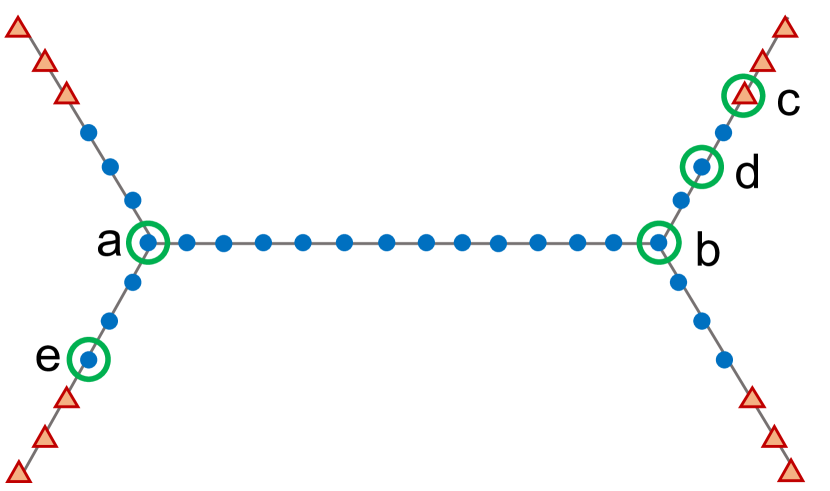
In Figure 1, we provide an example to illustrate the disparity across groups in the standard approaches to TCIM. In particular, to show this disparity, we consider the TCIM-Budget problem P1, and it is easy to extend this example to show disparity in TCIM-Cover problem P2. The graph that we consider in this example (see Figure 1 caption for details) has the two characteristic properties that we discussed above: (i) group is in minority with less than half of the size of group , (ii) group has more central nodes compared to group , and (iii) nodes in group have higher connectivity than nodes in group . We consider the probability of influence in the graph to be for all edges, and study the optimization problem P1 for budget .
For different time critical deadlines , we report the following normalized utilities: for the whole population , for the group , and for the group . Here, normalization captures the notion of “average” utility per node in a group, and automatically allows us to account for the differences in the group sizes. As can be seen in Figure 1, the optimal solution to the problem consistently picks set comprising of the most central and high-connectivity nodes. While these nodes maximize the total utility, they lead to a high disparity in the normalized utilities across groups. As the influence becomes more time-critical, i.e., is reduced, we see an increasing disparity as discussed above. For , the utility of group reduces to 0.
4.3 Measure of Unfairness
Next, in order to guide the design of fair solutions to TCIM problems, we introduce a formal notion of group unfairness in TCIM. In particular, we measure the (un-)fairness or disparity of an algorithm by the maximum disparity in normalized utilities across all pairs of socially salient groups, given by:
| (2) |
As discussed above (see Section 4.2), normalization w.r.t. group sizes captures the notion of average utility per node in a group and hence makes the measure agnostic to the group size. In the next section, we seek to design fair algorithms for TCIM problems that have low disparity (or more fairness) as measured by Eq. 2.
5 Achieving Fairness in TCIM
In this section, we seek to develop efficient algorithms for TCIM problems under fairness considerations that have low disparity measured by Eq. 2 while maintaining high performance.
5.1 Fair TCIM-Budget
5.1.1 Fairness considerations in TCIM-Budget
A fair TCIM algorithm under budget constraint should seek to achieve the following two objectives: (i) maximizing total influence for the whole population as was done in the standard TCIM-Budget problem P1, and (ii) enforcing fairness by ensuring that disparity across different groups as per Eq. 2 is low. Clearly, enforcing fairness would lead to a reduction in total influence, and we seek to design algorithms that can achieve a good trade-off between these two objectives. We formulate the following fair variant of TCIM-Budget problem P1 that captures this trade-off:
| (P3) | ||||
where is a hyperparameter which indicates the maximum level of allowed disparity among the groups. This problem might not be feasible for all the values of . So, one would have to tune this hyperparameter for feasibility and the desired level of disparity. Problem P3 has two main objectives, i.e., finding seeds which will i) maximize the total influence, which is exactly the same as the traditional influence maximization given in problem P1— here written as the sum of influences over all the groups, and, additionally, ii) minimize the disparity of influence between different groups up to the prescribed threshold.
5.1.2 Surrogate FairTCIM-Budget with guarantees
Instead of directly solving problem P3, we introduce a novel surrogate problem that would allow us to indirectly trade-off the two objectives of maximizing total influence and minimizing disparity across groups, as follows:
| (P4) |
where is a non-negative, monotone concave function.
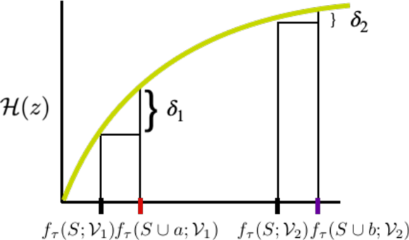
Optimizing problem P4 captures both the objectives of the original: i) maximizing influence: since the objective is monotonically increasing it encourages picking more influential nodes, ii) minimizing the disparity of influence: Passing the group influence functions through a monotone concave function rewards selecting seeds that would lead to higher influence on under-represented groups early in the selection process; this in turn helps in reducing disparity across groups under the assumption that the under-represented groups not only have lower influence in terms of total number of nodes but also have lower influnece in terms of fraction of nodes w.r.t to their groups sizes. In other words, as we are passing the group influences through a concave function, the increase in the objective would be higher when under-represented groups are influenced, as demonstrated in figure 2.
Trade-off between objectives. It is important to note that controlling the curvature of the concave function provides an indirect way to trade-off between the two objectives, i.e., i) the total influence and ii) the disparity of the solution. For instance, using has higher curvature than using and hence leads to lower disparity at the cost of lower total influence (this is demonstrated in the experimental results in Figure 4a). For our illustrative example from Section 4, we report the results for an optimal solution to FairTCIM-Budget problem P4 with . As can be seen in Figure 1, the solution leads to a drastic reduction in disparity across groups for different values of deadline compared to an optimal solution of the standard TCIM-Budget problem P1 at the cost of reduction in total influence. So, if one wants to penalize disparity of influence more one can pick function with higher curvature but at the expense of potentially lower total influence.
While it is intuitively clear that using the concave function in problem P4 reduces disparity, we also need to ensure that the solution to this problem has high influence for the whole population and that the solution can be computed efficiently. As proven in the theorem below, we can find an approximate solution to problem P4, with guarantees on the total influence, by running the greedy heuristic (as was introduced in Section 3.4).
Theorem 1
This is equivalent to the fact that the multiplicative approximation factor of the utility of FairTCIM-Budget using greedy algorithm w.r.t. the utility of an optimal solution to TCIM-Budget scales as . Note that as the curvature of the concave function increases, the approximation factor gets worse—this further highlights how the curvature of the function provides a way to trade-off the total influence and disparity of the solution. In the case of , which penalizes the disparity of the solution quite severely due to high curvature, the bound on the total influence achieved by our solution is exponentially related to the optimal solution of problem P1 which does not consider fairness. On the other hand, if , i.e., is an identity function, the problem reverts back to problem P1, whose solution might have a higher total influence but could result in high disparity, as evidenced by our experimental results in sections 6.2 and 7.2. One can pick with the appropriate curvature for the desired level of penalization of the disparity of influence at the cost of total influence. Due to lack of space, the proof of the theorem is included in the appendix.
5.2 Fair TCIM-Cover
5.2.1 Fairness considerations in TCIM-Cover
A fair TCIM algorithm under coverage constraint should seek to achieve the following two objectives: (i) minimizing the size of the seed set that achieves the desired coverage constraint as was done in the standard TCIM-Cover problem P2, and (ii) enforcing fairness by ensuring that disparity across different groups as per Eq. 2 is low. As was the case for FairTCIM-Budget problem above, enforcing fairness would lead to increasing the size of the required seed set, and we seek to design algorithms that can achieve a good trade-off between these two objectives. We formulate a fair variant of TCIM-Cover problem P2 that captures this trade-off as follows:
| (P5) | ||||
where is a hyperparameter, which determines the amount of disparity that is allowed. As in the case of problem P3, it is possible that for some values of the problem is infeasible. Problem P5 has three objectives: i) minimizing size of seed set that ii) influences a prescribed quota of the population while ii) minimizing disparity in the influence among the groups.
5.2.2 Surrogate FairTCIM-Cover with guarantees
Instead of directly solving problem P5, we introduce a novel surrogate problem that indirectly trade-offs the two objectives of minimizing the size of selected seed set and minimizing disparity, as follows:
| (P6) |
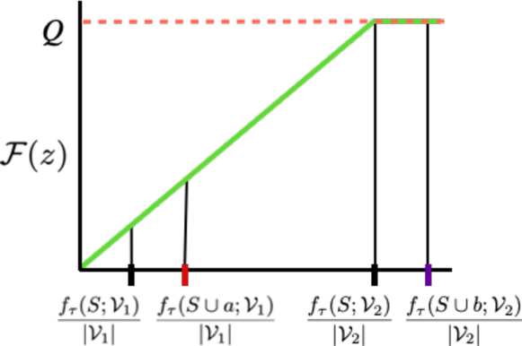
Optimizing problem P6 addresses all the objectives of problem P5 by i) minimizing the seed set size, ii) which influences all the groups up to the prescribed quota, . iii) Thereby, disparity of the feasible solution is bounded by . The key idea of using the surrogate objective function in problem P6 is the following: the problem has a constraint that enforces that at least fraction of nodes in each group are influenced by the selected seed set ; this in turn directly provides a bound on the disparity of any feasible solution to the problem as . Figure 3 provides a demonstration of the constraints we propose.
While it is intuitively clear that the solution to problem P6 reduces disparity, we also would like to bound the size of the final seed set and that the solution can be computed efficiently. As proven in the theorem below, we can find an approximate solution to problem P6, with guarantees on the final seed set size, by running the greedy heuristic (as was introduced in Section 3.4).
Theorem 2
Let us denote the output of the greedy algorithm for problem P6 by set . For group , let denote an optimal solution to the coverage problem P2 for the target nodes set to , i.e., solving problem P2 with constraint given by . Then, the size of the seed set returned by the greedy algorithm is guaranteed to have the following upper bound: .
Due to lack of space, the proof of the theorem is included in the appendix.
6 Evaluation on Synthetic Datasets
In this section, we compare the solutions of different problems on several synthetic datasets. We show that the disparity in influence is affected by varying different properties of the graphs and parameters of the algorithms.
6.1 Dataset and Experimental Setup
First we discuss how we generated the synthetic datasets and then the setup used in our experiments.
Synthetic datasets. We consider stochastic block model to generate the synthetic datasets, particularly we consider an undirected graph with nodes, where each node belongs to either group or group . The fraction of nodes belonging to each group is determined by a parameter (e.g., setting results in of the nodes to be randomly assigned to group ). Nodes are connected based on two probabilities: (i) within-group edge probability (Homophily) and (ii) across-group edge probability (Heterophily) . Placing an edge between two nodes goes as follows: given a pair of nodes , if they belong to the same group, we perform a Bernoulli trial with parameter ; otherwise we use the parameter . If the outcome of the trial is , we place an undirected edge between these two nodes. Each edge has a probability of activation, , with which the nodes can activate each other.
Experimental Setup. In our experiments we varied all the aforementioned properties of the graph. We vary each of these graph and algorithmic properties while rest of the properties are set to a default value. We experimented with several default values but as an illustration we include the results for the following default values: yielding nodes in and nodes in . We set and , which yielded total edges, out of which edges were within group , within , and edges connecting nodes across two groups. We used a constant activation probability on all edges given by . Finally, we consider the time deadline , unless explicitly stated otherwise. Evaluating utilities, as described in Eq. 1, in closed form is intractable, so we used Monte Carlo sampling to estimate these utilities. We used samples for this estimation, which yielded a stable estimation of the utility function. In all the experiments, we pick a seed set by solving the corresponding problem. Then, we use this seed set to estimate the expected number of nodes influenced in the graph using TCIM. We report the following normalized utilities: for the whole population , for the group , and for the group .
6.2 TCIM under Budget Constraints
Next, we compare the solutions of TCIM-Budget problem P1 with our solution to FairTCIM-Budget problem P4, obtained through the greedy algorithm, i.e., by iteratively picking seeds which yield maximum marginal gain. In all the figures discussed in this section, red color represents the results of TCIM-Budget problem P1, and blue color represents the results of our solution to the FairTCIM-Budget problem P4. For the experiments in this section, we used a budget of seeds.
6.2.1 Varying algorithmic properties
In this section, we vary several properties of the influence maximization algorithm and answer following questions:
— Q1: How does the choice of with different curvatures affect disparity and total influence?
— Q2: How does varying seed budget affect disparity?
— Q3: How does varying time deadline affect disparity?
— Q4: How does varying activation probabilities on the edges affect disparity?
— Q5: How effective is our method in reducing disparity?
— Q6: How much cost does our method incur?
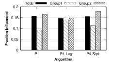
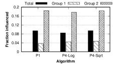
[Q1, Q5, Q6] Effect of different . Figure 4a presents the comparison of three algorithms: one solving TCIM-Budget problem P1, using the greedy heuristic; the other two solving FairTCIM-Budget problem P4, using two realizations of the concave monotone function, , given by: (i) and (ii) . Figure 4a shows the fraction of population influenced, both overall and for every group. We can observe that solving the traditional TCIM-Budget problem leads to large disparity between the fraction of nodes influenced from each group: while of nodes in group are influenced, this fraction is only for group .
On the other hand, our proposed solution to FairTCIM-Budget problem results in lower disparity
between the groups, ensuring similar fraction of influenced nodes. We can further see that , with lower curvature, performs worse than in removing the disparity, however incurring lower loss in total influence, as guaranteed by our theoretical results in Theorem 1. One could consider higher powers of the root to increase the curvature or increase the weights in problem P4 for the under-represented group. The key points are: i) with higher curvature results in lower disparity of influence at the expense of lower total influence. ii) FairTCIM-Budget problem results in lower disparity and ii) the reduction in the total influence is only marginal as guaranteed by Theorem 1. In the subsequent figures, we only show the results of for the solution to problem P4.
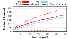
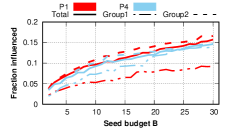
[Q2, Q5, Q6] Effect of seed budget.
Figure 4b shows the effect of different seed budgets on the number of influenced nodes (from different groups). Dotted and dash-dotted lines correspond to groups and respectively, while solid lines represent the total influence. The figure demonstrates that: (i) Disparity in the utility between both the groups increases with the increase in allowed seed budget. A reason for these differences could be the imbalances in groups sizes and average degrees, between both the groups— and comprise and of the nodes respectively. If a very big seed budget is allowed the disparity in influence might also reduce, however in many applications, due to limited resources, it is not practical to have a big budget; (ii) FairTCIM-Budget problem results in a lower disparate utility between the two groups compared to TCIM-Budget problem; (iii) this reduction in disparity is achieved at a very low cost to the total influence, as guaranteed by Theorem 1.
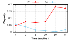
[Q3, Q5] Effect of deadline. Figure 4c compares disparity in the solutions of problems P1 and P4 as we vary the value of the deadline . Disparity is computed as the absolute difference between the fraction of individuals influenced in each group, given by Eq. 2. The figure demonstrates that: (i) disparity in group utilities does not have a unidirectional trend with increasing time deadline . One explanation for the increasing disparity— for , could be that the seed nodes or the most influential nodes are propagating influence in both the groups, but as we increase the time deadline, Group , with more nodes and edges, is more efficient at propagating influence compared to Group , so it results in a larger disparity. But, after a threshold of increase in both groups are being influenced because longer cascades are allowed. Hence the disparity lowers and then plateaus, for . One could imagine a case, as shown in the motivating example in Figure 1, where seed nodes are surrounded by nodes of only one group, in this case increasing time deadline could yield a lower disparity. (ii) Our proposed method, given by problem P4, yields solutions which result in much lower disparity.
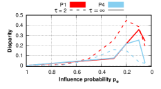
[Q4, Q5] Effect of activation probabilities. Figure 5a shows the disparity in influence for different activation probabilities . The results show that: i) lower activation probabilities could result in larger disparity. This makes intuitive sense, since with lower activation probabilities less nodes have a chance to be influenced. We are using an imbalanced graph, both in terms of group sizes and within and across group connectivity. It is very likely that the seeds selected might belong to the majority group and will have more connections to the nodes from their own group. With low activation probabilities less number of nodes are expected to be influence and the biases in the graph structure would become more pronounced, as evidenced by the results. With the high activation probabilities more number of nodes are expected to be influenced so the disparity in the influence is lower, as demonstrated by the results. ii) Lower values of tend to have a higher disparity compared to the higher values of . The intuition presented in the previous paragraph is confirmed with this experiment. iii) Our method consistently results in a lower disparity. The difference in disparities resulting from the solution of our method compared to the solution of traditional method in more pronounced for lower activation probabilities.
6.2.2 Varying graph properties
In this section, we vary several graph properties and answer following evaluation questions:
— Q1: How does varying group sizes affect the disparity?
— Q2: How does varying connectivity among the groups affect the disparity?
— Q3: How effective is our method in reducing disparity?
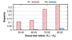
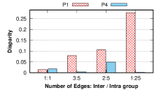
[Q1, Q3] Effect of group sizes. Figure 5b shows the effect of group sizes . x-axis represents ratio of the nodes belonging to the two groups and y-axis represents disparity. i) The figure confirms our hypothesis that imbalance in a graph could lead to disparate influence, as motivated in the illustrative example given in Figure 1. Since we are considering a of , i.e., across vs within group edge probability ratios, even slight imbalance in the group sizes could result in a high disparity. The seed nodes or influential nodes are more likely to be from the dominant group and are more likely to be connected with nodes from their own groups. ii) On the other hand our proposed method results in almost no or very little disparity of influence, as it encourages to pick seeds which influence under-represented group.
[Q2, Q3] Effect of graph connectivity.
Figure 5c demonstrates the importance of the graph structure, particularity connectivity between the two groups, characterized by
. x-axis shows the ratio of across and within group edge probabilities. i) The figure validates our hypothesis that the majority group containing more influential nodes fares better in TCIM-Budget problem, as proposed in figure 1. Groups and comprise and of the nodes, respectively. As we increase the group-preferential attachment, represented by x-axis of figure 5c, influential nodes are more likely to have connections within the group , which in turn results in disparate influence propagation. ii) However, our proposed method performs better because it gives less weight to the nodes influenced from the majority group compared to the minority. Hence, our method encourages picking seed nodes which will influence the minority group, as explained in figure 2.
Takeaways. In this section we demonstrated that: (i) solving TCIM-Budget problem can lead to disparity of influence in different groups; (ii) the amount of disparity depends on the time deadline, activation probability, relative group sizes, budget, and connectivity of the graph; and (iii) instead, solving FairTCIM-Budget results in lower disparity of influence, with marginal reduction in overall influence, as guaranteed by Theorem 1.
6.3 TCIM under Coverage Constraints
Next, we compare solutions of TCIM-Cover problem P2, and our solution to FairTCIM-Cover problem P6. We solve both the problems using the greedy algorithm, i.e., iteratively picking seeds which maximize the constraints of problems P2 and P6 until the required quota is reached. The goal is to reach the prescribed quota , with minimum number of seeds. In all the figures discussed in this section, red color represents the results of TCIM-Cover problem P2, and blue color represents the results of our solution to FairTCIM-Cover problem P6. We answer the following question in this section:
— Q1: How does our method fare compared to the traditional method over the iterations of the algorithm?
— Q2: How effective is our method in reducing disparity for different reach quotas?
— Q3: How much cost does our method incur?
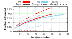
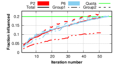
[Q1] Effect of iterations.
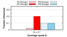
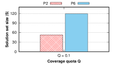
Figure 6a shows how the fraction of population influenced changes with seed selection at each iteration. Solid lines represent total influence while dash-dotted lines and dotted lines represent groups and , respectively. In this experiment, was set to which is represented by the horizontal green line. The figure demonstrates that: (i) both methods reach the required quota of the population; (ii) however, only the solution set of FairTCIM-Cover problem P6 reaches the required quota in both the groups; (iii) while maintaining roughly similar utility for both the groups throughout the iterations; (iv) and it does so at a small expense of additional seeds, as guaranteed in Theorem 2.
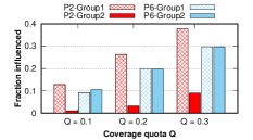
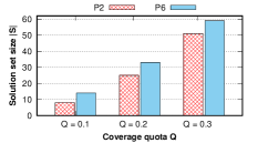
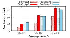
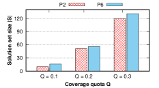
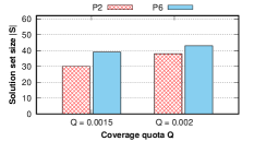
[Q2, Q3] Effect of quota Q. Figure 6b shows fractions of individuals that are influenced for different quota : (i) for different values of the required quota, traditional method given by problem P2 results in disparate utility between both the groups which is most likely due imbalance in group sizes and connectivity. (ii) Seeds selected by solving problem P6 result in a more equal utility because our method explicitly requires every group to be influence up to quota . Depending on the graph structure, our method could result in a disparity up to . The objective in the constraint given in problem P6 only increases if nodes belonging to the groups are influenced which have not reached the required quota, as demonstrated in figure 3. A higher disparity between groups could occur when it is not possible to influence the under-influenced group without influencing the already over-influenced group. In practice a higher disparity could occur, e.g, if one of the groups is very small and very sparsely connected within the group, which is unlikely to occur in practice. (iii) FairTCIM-Cover problem P6 uses only a small number of additional seeds, as guaranteed by Theorem 2.
Takeaways. We compared the result of TCIM-Cover problem P2 and our solution to FairTCIM-Cover problem P6. The results show that: (i) both methods reach the same fraction of the population; (ii) however, only FairTCIM-Cover problem results in seed sets influencing the required quota in all the groups and results in a very low disparity between groups; and (iii) lastly, FairTCIM-Cover yields only slightly larger solution sets as guaranteed by Theorem 2.
7 Experiments on Real-World Datasets
In this section, we evaluate our proposed solutions using two real-world datasets. We describe the datasets and the details of the experiments, and then present our findings.
7.1 Dataset and Experimental Setup
Next, we describe the datasets we used to evaluate our proposed methods, followed by the experimental setup.
Rice-Facebook dataset. To evaluate our proposed methods, we used Rice-Facebook dataset collected by [40], where they capture the connections between students at the Rice University. The resulting network consists of nodes and undirected edges. Each node has attributes: (i) the residential college id (a number between ), (ii) age (a number between ), and (iii) a major ID (which is in the range ).
We grouped the nodes (students) into four groups based on their age attributes. We experimented with all four groups while running our algorithms but present the results using only 2 groups which showed the highest disparity. We considered nodes with ages and as group and age as group . Group has nodes and within-group edges. Whereas, group has nodes and within-group edges. Overall, there are across-group edges going between nodes in and .
Instagram-Activities dataset. This dataset was gathered by [41]. It comprises nodes and undirected edges. The nodes represent a subset of Instagram users. There exists an edge between two nodes if either of them have liked or commented on each other’s photos. Each node has a binary-valued gender attribute, i.e., male or female. of the nodes belong to the male group. There are within-group edge among males and within-group edges among females, while there are across-group edges.
Experimental Setup. In all the experiments using Rice-Facebook dataset, we show the results for activation probability . All the other parameter were the same as described in section 6.1. For experiments using Instagram-Activities dataset we show the results with activation probability , time deadline , reach quota and seed budget . We also experimented with other values of these parameters and get similar results. For Instagram-Activities we restrict the seeds to be picked from randomly selected nodes from the graph. However the influence was evaluated and propagated on the entire network. We used sample for Facebook-Rice dataset and samples for Instagram-Activities dataset for Monte Carlo estimation of the influence of a node, which yielded very low-variance influence estimates.
7.2 TCIM under Budget Constraint
In this section, we compare the results of TCIM-Budget problem P1 and our solution to FairTCIM-Budget problem P4. Red color in all the figures discussed in this section corresponds to the solution of TCIM-Budget problem P1 and the blue color corresponds to our solution of FairTCIM-Budget problem P4. In all the experiments in this section we used a seed budget . We answer the following evaluation questions using two real-world datasets in this section:
— Q1: How does the choice of with different curvatures affect disparity?
— Q2: How does varying seed budget affect disparity?
— Q3: How does varying time deadline affect disparity?
— Q4: How effective is our method in reducing disparity?
— Q5: How much cost does our method incur?
[Q1, Q4, Q5] Effect of different .
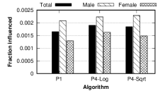
In Figures 7a and 9a, we compare the results of TCIM-Budget problem P1 and FairTCIM-Budget problem P4 using two realizations of , given by: (i) and (ii) . In Figures 7a the total influence are shown for all the groups while the group influences are shown for 2 out of the 4 groups which showed the maximum disparity. The results demonstrates that: (i) At a marginal reduction of total influence, as guaranteed by Theorem 1, our proposed method significantly reduces disparity in influence in case of Rice-Facebook dataset. However, in the Instagram-Activities dataset solving FairTCIM-Budget problem results in a higher total influence while achieving same or lower disparity for both the groups. This is in line with the finding by [42], which, using this dataset, shows that picking more diverse seeds could increase the total influence compared to greedy degree based seeding strategy. Greedy heuristic is just an approximation of the optimal solution. The optimal solution of the unfair problem cannot yield a lower influence compared to the optimal solution of the fair problem, as it adds additional constraints; (ii) as hypothesized in Section 5.1, a higher curvature function, , leads to a bigger reduction in disparity compared to . In Instagram-Activities dataset does not reduce disparity, however it does result in a higher fraction of influence in under-influenced group.
[Q2, Q4, Q5] Effect of seed budget. Figure 7b demonstrates the effect of allowed seed budget on the group and total influences. Groups and are represented by dash-dotted lines and dotted lines respectively and solid lines correspond to total influence. Similar to the results on synthetic dataset presented in section 6.2, i) the disparity between the groups seems to increase with increasing budget and ii) our method consistently results in lower disparity for different seed budgets, iii) while incurring a very small cost of total influence.
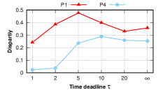
[Q3, Q4] Effect of time deadline. Figure 7c shows the effect of different time deadlines on the disparity between group influences, as calculated by Eq. 2. It demonstrates that: (i) the disparity of influence among groups
increases as the value of increase, refer to section 6.2 for an intuitive explanation and, ii) our method is very effective in reducing disparity for different values of .
Takeaways. We demonstrated that: (i) FairTCIM-Budget, our proposed method, yields more fair solutions; (ii) this fairness is achieved at a very small reduction of the total influence compared to TCIM-Budget problem, as guaranteed by Theorem 1.
7.3 TCIM under Coverage Constraint
Next, we compare TCIM-Cover problem P2 and our solution to FairTCIM-Budget problem P6. Red color in all the figures discussed in this section corresponds to the solution of TCIM-Cover problem P2 and the blue color corresponds to our solution of FairTCIM-Cover problem P6. We answer the following evaluation question using a real-world dataset.
— Q1: How does our method fare compared to the traditional method over the iterations of the algorithm?
— Q2: How effective is our method in reducing disparity for different reach quotas?
— Q3: How much cost does our method incur?
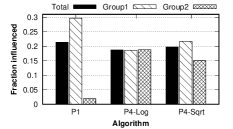
[Q1] Effect of iterations. In Figures 8a we compare iterations of problem P2 and problem P6, realized with the log function.
In each iteration, one seed is selected. Green line represents the required quota of coverage. Dashed-dotted lines, dotted lines and solid lines represent group , group and total population, respectively. Similar to the results on Synthetic dataset, i) our method consistently results in lower disparity between the two groups, which showed the highest disparity, throughout the iteration of the seed selection algorithm; ii) our method influences all the groups up to prescribed quota; iii) by using small number of additional seeds.
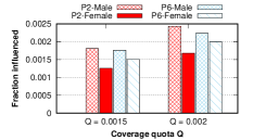
[Q2, Q3] Effect of quota. Figures 8b, 8c, 9a and 9c demonstrate similar results to the synthetic dataset described in section 6.3. The keypoint is that all the groups are covered up to the required quotas with the solution set of FairTCIM-Cover problem by using only a small number of additional seeds.
Takeaways. We compared the TCIM-Cover and FairTCIM-Cover problems in this section using a real world dataset. The results demonstrate that our method is i) effective in reducing disparity ii) by using a small additional number of seeds.
8 Conclusions
In this paper, we considered the important problem of time-critical influence maximization (TCIM) under (i) budget constraint (TCIM-Budget) and (ii) coverage constraint (TCIM-Cover). We showed that the existing algorithmic techniques aimed at maximizing total influence in the population could lead to a huge disparity in utility across the underlying groups. This can put minority groups at a big disadvantage with far-reaching consequences. To ensure that different groups are fairly treated, we proposed a notion of fairness and formulated two novel problems to solve TCIM under fairness considerations, namely, FairTCIM-Budget and FairTCIM-Cover. By introducing surrogate objective functions with submodular structural properties, we provided computationally efficient algorithms with desirable guarantees. Experiments over synthetic and real-world datasets demonstrated that our algorithms lead to low disparity in the time-critical influence propagation. This work opens up a variety of new research problems, including extensions to different notions of fairness, considering more complex models of time-criticality in information propagation (such as discounting with time), and developing new optimization methods for solving the fair TCIM problem formulations.
Acknowledgements
This research was supported in part by a European Research Council (ERC) Advanced Grant for the project “Foundations for Fair Social Computing”, funded under the European Union’s Horizon 2020 Framework Programme (grant agreement no. 789373)
Appendix A Proof of theorem 1
Proof:
Since the composition of a non-decreasing concave and a non-decreasing submodular function is submodular [43], the objective function in the following problem
| (P4) |
is monotone submodular function. Let be the optimal solution and be the output of the greedy algorithm for the problem P4, with a fixed budget . Let be an optimal solutions for the following problem
| (P1) |
Appendix B Proof of theorem 2
Proof:
The constraint in the following problem
| (P6) |
could be rewritten as follows,
The objective function in the constraint is monotone submodular function because monotone submodular functions remain monotone submodular under truncation: if is monotone submodular so is for any constant , and monotone submodular functions are closed under addition [37]. Let be the optimal solution and be the greedy solution of problem P6 for a fixed quota . Let be the optimal solution of the following problem:
| (P2) |
with target nodes set to and quota set to . Then, following the standard guarantees of the submodular optimization [37] (also see Section 3.4) we have the following bound:
| (7) |
Since is the optimal solution of problem P6, where all the groups reach the prescribed quota , must be at-least as small as any other other set which also reaches all the groups up to the quota . Hence,
| (8) |
Combining equations 7 and 8 we get
which concludes the proof. ∎
Appendix C Results Facebook-Snap Dataset
In this Section, we show the results using the Facebook-Snap dataset proposed by [44]. The dataset comprise nodes and undirected edges. We used spectral clustering to identify topological groups in the graph. The five groups comprise , , , and nodes. We run our algorithms for the entire dataset but report the results only for groups and , as these groups showed the most disparity in influence using the traditional methods of influence maximization. We used edge weight on and . Rest of the parameters were similar to the experiments described in the paper.
The results are shown in figure 10 show that our methods are effective in reducing disparity when considering topological grouping of graphs.
References
- [1] M. Richardson and P. Domingos, “Mining knowledge-sharing sites for viral marketing,” in KDD, 2002.
- [2] M. Ye, X. Liu, and W.-C. Lee, “Exploring social influence for recommendation: a generative model approach,” in SIGIR. ACM, 2012, pp. 671–680.
- [3] A. Banerjee, A. G. Chandrasekhar, E. Duflo, and M. O. Jackson, “The diffusion of microfinance,” Science, vol. 341, no. 6144, 2013.
- [4] A. Yadav, H. Chan, A. Xin Jiang, H. Xu, E. Rice, and M. Tambe, “Using social networks to aid homeless shelters: Dynamic influence maximization under uncertainty,” in AAMAS, 2016, pp. 740–748.
- [5] J. Leskovec, A. Krause, C. Guestrin, C. Faloutsos, J. VanBriesen, and N. Glance, “Cost-effective outbreak detection in networks,” in KDD. ACM, 2007, pp. 420–429.
- [6] D. Kempe, J. Kleinberg, and É. Tardos, “Maximizing the spread of influence through a social network,” in KDD, 2003.
- [7] J. Wallinga and P. Teunis, “Different epidemic curves for severe acute respiratory syndrome reveal similar impacts of control measures,” American Journal of epidemiology, vol. 160, no. 6, pp. 509–516, 2004.
- [8] M. Gomez-Rodriguez, J. Leskovec, and A. Krause, “Inferring Networks of Diffusion and Influence,” in KDD, 2010.
- [9] A. Goyal, F. Bonchi, L. V. Lakshmanan, and S. Venkatasubramanian, “On minimizing budget and time in influence propagation over social networks,” Social network analysis and mining, vol. 3, no. 2, pp. 179–192, 2013.
- [10] T. Carnes, C. Nagarajan, S. M. Wild, and A. Van Zuylen, “Maximizing influence in a competitive social network: a follower’s perspective,” in EC. ACM, 2007, pp. 351–360.
- [11] M. McPherson, L. Smith-Lovin, and J. M. Cook, “Birds of a feather: Homophily in social networks,” Annual review of sociology, vol. 27, no. 1, pp. 415–444, 2001.
- [12] A. Singla and I. Weber, “Camera brand congruence in the flickr social graph,” in WSDM, 2009, pp. 252–261.
- [13] W. Chen, W. Lu, and N. Zhang, “Time-critical influence maximization in social networks with time-delayed diffusion process,” in AAAI, 2012.
- [14] N. Kourtellis, T. Alahakoon, R. Simha, A. Iamnitchi, and R. Tripathi, “Identifying high betweenness centrality nodes in large social networks,” Social Network Analysis and Mining, vol. 3, no. 4, pp. 899–914, 2013.
- [15] M. Babaei, B. Mirzasoleiman, M. Jalili, and M. A. Safari, “Revenue maximization in social networks through discounting,” Social Network Analysis and Mining, vol. 3, no. 4, pp. 1249–1262, 2013.
- [16] S. Bharathi, D. Kempe, and M. Salek, “Competitive influence maximization in social networks,” in International workshop on web and internet economics. Springer, 2007, pp. 306–311.
- [17] C. Budak, D. Agrawal, and A. El Abbadi, “Limiting the spread of misinformation in social networks,” in WWW, 2011.
- [18] K. Huang, S. Wang, G. Bevilacqua, X. Xiao, and L. V. Lakshmanan, “Revisiting the stop-and-stare algorithms for influence maximization,” Proceedings of the VLDB Endowment, vol. 10, no. 9, pp. 913–924, 2017.
- [19] C. Dwork, M. Hardt, T. Pitassi, O. Reingold, and R. Zemel, “Fairness through awareness,” in ITCS. ACM, 2012, pp. 214–226.
- [20] M. Feldman, S. A. Friedler, J. Moeller, C. Scheidegger, and S. Venkatasubramanian, “Certifying and removing disparate impact,” in KDD. ACM, 2015, pp. 259–268.
- [21] M. Hardt, E. Price, N. Srebro et al., “Equality of opportunity in supervised learning,” in NIPS, 2016, pp. 3315–3323.
- [22] V. Conitzer, R. Freeman, N. Shah, and J. W. Vaughan, “Group fairness for the allocation of indivisible goods,” in AAAI, 2019.
- [23] B. Fain, K. Munagala, and N. Shah, “Fair allocation of indivisible public goods,” in EC. ACM, 2018, pp. 575–592.
- [24] E. Segal-Halevi and W. Suksompong, “Democratic fair allocation of indivisible goods,” in IJCAI, 2018, pp. 482–488.
- [25] W. Suksompong, “Approximate maximin shares for groups of agents,” Mathematical Social Sciences, vol. 92, pp. 40–47, 2018.
- [26] B. Fish, A. Bashardoust, danah boyd, S. A. Friedler, C. Scheidegger, and S. Venkatasubramanian, “Gaps in Information Access in Social Networks,” in WWW, 2019.
- [27] R. Bredereck, P. Faliszewski, A. Igarashi, M. Lackner, and P. Skowron, “Multiwinner elections with diversity constraints,” in AAAI, 2018.
- [28] P. Faliszewski, P. Skowron, A. Slinko, and N. Talmon, “Multiwinner voting: A new challenge for social choice theory,” Trends in computational social choice, vol. 74, 2017.
- [29] N. Benabbou, M. Chakraborty, X.-V. Ho, J. Sliwinski, and Y. Zick, “Diversity constraints in public housing allocation,” in AAMAS, 2018, pp. 973–981.
- [30] S. Aghaei, M. J. Azizi, and P. Vayanos, “Learning optimal and fair decision trees for non-discriminative decision-making,” arXiv preprint arXiv:1903.10598, 2019.
- [31] A. Rahmattalabi, P. Vayanos, A. Fulginiti, E. Rice, B. Wilder, A. Yadav, and M. Tambe, “Exploring algorithmic fairness in robust graph covering problems,” in Advances in Neural Information Processing Systems, 2019, pp. 15 750–15 761.
- [32] M. Khajehnejad, A. A. Rezaei, M. Babaei, J. Hoffmann, M. Jalili, and A. Weller, “Adversarial graph embeddings for fair influence maximization over social networks,” arXiv preprint arXiv:2005.04074, 2020.
- [33] A. Tsang, B. Wilder, E. Rice, M. Tambe, and Y. Zick, “Group-Fairness in Influence Maximization,” arXiv preprint arXiv:1903.00967, 2019.
- [34] A. Krause and C. Guestrin, “Near-optimal observation selection using submodular functions,” in AAAI, 2007, pp. 1650–1654.
- [35] A. Singla, E. Horvitz, P. Kohli, R. White, and A. Krause, “Information gathering in networks via active exploration,” in IJCAI, 2015, pp. 891–988.
- [36] A. Guillory and J. A. Bilmes, “Active semi-supervised learning using submodular functions,” in UAI, 2011, pp. 274–282.
- [37] A. Krause and D. Golovin, “Submodular function maximization.” 2014.
- [38] G. Nemhauser, L. Wolsey, and M. Fisher, “An analysis of the approximations for maximizing submodular set functions,” Math. Prog., vol. 14, pp. 265–294, 1978.
- [39] U. Feige, “A threshold of ln n for approximating set cover,” Journal of the ACM, vol. 45, pp. 314–318, 1998.
- [40] A. Mislove, B. Viswanath, K. P. Gummadi, and P. Druschel, “You are who you know: inferring user profiles in online social networks,” in WSDM. ACM, 2010, pp. 251–260.
- [41] A.-A. Stoica, C. Riederer, and A. Chaintreau, “Algorithmic glass ceiling in social networks: The effects of social recommendations on network diversity,” in Proceedings of the 2018 World Wide Web Conference, 2018, pp. 923–932.
- [42] A.-A. Stoica and A. Chaintreau, “Fairness in social influence maximization,” in Companion Proceedings of The 2019 World Wide Web Conference, 2019, pp. 569–574.
- [43] H. Lin and J. Bilmes, “A class of submodular functions for document summarization,” in Proc. ACL: HLT - Vol. 1, 2011, pp. 510–520.
- [44] J. J. McAuley and J. Leskovec, “Learning to discover social circles in ego networks.” in NIPS, vol. 2012. Citeseer, 2012, pp. 548–56.