]also at Jawaharlal Nehru Centre For Advanced Scientific Research, Jakkur, Bangalore, India

Deep-learning-assisted detection and termination of spiral- and broken-spiral waves in mathematical models for cardiac tissue

Abstract

Unbroken and broken spiral waves, in partial-differential-equation (PDE) models for cardiac tissue, are the mathematical analogs of life-threatening cardiac arrhythmias, namely, ventricular tachycardia (VT) and ventricular-fibrillation (VF). We develop a (a) deep-learning method for the detection of unbroken and broken spiral waves and (b) the elimination of such waves, e.g., by the application of low-amplitude control currents in the cardiac-tissue context. Our method is based on a convolutional neural network (CNN) that we train to distinguish between patterns with spiral waves $\mathscr{S}$ and without spiral waves $\mathscr{NS}$. We obtain these patterns by carrying out extensive direct numerical simulations (DNSs) of PDE models for cardiac tissue in which the transmembrane potential $V$, when portrayed via pseudocolor plots, displays patterns of electrical activation of types $\mathscr{S}$ and $\mathscr{NS}$. We then utilise our trained CNN to obtain, for a given pseudocolor image of $V$, a heat map that has high intensity in the regions where this image shows the cores of spiral waves. Given this heat map, we show how to apply low-amplitude Gaussian current pulses to eliminate spiral waves efficiently. Our in silico results are of direct relevance to the detection and elimination of these arrhythmias because our elimination of unbroken or broken spiral waves is the mathematical analog of low-amplitude defibrillation.

The normal pumping of blood by mammalian hearts is initiated by electrical waves of excitation that propagate through cardiac tissue and induce cardiac contractions. The abnormal propagation of such waves can lead to cardiac arrhythmias, like ventricular tachycardia (VT) and ventricular fibrillation (VF), which cause sudden cardiac death (SCD) that is among the leading causes of death in the industrialised world Mehra (2007); Majumder et al. (2011); Clayton et al. (2011) (see, e.g., Refs. Honnekeri et al. (2014); Zheng et al. (2001) for SCD data from India and the USA). The principal cause of VT and VF are spiral or scroll waves of electrical activation in cardiac tissue; unbroken (broken) spiral or scroll waves are associated with VT (VF). Such waves have been studied in vivo Berul et al. (1996); Chinushi et al. (2003); Gelzer et al. (2008) in mammalian hearts, in vitro Davidenko et al. (1990); Ikeda et al. (1996); Valderrábano et al. (2000); Lim et al. (2006) in cultures of cardiac myocytes, and in silico Shajahan et al. (2007, 2009); Nayak and Pandit (2014), in mathematical models for cardiac tissue. The efficient elimination of such spiral or scroll waves and the subsequent restoration of the normal rhythm of a mammalian heart, is a difficult problem; this can be attempted by pharmacological means Moreno et al. (2013) or by electrical means called defibrillation Sinha et al. (2001). Defibrillation by the application of low-amplitude current pulses is the grand-challenge here Luther et al. (2011). Two important steps are required for such defibrillation: (a) An efficient detection of spiral waves or their broken-wave forms; (b) the elimination of such waves by low-amplitude electrical pulses Sinha et al. (2001); Shajahan et al. (2007, 2009); Nayak and Pandit (2014) or through optogenetic methods Bingen et al. (2014).

We develop a deep-learning method, based on a convolutional neural network (CNN), that helps us to accomplish task (a). We then develop the mathematical analog of a defibrillation scheme for the efficient elimination of well-formed spiral and broken spiral waves in two dimensions (2D). We note, in passing, that electrical waves in cardiac tissue belong to a large class of nonlinear waves in excitable media, e.g., calcium-ion waves in Xenopus oocytes Lechleiter et al. (1991), waves in chemical reactions of the Belousov-Zhabotinsky type Winfree (1972), waves that occur during the oxidation of carbon monoxide on the surface of platinum Falcke et al. (1992); Imbihl and Ertl (1995); Pande and Pandit (1999), excitable-wave patterns in a recent semiconductor-laser experiment Marino and Giacomelli (2019), and waves in dictyostelium discoideum that are associated with the cyclic-AMP signalling Tyson and Murray (1989); Rietdorf et al. (1996); our step (a) can be applied, mutatis mutandis, for the detection of spiral waves in such systems.

Specifically, we train our CNN to classify, into the following two sets, patterns of electrical-wave activation, which we obtain from in silico studies of different mathematical models for cardiac tissue Barkley (1991); Aliev and Panfilov (1996); Luo and Rudy (1991); Ten Tusscher and Panfilov (2006); O’Hara et al. (2011): (a) spiral waves ($\mathscr{S}$); and (b) no spiral waves ($\mathscr{NS}$) (Fig. 1). Next, we use our trained CNN to detect spiral-wave patterns, with both unbroken and broken spirals. We then use the outputs from our CNN to construct a heat map that has high intensity in the regions with spiral cores. We demonstrate how to eliminate the broken or unbroken spiral waves by applying low-amplitude current stimuli at those positions at which the heat map has high intensity; this is the mathematical analog of defibrillation Sinha et al. (2001).

Mathematical models for cardiac tissue use nonlinear partial differential equations (PDEs) of the reaction-diffusion type given below:

$$\frac{\partial V}{\partial t}=D_{0}\nabla^{2}V+f(V,g);\;\;\frac{\partial g}{\partial t}=\epsilon(V,g)h(V,g);$$ (1)

$$\frac{\partial{V}}{\partial{t}}=D_{0}{\nabla^{2}}V-\frac{I_{ion}}{C_{m}};\;\;\;\;\;\ I_{ion}=\sum_{i}I_{i}.\;\;\;\;\;\;\;\;\;\;\;\$$ (2)

We use two classes of models, namely, (a) two-variable models [Eq.(1)] and (b) biologically realistic models with ion channels, ion pumps, and ion exchangers [Eq.(2)]. The type-(a) models that we work with are (i) the Barkley model Barkley (1991) and (ii) the Aliev-Panfilov model Aliev and Panfilov (1996), in which $V$, $g$, and $D_{0}$ are, respectively, the transmembrane potential, the effective ionic gate (a slow variable), and the diffusion constant; $f$ and $h$ are nonlinear functions of $V$ and $g$. We employ the following type-(b) models: (i) the Luo-Rudy phase-I (LR-I) guinea-pig-ventricular model Luo and Rudy (1991); (ii) the TP06 human-ventricular model Ten Tusscher and Panfilov (2006); and (iii) the O’Hara-Rudy (ORd) human-ventricular model O’Hara et al. (2011), where $V$, $I_{i}$, and $C_{m}$ are the transmembrane potential, the ionic current for ion-channel $i$, and the membrane capacitance, respectively (see the Supplemental Material Supmat_Final_2019 for the forms of $f,\,h$, and $I_{i}$ in these models). We use the forward-Euler method (step size $\Delta t$) for time marching, and a finite-difference scheme in space (step size $\Delta x$), with a 5-point stencil for the Laplacian, and no-flux boundary conditions to obtain numerical solutions of Eqs. (1) and (2), in two-dimensional (2D) square domains with $N\times N$ grid points, with $128\leq N\leq 1024$ ; in most of our simulations we use $N=512$. We choose $\Delta t$ and $\Delta x$ such that the von-Neumann stability criterion is satisfied Press et al. (2007). We focus on electrical activity in cardiac tissue, so, from our numerical solutions of these PDEs, we extract the spatiotemporal evolution of $V$, which yields several patterns like spiral waves (Fig.1(a)), target waves (top right corner in Fig.1(b)), plane waves (bottom left corner in Fig.1(b)), and states with spiral break-up (Fig.3(a)).

In Fig. 1 we show representative pseudocolor images of $V$ that we obtain from our numerical solutions of Eqs. (1) and (2) over a wide range of parameters in the cardiac-tissue models that we have listed above. We use 22,000 such images to train, and then test, our CNN. We create additional images by performing geometrical operations on the primary pseudocolor images $V$, e.g., inequivalent reflections about the horizontal and vertical axes, so that our dataset of images is not biased in favor of any particular orientation; this improves the training performance of our CNN. We train our CNN with $70\%$ of the total number of images; and we save the remaining $30\%$ of the images for the validation of our CNN model.

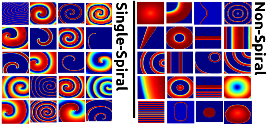
Figure 1: Collages of illustrative pseudocolor plots of $V$ with (a) single-spiral ($\mathscr{S}$) images and (b) no spiral ($\mathscr{NS}$) images, which we use for training our CNN. In (a), the arm-width of the spiral and its rotation frequency depends on the model [Eqs. (1) or (2)] and the parameters therein; the spiral-wave-initiation scheme controls the chirality of the spiral and the position of its core. In (b), the $\mathscr{NS}$ class includes plane waves and target waves.

Our solutions of Eqs. (1) or (2) yield $V$ at $N^{2}$ grid points. We first define the normalised transmembrane potential $\tilde{V}=(V-V_{min})/(V_{max}-V_{min})$; $V_{max}$ and $V_{min}$ are, respectively, the maximal and minimal values of $V$, so $0\leq\tilde{V}\leq 1$. We then reduce the large number of grid points by specifying $\tilde{V}$ on $32\times 32$ points by using the resize function in MATLAB R2018b. We use the Deep Learning Toolbox in MATLAB R2018b to develop our CNN, which we depict schematically in Fig. 2. It has three main layers: (1) Input; (2) Middle; and (3) Final. The Middle layer contains three sets of Convolution, Rectified Linear Unit (ReLU), and MaxPool sub-layers. The Final layer contains two fully connected Artificial Neural Networks (ANNs). We give a brief description of the implementation of our CNN in the Supplemental Material Supmat_Final_2019.

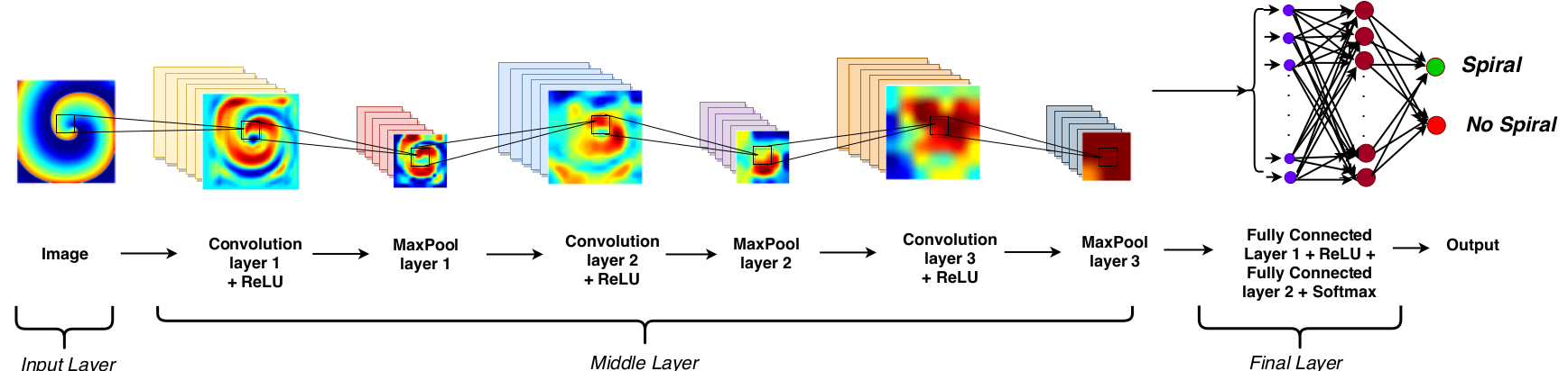
Figure 2: A schematic diagram of our CNN showing the Input, Middle, and Final layers; the details of each one of these layer are given in the Supplemental Material Supmat_Final_2019.

We begin the training by feeding the the image of $\tilde{V}$ to our CNN. If the CNN output predicts the class of the input image incorrectly, then we use a proxy cost function to rectify this error iteratively (until the CNN yields the correct output class). Specifically, we achieve this for our CNN by minimizing the cross-entropy cost function

$$\small{\mathcal{C}=-\sum_{\ell=1}^{M}\sum_{q=0}^{\eta-1}\frac{\large{[}O_{\ell,q}\ln(\tilde{O}_{\ell,q})+(1-O_{\ell,q})\ln(1-\tilde{O}_{\ell,q})\large{]}}{M}},$$ (3)

by using the stochastic-gradient-descent method with a learning rate $\alpha=0.001$ (see, e.g., Chapter 2 of Ref Nielsen (2015)); here, $\tilde{O}_{\ell,q}$ are the CNN outputs ($\tilde{O}_{\ell,q}\in(0,1)$) and $O_{\ell,q}$ are the real outputs, for the input image $\ell$, and $M$ is the mini-batch size (the total number of images is divided into subsets, called mini-batches, with $M$ images each); we use $M=128$. For the class $\mathscr{S}$, $O_{\ell,0}=1$ and $O_{\ell,1}=0$; and for $\mathscr{NS}$, $O_{\ell,0}=0$ and $O_{\ell,1}=1$.

Even though we train our CNN with single-spiral-wave patterns, it manages to identify patterns with broken spiral waves as belonging to the class $\mathscr{S}$: We have checked that this CNN classifies 10,000 broken-spiral-wave patterns (see the pseudocolor plot of $V$ in Fig.3 (a)) as $\mathscr{S}$, with an accuracy of $99.6\%$. This is especially useful when we carry out the mathematical analog of defibrillation, i.e., the elimination of all spirals, unbroken or broken. We can, indeed, utilise our trained CNN to examine pseudocolor plots of $V$, during our numerical simulation of a mathematical model for cardiac tissue; the moment this CNN detects a pattern of type $\mathscr{S}$, we can eliminate it by the application of suitable currents on a coarse, control mesh Sinha et al. (2001) or by using an optogenetics-based control Bingen et al. (2014) method (we give a brief description of these control methods (see Fig. S3) in the Supplemental Material Supmat_Final_2019). Here, we discuss a new scheme for eliminating both broken and unbroken spiral waves; this relies on developing a heat map, from a pseudocolor plot of $V$, for those images that are identified by our CNN to lie in the class $\mathscr{S}$. This heat map (Fig. 3 (b)) is

$$\mathcal{H}(i,j)=\frac{N_{p}}{N}\sum_{r=1}^{N/Np}{\rm CNN}\left(\chi^{r}_{i,j}\left\{V\right\}\right),$$ (4)

$\forall i,j\in\{1,2,\ldots,N\}$; the arguments of the matrix-resizing function $\chi^{r}_{i,j}$ (a standard function in Matlab) are the $32r\times 32r$ values of $V$ in a square of side $32r$ centred at the point $(i,j)$, with $1\leq i,j\leq N$ and $1\leq r\leq(N/N_{p})$; for the images we employ, $N=512$ and $N_{p}=32$. We use the resized $\chi^{r}_{i,j}$, an image with $N_{p}\times N_{p}$ pixels, as an input into our CNN (Fig. 2) and its output, $0$ (for $\mathscr{NS}$) or $1$ (for $\mathscr{S}$), is summed over $r$ to obtain $\mathcal{H}(i,j)$ for a given input pseudocolor plot of $V$. Clearly, $\mathcal{H}(i,j)\in[0,1]$; and it is large if there is a spiral core near the point $(i,j)$. In the left and right panels of Fig. 3 we depict, respectively, a pseudocolor plot of $V$, with a broken-spiral-wave pattern, and the corresponding heat map. We now show how to use such a heat map to develop a new control scheme for the elimination of both broken and unbroken spiral waves.

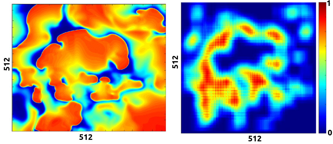
Figure 3: Pseudocolor plots of (left panel) $V$, showing broken spiral waves, and (right panel) the heat map $\mathcal{H}$ for the image in the left panel (see text).

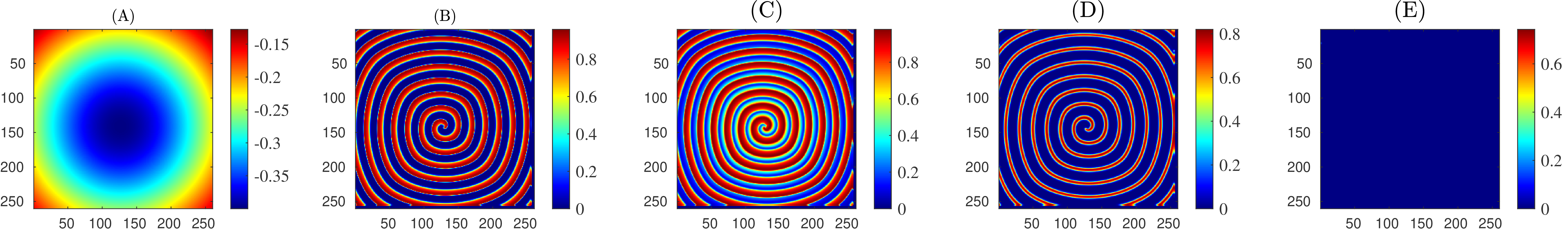
Figure 4: Pseudocolor plots which shows, (A) the defibrillation current as $\mathcal{P_{H}}$ (single 2D Gaussian centered at the spiral core), whose $I_{def}=0.5$ pA/pF, $\sigma=0.375N\Delta x$ (cm) and $N=256$. (B)-(F) $V$ of the Aliev-Panfilov model (Ref Aliev and Panfilov (1996)). (B) the spiral wave before application of the defibrillation current and (C) shows the time of application and (D)-(F) After the defibrillation current is applied. We observe that spiral wave is eliminated after the application of the defibrillaion current of 2D Gaussian profile.

Spiral-wave excitations emanate from the spiral core, so we might expect that the elimination of this core could lead to the removal of the spiral wave. However, when we apply a current pulse on a disk centred at the spiral core, we find that it leads to the formation of multiple spiral cores along the boundary of the disk. We prevent the formation of such multiple spiral cores as follows: We first show, for a single spiral wave in the Aliev-Panfilov model, that, by applying a current pulse with a spatial profile that is a symmetrical, two-dimensional (2D) Gaussian (centred at the spiral core, with equal widths in both $x$ and $y$ directions $\sigma_{x}=\sigma_{y}=\sigma$, and with a peak intensity of $I_{def}$), we can remove the core and the wave without forming multiple spiral cores (Fig. 4). Henceforth, we refer to such a current profile as a Gaussian current pulse with width $\sigma$.

We now consider a pattern with multiple spiral waves (e.g., the pseudocolor plot of $V$ in the left panel of Fig. 3), whose spatial extent is much smaller than the large spiral wave in Fig. 4. We consider a square lattice of points, labelled by $(i^{\prime},j^{\prime})$, with $0\leq i^{\prime},j^{\prime}\leq N_{G}$, i.e., the side of the unit cell $a=N_{G}\Delta x$ (cm). On each of these points we impose a Gaussian current pulse $G(i^{\prime},j^{\prime})$ of width $\sigma$ and amplitude $I_{def}$; the total, normalised contribution of these pulses, at the point $(i,j)$, with $0\leq i,j\leq(N-1)$, in the original image, is

$$\tilde{\mathcal{G}}(i,j) = \sum_{i^{\prime},j^{\prime}=0}^{N_{G}}G\left(i-i^{\prime}\frac{N}{N_{G}},j-j^{\prime}\frac{N}{N_{G}}\right);$$

$$\mathcal{G}(i,j) = \tilde{\mathcal{G}}(i,j)/[\tilde{\mathcal{G}}_{max}];$$ (5)

here, $\tilde{\mathcal{G}}_{max}=max_{(i,j)}[\tilde{\mathcal{G}}(i,j)]$. The final current pulse that we apply, for a time $t_{def}$ ms at the point $(i,j)$, is given by the Hadamard product

$$\mathcal{P_{H}}(i,j)=I_{def}\ \mathcal{H}(i,j)\mathcal{G}(i,j),$$ (6)

where $I_{def}$ sets the scale of the current that is applied. Multiple spiral waves are eliminated by the application of $\mathcal{P_{H}}(i,j)$ (henceforth, Gaussian-control scheme) as we demonstrate below.

In Figs. 5 (A) and (B), we show illustrative pseudocolor plots of, respectively, $V$ and its heat map $\mathcal{H}$ (Eq.( 4)), for an image with a broken spiral wave, in the TP06 model. Figures 5 (C) and (D) depict, respectively, pseudocolor plots of the summed and normalised 2D Gaussians ($\mathcal{G}(i,j)$ in Eq.( 5)) and the Hadamard product $\mathcal{P_{H}}(i,j)$ (with $I_{def}=1$ pA/pF in Eq.( 6)). Our Gaussian-control scheme is illustrated by the pseudocolor plots of $V$ [Figs. 5 (E)-(H)]; these show the spatiotemporal evolution of $V$ after the application of $\mathcal{P_{H}}(i,j)$, which is turned off at $t=t_{def}$ (for the complete spatiotemporal evolution see the video V1 in the Supplemental Material Supmat_Final_2019). In Figs. 5 (I)-(L) we show the counterparts of Figs. 5 (E)-(H) for the control scheme in which a current pulse is applied on a square mesh to eliminate broken spiral waves (see Refs. Sinha et al. (2001); Shajahan et al. (2007, 2009); Nayak and Pandit (2014), the Supplemental Material Supmat_Final_2019, and the video V2); we refer to this as the mesh-control scheme.

Control	$N_{G}$	$a$	$\sigma$	$I_{def}$	$t_{def}$
scheme		(cm)	(cm)	(pA/pF)	(ms)
GC1	64	1.6	0.37 $a$	5	120
GC2	96	2.4	0.37 $a$	5	120
MC	64	-	-	15	120

Table 1: The parameter values that we use for our Gaussian-control (GC1 and GC2) and Mesh-control (MC) schemes in our illustrative simulations.

The efficacy of our Gausssian-control scheme depends on the parameters $a,\,\sigma,\,I_{def}$, and $t_{def}$. We list these parameters (Table 1) for two illustrative Gaussian-control runs, GC1 and GC2, and one run, MC, in which we use a mesh-control scheme, for the TP06 model. By comparing the results of such runs we find that, for large values of $a$, our Gaussian-control scheme is not successful in removing spiral waves; e.g., in the TP06 model, broken spiral waves are suppressed for the value of $a$ that we use in run GC1, but not for the value of $a$ in run GC2 (Table 1). For the parameters in run GC1, Figs. 5 (M)-(P) show phase diagrams, in the $(t_{def},\sigma)$ plane and for representative values of $I_{def}$, with parameter regions in which our Gaussian-control scheme succeeds (red) and does not succeed (blue) in controlling broken spiral waves: This Gaussian-control scheme also eliminates broken and unbroken spiral waves in all the other cardiac-tissue models that we have studied (see Figs. S5 and S6 in the Supplemental Material Supmat_Final_2019).

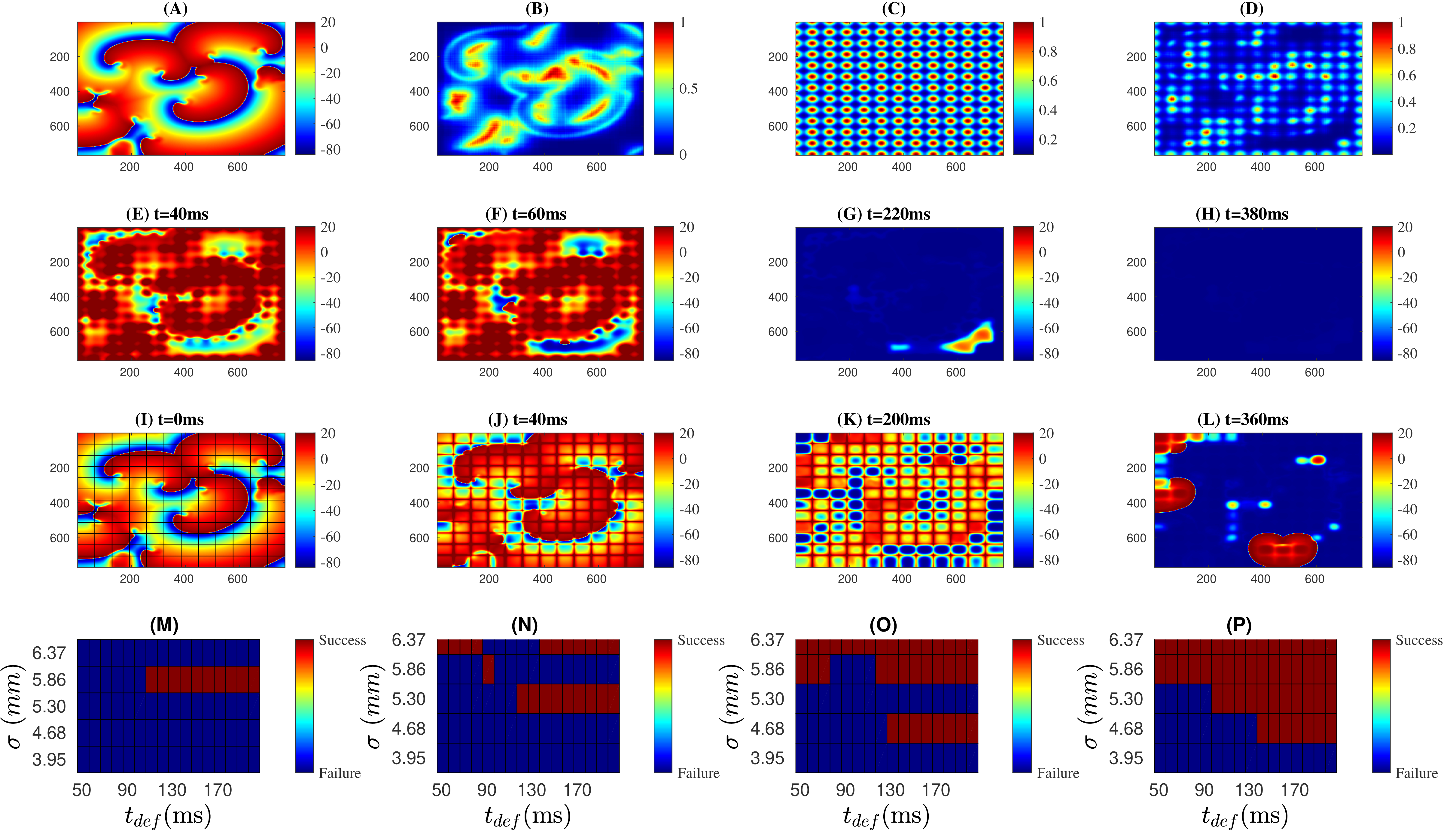
Figure 5: Pseudocolor plots of (A) $V$, for an illustrative, broken spiral wave from our simulation of the the TP06 model, (B) the corresponding heat map $\mathcal{H}$ (Eq. 4), (C) the summed and normalised 2D Gaussians ($\mathcal{G}(i,j)$ in Eq. 5), and (D) the Hadamard product $\mathcal{P_{H}}(i,j)$ (with $I_{def}=1$ pA/pF in Eq. 6). (E)-(H): Pseudocolor plots of $V$, at different representative times, showing the elimination of the broken spiral waves (as in (A) at $t=0$) after the application of $\mathcal{P_{H}}(i,j)$; $\mathcal{P_{H}}(i,j)$ is turned off at $t=t_{def}=120$ ms (for the complete spatiotemporal evolution see the video V1 in the Supplemental Material Supmat_Final_2019). (I)-(L): the analogs of (E)-(H) for the current-mesh control scheme of Refs. Sinha et al. (2001) (see the video V2 in Supplemental Material Supmat_Final_2019). Phase diagrams in the $(t_{def},\sigma)$ plane showing parameter regions in which our Gaussian control scheme [(E)-(F)] succeeds (red) and does not succeed (blue) in controlling broken spiral waves for (M) $I_{def}=5$ pA/pF, (N) $I_{def}=10$ pA/pF, (O) $I_{def}=15$ pA/pF and (P) $I_{def}=20$ pA/pF.

By comparing the pseudocolor plots in rows two and three of Fig. 5, we can contrast the effectivness of our Gaussian-control scheme with that of the mesh-control scheme of Refs Sinha et al. (2001). We find, in particular, that our Gaussian-control scheme eliminates broken spiral waves with $I_{def}=5$ pA/pF; by contrast, the mesh scheme requires $I_{def}=15$ pA/pF for such elimination. Thus, the Gaussian-control scheme leads to the elimination of spiral waves with lower local currents than the mesh-control scheme, with all other parameters held fixed.

We have checked that our CNN can be used to detect scroll waves in three-dimensional(3D) simulation domains (see Fig. S4 of the Supplimentary Material Ref Supmat_Final_2019). The elimination of such 3D scroll waves by the application of currents on a 2D surface of a 3D domain remains a significant challenge Ref. Sinha et al. (2001); Shajahan et al. (2007, 2009); Nayak and Pandit (2014).

Our deep-learning-assisted Gaussian-control method is an important step in the detection and elimination of both broken and unbroken spiral waves. Machine-learning techniques have been used, e.g., in Refs. Figuera et al. (2016); Maršánová et al. (2017); Hannun et al. (2019), for the effective detection of anomalies in electrocardiograms (ECGs), which can then be eliminated by the controlled delivery of electrical signals via automated defibrillators (see, e.g. Refs. Figuera et al. (2016); Singh et al. (2018); Ao Li and R ). To the best our of knowledge, no machine-learning method has been employed so far for the detection of spiral waves in, e.g., pseudocolor plots of $V$. Our study uses the complete spatial information in patterns of $V$ to develop an efficient Gaussian-control scheme for the elimnation of unbroken and broken spiral waves, which are the mathematical analogs of life-threatening VT and VF Shajahan et al. (2007, 2009); Nayak and Pandit (2014).

We hope that our CNN-based detection of spiral waves and our Gaussian-control scheme will be tested in in-vitro experiments with cardiac myocytes, such as those used in the studies of Refs. Davidenko et al. (1990); Ikeda et al. (1996); Valderrábano et al. (2000); Lim et al. (2006); Bingen et al. (2014); Shajahan et al. (2016); Kudryashova et al. (2017). Our CNN can also be used to detect spiral waves in other excitable media Lechleiter et al. (1991); Winfree (1972); Falcke et al. (1992); Imbihl and Ertl (1995); Pande and Pandit (1999); Marino and Giacomelli (2019); Tyson and Murray (1989); Rietdorf et al. (1996).

References

- Mehra (2007) R. Mehra, Journal of electrocardiology 40, S118 (2007).
- Majumder et al. (2011) R. Majumder, A. R. Nayak, and R. Pandit, An Overview of Spiral- and Scroll-Wave Dynamics in Mathematical Models for Cardiac Tissue (Springer Berlin Heidelberg, Berlin, Heidelberg, 2011), pp. 269–282, ISBN 978-3-642-17575-6, URL https://doi.org/10.1007/978-3-642-17575-6_14.
- Clayton et al. (2011) R. Clayton, O. Bernus, E. Cherry, H. Dierckx, F. H. Fenton, L. Mirabella, A. V. Panfilov, F. B. Sachse, G. Seemann, and H. Zhang, Progress in biophysics and molecular biology 104, 22 (2011).
- Honnekeri et al. (2014) B. S. Honnekeri, D. Lokhandwala, G. K. Panicker, and Y. Lokhandwala, J Assoc Physicians India 62, 36 (2014).
- Zheng et al. (2001) Z.-J. Zheng, J. B. Croft, W. H. Giles, and G. A. Mensah, Circulation 104, 2158 (2001).
- Berul et al. (1996) C. I. Berul, M. J. Aronovitz, P. J. Wang, and M. E. Mendelsohn, Circulation 94, 2641 (1996).
- Chinushi et al. (2003) M. Chinushi, D. Kozhevnikov, E. B. Caref, M. Restivo, and N. El-Sherif, Journal of cardiovascular electrophysiology 14, 632 (2003).
- Gelzer et al. (2008) A. R. Gelzer, M. L. Koller, N. F. Otani, J. J. Fox, M. W. Enyeart, G. J. Hooker, M. L. Riccio, C. R. Bartoli, and R. F. Gilmour, Circulation 118, 1123 (2008).
- Davidenko et al. (1990) J. M. Davidenko, P. F. Kent, D. R. Chialvo, D. C. Michaels, and J. Jalife, Proceedings of the National Academy of Sciences 87, 8785 (1990).
- Ikeda et al. (1996) T. Ikeda, T. Uchida, D. Hough, J. J. Lee, M. C. Fishbein, W. J. Mandel, P.-S. Chen, and H. S. Karagueuzian, Circulation 94, 1962 (1996).
- Valderrábano et al. (2000) M. Valderrábano, Y.-H. Kim, M. Yashima, T.-J. Wu, H. S. Karagueuzian, and P.-S. Chen, Journal of the American College of Cardiology 36 (2000).
- Lim et al. (2006) Z. Y. Lim, B. Maskara, F. Aguel, R. Emokpae, and L. Tung, Circulation 114, 2113 (2006).
- Shajahan et al. (2007) T. Shajahan, S. Sinha, and R. Pandit, Physical Review E 75, 011929 (2007).
- Shajahan et al. (2009) T. Shajahan, A. R. Nayak, and R. Pandit, PLoS One 4, e4738 (2009).
- Nayak and Pandit (2014) A. R. Nayak and R. Pandit, Frontiers in physiology 5, 207 (2014).
- Moreno et al. (2013) J. Moreno, P.-C. Yang, J. Bankston, E. Grandi, D. Bers, R. Kass, and C. Clancy, Circulation research pp. CIRCRESAHA–113 (2013).
- Sinha et al. (2001) S. Sinha, A. Pande, and R. Pandit, Physical review letters 86, 3678 (2001).
- Luther et al. (2011) S. Luther, F. H. Fenton, B. G. Kornreich, A. Squires, P. Bittihn, D. Hornung, M. Zabel, J. Flanders, A. Gladuli, L. Campoy, et al., Nature 475, 235 (2011).
- Bingen et al. (2014) B. O. Bingen, M. C. Engels, M. J. Schalij, W. Jangsangthong, Z. Neshati, I. Feola, D. L. Ypey, S. F. Askar, A. V. Panfilov, D. A. Pijnappels, et al., Cardiovascular research 104, 194 (2014).
- Lechleiter et al. (1991) J. Lechleiter, S. Girard, E. Peralta, and D. Clapham, Science 252, 123 (1991).
- Winfree (1972) A. T. Winfree, Science 175, 634 (1972).
- Falcke et al. (1992) M. Falcke, M. Bär, H. Engel, and M. Eiswirth, The Journal of chemical physics 97, 4555 (1992).
- Imbihl and Ertl (1995) R. Imbihl and G. Ertl, Chemical Reviews 95, 697 (1995).
- Pande and Pandit (1999) A. Pande and R. Pandit (1999).
- Marino and Giacomelli (2019) F. Marino and G. Giacomelli, Physical Review Letters 122, 174102 (2019).
- Tyson and Murray (1989) J. J. Tyson and J. Murray, Development 106, 421 (1989).
- Rietdorf et al. (1996) J. Rietdorf, F. Siegert, and C. J. Weijer, Developmental biology 177, 427 (1996).
- Barkley (1991) D. Barkley, Physica D: Nonlinear Phenomena 49, 61 (1991).
- Aliev and Panfilov (1996) R. R. Aliev and A. V. Panfilov, Chaos, Solitons & Fractals 7, 293 (1996).
- Luo and Rudy (1991) C.-h. Luo and Y. Rudy, Circulation research 68, 1501 (1991).
- Ten Tusscher and Panfilov (2006) K. H. Ten Tusscher and A. V. Panfilov, American Journal of Physiology-Heart and Circulatory Physiology 291, H1088 (2006).
- O’Hara et al. (2011) T. O’Hara, L. Virág, A. Varró, and Y. Rudy, PLoS computational biology 7, e1002061 (2011).
- Press et al. (2007) W. H. Press, S. A. Teukolsky, W. T. Vetterling, and B. P. Flannery, Numerical recipies 3rd edition: the art of scientific computing (2007).
- Nielsen (2015) M. A. Nielsen, Neural networks and deep learning, vol. 25 (Determination press USA, 2015).
- Figuera et al. (2016) C. Figuera, U. Irusta, E. Morgado, E. Aramendi, U. Ayala, L. Wik, J. Kramer-Johansen, T. Eftestøl, and F. Alonso-Atienza, PloS one 11, e0159654 (2016).
- Maršánová et al. (2017) L. Maršánová, M. Ronzhina, R. Smíšek, M. Vítek, A. Němcová, L. Smital, and M. Nováková, Scientific reports 7, 11239 (2017).
- Hannun et al. (2019) A. Y. Hannun, P. Rajpurkar, M. Haghpanahi, G. H. Tison, C. Bourn, M. P. Turakhia, and A. Y. Ng, Nature medicine 25, 65 (2019).
- Singh et al. (2018) S. Singh, S. K. Pandey, U. Pawar, and R. R. Janghel, Procedia Computer Science 132, 1290 (2018).
- (39) S. C. Ao Li and J. M. R, Res Med Eng Sci. 4(4). RMES.000592.2018.DOI: 10.31031/RMES.2018.04.000592 (????).
- Shajahan et al. (2016) T. Shajahan, S. Berg, S. Luther, V. Krinski, and P. Bittihn, New Journal of Physics 18, 043012 (2016).
- Kudryashova et al. (2017) N. Kudryashova, V. Tsvelaya, K. Agladze, and A. Panfilov, Scientific reports 7, 7887 (2017).