Meta Reinforcement Learning with Task Embedding and Shared Policy

Abstract

Despite significant progress, deep reinforcement learning (RL) suffers from data-inefficiency and limited generalization. Recent efforts apply meta-learning to learn a meta-learner from a set of RL tasks such that a novel but related task could be solved quickly. Though specific in some ways, different tasks in meta-RL are generally similar at a high level. However, most meta-RL methods do not explicitly and adequately model the specific and shared information among different tasks, which limits their ability to learn training tasks and to generalize to novel tasks. In this paper, we propose to capture the shared information on the one hand and meta-learn how to quickly abstract the specific information about a task on the other hand. Methodologically, we train an SGD meta-learner to quickly optimize a task encoder for each task, which generates a task embedding based on past experience. Meanwhile, we learn a policy which is shared across all tasks and conditioned on task embeddings. Empirical results on four simulated tasks demonstrate that our method has better learning capacity on both training and novel tasks and attains up to 3 to 4 times higher returns compared to baselines.

1 Introduction

Reinforcement learning (RL) aims to guide an agent to take actions in an environment such that the cumulative reward is maximized Sutton et al. (1998). Recently, deep RL has achieved great progress in applications such as AlphaGo Silver et al. (2016), playing Atari games Mnih et al. (2013), and robotic control Levine et al. (2016) by using deep neural networks. However, existing RL methods suffer from data-inefficiency and limited generalization, since they learn each task from scratch without reusing past experience, even though these tasks are quite similar. Recent progress in meta-learning has shown its power to solve few-shot classification problems Finn et al. (2017); Snell et al. (2017), which can learn a model for a novel few-shot classification task in just a few iterations. In this paper, we further investigate to apply meta-learning to RL domains (called meta-RL).

Basically, meta-RL consists of two modules: policy and meta-learner. The former defines the network structure mapping observations to actions, and the latter is applied to optimize a policy (i.e., learn a set of parameters) for each task. The objective of meta-RL is to train a meta-learner from a set of RL tasks, which can quickly optimize a policy to solve a novel but related task. In effect, meta-RL explores how to solve a family of tasks rather than a single task as in conventional RL.

A major limitation of most meta-RL methods (discussed thoroughly in § 2) is that they do not explicitly and adequately model the individuality and the commonness of tasks, which has proven to play an important role in the literature of multi-task learning Ruder (2017); Ma et al. (2018) and should be likewise applicable to meta-RL. Take the case of locomotion tasks, where an agent needs to move to different target locations for different tasks. The nature of this type of tasks (i.e., the commonness) is the way to control the agent to move from one location to another, and different tasks are mainly distinguished by the corresponding target locations (i.e., the individuality). Humans have a similar mechanism to solve such decision making problems. Imagine that when we want to walk to some different places, we do not need to modify the method we walk, but modify the destinations we want to go. Therefore, we hypothesize that a more principled approach for meta-RL is to characterize the commonness of all tasks on the one hand and meta-learn how to quickly abstract the individuality of each task on the other hand.

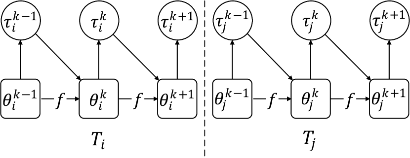
(a) MAML Finn et al. (2017).

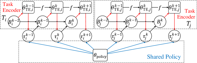
(b) TESP.

Figure 1: Computation graphs of MAML and TESP. (1(a)) The meta-learner $f$ of MAML optimizes a policy $\theta_{i}$ for each task $T_{i}$ via standard policy gradient using sampled episodes $\tau_{i}$. (1(b)) TESP trains a meta-learner $f$ and a shared policy. The meta-learner optimizes a task encoder (TE) $\theta_{\text{TE},i}$ for each task $T_{i}$ based on previously sampled episodes stored in the episode buffer $B_{i}$. The policy $\theta_{\text{policy}}$ is shared across tasks and accomplishes a task based on observations and the output of the corresponding task encoder.

Based on the above motivation, we introduce a new component into the current meta-RL framework, named task encoder, and develop a new meta-RL method, which achieves better performance on both training and novel tasks with Task Encoder adaptation and Shared Policy, namely TESP. Figure 1 illustrates the computation graph of TESP. Instead of training a meta-learner that directly optimizes a policy for each task (i.e., policy adaptation), TESP trains a meta-learner to quickly optimize a task encoder for each task (i.e., task encoder adaptation). The task-specific encoder generates a latent task embedding based on past experience (i.e., previously explored episodes) stored in an episode buffer. At the same time, TESP trains a shared policy across different tasks. The shared policy is conditioned on task embeddings, which allows to accomplish different tasks based on the corresponding task embeddings with the same set of policy parameters.

The main idea behind TESP is that we apply the meta-learner to quickly abstract the individuality of each task via task encoder adaptation, and the shared policy characterizes the commonness of a family of tasks. We evaluate our method on a variety of simulated tasks: locomotion with a wheeled agent, locomotion with a quadrupedal agent, 2-link reacher, and 4-link reacher. Empirical results show that our method has better learning capacity on both training and novel tasks.

2 Related Work

The works most related to ours are MAML Finn et al. (2017) and Meta-SGD Li et al. (2017). Specifically, MAML trains a parametrized stochastic gradient descent (SGD) optimizer as the meta-learner, which is expected to have a good network initialization such that different tasks can be learned quickly with vanilla policy gradient (VPG) Williams (1992). Meta-SGD further extends MAML by introducing adaptive per-parameter learning rates. To a certain extent, the initialization and adaptive learning rates encode the commonness of different tasks. However, the task-specific information (i.e., the individuality) can only be implicitly obtained through subsequent policy gradient update, which is sparse and delayed, and not effective enough for exploration in RL. In contrast, we introduce a meta-learned task encoder to explicitly abstract the individuality of each task represented by a task embedding. For each task, the task embedding is then fed into a policy network at each timestep, which leads to dense and immediate task-specific guidance. On the other hand, we encoder the commonness of a kind of tasks into a shared policy, rather than the parameters of the SGD optimizer.

Another related work is MAESN Gupta et al. (2018b), which additionally meta-learns a latent variable to capture the task-specific information based on MAML. The variable is fed into a policy network and held constant over the duration of episodes as well. However, we observe that simply adapting a single variable is not enough to represent a task in our experiments (conducted in a more challenging way than Gupta et al. (2018b)). Meanwhile, there are some hierarchical RL (HRL) works that involve optimizing a latent variable and have a similar network architecture to TESP. For example, Florensa et al. (2017) pre-learns a policy conditioned on skills represented by a latent variable $z$, and uses the pre-learned policy conditioned on task-specific skills to learn different tasks. The task-specific skills are obtained by training extra neural networks with $z$ as input. The latent variables learned by the above works can also be regarded as task embeddings, which, to some extent, are learned in a transductive-like way. The key difference is that our method tries to induce a general function to acquire task embeddings from episodes that have been experienced in the past, which should be more generalizable to novel tasks. On the other hand, conventional HRL methods usually cannot learn novel tasks quickly (e.g., in $3$ iterations).

MLSH Frans et al. (2018) also introduces the concept of “shared policy”, which learns a set of shared policies across all tasks and meta-learns a master policy to choose different policies in different time periods for each task. We think TESP and MLSH are developed from different perspectives and should be complementary to each other. In particular, TESP can be further extended with a set of shared conditional policies, which we leave as future work. On the other hand, the master policy of MLSH makes decisions based on observations, which could be further improved by conditioning on a task embedding output by a (meta-learned) task encoder.

Another line of work is to use a recurrent architecture to act as the meta-learner. For instance, Duan et al. (2016) meta-learns a recurrent neural network (RNN) which learns a task by updating the hidden state via the rollout and preserving the hidden state across episode boundaries. Mishra et al. (2017) further designs a more complex recurrent architecture based on temporal convolutions and soft attention. These methods encode the task individuality into the internal state of the meta-learner (e.g., the hidden state of RNN). However, depending on the feed-forward calculation to learn a task seems to lead to completely overfitting to the distribution of training tasks and fail to learn novel tasks sampled from a different distribution as shown in Houthooft et al. (2018). Some prior works Kang and Feng (2018); Tirinzoni et al. (2018) show that MAML also suffers from this problem to some extent.

Other recent works mainly explore meta-RL from different perspectives about what to meta-learn, such as the exploration ability Stadie et al. (2018), the replay buffer for training DDPG Lillicrap et al. (2015); Xu et al. (2018b), non-stationary dynamics Al-Shedivat et al. (2017), factors of temporal difference Xu et al. (2018c), the loss function Houthooft et al. (2018), the environment model for model-based RL Clavera et al. (2018), and the reward functions in the context of unsupervised learning and inverse RL respectively Gupta et al. (2018a); Xu et al. (2018a). Interested readers could refer to the reference citations for more details.

3 Preliminaries

In this section, we first formally define the problem of meta-RL, and then introduce a typical meta-learning (or meta-RL) method, MAML Finn et al. (2017), for consistency.

3.1 Meta-RL

In meta-RL, we consider a set of tasks $D$, of which each is a Markov decision process (MDP). We denote each task by $T_{i}=(S,A,H,P_{i},r_{i})$, where $S$ is the state space , $A$ is the action space, $H$ is the horizon (i.e., the maximum length of an episode), $P_{i}\colon S\times A\times S\to\mathbb{R}_{\geqslant 0}$ is the transition probability distribution, and $r_{i}\colon S\times A\to\mathbb{R}$ is the reward function. Tasks have the same state space, action space, and horizon, while the transition probabilities and reward functions differ across tasks.

Given the state $s_{i,t}\in S$ perceived from the environment at time $t$ for task $T_{i}$, a policy $\pi_{\theta_{i}}\colon S\times A\to\mathbb{R}_{\geqslant 0}$, parametrized by $\theta_{i}$, predicts a distribution of actions, from which an action $a_{i,t}\sim\pi_{\theta_{i}}(a_{i,t}|s_{i,t})$ is sampled. The agent moves to the next state $s_{i,t+1}\sim P_{i}(s_{i,t+1}|s_{i,t},a_{i,t})$, and receives an immediate reward $r_{i,t}=r_{i}(s_{i,t},a_{i,t})$. As the agent repeatedly interacts with the environment, an episode $\tau_{i}=(s_{i,0},a_{i,0},r_{i,0},...,s_{i,t},a_{i,t},r_{i,t},...)$ is collected, and it stops when the termination condition is reached or the length of $\tau_{i}$ is $H$. We denote by $\tau_{i}\sim P_{i}(\tau_{i}|\theta_{i})$ sampling an episode $\tau_{i}$ under $\pi_{\theta_{i}}$ for task $T_{i}$. In general, the goal of meta-RL is to train a meta-learner $f$, which can quickly learn a policy (i.e., optimizing the parameter $\theta_{i}$) to minimize the negative expected reward for each task $T_{i}\in D$:

$$L_{T_{i}}(\tau_{i}|\theta_{i})=-\mathbb{E}_{\tau_{i}\sim P_{i}(\tau_{i}|\theta_{i})}[R(\tau_{i})]$$ (1)

where $R(\tau_{i})=\sum_{t}r_{i,t}$.

Basically, the training procedure of meta-RL consists of two alternate stages: fast-update and meta-update. During fast-update, the meta-learner runs optimization several times (e.g., $3$ times) to obtain an adapted policy for each task. During meta-update, the meta-learner is optimized to minimize the total loss of all tasks under the corresponding adapted policies.

3.2 MAML

Different meta-RL methods mainly differ in the design of the meta-learner and fast-update. Here, we will give a brief introduction with MAML Finn et al. (2017) as an example. The computation graph of MAML is shown in Figure 1(a).

MAML trains an SGD optimizer, parametrized by $\theta$, as the meta-learner. During fast-update, for each task $T_{i}\in D$, the meta-learner first initializes a policy network with $\theta_{i}^{1}=\theta$, and then performs VPG update $K$ times. The fast-update stage is formulated as follows:

$$\theta_{i}^{k+1}=\theta_{i}^{k}-\alpha\nabla_{\theta_{i}^{k}}L_{T_{i}}(\tau_{i}^{k}|\theta_{i}^{k}),\quad k=1,\ldots,K$$ (2)

where $\alpha$ is the learning rate and $K$ is the number of fast-updates. Combined with meta-update, MAML aims to learn a good policy initialization, from which different parameters can be quickly learned for different tasks.

4 Algorithm

In this section, we propose a new meta-RL method TESP that explicitly models the individuality and commonness of tasks. Specifically, TESP learns a shared policy to characterize the task commonness, and simultaneously trains a meta-learner to quickly abstract the individuality to enable the shared policy to accomplish different tasks. We will first introduce the overall network architecture of TESP, and then elaborate how to leverage this architecture in a meta-learning manner.

4.1 Network Architecture

Here, we first introduce the network structure of TESP composed of a task encoder and a policy network, which is illustrated in Figure 2.

4.1.1 Task Encoder

The task encoder maps each task into a low-dimensional latent space. It is expected that the low-dimensional space $\mathbb{R}^{d}$ can capture differences among tasks, such that we can represent the individuality of each task using a low-dimensional vector $h\in\mathbb{R}^{d}$ named task embedding. The first question is what kind of information we can use to learn such a low-dimensional space. In RL, an agent explores in an environment and generates a bundle of episodes. Obviously, these episodes contain characteristics of the ongoing task which can be used to abstract some specific information about the task.

Therefore, let us denote the task encoder by $g\colon E\to\mathbb{R}^{d}$, where $E$ indicates the set of all episodes that an agent has experienced in an environment. However, simply using all episodes is computationally intensive in practice, because we usually sample dozens of (e.g., 32) episodes at each iteration and the size of $E$ will increase rapidly. Considering that our goal is to learn a discriminative embedding to characterize a task, the episodes with low rewards are helpless or even harmful as shown in § 5.3. To accelerate and boost the learning process, we propose to build an episode buffer $B_{i}$ for each task $T_{i}\in D$, which stores the best $M$ episodes an agent has experienced. Mathematically, we initialize the buffer as an empty set $B_{i}^{0}=\varnothing$, and then update the episode buffer as follows:

$$B_{i}^{k}=S_{M}(B_{i}^{k-1}\cup\{\tau_{i,1}^{k},\ldots,\tau_{i,N}^{k}\}),\quad k=1,2,\ldots,$$ (3)

where $B_{i}^{k}$ is the episode buffer after the $k\textsuperscript{th}$ iteration, $\tau_{i,\ast}^{k}$ is the episodes sampled at the $k^{\text{th}}$ iteration, $N$ is the number of episodes sampled at each iteration, and $S_{M}$ is a function that selects the best $M$ ($M<N$) episodes in terms of rewards:

$$S_{M}(X)=\operatorname*{arg\,max}_{X^{\prime}\subset X,|X^{\prime}|=M}\sum_{\tau\in X^{\prime}}R(\tau).$$ (4)

Furthermore, we use the episodes in the buffer to abstract the individuality of each task, as shown in Figure 2. Mathematically, we have

$$h_{i}^{k}=\frac{1}{M}\sum_{\tau\in B_{i}^{k-1}}g(\tau),\quad k=1,2,\ldots,$$ (5)

where $g(\tau)$ refers to modeling an episode using the task encoder and $h_{i}^{k}$ is the task embedding of task $T_{i}$ after the exploration of the $(k-1)^{\text{th}}$ iteration (or before the exploration of the $k^{\text{th}}$ iteration). Although a more principled way could be to design a more comprehensive mechanism to effectively and efficiently utilize all previously sampled episodes, we empirically find that the simple episode buffer can achieve good enough performance, and we leave it as future work.

Given that an episode is a sequence of triplets $(s_{t},a_{t},r_{t})$, we model the task encoder $g$ as an RNN with GRU cell followed by a fully-connected layer. At each timestep, the GRU cell receives the concatenation of state, action, and reward as shown in Figure 2.

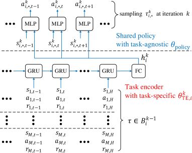
Figure 2: Network architecture of TESP composed of a task encoder (an RNN with GRU cell followed by a fully-connected (FC) layer) and a policy network (an MLP network). For each task $T_{i}$, when sampling episodes $\tau_{i,*}^{k}$ at the $k\textsuperscript{th}$ iteration (or fast-update), the task encoder first uses experienced episodes stored in the episode buffer $\tau\in B_{i}^{k-1}$ to calculate the corresponding task embedding $h_{i}^{k}$. Then, the embedding $h_{i}^{k}$, along with the observation, is passed into the MLP network to predict a distribution of actions at each timestep.

4.1.2 Policy

The policy $\pi$ predicts a distribution of actions based on the input. Since we have modeled each task using the corresponding task embedding, an agent can make decisions conditioned on the task-specific knowledge in addition to raw observations. Mathematically, we sample an episode $\tau_{i}^{k}$ for task $T_{i}$ at the $k^{\text{th}}$ iteration:

$$\tau_{i}^{k}\sim\pi(\tau_{i}^{k}|h_{i}^{k}).$$ (6)

At each timestep, the action is sampled as

$$a_{i,t}^{k}\sim\pi(a_{i,t}^{k}|[s_{i,t}^{k},h_{i}^{k}]),$$ (7)

where the input is the concatenation of the current observation and the task embedding of $T_{i}$. Note that $h_{i}^{k}$ represents the agent’s understanding of task $T_{i}$, and thus is appended to each timestep of the sampling at the $k^{\text{th}}$ iteration.

4.2 Meta-Learning

As mentioned before, we aim to quickly learn some discriminative information (i.e., the individuality) about a task, and model the commonness of a kind of tasks. For the individuality, inspired by MAML Finn et al. (2017), we propose to train an SGD optimizer (i.e., the meta-learner) to quickly learn a task encoder $g_{i}$ for each task $T_{i}\in D$, which further generates the corresponding task embedding. For the commonness, we propose to learn a policy, which is shared across different tasks. The shared policy is conditioned on task-specific embeddings, which allows to accomplish different tasks with the same policy parameters.

While an alternative for the individuality is to simply learn a single task encoder and use the same set of parameters to obtain task embeddings of different tasks based on the corresponding episode buffers, we find that it poorly generalizes to novel tasks as shown in § 5.3.

The parameters involved in TESP include

$$\theta=\{\theta_{\text{TE}},\alpha,\theta_{\text{policy}}\},$$ (8)

where $\theta_{\text{TE}}$ and $\alpha$ are the initialization and the learning rate of the SGD optimizer, and $\theta_{\text{policy}}$ is the parameter of the shared policy. Empirically, we use adaptive per-parameter learning rates $\alpha$, which has been found to have better performance than a fixed learning rate, as in some prior works Li et al. (2017); Al-Shedivat et al. (2017); Gupta et al. (2018b).

4.2.1 Fast-update

The purpose of the fast-update is to quickly optimize a task encoder $g_{i}$ for each task $T_{i}$ and obtain the corresponding task embedding, which is formulated as

$$\theta_{\text{TE},i}^{k+1}=\theta_{\text{TE},i}^{k}-\alpha\circ\nabla_{\theta_{\text{TE},i}^{k}}L_{T_{i}}(\tau_{i}^{k}|\theta_{i}^{k}),\quad k=1,\ldots,K.$$ (9)

Here, $\theta_{\text{TE},i}^{1}=\theta_{\text{TE}}$, $K$ is the number of fast-updates, $\circ$ denotes Hadamard product, and the definition of $L_{T_{i}}$ is the same as Eq. (1). Due to that the episode buffer is empty at the beginning, to make the derivation feasible at the first iteration, we first warm up the episode buffer by sampling a bundle of episodes $\tau_{i}^{\text{warm}}$ with the task embedding $h_{i}^{\text{warm}}$ assigned to a zero vector, and then calculate $h_{i}^{1}$ and sample episodes $\tau_{i}^{1}$.

Algorithm 1 Training Procedure of TESP

0:  training tasks $D$ and the number of fast-updates $K$

0:  the meta-learner $\theta_{\text{TE}},\alpha$ and the shared policy $\theta_{\text{policy}}$

1:  Randomly initialize $\theta_{\text{TE}}$, $\alpha$, and $\theta_{\text{policy}}$

2:  while not done do

3:    Sample a batch of tasks $T_{i}\in D$

4:    for all $T_{i}$ do

5:       Initialize $\theta_{i}^{1}=\{\theta_{\text{TE}},\alpha,\theta_{\text{policy}}\}$

6:       Sample episodes $\tau_{i}^{\text{warm}}$ with $h_{i}^{\text{warm}}=\vec{0}$, and warm up $B_{i}^{0}=S_{M}(\{\tau_{i,1}^{\text{warm}},\ldots,\tau_{i,N}^{\text{warm}}\})$

7:       for $k\in\{1,\ldots,K\}$ do

8:          Calculate task embedding $h_{i}^{k}$ via Eq. (5) using $\theta_{\text{TE},i}^{k}$

9:          Sample episodes $\tau_{i}^{k}$ using $h_{i}^{k}$ and $\theta_{\text{policy}}$

10:          Perform fast-update $\theta_{\text{TE},i}^{k+1}=\theta_{\text{TE},i}^{k}-\alpha\circ\nabla_{\theta_{\text{TE},i}^{k}}L_{T_{i}}(\tau_{i}^{k}|\theta_{i}^{k})$

11:          Update the episode buffer $B_{i}^{k}=S_{M}(B_{i}^{k-1}\cup\{\tau_{i,1}^{k},\ldots,\tau_{i,N}^{k}\})$

12:       end for

13:       Calculate task embedding $h_{i}^{K+1}$, and sample episodes $\tau_{i}^{K+1}$ using $h_{i}^{K+1}$ and $\theta_{\text{policy}}$

14:    end for

15:    Update $\theta_{\text{TE}}$, $\alpha$, and $\theta_{\text{policy}}$ to optimize the objective function (10)

16:  end while

4.2.2 Meta-update

During meta-update, we optimize the parameters of the SGD optimizer and the policy together to minimize the following objective function:

where $\eta>0$ is a constant factor that balances the effects of the two terms. Here, we propose to improve the generalization ability from two aspects: (1) The parameter $\theta_{\text{policy}}$ is only optimized w.r.t. all tasks during meta-update (without adaptation during fast-update), which enforces that a versatile policy is learned; (2) The second term in Eq. (10) acts as a regularizer to constrain that task embeddings of different tasks are not so far from the origin point such that the shared policy cannot learn to cheat. This term is inspired by VAE Kingma and Welling (2013), where the KL divergence between the learned distribution and a normal distribution should be small. We perform ablation studies on these two aspects in § 5.3. A concise training procedure is provided in Algorithm 1.

4.2.3 Adaptation to Novel Tasks

At testing time, we have a set of novel tasks, and expect to learn these tasks as efficiently as possible. We have obtained an SGD optimizer and a shared policy. The SGD optimizer is able to quickly learn a task encoder to abstract the individuality of a task represented by a task embedding, and the shared policy is able to accomplish different tasks conditioned on different task embeddings. Therefore, for each novel task, we simply sample episodes and employ the SGD optimizer to learn a task encoder to acquire the appropriate task embedding $h_{i}$ according to Eq. (5) and (9), while the policy does not need further adaptation.

5 Experiments

In this section, we comparatively evaluate our proposed method on four tasks with MuJoCo simulator Todorov et al. (2012): (1) a wheeled agent attempting to reach different target locations, (2) a quadrupedal ant attempting to reach different target locations, (3) a 2-link reacher attempting to reach different end-effector target locations, (4) a 4-link reacher attempting to reach different end-effector target locations. Figure 3 shows the renderings of agents used in the above tasks.

5.1 Experimental Settings

For each family of tasks, we sample $100$ target locations within a circle $\rho<R_{1}$ as training tasks $D$. When it comes to testing, we consider two scenarios: (1) Sample another $100$ target locations within the circle $\rho<R_{1}$ as novel/testing tasks $D^{\prime}$ (i.e., from the same distribution); (2) Sample $100$ target locations within an annulus $R_{1}<\rho<R_{2}$ as novel tasks $D^{\prime\prime}$ (i.e., from a different distribution). The wheeled and ant agents always start from the origin point, and the reachers are placed along the horizontal direction at the beginning.

We compare TESP with three baselines: MAML Finn et al. (2017), Meta-SGD Li et al. (2017), and TESP with a single variable being optimized during fast-update (denoted by AdaptSV) analogously to MAESN Gupta et al. (2018b). Here, we did not consider recurrent meta-learners such as RL² Duan et al. (2016) and SNAIL Mishra et al. (2017), due to that prior works have shown that recurrent meta-learners tend to completely overfit to the distribution of training tasks and cannot generalize to out-of-distribution tasks (i.e., $D^{\prime\prime}$ in this paper). We did not include some traditional HRL baselines that have a similar architecture to our method, because they are generally not suitable to our scenarios where we consider fast learning on novel tasks. For example, Florensa et al. (2017) requires training an extra neural network from scratch when learning a novel task, which is almost impossible to converge in $3$ iterations.

For each method, we set the number of fast-updates $K$ to $3$, and use the first-order approximation during fast-update to speed up the learning process as mentioned in Finn et al. (2017). We use VPG Williams (1992) to perform fast-update, and PPO Schulman et al. (2017) to perform meta-update. For detailed settings of environments and experiments, please refer to the supplement at https://github.com/llan-ml/tesp.

(a)

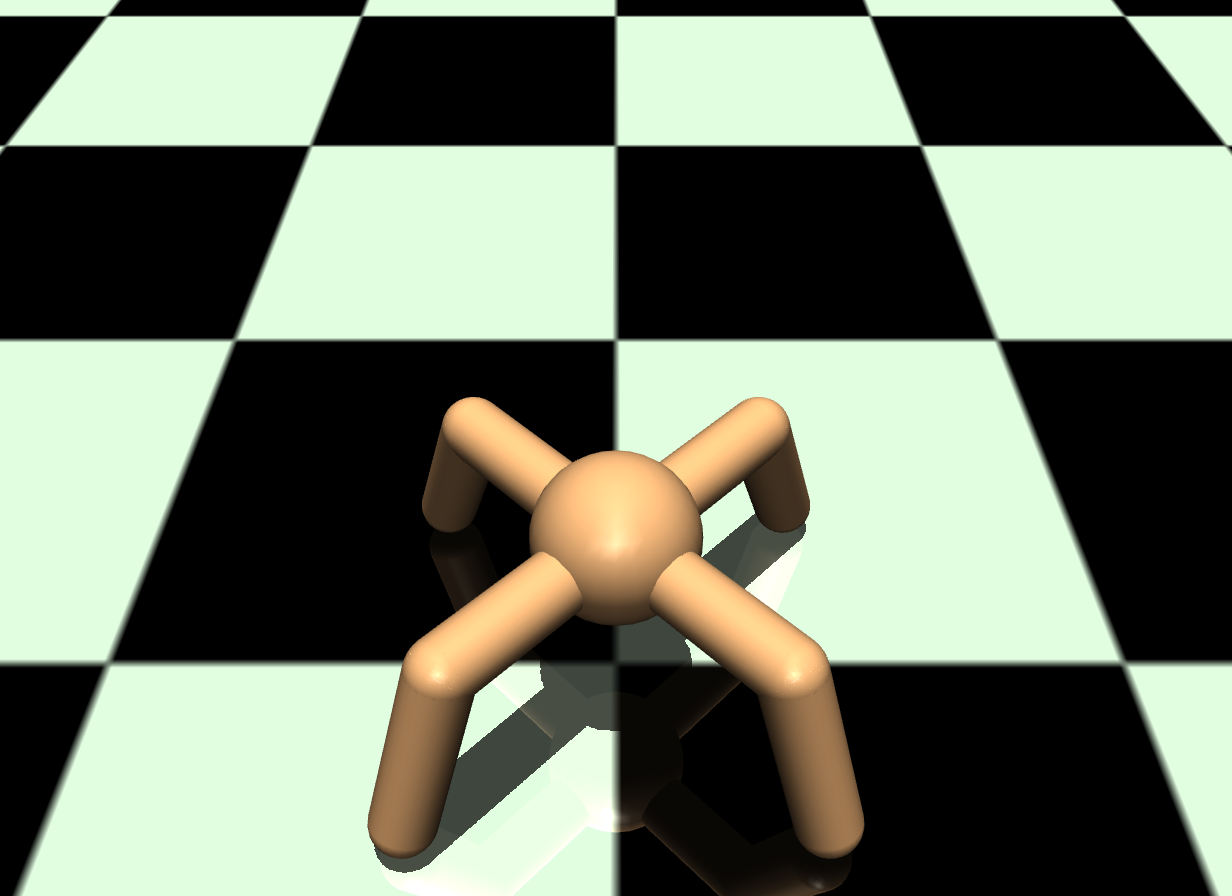
(b)

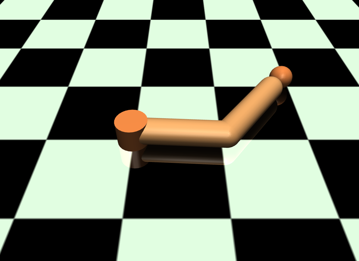
(c)

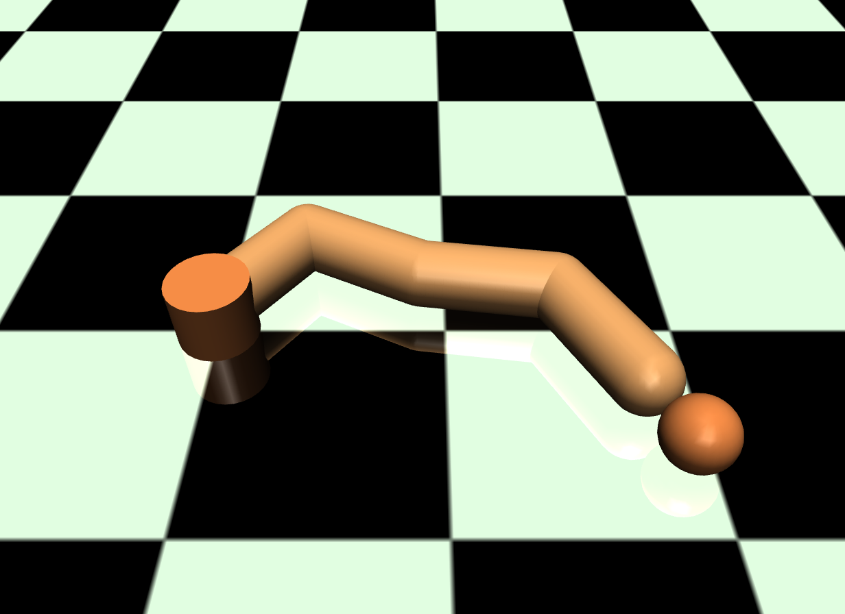
(d)

Figure 3: Renderings of the (3(a)) wheeled agent, (3(b)) quadrupedal ant, (3(c)) 2-link reacher, and (3(d)) 4-link reacher.

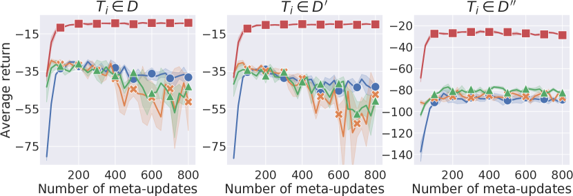
(a) Wheeled locomotion.

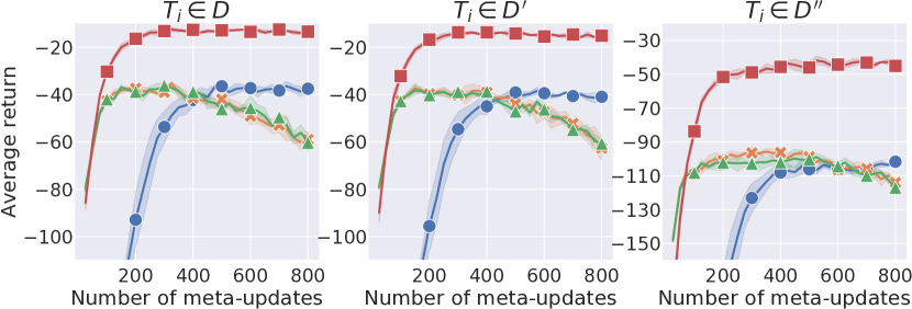
(b) Ant locomotion.

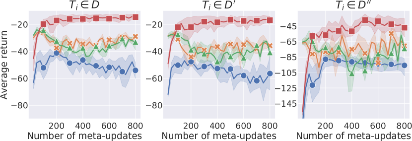
(c) 2-link reacher.

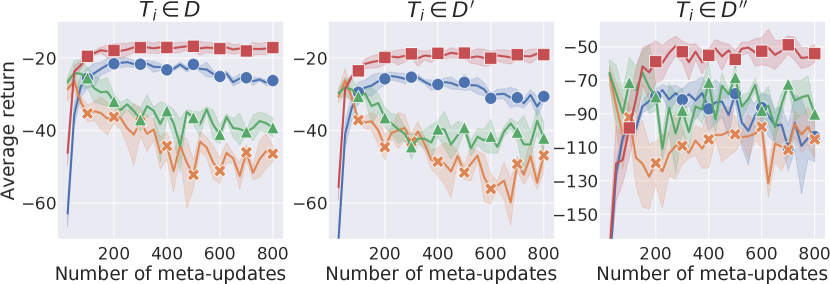
(d) 4-link reacher.

Figure 4: Learning curves on training and testing tasks. The y-axis represents the average return after $3$ fast-updates over all tasks. We directly apply the models trained on $D$ to perform evaluations, and thus testing tasks $D^{\prime}$ and $D^{\prime\prime}$ are not seen during the training of models. The plots are averaged over the best performing $3$ random seeds out of $10$ random seeds. For easy reading, the y-axes of some plots are truncated and the markers are plotted every $100$ meta-updates.

5.2 Empirical Results

To better reflect the learning ability on training tasks and the generalization ability on novel tasks, we plot learning curves of different methods on both training and novel tasks as shown in Figure 4. Specifically, we perform evaluations on $D$, $D^{\prime}$, and $D^{\prime\prime}$ every $25$ meta-updates. In each evaluation, we apply the models of different methods to perform $3$ fast-updates for each task, and report the average return after fast-updates over all tasks. The reported returns are calculated by $R=\frac{1}{100}\sum_{T_{i}}\sum_{t}r_{i,t}^{\text{dist}}$, where $100$ indicates the size of $D$, $D^{\prime}$, or $D^{\prime\prime}$, and $r_{i,t}^{\text{dist}}$ is the distance reward which is the negative distance to the target location.

From Figure 4, we observe that TESP significantly outperforms all baselines on $D$, which indicates TESP has better learning capacity than baselines on training tasks and is expected since TESP uses a more complex network (i.e., an extra RNN for the task encoder). In addition, all methods including our TESP and baselines have similar learning curves on $D$ and $D^{\prime}$, which demonstrates their ability to generalize to novel tasks sampled from the training distribution. However, the baselines tend to overfit to the training distribution and show poor performance on out-of-distribution tasks $D^{\prime\prime}$, but our TESP still has good performance on $D^{\prime\prime}$. Moreover, the gap between the performance of TESP on training and out-of-distribution tasks is smaller than those of baselines. Therefore, the reason why TESP shows better performance on $D^{\prime\prime}$ is not only that TESP learns training tasks better, but also that TESP is more generalizable.

The comparison with AdaptSV shows that simply adapting a single variable is not enough to represent different tasks. In contrast, our method is able to efficiently obtain a task embedding to represent each task by leveraging past experience stored in an episode buffer with a meta-learned task encoder. On the other hand, the convergence of TESP is more stable as the number of meta-updates increases, and the variance of TESP over different random seeds is smaller than baselines.

5.3 Ablation Studies

Since we introduce several different ideas into TESP, including the episode buffer holding the best $M$ experienced episodes for each task, the learnable SGD optimizer for task encoders, the shared policy, the regularization term in Eq. (10), and adaptive per-parameter learning rates of the learnable SGD optimizer, we perform ablations to investigate the contributions of these different ideas. Variants considered are (1) the episode buffer holding all experienced episodes for each task, (2) additionally fast-updating the policy for each task, (3) $\eta=0$ (i.e., without the regularization term), (4) $\alpha=0$ (i.e., without the SGD optimizer for fast-updating task encoders), and (5) holding constant the learning rate of the SGD optimizer. From Figure 5, we observe that most variants have similar performance to TESP on $D$ and $D^{\prime}$, but perform much worse on $D^{\prime\prime}$. The comparison with V1 shows that episodes with low rewards have a bad impact on the learning of task embeddings. Comparing TESP with V2 and V3, we confirm that the shared policy and the regularization term enable better generalization, especially for out-of-distribution novel tasks. The results of V4 indicate that it is crucial to leverage the proposed architecture in a meta-learning manner. As in prior works Li et al. (2017); Al-Shedivat et al. (2017); Gupta et al. (2018b), we also find that adaptive per-parameter learning rates can lead to better performance by comparing TESP with V5.

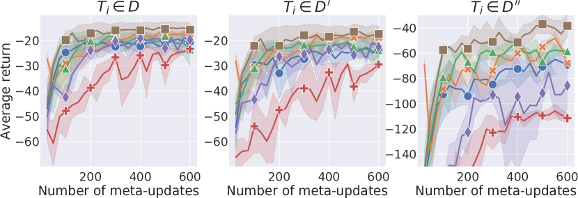
Figure 5: Ablation studies on 2-link reacher tasks.

6 Conclusion

In this work, we presented TESP, of which the basic idea is to explicitly model the individuality and commonness of tasks in the scope of meta-RL. Specifically, TESP trains a shared policy and an SGD optimizer coupled to a task encoder network from a set of tasks. When it comes to a novel task, we apply the SGD optimizer to quickly learn a task encoder which generates the corresponding task embedding, while the shared policy remains unchanged and just predicts actions based on observations and the task embedding. In future work, an interesting idea would be to extend TESP with a set of shared conditional policies inspired by Frans et al. (2018).

References

- Al-Shedivat et al. [2017] Maruan Al-Shedivat, Trapit Bansal, Yuri Burda, Ilya Sutskever, Igor Mordatch, and Pieter Abbeel. Continuous adaptation via meta-learning in nonstationary and competitive environments. arXiv preprint arXiv:1710.03641, 2017.
- Clavera et al. [2018] Ignasi Clavera, Anusha Nagabandi, Ronald S Fearing, Pieter Abbeel, Sergey Levine, and Chelsea Finn. Learning to adapt: Meta-learning for model-based control. arXiv preprint arXiv:1803.11347, 2018.
- Duan et al. [2016] Yan Duan, John Schulman, Xi Chen, Peter L Bartlett, Ilya Sutskever, and Pieter Abbeel. RL2: Fast reinforcement learning via slow reinforcement learning. arXiv preprint arXiv:1611.02779, 2016.
- Finn et al. [2017] Chelsea Finn, Pieter Abbeel, and Sergey Levine. Model-agnostic meta-learning for fast adaptation of deep networks. arXiv preprint arXiv:1703.03400, 2017.
- Florensa et al. [2017] Carlos Florensa, Yan Duan, and Pieter Abbeel. Stochastic neural networks for hierarchical reinforcement learning. In ICLR, 2017.
- Frans et al. [2018] Kevin Frans, Jonathan Ho, Xi Chen, Pieter Abbeel, and John Schulman. Meta learning shared hierarchies. In ICLR, 2018.
- Gupta et al. [2018a] Abhishek Gupta, Benjamin Eysenbach, Chelsea Finn, and Sergey Levine. Unsupervised meta-learning for reinforcement learning. arXiv preprint arXiv:1806.04640, 2018.
- Gupta et al. [2018b] Abhishek Gupta, Russell Mendonca, YuXuan Liu, Pieter Abbeel, and Sergey Levine. Meta-reinforcement learning of structured exploration strategies. In NIPS, 2018.
- Houthooft et al. [2018] Rein Houthooft, Richard Y Chen, Phillip Isola, Bradly C Stadie, Filip Wolski, Jonathan Ho, and Pieter Abbeel. Evolved policy gradients. arXiv preprint arXiv:1802.04821, 2018.
- Kang and Feng [2018] Bingyi Kang and Jiashi Feng. Transferable meta learning across domains. In UAI, 2018.
- Kingma and Welling [2013] Diederik P Kingma and Max Welling. Auto-encoding variational bayes. arXiv preprint arXiv:1312.6114, 2013.
- Levine et al. [2016] Sergey Levine, Chelsea Finn, Trevor Darrell, and Pieter Abbeel. End-to-end training of deep visuomotor policies. JMLR, 2016.
- Li et al. [2017] Zhenguo Li, Fengwei Zhou, Fei Chen, and Hang Li. Meta-sgd: Learning to learn quickly for few shot learning. arXiv preprint arXiv:1707.09835, 2017.
- Lillicrap et al. [2015] Timothy P Lillicrap, Jonathan J Hunt, Alexander Pritzel, Nicolas Heess, Tom Erez, Yuval Tassa, David Silver, and Daan Wierstra. Continuous control with deep reinforcement learning. arXiv preprint arXiv:1509.02971, 2015.
- Ma et al. [2018] Jiaqi Ma, Zhe Zhao, Xinyang Yi, Jilin Chen, Lichan Hong, and Ed H Chi. Modeling task relationships in multi-task learning with multi-gate mixture-of-experts. In SIGKDD, 2018.
- Mishra et al. [2017] Nikhil Mishra, Mostafa Rohaninejad, Xi Chen, and Pieter Abbeel. Meta-learning with temporal convolutions. arXiv preprint arXiv:1707.03141, 2017.
- Mnih et al. [2013] Volodymyr Mnih, Koray Kavukcuoglu, David Silver, Alex Graves, Ioannis Antonoglou, Daan Wierstra, and Martin Riedmiller. Playing atari with deep reinforcement learning. arXiv preprint arXiv:1312.5602, 2013.
- Ruder [2017] Sebastian Ruder. An overview of multi-task learning in deep neural networks. arXiv preprint arXiv:1706.05098, 2017.
- Schulman et al. [2017] John Schulman, Filip Wolski, Prafulla Dhariwal, Alec Radford, and Oleg Klimov. Proximal policy optimization algorithms. arXiv preprint arXiv:1707.06347, 2017.
- Silver et al. [2016] David Silver, Aja Huang, Chris J Maddison, Arthur Guez, Laurent Sifre, George Van Den Driessche, Julian Schrittwieser, Ioannis Antonoglou, Veda Panneershelvam, Marc Lanctot, et al. Mastering the game of go with deep neural networks and tree search. Nature, 2016.
- Snell et al. [2017] Jake Snell, Kevin Swersky, and Richard Zemel. Prototypical networks for few-shot learning. In NIPS, 2017.
- Stadie et al. [2018] Bradly C Stadie, Ge Yang, Rein Houthooft, Xi Chen, Yan Duan, Yuhuai Wu, Pieter Abbeel, and Ilya Sutskever. Some considerations on learning to explore via meta-reinforcement learning. arXiv preprint arXiv:1803.01118, 2018.
- Sutton et al. [1998] Richard S Sutton, Andrew G Barto, et al. Reinforcement learning: An introduction. MIT press, 1998.
- Tirinzoni et al. [2018] Andrea Tirinzoni, Rafael Rodriguez Sanchez, and Marcello Restelli. Transfer of value functions via variational methods. In NIPS, 2018.
- Todorov et al. [2012] Emanuel Todorov, Tom Erez, and Yuval Tassa. Mujoco: A physics engine for model-based control. In IROS, 2012.
- Williams [1992] Ronald J Williams. Simple statistical gradient-following algorithms for connectionist reinforcement learning. Machine Learning, 1992.
- Xu et al. [2018a] Kelvin Xu, Ellis Ratner, Anca Dragan, Sergey Levine, and Chelsea Finn. Learning a prior over intent via meta-inverse reinforcement learning. arXiv preprint arXiv:1805.12573, 2018.
- Xu et al. [2018b] Tianbing Xu, Qiang Liu, Liang Zhao, Wei Xu, and Jian Peng. Learning to explore with meta-policy gradient. arXiv preprint arXiv:1803.05044, 2018.
- Xu et al. [2018c] Zhongwen Xu, Hado van Hasselt, and David Silver. Meta-gradient reinforcement learning. arXiv preprint arXiv:1805.09801, 2018.