Axial Vector Form Factors from Lattice QCD that Satisfy the PCAC Relation

Abstract

Previous lattice QCD calculations of axial vector and pseudoscalar form factors show significant deviation from the partially conserved axial current (PCAC) relation between them. Since the original correlation functions satisfy PCAC, the observed deviations from the operator identity cast doubt on whether all the systematics in the extraction of form factors from the correlation functions are under control. We identify the problematic systematic as a missed excited state, whose energy as a function of the momentum transfer squared, $Q^{2}$, is determined from the analysis of the 3-point functions themselves. Its mass is much smaller than those of the excited states previously considered and including it impacts the extraction of all the ground state matrix elements. The form factors extracted using these mass/energy gaps satisfy PCAC and other consistency conditions, and validate the pion-pole dominance hypothesis. We also show that the extraction of the axial charge $g_{A}$ is very sensitive to the value of the mass gaps of the excited states used and current lattice data do not provide an unambigous determination of these, unlike the $Q^{2}\neq 0$ case. To highlight the differences and improvement between the conventional versus the new analysis strategy, we present a comparison of results obtained on a physical pion mass ensemble at $a\approx 0.0871$ fm. With the new strategy, we find $g_{A}=1.30(6)$. A very significant improvement over previous lattice results is found for the axial charge radius $r_{A}=0.74(6)$ fm, extracted using the $z$-expansion to parameterize the $Q^{2}$ behavior of $G_{A}(Q^{2})$, and $g_{P}^{\ast}=8.06(44)$ obtained using the pion pole-dominance ansatz to fit the $Q^{2}$ behavior of the induced pseudoscalar form factor $\widetilde{G}_{P}(Q^{2})$.

The nucleon axial form factor $G_{A}(Q^{2})$ is an important input needed to calculate the cross-section of neutrinos off nuclear targets. It is not well-determined experimentally Bernard et al. (2002), and the most direct measurements using liquid hydrogen targets are unlikely to be performed due to safety concerns. At present, these form factors are typically extracted from measurements of scattering off nuclear targets and involves modeling of nuclear effects Carlson et al. (2015); Aguilar-Arevalo et al. (2010), which introduces uncertainties Hill et al. (2018). Lattice QCD provides the best approach to calculate these from first principles, however, one has to demonstrate that all systematics are under control.

The axial, $G_{A}$, and the induced pseudoscalar, $\widetilde{G}_{P}$, form factors are extracted from the matrix elements of the four components of the isovector axial current $A_{\mu}\equiv\overline{u}\gamma_{5}\gamma_{\mu}d$ between the ground state of the nucleon:

$$\left\langle N({\bm{p}}_{f})|A_{\mu}(\vec{q})|N({\bm{p}}_{i})\right\rangle=\\ {\overline{u}}_{N}({\bm{p}}_{f})\left(G_{A}(q^{2})\gamma_{\mu}+q_{\mu}\frac{\tilde{G}_{P}(q^{2})}{2M}\right)\gamma_{5}u_{N}({\bm{p}}_{i}),$$ (1)

and the pseudoscalar form factor $G_{P}$ from

$$\left\langle N({\bm{p}}_{f})|P(\vec{q})|N({\bm{p}}_{i})\right\rangle={\overline{u}}_{N}({\bm{p}}_{f})G_{P}(q^{2})\gamma_{5}u_{N}({\bm{p}}_{i})\,,$$ (2)

where $P=\overline{u}\gamma_{5}d$ is the pseudoscalar density, $N({\bm{p}})$ is the nucleon state with mass $M$ and lattice momentum ${\bm{p}}\equiv 2\pi{\bm{n}}/La$ with ${\bm{n}}\equiv(n_{1},n_{2},n_{3})$. We neglect the induced tensor form factor $\tilde{G}_{T}$ in Eq. (1) since we assume isospin symmetry, $m_{u}=m_{d}$, throughout Bhattacharya et al. (2012). All the form factors will be presented as functions of the spacelike four-momentum transfer $Q^{2}\equiv{\bf p}^{2}-(E-M)^{2}=-q^{2}$.

In our previous work Gupta et al. (2017), we showed that form factors with good statistical precision can be obtained from lattice simulations, however, these data do not satisfy the partially conserved axial current (PCAC) relation:

$$2{\widehat{m}}G_{P}(Q^{2})=2MG_{A}(Q^{2})-\frac{Q^{2}}{2M}{\tilde{G}}_{P}(Q^{2})\,,$$ (3)

where ${\widehat{m}}$ is the PCAC quark mass. Such a failure has also been observed in all other lattice calculations Bali et al. (2015); Green et al. (2017); Alexandrou et al. (2017); Capitani et al. (2019); Ishikawa et al. (2018); Shintani et al. (2019). Since PCAC is an operator relation, it is important to find the systematic responsible for the deviation, and remove it prior to comparing lattice data with phenomenology.

In this work we show that the problematic systematic is a missed lower energy excited state. Using data from a physical pion mass ensemble, $a09m130W$ Jang et al. (2019a), we show how the mass and energy gap of this state can be determined from the analysis of nucleon 3-point correlation functions. We then demonstrate that form factors extracted including these parameters satisfy PCAC and other consistency conditions. With these improvements, we claim that the combined uncertainty in the lattice data is reduced to below ten percent level.

All lattice data presented here are from our calculations using the clover-on-HISQ formulation Gupta et al. (2017); Jang et al. (2019a). The gauge configurations are from the physical-mass $2+1+1$-flavor HISQ ensemble $a09m130W$ generated by the MILC collaboration Bazavov et al. (2013) with lattice spacing $a\approx 0.0871\,\mathrm{fm}$ and $M_{\pi}=130\,\mathrm{MeV}$. The pion mass on these configurations with the clover valence quark action is $M_{\pi}\approx 138\,\mathrm{MeV}$. Further details of the lattice parameters and methodology, statistics, the interpolating operator used to construct the 2- and 3-point correlation functions can be found in Refs. Jang et al. (2019a); Gupta et al. (2017).

The nucleon operator used to create and annihilate the nucleon state couples to the ground and all the excited and multiparticle states with appropriate quantum numbers. To isolate the ground state matrix elements, we fit the data for the 2- and 3-point functions, $C^{\text{2pt}}$ and $C_{\Gamma}^{\text{3pt}}$, using their spectral decompositions. For the 2-point functions, the four states truncation is

$$C^{\text{2pt}}(\tau,\bm{p})= {|{\cal A}_{0}|}^{2}e^{-E_{0}\tau}+{|{\cal A}_{1}|}^{2}e^{-E_{1}\tau}\,+$$

$${|{\cal A}_{2}|}^{2}e^{-E_{2}\tau}+{|{\cal A}_{3}|}^{2}e^{-E_{3}\tau}\,,$$ (4)

where ${\cal A}_{i}$ are the amplitudes and $E_{i}$ are the energies with momentum $\bm{p}$. The data and fits using Eq. (4) are shown in Fig. 1 (left). There is a reasonable plateau at large $\tau$ in $M_{\rm eff}(\tau)\equiv\log\frac{C^{\rm 2pt}(\tau)}{C^{\rm 2pt}(\tau+1)}$ for all momenta up to ${\bm{n}}^{2}=6$. The right panel shows $M_{\rm eff}$, $M_{0}$, and the first two mass gaps, determined using a variant of the Prony’s method Fleming et al. (2009), that are consistent with those obtained from 4-state fits Jang et al. (2019a).

The two-state truncation of the 3-point functions $C_{\Gamma}^{(3\text{pt})}(t;\tau;\bm{p}^{\prime},\bm{p})$, with Dirac index $\Gamma$, is

$$C_{\Gamma}^{3\text{pt}} (t;\tau;\bm{p}^{\prime},\bm{p})=$$

$$\lvert\mathcal{A}_{0}^{\prime}\rvert\lvert\mathcal{A}_{0}\rvert\langle 0^{\prime}\lvert\mathcal{O}_{\Gamma}\rvert 0\rangle e^{-E_{0}t-M_{0}(\tau-t)}+$$

$$\lvert\mathcal{A}_{0}^{\prime}\rvert\lvert\mathcal{A}_{1}\rvert\langle 0^{\prime}\lvert\mathcal{O}_{\Gamma}\rvert 1\rangle e^{-E_{0}t-M_{1}(\tau-t)}+$$

$$\lvert\mathcal{A}_{1}^{\prime}\rvert\lvert\mathcal{A}_{0}\rvert\langle 1^{\prime}\lvert\mathcal{O}_{\Gamma}\rvert 0\rangle e^{-E_{1}t-M_{0}(\tau-t)}+$$

$$\lvert\mathcal{A}_{1}^{\prime}\rvert\lvert\mathcal{A}_{1}\rvert\langle 1^{\prime}\lvert\mathcal{O}_{\Gamma}\rvert 1\rangle e^{-E_{1}t-M_{1}(\tau-t)}\,,$$ (5)

where the source point is translated to $t=0$, the operator is inserted at time $t$, and the nucleon is annihilated at the sink time slice $\tau$. In this relation, $|0\rangle$ and $|n\rangle$ are the ground and $n^{\rm th}$ excited state. The superscript ^′ denotes that the state could have nonzero momentum $\bm{p}^{\prime}$. The momentum transfer $\bm{q}=\bm{p}^{\prime}-\bm{p}=\bm{p}^{\prime}$ since $\bm{p}$ at the sink is fixed to zero. The $M_{i}$, $E_{i}$ and ${\cal A}_{i}^{\prime}|A_{i}$ are the masses, energies and the amplitudes for the creation$|$annihilation of these states by the nucleon interpolating operator.

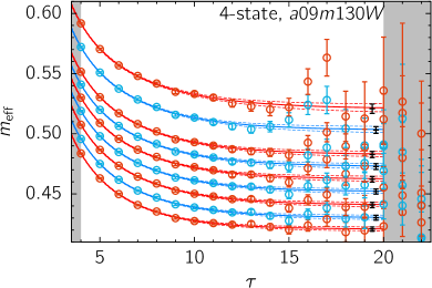
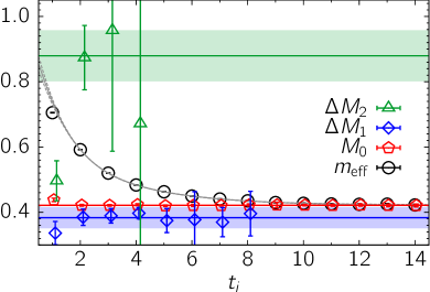
Figure 1: The left panel shows the effective energy $E_{\rm eff}(\tau)=\log\frac{C^{\rm 2pt}(\tau)}{C^{\rm 2pt}(\tau+1)}$ and the 4-state fit for various momentum channels. The right panel compares the nucleon $M_{\rm eff}$ at $\bm{p}=0$ with $M_{0}$ (red band), the first mass gap $\Delta M_{1}\equiv M_{1}-M_{0}$ (blue band), and the second mass gap $\Delta M_{2}\equiv M_{2}-M_{0}$ (green band). These are obtained using the Prony’s method with fits to the intervals $[t_{i},t_{i}+6]$, where $t_{i}$ is the starting time slice. Sensitivity to $\Delta M_{1}$ ($\Delta M_{2}$) is lost at $t_{i}=8$ ($t_{i}=4$). All data are in lattice units.

To display and discuss the data, it is much more convenient and common to consider the five ratios, ${\cal R}_{5\mu}$ and ${\cal R}_{5}$, of the 3-point correlation functions of $A_{\mu}$ and $P$ to the 2-point correlator as defined in Ref. Gupta et al. (2017):

$${\cal R}_{51}\rightarrow \;\frac{1}{\sqrt{(2E_{p}(E_{p}+M))}}\left[-\frac{q_{1}q_{3}}{2M}{\tilde{G}}_{P}\right]\,,$$ (6)

$${\cal R}_{52}\rightarrow \;\frac{1}{\sqrt{(2E_{p}(E_{p}+M))}}\left[-\frac{q_{2}q_{3}}{2M}{\tilde{G}}_{P}\right]\,,$$ (7)

$${\cal R}_{53}\rightarrow \;\frac{1}{\sqrt{(2E_{p}(E_{p}+M))}}\left[-\frac{q_{3}^{2}}{2M}{\tilde{G}}_{P}+(M+E_{p})G_{A}\right]\,,$$ (8)

$${\cal R}_{54}\rightarrow \;\frac{4Mq_{3}}{\sqrt{(2E_{p}(E_{p}+M))}}\left[\frac{M-E_{p}}{2M}G_{P}+G_{A}\right]\,,$$ (9)

$${\cal R}_{5}\rightarrow \;\frac{1}{\sqrt{(2E_{p}(E_{p}+M))}}\left[q_{3}{G}_{P}\right]\,.$$ (10)

where $q_{i}$ is the momentum transferred by the current in the “i” spatial direction. The direction “3” is singled out since it is chosen to be the direction of the spin projection of the Dirac spinors in the construction of the 3-point functions. In the limit of large source-sink separation, $\tau\to\infty$, these ratios give the combination of the form factors shown on the right hand side. We have explicitly displayed the kinematic factors to show which momentum combinations have a signal in each case. Data with equivalent momenta are averaged in the analysis.

Equations (6)–(9) form an over-complete set. ${\cal R}_{51}$ and ${\cal R}_{52}$ can be averaged as they are related by the lattice cubic symmetry and give $\widetilde{G}_{P}$. For $q_{3}=0$, ${\cal R}_{53}$ gives $G_{A}$. For the other momentum combinations, one gets a linear combination of $G_{A}$ and $\widetilde{G}_{P}$. Thus, the three $A_{i}$ correlators give results for $G_{A}$ and ${\tilde{G}}_{P}$ for all values of momentum transfer. Consequently, data from $A_{4}$ correlators have traditionally Bali et al. (2015); Gupta et al. (2017); Green et al. (2017); Alexandrou et al. (2017); Capitani et al. (2019); Ishikawa et al. (2018); Shintani et al. (2019) been neglected because they exhibits very large excited-state contamination (ESC) as shown in Fig. 2. Lastly, $G_{P}$ is obtained uniquely from Eq. (10).

In our previous work Gupta et al. (2017), the energies of the excited state used to isolate the ground state matrix elements in fits to the 3-point functions were taken from four-state fits to the 2-point correlation function defined in Eq. (4). The resulting form factors violated PCAC. Furthermore, the violation increased as $Q^{2}\to 0$, $a\to 0$ and $M_{\pi}\to M_{\pi}^{\rm physical}$. Correcting for $O(a)$ lattice artifacts in the axial current showed no significant reduction in the violation Gupta et al. (2017).

In this paper we show that by using these values of $M_{i}$ and $E_{i}$ to remove the ESC we missed a lower excited state. Furthermore, the energy of this state can be determined from the analysis of the $A_{4}$ correlator, ie, the channel with the largest ESC is the most sensitive to it.

In Fig. 2, we compare the conventional 3^∗-state fit to the $A_{4}$ correlator with masses and energies, $M_{i}$ and $E_{i}$, taken from the 4-state fit to the 2-point function Gupta et al. (2017) versus the new two-state fit with $M_{1}$ and $E_{1}$ left as free parameters. The $\chi^{2}/{\rm DOF}$ and $p$-value of the fits for all ten momentum cases are given in Table 1. Note that for ${\bm{n}}=(0,0,1)$, $\chi^{2}/{\rm DOF}$ reduces from 21.8 to 0.8. The values of the mass$|$energy gaps of the “first” excited state shown in Fig. 3 are much smaller, and close to those expected for non-interacting $N({\bm{p}})\pi(-{\bm{p}})$ and $N(0)\pi({\bm{p}})$ states Bar (2019). By ${\bm{n}}^{2}\gtrsim 6$, the mass gaps become similar and, correspondingly, the violation of PCAC at larger momentum-transfer are observed to be small (see Fig. 6 and Ref. Gupta et al. (2017)). We hypothesize that this lower energy excited state provides the dominant contamination in all five 3-point correlation functions. On the basis of consistency checks including PCAC, we make the case that it is essential to include this lower energy excited state in all the fits used to remove the ESC.

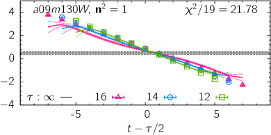
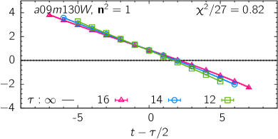
Figure 2: Comparison of the fits used to remove ESC in the $A_{4}$ 3-point function using the ${\cal S}_{\rm 2pt}$ (left) and ${\cal S}_{\rm A4}$ (right) strategies defined in the text. This data for ${\bm{p}}=(1,0,0)2\pi/La$ show the largest ESC. The values of $\tau$ and $\chi^{2}$/DOF are given in the legend.

Table 1: The goodness of the fits to $C^{\rm 3pt}_{A_{4}}$. The new 2-state fits correspond to strategy ${\cal S}_{\rm A4}$ defined in the text. The conventional 3^∗-state fit values (strategy ${\cal S}_{\rm 2pt}$) are taken from Refs. Jang et al. (2018); Gupta et al. (2018).

	New 2-state		Conventional 3∗-state
$\bm{n}^{2}$	$\chi^{2}/\text{d.o.f}$	$p$	$\chi^{2}/\text{d.o.f}$	$p$
1	0.817	0.73	21.78	$<5\times 10^{-5}$
2	1.314	0.13	19.36	$<5\times 10^{-5}$
3	1.263	0.16	11.79	$<5\times 10^{-5}$
4	0.778	0.79	4.757	$<5\times 10^{-5}$
5	1.268	0.16	5.348	$<5\times 10^{-5}$
6	1.712	0.01	4.834	$<5\times 10^{-5}$
8	0.815	0.74	1.724	0.03
9  (2,2,1)	1.865	0.01	2.726	0.001
9′ (3,0,0)	0.539	0.98	0.974	0.49
10	0.865	0.67	1.089	0.35

To highlight the differences and improvements, we define two analysis strategies, “conventional”, ${\cal S}_{\rm 2pt}$, and “new”, ${\cal S}_{\rm A4}$:

• ${\cal S}_{\rm 2pt}$: All the ground and excited state $M_{i}$ and $E_{i}$, are taken from 4-state fits to the nucleon 2-point function and used in the $3^{\ast}$-state analysis of all the 3-point functions as detailed in Ref. Jang et al. (2019a).

• ${\cal S}_{\rm A4}$: The ground state parameters $M_{0}$ and $E_{0}$ are taken from the 4-state fits to the nucleon 2-point function. These are considered reliable based on the observed plateau in the effective-mass data at large $\tau$ as shown in Fig. 1. The parameters for the first excited state, $M_{1}$ and $E_{1}$, are taken from fits to the $A_{4}$ 3-point correlator as discussed above. These are then used in a two-state analysis of all other 3-point functions.

In both cases, it is important to note that residual ESC may still be present in the $M_{i}$ and $E_{i}$. Future higher precision calculations will improve the precision of the calculations by steadily including more states in the fits.

In Fig. 3, we show three sets of data for the energy gaps of the first excited state: $\Delta E_{1}^{\rm 2pt}\equiv E_{1}^{\rm 2pt}-E_{0}$ obtained from fits to the 2-point correlator. These are compared with the two values on either side of the $A_{4}$ operator insertion, which are expected to be different since the correlator is projected to zero-momentum at the sink: $\Delta M_{1}^{A_{4}}\equiv M_{1}^{A_{4}}-M_{0}$, the zero momentum case on the sink side and the non-zero-momentum values $\Delta E_{1}^{A_{4}}\equiv E_{1}^{A_{4}}-E_{0}$ on the source side. It is clear that $\Delta E_{1}^{A_{4}}$ and $\Delta M_{1}^{A_{4}}$ are much smaller than $\Delta E_{1}^{\rm 2pt}$ for ${\bm{n}}^{2}\lesssim 6$ indicating the contribution of a lower energy excited state. Secondly, $\Delta E_{1}^{A_{4}}$ and $\Delta M_{1}^{A_{4}}$ are significantly different. Strategy ${\cal S}_{\rm 2pt}$ corresponds to using $\Delta E_{1}^{\rm 2pt}$ and $\Delta M_{1}^{\rm 2pt}$, whereas ${\cal S}_{\rm A4}$ corresponds to using $\Delta E_{1}^{A_{4}}$ and $\Delta M_{1}^{A_{4}}$.

In Fig. 3, we also show, using dotted lines, the expected values for $\Delta E$ and $\Delta M$ if we assume that the leading contribution of the current $A_{4}(\bm{q})$ is to insert or remove a pion with momentum $\bm{q}$. Thus the plotted $\Delta E$ corresponds to the values for a non-interacting state $N({\bm{p}}=0)\pi({\bm{p}})$, while $\Delta M_{1}$ to $N({\bm{p}})\pi(-{\bm{p}})$. In calculating these values, we have used the lattice values for $M_{0}$ and $M_{\pi}$ and the relativistic dispersion relation, which is consistent with the data from the 2-point function. The values and variation of $\Delta E_{1}^{A_{4}}$ and $\Delta M_{1}^{A_{4}}$ with ${\bm{n}}^{2}$ are roughly consistent with this picture.

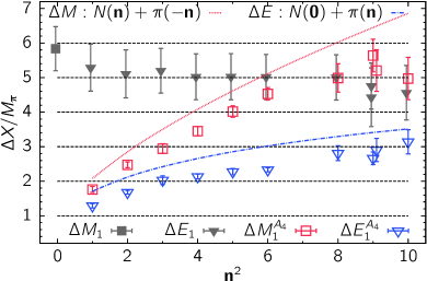
Figure 3: Mass and energy gaps $\Delta M_{1}=M_{1}-M_{0}$ and $\Delta E_{1}(\bm{n}^{2})=E_{1}^{\text{2pt}}-E_{0}$ in units of $M_{\pi}$ are obtained from the 4-state fit to the 2-point correlator. The values $\Delta M_{1}^{A_{4}}$ and $\Delta E_{1}^{A_{4}}$ for the $a09m130W$ ensemble are obtained using strategy ${\cal S}_{\rm A4}$. The dotted lines show the corresponding values for non-interacting $N({\bm{p}})\pi({\bm{-}p})$ and $N(0)\pi({\bm{p}})$ states.

Using the excited-state parameters extracted from the analysis of the $A_{4}$ correlator, and following the strategy ${\cal S}_{\rm A4}$ gives very different values for the ground state matrix elements extracted from the three spatial, $A_{i}$, and the $P$ correlators. A comparison of the 2-state fits using ${\cal S}_{\rm A4}$ and the $3^{\ast}$-state fit using ${\cal S}_{\rm 2pt}$ is shown in Fig. 4 for the lowest non-zero momentum channels. Based on the $\chi^{2}/$DOF of the fits, we cannot distinguish between the two strategies except for the $P$ channel in spite of having high statistics data (165K measurements on 1290 configurations) Jang et al. (2019a). The key point in each of the four channels is the convergence–it is from below and including the “new” lower excited state (${\cal S}_{\rm A4}$) gives significantly larger values of the matrix elements and thus the form factors. This pattern persists for ${\bm{n}}^{2}\lesssim 5$, above which the difference in the mass gap does not have a significant effect.

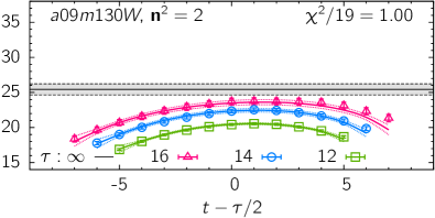
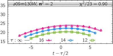
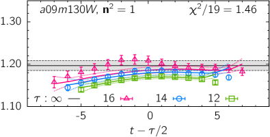
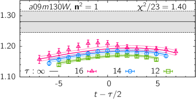
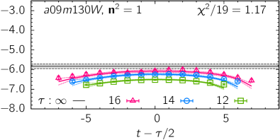
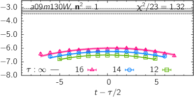
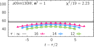
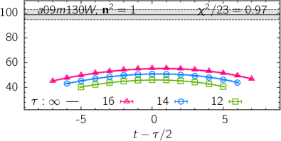
Figure 4: Comparison of the ground state matrix element (the horizontal grey band) obtained using the two strategies ${\cal S}_{\rm 2pt}$ (left panels) and ${\cal S}_{\rm A4}$ (right panels). In both cases, a 2-state fit is performed to the 3-point correlator. The four sets of figures are for: $A_{1}$ with ${\bm{n}}=(1,1,0)$ (top); $A_{3}$ with $q_{3}=0$ and ${\bm{n}}=(1,0,0)$ (second row); $A_{3}$ with ${\bm{n}}=(0,0,1)$ (third row); and $P$ with ${\bm{n}}=(1,0,0)$ (bottom row). The $\chi^{2}/$DOF and the values of $\tau$ used in the fit are shown in the legend.

The results for the three form factors $G_{A}$, $\widetilde{G}_{P}$ and $G_{P}$ are compared in Fig. 5. The effect of using ${\cal S}_{\rm A4}$ is clear and largest for ${\bm{n}}=(1,0,0)$. Also, the change in $G_{A}(Q^{2})$ is only apparent for ${\bm{n}}=(1,0,0)$, consequently data at smaller $Q^{2}$ are needed to quantify its $Q^{2}\to 0$ limit.

The pattern, that the effect increases as $Q^{2}\to 0$, $a\to 0$ and $M_{\pi}\to M_{\pi}^{\rm physical}$, is confirmed by the analysis of the 11 ensembles described in Ref. Jang et al. (2019a), and these detailed results will be presented in a separate longer paper Jang et al. (2019b).

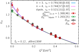
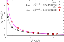
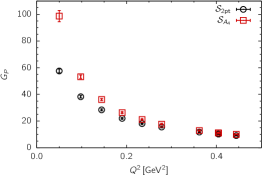
Figure 5: Comparison of $G_{A}$ (left), $(\widetilde{G}_{P})$ (middle) and $G_{P}$ (right) versus $Q^{2}$, in units of GeV², obtained using the two stategies ${\cal S}_{\rm A4}$ (red) and ${\cal S}_{\rm 2pt}$ (black). The lines show the dipole and $k^{3}$ and $k^{4}$ $z$-expansion fits to $G_{A}$ and PPD ansatz to $\widetilde{G}_{P}$.

With $G_{A}$, $\widetilde{G}_{P}$ and $G_{P}$ in hand, we present the test of the PCAC relation, Eq. (3), in Fig. 6. The figure also shows data for the pion-pole dominance (PPD) hypothesis that relates $\widetilde{G}_{P}$ to $G_{A}$ as ${\tilde{G}}_{P}(Q^{2})={G}_{A}(Q^{2})\frac{4M^{2}}{Q^{2}+M_{\pi}^{2}}$. It is clear that both relations are satisfied to within 5% at all $Q^{2}$ with ${\cal S}_{\rm A4}$, whereas the deviation grows to about 40% with ${\cal S}_{\rm 2pt}$ at ${\bm{n}}=(1,0,0)$ as first pointed out in Ref. Gupta et al. (2017). What is also remarkable is that the PPD relation with the expected proportionality factor $4M^{2}$ provided by the Goldberger-Treiman relation Goldberger and Treiman (1958) tracks the improvement in PCAC. In fact, the data for the two tests overlap at all $Q^{2}$.

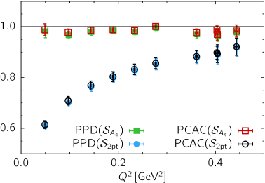
Figure 6: Comparison of the tests of the PCAC and the pion-pole dominance (PPD) hypothesis using the two analysis strategies ${\cal S}_{\rm A4}$ and ${\cal S}_{\rm 2pt}$ defined in the text. We plot the quantity $\frac{2{\widehat{m}}}{2M}\frac{G_{P}(Q^{2})}{G_{A}(Q^{2})}+\frac{Q^{2}}{4M^{2}}\frac{{\tilde{G}}_{P}(Q^{2})}{G_{A}(Q^{2})}$ for PCAC (open symbols) and $\frac{Q^{2}+M_{\pi}^{2}}{4M^{2}}\frac{{\tilde{G}}_{P}(Q^{2})}{G_{A}(Q^{2})}$ (filled symbols) for PPD. These should both be unity up to $O(a)$ corrections at all $Q^{2}$ if these relations hold.

The last test we perform is the relation $\partial_{4}A_{4}=(M-E)A_{4}$ that should be satisfied by the ground state matrix element. The data and fits for $\partial_{4}A_{4}$ are shown in Fig. 7. The values of $(M-E)A_{4}$ are essentially zero in both cases; for ${\cal S}_{\rm 2pt}$ because $M-E$ is small. Again, it is clear that the relation is only satisfied for ${\cal S}_{\rm A4}$.

The bottom line is that the two relations, PCAC and $\partial_{4}A_{4}=(M-E)A_{4}$, and the pion-pole dominance hypothesis are all satisfied using ${\cal S}_{\rm A4}$ but not with ${\cal S}_{\rm 2pt}$. The data shown in Fig. 3 is consistent with the picture that the “new” lower energy state is mainly due to the current $A_{\mu}(\bm{q})$ injecting a pion with momentum $\bm{q}$. There are two open questions: (i) how do we extract $g_{A}$, ie, what is the analogous lowest excited state at zero momentum since we cannot determine its parameters from the $A_{4}$ correlator, and (ii) why it was not clear from the data shown in Figs. 2 and 4 that the mass gaps used in ${\cal S}_{\rm 2pt}$ were too large. These points are addressed below.

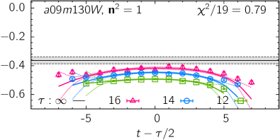
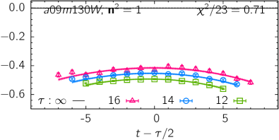
Figure 7: Data and fits to $\partial_{4}A_{4}$ using ${\cal S}_{\rm 2pt}$ (left) and ${\cal S}_{\rm A4}$ (right). The values of $\tau$ used and the $\chi^{2}/$DOF of the fits are given in the legend. The horizontal grey band showing the ground state value has tiny uncertainty in the right panel.

Results for $g_{A}$ have been obtained from the $A_{3}$ correlator at zero-momentum in all previous calculations because it has the best signal. The states with the lowest energy that are candidates for the $\frac{1}{2}({\frac{1}{2}}^{+})$ excited state at zero momentum in this correlator are $N\pi\pi$ and $N({\bm{p}})\pi({\bm{-}p})$. Both of these are lighter than the radial excitations N(1440) and N(1710) and dominate their decay. Their relativistic non-interacting energies, in a box of size $L/a=64$ used for the $a09m130W$ ensemble, are about 1230 MeV ($\Delta M_{1}a\approx 0.12$). Our previous argument favors $N\pi\pi$: the current $A_{3}({\bm{p}}=0)$ is more likely to insert a $\pi\pi$ state at zero momentum, whereas in the other case it would need to insert a pion with $({\bm{p}}=(1,0,0))$ and at the same time cause the transition $N(0)\to N({\bm{p}}=(-1,0,0))$ to ensure zero total momentum. In any case, since the only quantity that enters in our analysis is the mass gap and not the specifics of the excited state, we take the common value, $\Delta M=1230$ MeV, in the reanalysis of $A_{3}$ to extract $g_{A}$.

Table 2: Final results from both strategies, ${\cal S}_{\rm A4}$ and ${\cal S}_{\rm 2pt}$. $g_{A}$ is obtained in three ways as discussed in the text, and $r_{A}$ and $g_{P}^{\ast}$ from $z^{4}$ fits. Note these estimates are at fixed $a\approx 0.0871$ fm.

	$g_{A}|_{3pt}$	$g_{A}|_{z{\rm-exp}}$	$g_{A}|_{\rm dip}$	$r_{A}$(fm)	$g_{P}^{\ast}$
${\cal S}_{\rm A4}$	1.30(6)	1.30(7)	1.20(6)	0.74(6)	8.06(44)
${\cal S}_{\rm 2pt}$	1.25(2)	1.19(5)	1.20(5)	0.45(7)	4.67(24)

In what follows, all results for the renormalized axial current are presented using $Z_{A}=0.95(4)$ taken from Ref. Gupta et al. (2018). Fits to the zero-momentum $A_{3}$ correlator with prior $\Delta Ma=0.12(4)$ give $g_{A}$ in the range 1.29–1.31 depending on the values of $\tau$ used in the fit compared to $g_{A}=1.25(2)$ using ${\cal S}_{\rm 2pt}$ given in Ref. Gupta et al. (2018) (column 2 in Table 2). However, fits with priors in the range $0.1\lesssim\Delta M_{1}\lesssim 0.4$ are not distinguished on the basis of $\chi^{2}$/DOF. The output $\Delta M_{1}$ tracks the input prior, and the value of $g_{A}$ increases as the prior value is decreased. Thus, we regard this method as giving $g_{A}$ with uncontrolled systematics–the relevant $\Delta M_{1}$ has to be determined first. Parenthetically, similar fits to extract the scalar and tensor charges $g_{S}$ and $g_{T}$ are much more stable, the value of the output $\Delta M_{1}$ is far less senstitive to the prior and the results vary by $\lesssim 2\sigma$ as will be shown in Ref. Jang et al. (2019b).

Our current best estimate for $\Delta M_{1}$ on a given ensemble is to take the lower of the $N\pi\pi$ or $N({\bm{n}}^{1}=1)\pi({\bm{n}}^{2}=1)$ states. Assuming they are roughly degenerate, one can use the value of $\Delta M_{1}^{A4}a\approx 0.1$ shown in Fig. 3 at ${\bm{n}}^{2}=1$ that, as we have argued above, corresponds to the latter state. Using this $\Delta M_{1}^{A4}a$, our analysis of the $A_{3}$ data gives $g_{A}=1.30(6)$.

The second way we extract $g_{A}$ is to parameterize the $Q^{2}$ dependence of $G_{A}(Q^{2})$ using the $z$-expansion and the dipole ansatz. The $z$-expansion fits using the process defined in Ref. Gupta et al. (2017); Jang et al. (2019a) give $g_{A}=1.30(7)$ for ${\cal S}_{\rm A4}$ compared to $g_{A}=1.19(5)$ using ${\cal S}_{\rm 2pt}$. These results are independent of $k$ for $k>2$ in the $z^{k}$-expansion. The dipole fit gives $g_{A}=1.20(6)$ with a large $\chi^{2}$/DOF = 1.97 and the results are essentially the same for ${\cal S}_{\rm A4}$ and ${\cal S}_{\rm 2pt}$ as can be seen in Fig 5. One can fix the dipole fit to not miss the crucial low $Q^{2}$ points by putting a cut on $Q^{2}$, however, for this study we choose to neglect it.

The root-mean-squared charge radius extracted using the $z$-expansion fits gives $r_{A}=0.74(6)$ fm with ${\cal S}_{\rm A4}$ and $r_{A}=0.45(7)$ fm with ${\cal S}_{\rm 2pt}$. Once the lattice data have been extrapolated to the continuum limit, they can be compared with (i) a weighted world average of (quasi)elastic neutrino and antineutrino scattering data Bernard et al. (2002), (ii) charged pion electroproduction experiments Bernard et al. (2002), and (iii) a reanalysis of the deuterium target data Meyer et al. (2016):

$$r_{A} = 0.666(17)~{}{\rm fm}\qquad\nu,{\overline{\nu}}-{\rm scattering}\,,$$

$$r_{A} = 0.639(10)~{}{\rm fm}\qquad{\rm Electroproduction}\,,$$

$$r_{A} = 0.68(16)~{}{\rm fm}\,\ \qquad{\rm Deuterium}\,,$$ (11)

The induced pseudoscalar charge $g_{P}^{\ast}$, defined as

$$g_{P}^{\ast}\equiv\frac{m_{\mu}}{2M}{\tilde{G}}_{P}(Q^{2}=0.88m_{\mu}^{2})\,,$$ (12)

is obtained by fitting ${\tilde{G}}_{P}(Q^{2})$ using the small $Q^{2}$ expansion of the PPD ansatz:

$$\frac{m_{\mu}}{2M}\frac{{\tilde{G}}_{P}(Q^{2})}{g_{A}}=\frac{c_{1}}{M_{\pi}^{2}+Q^{2}}+c_{2}+c_{3}Q^{2}\,,$$ (13)

Our result using ${\cal S}_{\rm A4}$ is $g_{P}^{\ast}=8.06(44)$, while the MuCap experiment gave $g_{P}^{\ast}|_{\rm MuCap}=8.06(55)$ Andreev et al. (2013, 2015).

We caution the reader that all the results summarized in Table 2 are at fixed $a\approx 0.0871$ fm. Comparison to the phenomenological values should be made only after extrapolation to the continuum limit. The goal of this paper is to highlight the changes on using ${\cal S}_{\rm A4}$.

Second, we comment on why the lower-energy state is missed when following ${\cal S}_{\rm 2pt}$. It is well known that extracting $E_{i}$ from n-state fits to ${C}^{\rm 2pt}$ gives $E_{i}$ with ESC since the number of pre-plateau data point that are sensitive to excited states are typically 8–12 as shown in Fig. 1. While we find an $\approx 15\%$ change between a 2- and 4-state fit, we did not anticipate $E_{1}^{\rm A4}\sim E_{1}^{\rm 2pt}/4$ at small $Q^{2}$ as shown in Fig. 8. The known methodology to getting a more realistic excited state spectrum in a finite box with nucleon quantum numbers is to construct a large basis of interpolating operators, including operators overlapping primarily with multiparticle states, and solve the generalized eigenvalue problem (GEVP) Fox et al. (1982) in a variational approach Edwards et al. (2011); Alexandrou et al. (2014); Lang and Verduci (2014); Dudek (2018); Briceno et al. (2018). One should then compare the energies with lattice data, for example in the axial case with $E_{1}^{\rm A4}$, to determine which states contribute to a given 3-point function. This option will be explored in future calculations.

To get a rough picture of the impact of the choice of $E_{1}$ on the ESC in 3-point functions, assume that the prefactors in the two $0\leftrightarrow 1$ transition terms are equal and unity, and the $1\leftrightarrow 1$ term can be neglected in Eq. 5. Then the ESC should fall off exponentially as $e^{-(M_{1}-M_{0})(\tau/2)}+e^{-(E_{1}-E_{0})(\tau/2)}$. In Fig. 8, we plot this function for three typical values of $(M_{1}-M_{0})$ and $(E_{1}-E_{0})$ with ${\bm{n}}=(0,0,1)$. These values are from the 2- and 4-state fits to the 2-point function and those extracted from a 2-state fit to the $A_{4}$ 3-point function. Over the interval $10<\tau/a<16$, corresponding to 0.9–1.4 fm in which lattice data are typically collected, the exponential fall-off is approximately linear. Furthermore, the three curves in this range can be roughly aligned by a constant shift in their magnitude, ie, by just a change in the prefactors we have set to unity in Eq. 5, and which are free parameters in the actual fits. Thus, over a limited range of $\tau$, the expected exponential convergence can be masked to look linear. On the other hand, the size of the ESC is very sensitive to $E_{1}$ and large even at $\tau/a=25$ for $E_{1}^{A_{4}}$. The lesson is that while the excited state energy gaps impact the magnitude of the ESC at any given $\tau$, checks on the $E_{i}$ using 2-state fits and the convergence to $\tau\to\infty$ of ground state matrix elements is hard to judge from a limited range of $\tau$ even for very different energy gaps. As discussed above, the extraction of $g_{A}$ is plagued by this problem since we are not able to extract $M_{1}^{\rm A4}$ from a 3-point function. In short, it is very important to determine $E_{1}$ reliably. Once this is done, even 2-state fits give reasonable estimates of the $\tau\to\infty$ value based on the consistency checks discussed above.

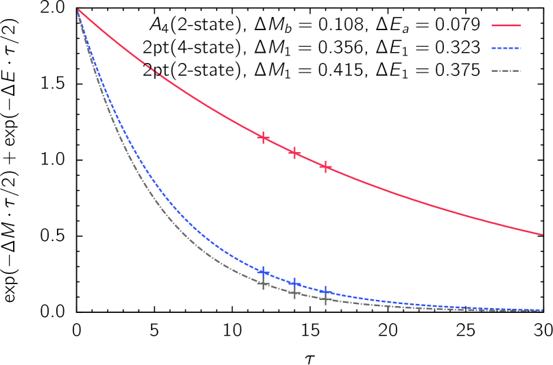
Figure 8: Cartoon of the behavior of the ESC in 3-point functions evaluated at the midpoint $t=\tau/2$ for three typical values of $(M_{1}-M_{0})$ and $(E_{1}^{{\bm{p}}}-E_{0}^{{\bm{p}}})$ as a function of the source-sink separation $\tau$. The plus symbols show the three values of $\tau/a=12,14,16$ at which the lattice data are presented.

An attempt to resolve the PCAC conundrum has been presented in Bali et al. (2019). We contend that it missed resolving the lower energy state and did not solve the problem. The projected currents $A_{\mu}^{\perp}$ and $P^{\perp}$ introduced in their work consist of a rotation in the basis of the five currents $A_{\mu}$ and $P$. For the lattice ensembles and parameters explored in their Bali et al. (2019) and our Gupta et al. (2017); Jang et al. (2019a) calculations, the three $A_{i}^{\perp}$ essentially remain within the space of the $A_{i}$. Thus, the ${\cal S}_{\rm 2pt}$ strategy with $A_{i}^{\perp}$ gives $G_{A}(Q^{2})$ and $\widetilde{G}_{P}$ that are essentially unchanged, and one continues to get a low value for $g_{P}^{\ast}$ Bali et al. (2019). The operator $A_{4}^{\perp}$ is mostly rotated into the $A_{i}$. Thus $A_{4}^{\perp}$ no longer shows the large ESC, and the “sinh” behavior illustrated in Fig. 2 becomes “cosh” like. Their “fix” to PCAC comes from $P^{\perp}$, which now gets its dominant contribution from $A_{4}$ and $\partial_{4}A_{4}$. Analysis of our $a09m130W$ ensemble shows that the contribution of the $\partial_{4}A_{4}$ part is roughly three times that of $P$ due to the small value of the PCAC mass $\widehat{m}$ in the definition of $P^{\perp}$. Also, note that, by construction, the total contribution of $(P^{\perp}-P)$ is supposed to be zero in the ground state. On the other hand, we contend that the solution to the PCAC problem lies in the identification of the lower energy excited state[s] that, as we have presented, should be used to remove the ESC in all 3-point axial/pseudoscalar correlators. Using ${\cal S}_{\rm A4}$ changes the results for all three form factors, especially at low $Q^{2}$.

I Conclusions

All previous lattice calculations of the three form factors $G_{A}$, $\widetilde{G}_{P}$ and $G_{P}$ Bali et al. (2015); Gupta et al. (2017); Green et al. (2017); Alexandrou et al. (2017); Capitani et al. (2019); Ishikawa et al. (2018); Shintani et al. (2019), showed significant violations of the PCAC relation, Eq. (3). This failure had cast doubts on the lattice methodology for extracting these form factors. In this work, we show that the systematic responsible for the violation is a lower energy excited state missed in previous analyses. Furthermore, its energy can be extracted from fits to the $A_{4}$ 3-point function. Detailed analysis of the $A_{4}$ correlator had, so far, been neglected as it is dominated by ESC and is not needed to extract the form factors. Using the mass/energy gaps of this lower excited-state, we show that lattice data satisfy PCAC to within 5%, the level expected with reasonable estimates of the current level of statistical and systematic errors. An additional consistency check is that the ground state matrix elements now satisfy the relation $\partial A_{4}=(M-E)A_{4}$. We also show that pion-pole dominance works to the same level as PCAC with the proportionality constant $4M^{2}$ suggested by the Goldberger-Treiman relation.

We show that the direct extraction of $g_{A}$ from the $A_{3}$ correlator at zero-momentum requires knowing the energies of the excited states that give the dominant contamination, ie, the result for $g_{A}$ is particularly sensitive to the input value of the mass gap $\Delta M_{1}$. We show that the $\Delta M_{1}$ obtained from the 2-point function is much larger than what is expected, so alternate methods for determining it are needed because fits to the $A_{3}$ correlator data, while precise, are not able to distinguish between $\Delta M_{1}$ in a wide range. Our new analysis using two plausible estimates of $\Delta M_{1}$ gives $g_{A}=1.30(6)$.

We provide heuristic reasons for why previous fits to remove ESC with a large $\Delta M_{1}$ did not exhibit large $\chi^{2}/{\rm DOF}$, and why the smaller values of the mass gaps that impact the extraction of the form factors were missed. For the form factors at $Q^{2}\neq 0$, the good news is that implementing this improvement, in the axial channels (and an analogous procedure for the vector current for extracting electromagnetic form factors), does not require the generation of new lattice data but only a reanalysis.

We demonstrate the improvement in $G_{A}(Q^{2})$, $\widetilde{G}_{P}(Q^{2})$ and ${G}_{P}(Q^{2})$ by analysing a physical mass ensemble with $a\approx 0.0871$ fm, $M_{\pi}\approx 138$ MeV Gupta et al. (2017); Jang et al. (2019a). We perform both the dipole and $z$-expansion fits to $G_{A}(Q^{2})$ to parameterize the $Q^{2}$ behavior and extract the axial charge radius squared, $\langle r_{A}^{2}\rangle$. The dipole ansatz does not fit the data well and is dropped. The $z$-expansion fit gives $r_{A}=0.74(6)$ fm. We fit $\widetilde{G}_{P}(Q^{2})$ using the pion-pole dominance ansatz and find $g_{P}^{\ast}=8.06(44)$. To obtain results for these quantities in the continuum limit, a full analysis of the 11 ensembles described in Ref. Jang et al. (2019a) is in progress.

II Acknowledgement

We thank the MILC Collaboration for providing the 2+1+1-flavor HISQ lattices. The calculations used the Chroma software suite Edwards and Joo (2005). Simulations were carried out on computer facilities of (i) the National Energy Research Scientific Computing Center, a DOE Office of Science User Facility supported by the Office of Science of the U.S. Department of Energy under Contract No. DE-AC02-05CH11231; and, (ii) the Oak Ridge Leadership Computing Facility at the Oak Ridge National Laboratory, which is supported by the Office of Science of the U.S. Department of Energy under Contract No. DE-AC05-00OR22725; (iii) the USQCD Collaboration, which are funded by the Office of Science of the U.S. Department of Energy, and (iv) Institutional Computing at Los Alamos National Laboratory. T. Bhattacharya and R. Gupta were partly supported by the U.S. Department of Energy, Office of Science, Office of High Energy Physics under Contract No. DE-AC52-06NA25396. T. Bhattacharya, R. Gupta, Y.-C. Jang and B.Yoon were partly supported by the LANL LDRD program. Y.-C. Jang is partly supported by the Exascale Computing Project (17-SC-20-SC), a collaborative effort of the U.S. Department of Energy Office of Science and the National Nuclear Security Administration.

References

- Bernard et al. (2002) V. Bernard, L. Elouadrhiri, and U.-G. Meissner, J. Phys. G28, R1 (2002), arXiv:hep-ph/0107088 [hep-ph] .
- Carlson et al. (2015) J. Carlson, S. Gandolfi, F. Pederiva, S. C. Pieper, R. Schiavilla, K. E. Schmidt, and R. B. Wiringa, Rev. Mod. Phys. 87, 1067 (2015), arXiv:1412.3081 [nucl-th] .
- Aguilar-Arevalo et al. (2010) A. A. Aguilar-Arevalo et al. (MiniBooNE), Phys. Rev. D81, 092005 (2010), arXiv:1002.2680 [hep-ex] .
- Hill et al. (2018) R. J. Hill, P. Kammel, W. J. Marciano, and A. Sirlin, Rept. Prog. Phys. 81, 096301 (2018), arXiv:1708.08462 [hep-ph] .
- Bhattacharya et al. (2012) T. Bhattacharya, V. Cirigliano, S. D. Cohen, A. Filipuzzi, M. Gonzalez-Alonso, et al., Phys.Rev. D85, 054512 (2012), arXiv:1110.6448 [hep-ph] .
- Gupta et al. (2017) R. Gupta, Y.-C. Jang, H.-W. Lin, B. Yoon, and T. Bhattacharya, Phys. Rev. D96, 114503 (2017), arXiv:1705.06834 [hep-lat] .
- Bali et al. (2015) G. S. Bali, S. Collins, B. Glässle, M. Göckeler, J. Najjar, et al., Phys.Rev. D91, 054501 (2015), arXiv:1412.7336 [hep-lat] .
- Green et al. (2017) J. Green, N. Hasan, S. Meinel, M. Engelhardt, S. Krieg, J. Laeuchli, J. Negele, K. Orginos, A. Pochinsky, and S. Syritsyn, Phys. Rev. D95, 114502 (2017), arXiv:1703.06703 [hep-lat] .
- Alexandrou et al. (2017) C. Alexandrou, M. Constantinou, K. Hadjiyiannakou, K. Jansen, C. Kallidonis, G. Koutsou, and A. Vaquero Aviles-Casco, Phys. Rev. D96, 054507 (2017), arXiv:1705.03399 [hep-lat] .
- Capitani et al. (2019) S. Capitani, M. Della Morte, D. Djukanovic, G. M. von Hippel, J. Hua, B. Jäger, P. M. Junnarkar, H. B. Meyer, T. D. Rae, and H. Wittig, Int. J. Mod. Phys. A34, 1950009 (2019), arXiv:1705.06186 [hep-lat] .
- Ishikawa et al. (2018) K.-I. Ishikawa, Y. Kuramashi, S. Sasaki, N. Tsukamoto, A. Ukawa, and T. Yamazaki (PACS), Phys. Rev. D98, 074510 (2018), arXiv:1807.03974 [hep-lat] .
- Shintani et al. (2019) E. Shintani, K.-I. Ishikawa, Y. Kuramashi, S. Sasaki, and T. Yamazaki, Phys. Rev. D99, 014510 (2019), arXiv:1811.07292 [hep-lat] .
- Jang et al. (2019a) Y.-C. Jang, R. Gupta, H.-W. Lin, B. Yoon, and T. Bhattacharya, (2019a), arXiv:1906.07217 [hep-lat] .
- Bazavov et al. (2013) A. Bazavov et al. (MILC Collaboration), Phys.Rev. D87, 054505 (2013), arXiv:1212.4768 [hep-lat] .
- Fleming et al. (2009) G. T. Fleming, S. D. Cohen, H.-W. Lin, and V. Pereyra, Phys. Rev. D80, 074506 (2009), arXiv:0903.2314 [hep-lat] .
- Bar (2019) O. Bar, Phys. Rev. D99, 054506 (2019), arXiv:1812.09191 [hep-lat] .
- Jang et al. (2018) Y.-C. Jang, T. Bhattacharya, R. Gupta, H.-W. Lin, and B. Yoon (PNDME), Proceedings, 36th International Symposium on Lattice Field Theory (Lattice 2018): East Lansing, MI, United States, July 22-28, 2018, PoS LATTICE2018, 123 (2018), arXiv:1901.00060 [hep-lat] .
- Gupta et al. (2018) R. Gupta, Y.-C. Jang, B. Yoon, H.-W. Lin, V. Cirigliano, and T. Bhattacharya, Phys. Rev. D98, 034503 (2018), arXiv:1806.09006 [hep-lat] .
- Jang et al. (2019b) Y.-C. Jang et al. (PNMDE Collaboration), (2019b), in Preparation.
- Goldberger and Treiman (1958) M. L. Goldberger and S. B. Treiman, Phys. Rev. 111, 354 (1958).
- Meyer et al. (2016) A. S. Meyer et al., Phys. Rev. D93, 113015 (2016), arXiv:1603.03048 [hep-ph] .
- Andreev et al. (2013) V. A. Andreev et al. (MuCap), Phys. Rev. Lett. 110, 012504 (2013), arXiv:1210.6545 [nucl-ex] .
- Andreev et al. (2015) V. A. Andreev et al. (MuCap), Phys. Rev. C91, 055502 (2015), arXiv:1502.00913 [nucl-ex] .
- Fox et al. (1982) G. Fox, R. Gupta, O. Martin, and S. Otto, Nucl. Phys. B205, 188 (1982).
- Edwards et al. (2011) R. G. Edwards, J. J. Dudek, D. G. Richards, and S. J. Wallace, Phys. Rev. D84, 074508 (2011), arXiv:1104.5152 [hep-ph] .
- Alexandrou et al. (2014) C. Alexandrou, T. Korzec, G. Koutsou, and T. Leontiou, Phys. Rev. D89, 034502 (2014), arXiv:1302.4410 [hep-lat] .
- Lang and Verduci (2014) C. B. Lang and V. Verduci, Proceedings, 9th International Workshop on the Physics of Excited Nucleons (NSTAR 2013): Valencia, Spain, May 27-30, 2013, Int. J. Mod. Phys. Conf. Ser. 26, 1460056 (2014), arXiv:1309.4677 [hep-lat] .
- Dudek (2018) J. J. Dudek, in 13th Conference on the Intersections of Particle and Nuclear Physics (CIPANP 2018) Palm Springs, California, USA, May 29-June 3, 2018 (2018) arXiv:1809.07350 [hep-lat] .
- Briceno et al. (2018) R. A. Briceno, J. J. Dudek, and R. D. Young, Rev. Mod. Phys. 90, 025001 (2018), arXiv:1706.06223 [hep-lat] .
- Bali et al. (2019) G. S. Bali, S. Collins, M. Gruber, A. Schäfer, P. Wein, and T. Wurm, Phys. Lett. B789, 666 (2019), arXiv:1810.05569 [hep-lat] .
- Edwards and Joo (2005) R. G. Edwards and B. Joo (SciDAC Collaboration, LHPC Collaboration, UKQCD Collaboration), Nucl.Phys.Proc.Suppl. 140, 832 (2005), arXiv:hep-lat/0409003 [hep-lat] .