Why do you take that route?

Abstract

The purpose of this paper is to determine whether a particular context factor among the variables that a researcher is interested in causally affects the route-choice behavior of drivers. To our knowledge, there is limited literature that consider the effects of various factors on route choice based on causal inference.Yet, collecting data sets that are sensitive to the aforementioned factors are challenging and the existing approaches usually take into account only the general factors motivating drivers route choice behavior. To fill these gaps, we carried out a study using Immersive Virtual Environment (IVE) tools to elicit drivers’ route choice behavioral data, covering drivers’ network familiarity, education level, financial- concern, etc, apart from conventional measurement variables. Having context-aware, high-fidelity properties, IVE data affords the opportunity to incorporate the impacts of human-related factors into the route choice causal analysis and advance a more customizable research tool for investigating causal factors on path selection in network routing. This causal analysis provides quantitative evidence to support drivers’ diversion decision. The study also provides academic suggestion and reference for investing in public infrastructure and developing efficient strategies and policies to mitigate traffic congestion.

Keywords: Causal and Counterfactual Explanation

Introduction

Route choice refers to the choices of roads among a set of possible alternatives made by human drivers while navigating through an urban area. Route Choice Models estimate the route choices of drivers in an urban setting. Most route choice models connect characteristics of alternate routes to those selected by the drivers. These models help in estimating traffic levels on different routes and thus enable development of effective traffic management strategies that can reduce traffic delays and allow maximum utilization of transportation systems. Existing route choice models use revealed preference behavior to model route choice. The use of revealed choice data limits the accuracy of the prediction as it fails to capture subjective context factors of drivers at individual level. Therefore, it is essential to use a data collection methodology that incorporates the importance of contextual factors in route choice.

As commuters we all make choices on which route to use when traveling to work, school, or shopping mall. Most of the times we pick a route that is familiar and also minimizes travel time. However, there is plenty of evidence that as commuters we take routes that do not minimize travel time Ben-Akiva . (2004). In order to try and explain this route choice behavior, transportation engineers have been studying the route choice behavior of drivers for the past three decades to try and explain it. Transportation researchers have adopted econometric based approaches and used two types of data to mathematically model and rationalize the route choice behavior Prato (2009).

The data used in modeling route choices is collected by using two approaches. The first approach is based on actual observed route choice behavior that is often labeled as Revealed Preference data. The second approach is based on collecting data from hypothetical choice experiments that is often called as State Choice data Ben-Elia  Shiftan (2010). There are times when both types of data are combined to model and explain route choice behavior. However, the combination of econometric approaches and different data collection methods have yielded mixed results in explaining route choice behavior.

Based on the literature reviewed we believe that there is not much research that have tried to apply causal analysis methods to explain route choice behavior. We believe that by applying causal analysis techniques we can identify root causes that influence route choice and will subsequently allow us to enhance Route Choice models that will better forecast traffic levels on transportation networks and also to better comprehend drivers’ response to route guidance and dynamic message signs.

The main objective of this paper is to conduct causal analysis of route choice behavior using data collected from a Stated Choice Experiment in an Immersive Virtual Environment (IVE). We carried out a study using IVE tools to elicit drivers’ route choice behavioral data, covering drivers network familiarity, education level, financial- concern, etc, other than conventional measurement variables. Having context-aware, high-fidelity properties, IVE data affords the opportunity to incorporate the impacts of human-related factors into the route choice causal analysis and advance a more customizable research tool for investigating causal factors on path selection in network routing. This causal analysis provides quantitative evidence to support drivers’ diversion decision. The study also provides academic suggestion and reference for investing in public infrastructure and developing efficient strategies and policies to mitigate traffic congestion.

This paper makes the following contribution:

• To the best of our knowledge, the paper presents the first causal analysis of route choice behavior of drivers using data collected from a Stated Choice Experiment in an Immersive Virtual Environment (IVE).

Related Work

Transportation engineers have been studying commuter route choice behavior for four decades now. Engineers developing route choice models theorized that travel time plays a crucial and important role in the selection of a route. Route choice behavior theories began to evolve in the late eighties and early nineties as engineers’ understanding of route choice behavior improved by studying data about empirical route choice behavior. Pursula and Talvite Pursula  Talvitie (1993) developed a mathematical route model by postulating that drivers do consider other factors apart from travel time in making a route choice. In Khattak . (1993), the authors discovered that commuters prefer to use habitual routes when traveling in familiar areas as opposed to choosing a route that provides them with maximum utility. Other researchers such as Doherty and Miller Doherty  Miller (2000) investigating route choice found that apart from travel time, factors such as residential location, familiarity with the route, and employment locations are significant in the route choice process. Deep learning techniques Basu, Mukhopadhyay . (); Basu, Ganguly . (); LeCun . (); Liu . (2019); Lv . (); Song . () can be used to predict traffic congestion and route choice. However, deep learning models, being opaque, cannot be used to causally explain drivers’ route choice.

In reviewing the existing research it can be gleaned that transportation researchers have employed two different types of empirical data collection in studying route choice behavior. First, collecting route choice data using observed actual choices and second, collecting route choice data in hypothetical experiments. Researchers have for the majority of cases used utility maximizing theory to explain route choice behavior that is rooted in econometrics Ben-Akiva . (1985).

Constructing Graphical Causal Models

In causal inference, we need a way of formally representing our assumptions about causal relationship within data. Graphical models comes in handy for this purpose. There are a variety of ways to depict causal relationship using graphical causal models Spiegelhalter . (1993); Glymour  Cooper (1999); Neapolitan . (2004); Pearl (2009). A graphical model provides a clear way to represent and better understand the causal relationships within a data set Pearl (2014); Pearl  Mackenzie (2018). A Causal graph is useful in determining the cause-effects from data by identifying confounding and endogenous selection bias. We also can derive a testable implications from the graph to test our assumptions Elwert (2013). To construct a graphical model requires subject-matter understanding Hernan  Robins (2018).

In our study, to model causal assumptions we carried out an iterative procedure following three steps. We identified the related variables and constructed our pilot causal graph via one-to-one discussions with experts in the field of transportation. In the second step, since a casual graph reveals testable implications, we tested our assumption to some extent using graphical criteria. In the final step, we evaluated the pilot model discussing with experts again. We modified our graph according to the discussion with experts and results obtained by testing the model against data. After proper adjustments, we finalized the causal model for further causal inference procedure.

Data Collection

Route choice can be influenced by factors, such as, road condition and human-related factors (i.e., driving experience, driver’s socio-economic characteristics, and driving behavior and attitudes de Oñ . (2014)). The current route choice models are calibrated using static contextual conditions and are not generally able to account for accessibility to the nearest freeway, traffic incidents, and road closures due to emergency. Collecting dataset including dynamic contextual factors are challenging and the existing approaches usually take into account the general factors motivating drivers’ route choice behavior. In causal inference of route choice, it is preferable to have as much as data related to contextual factors which have potential influence on drivers’ route choice decision. This study conducts experimental scenarios in which specific contextual factors are added in the testing design, using Virtual Reality (VR) platform and a driving simulator.The study, in particular, examines individuals’ diversion tendency onto alternate routes that are induced by traffic condition, journey type, and the impact of social influence while driving in the Interstate 10 (I-10) freeway in Baton Rouge, between the Mississippi River Bridge and College Drive exit. Collecting route choice data in hypothetical experiments facilitated our study by providing various factors information for causal analysis.

IVE Experimental Setting In this study, we used a driving environment that is designed based on the I-10, starting off the Mississippi River bridge all the way to the College Dr. Along the way, five alternate routes were introduced to the participants — Exits A, B, C, D, and E, the latter of which would be College Drive. Ten experimental scenarios were conducted to produce initial data about drivers’ dynamic route choice behavior, given emerging contextual factors. See Table 1.

Table 1: Contextual Factors Description

Contextual Factors	Scale
Traffic Condition	Normal
	Medium
	Heavy
Journey Type	Urgent
	Non-Urgent
Social Impact	Yes
	No

Forty-one individuals (20 male and 21 females; age: $31.44\pm 7.97$) volunteered to participate in the experiment. Prior to the experiment, participants were presented with a questionnaire asking the following items: 1) demographic characteristics (age, gender, race, education, employment status); 2) top concerns while they stuck in the traffic congestion. Their choices included hours of extra travel time, speed reduction, monetized value of delay; 3) familiarity with the area; 4) socio-economic status (having concerns about spending less money on your gas). After answering the questionnaires, participants were asked to sit on a stationary chair at a desk with a driving wheel which was placed in front of a flat screen monitor where the driving simulation would run. Next, they were invited to practice for a few minutes to get acquainted with driving the simulator. After enough practicing with the driving simulator and becoming comfortable with its environment the research team would assign the participant to the scenarios. See Table 2.

Table 2: Experimental Scenarios of the Study

Traffic Condition	Journey Type	Social Impact
Normal	Urgent	No
Medium	Urgent	No
Heavy	Urgent	No
Medium	Urgent	Yes
Heavy	Urgent	Yes
Normal	Non-Urgent	No
Medium	Non-Urgent	No
Heavy	Non-Urgent	No
Medium	Non-Urgent	Yes
Heavy	Non-Urgent	Yes

The origin and the destination in all the scenarios were same and each scenario took about two minutes to finish. In each scenario different contextual factor(s) were presented and participants were required to choose their preferred route.

Each participant was exposed to all the driving scenarios including a baseline scenario. The baseline scenario would collect information about participant’s route choice pattern in a normal traffic and non-urgent bound condition. Each scenario contained 1, 2, or 3 contextual factors. The first contextual factor was the traffic flow which was varied over three levels, i.e., normal, medium, and heavy density. The next factor was the purpose of the trip (journey type) which consisted of a work-bound and home-bound trips; on the work-bound trip, participants were told to consider how important was it to meet the time of arrival commitment, while the home-bound posed no rush to reach the destination. The third factor considered is the impact of other drivers’ route choice, exploring the idea of social influence, that is whether the driver would be influenced by watching other drivers take an exit.

Dynamic route guidance was presented to the participants where a driver is guided on to routes that will minimize travel time for the overall road network. The scenarios were counterbalanced and played out in a random fashion to avoid behavioral biases due to order effect.

DAGs, D-Separation, Testable Implication

DAGs Directed Acyclic Graphs (DAGs) can represent probability distributions of the data and can be considered as causal graphical models under three important assumptions Hernan  Robins (2018). First, we assume that direct causal effect exists between pairs of variables connected by directed edges. Second, we assume that DAGs satisfy the Causal Markov condition Hernan  Robins (2018). The Causal Markov condition states that a variable is independent of every other variable except its effects conditioned on all of its direct causes Hernan  Robins (2018); Anderson  Lenz (). Mathematically, this is expressed as:

$$f(V)=\overset{n}{\underset{i=1}{\prod}}f(x_{i}|pa_{i}))$$ (1)

where $f(V)$ denotes joint probability mass function over the set of nodes $V$. The variables $pa_{i}$ denote the values of the direct causes of variables $x_{i}$, and $i$ takes values from $1$ to $n$.

The third condition is Faithfulness. By assuming that a causal graph satisfies Causal Markov condition, we assume that any population produced by this causal graph has the conditional independence relations obtained by applying d-separation. Scheines (1997).

We can test the assumption (the pilot causal model) by applying d-separation Pearl (2014). This allows us to verify if the model fits the data. If the conditional independence test based on data violates the d-separation rule, we can modify original model. Fortunately, d-separation rules spot the flaws locally so we can fix the problems without much effort. We don’t need to throw away the model and start the whole process from scratch.

D-SEPARATION: It is a criterion for identifying, from a given causal graph, which variables in the graph must be independent conditional on which other variables. D-separation rule needs to consider three basic causal structures in a DAG Pearl . (2016); Pearl (2014). These structures correspond to causation, endogenous selection Elwert  Winship (2014); Pearl  Mackenzie (2018), and confounding. We shall use a shorthand notation for conditional independence Dawid (1979). These structures are chains (i.e, $e\rightarrow d\rightarrow f$, the path is d-separated when $e\!\perp\!\!\!\perp f|d$), forks (i.e, $e\leftarrow d\rightarrow f$, the path is d-separated when $e\!\perp\!\!\!\perp f|d$), and inverted forks (i.e, $e\rightarrow d\leftarrow f$ the path is d-connected when $e\not\!\perp\!\!\!\perp f|d$, so to be d-separated we can not condition on $d$ which is a collider).

We identified the D-separation conditions implied by the causal model and tested the implications to some extent using the dataset. The results are shown in Table 3.

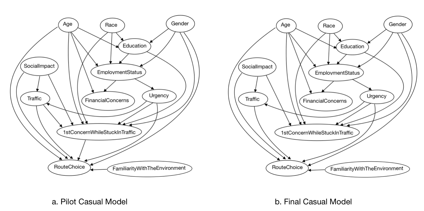
Figure 1: Casual Models

In the conditional independence test, our null hypothesis states that two variables are independent conditional on the other variable. So, if the $p$-value is greater than the significance level $\alpha$ = 0.01, we will accept our null hypothesis; otherwise we will reject it. After the test, it showed that some of the conditional independences implied by causal model were not consistent with the probability distribution underlying the dataset. For example, the result of conditional independence test against the dataset suggests that the variable of 1st concern while stuck in the traffic and the variable of route choice are independent conditioned on the variable of traffic. However, in the DAG, there is a direct edge between the variable of 1st concern while stuck in the traffic and the variable of route choice which is an indication of dependency. So we will eliminate this edge to make D-separation condition in the model match the conditional independence in the data.

Table 3: Some of the Conditional Independence Test

Conditional Independence	P-value ($\alpha$=0.01)
1stConcernWhileStuckInTraffic
and RouteChoice given Traffic	p=0.037
RouteChoice and 1stConcern-
WhileStuckInTraffic given Age	p=0.043
1stConcernWhileStuckInTraffic
and Education given Race	p=3.57E-10
Education and 1stConcernWhile-
StuckInTraffic given Gender	p$<$2.2E-16
1stConcernWhileStuckInTraffic
and RouteChoice given SocialImpact	p=0.504
RouteChoice and Traffic given
SocialImpact	p$<$2.2E-16
1stConcernWhileStuckInTraffic
and RouteChoice given Urgency	p=0.481
Traffic and 1stConcernWhile-
StuckInTraffic given Urgency	p=1
Education and EmploymentStatus
given Gender	p$<$2.2E-16
Education and EmploymentStatus
given Age	p$<$2.2E-16
Education and EmploymentStatus
given Race	p$<$2.2E-16
FinancialConcern and Employment-
Status given Age	p$<$2.2E-16

We concluded that the pilot model is not a good fit for the data set. To modify the pilot model, we could introduce new variables, remove redundant variables, or modify the relationship between variables by adding or eliminating nodes and edges. Based on the test results, we modified the pilot model by merely eliminating edges from the node of Traffic to the node of 1st concern while stuck in the traffic, and from the node of 1st concern while stuck in the traffic to the node of Route Choice. In the pilot DAG, there were $12$ nodes (variables) and 26 directed edges. In the final causal DAG, the number of nodes remain the same as in the pilot model, but $24$ directed edges remain. The pilot and final casual models are shown in Figure 1.

Causal effect estimation

The causal graph shows that between treatment-outcome pairs there is a direct path and an indirect (back-door) path (i.e, traffic $\rightarrow$ route choice is direct path; traffic $\leftarrow$ social impact $\rightarrow$ route choice is an indirect path). The back-door path is confounding. When trying to estimate causal effect, we want to block any back-door paths by conditioning on some variables, because such paths are not transmitting causal influences, and if we don’t block the back-door path, it confounds the effect that a node has on another node. For instance, as shown in Figure 2 (we boxed the collider with the dashed line and similarly presented the confounder’s arrows with dashed line), when trying to calculate the causal effect of employment status on route choice, there exists back-door paths: 1) employment status $\leftarrow$ education $\leftarrow$ gender $\rightarrow$ route choice; the blockage of this path can be ensured by conditioning on gender which is a confounder; 2) employment status $\leftarrow$ age $\rightarrow$ route choice; the blockage of this path can be ensured by conditioning on the confounder age; 3) employment status $\leftarrow$ race $\rightarrow$ 1st concern while stuck in the traffic $\leftarrow$ social impact $\rightarrow$ route choice; within the path there is a collider which is the variable of 1st concern while stuck in the traffic. So the back-door path is already blocked without conditioning on any variables. However, if we try to condition on the collider we make the path open instead. There are other back-door paths: we haven’t listed all of them. After identifying every back-door path between these two variables, we selected age and gender thereby blocking the back-door paths between employment status and route choice.

To select the variables that entail blockage of the the back-door paths, we carried out graph-surgery as described above. Then, we adjusted these variables to calculate the pure causal effect. We paired every treatment with the outcome variable, identified back-door paths between them, and selected the confounding variables using the Back-door criterion. Between the variables of Urgency, Gender, Race, Age, SocialImpact, FamiliarityWiththeEnvironment, and the RouteChoice there doesn’t exist any back-door path. In addition to that, from the variables of 1stConcernWhileStuckInTheTraffic, and FinancialConcern, there doesn’t exist any direct causal path to the variable of RouteChoice. So, there is no casual effect of these two variables on the variable of RouteChoice. The relationship between them can be interpreted as association instead of causation. Hence, there is no need to estimate the causal effect of these two variables. We listed the confounders in the the back-door paths between the variables of Traffic, Urgency, Education, EmploymentStatus and RouteChoice (Shown in Table 4). Normally, the strategy of putting in all possible confounders is usually used. However, this strategy may end up adjusting for colliders and mediators that can introduce bias. For example, employment status $\rightarrow$ urgency $\rightarrow$ route choice. In this direct path, urgency is mediator. if we condition on the mediator, we will bias our estimate.

Table 4: Confounder in Backdoor Paths

Variables	Confounder
Traffic	Urgency, SocialImpact
Urgency	Gender, Age
Education	Race, Gender, Age
EmploymentStatus	Gender, Age

We applied Inverse Probability(IP) weighting method to adjust the variables $Z$, which are the confounders. The purpose of using IP weighting is to break the association between the covariates $Z$ and treatment $X$ to estimate true causal effect on outcome variable $y$ Hernán  Robins (2006); Robins . (1994). By predicting $Z$ based on $X$, we can estimate the propensity score $\Pr(X=x|Z)$. We can get a propensity score using non-parametric (i.e, probability) or parametric methods (i.e, regression model). If the data is high-dimensional with many covariates and some of them with multiple levels, it is desirable to use a parametric method. In our study, we have 12 variables and some variables have more than two levels. To find propensity score, we applied logistic regression model. The equation is given below:

$$\Pr(X_{i}=x|Z_{i})=\dfrac{1}{1+e^{-\beta Z_{i}}}$$ (2)

After getting propensity scores, we used them to obtain the weights $W$ to create a pseudo-sample in which there is no association between the covariates and treatment. The IP weighting formula is given below:

$$W_{i}=\dfrac{X_{i}}{\Pr(X|Z_{i})}+\dfrac{1-X_{i}}{1-\Pr(X|Z_{i})}$$ (3)

where $X_{i}$ indicates if the $i$th subject was treated.

We started our approach of calculating the causal effect by training a model with covariates $Z$ to predict $X$. Our treatments $X$ are categorical variables, so we calculated the propensity scores $\Pr(X|Z)$ by applying equation 2.

After estimating the propensity scores, we applied equation 3 to obtain the $IP$ weight. We used stabilizing factor $\Pr(X)$ in the numerator to narrow the range of the $\Pr(X)/W$. After we obtained stabilized IP weights as $SW=\Pr(x)/W$, we trained new model with treatment variables $X$ as features and outcome Y by using $SW_{i}$ as sample weight for the $i$th observation. Then, we used this model to predict the causal effect. In this study, outcome variable is categorical data, so we used logistic regression again to obtain the casual odds ratio as a casual effect measure.

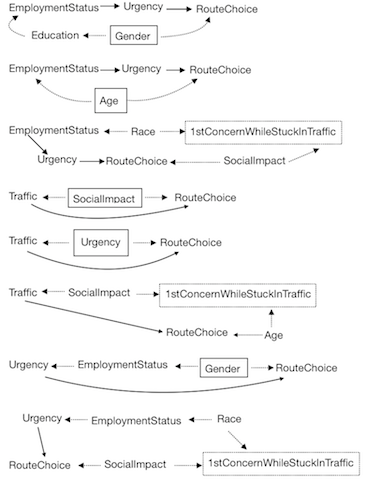
Figure 2: Blocking Backdoor

Table 5: Average Casual Estimation Result

Variables	ATE	95%Conf.Interval
SocialImpact
yes vs no	4.945	3.966 – 5.919
Urgency
Urgent vs Unurgent	1.193	0.773 – 1.612
Age
Middle vs Young	1.081	0.179 – 1.982
Old vs Young	0.461	-3.274 – 4.196
Gender
Male vs Female	0.976	0.135–1.816
Race
Middle Eastern vs White	5.760	4.587 – 6.932
Other vs White	3.966	2.750 – 5.181
EmploymentStatus
PartTime vs Unemployed	0.007	-6.049 – 7.651
FullTime vs Unemployed	0.015	-4.140 – 4.213
Student vs Unemployed	0.010	-4.471 – 4.582
Education
HighSchool vs PostGraduate	0.054	-2.431 – 2.539
College vs PostGraduate	1.231	0.825 – 1.636
Traffic
Medium vs Normal	3.663	1.953 – 5.372
Heavy vs Normal	6.562	4.817 – 8.306
FamilarityWithEnvironment
OnceAMonth vs OnceAWeek	2.795	0.938 – 4.651
OnceAYear vs OnceAWeek	2.778	1.374 – 4.181

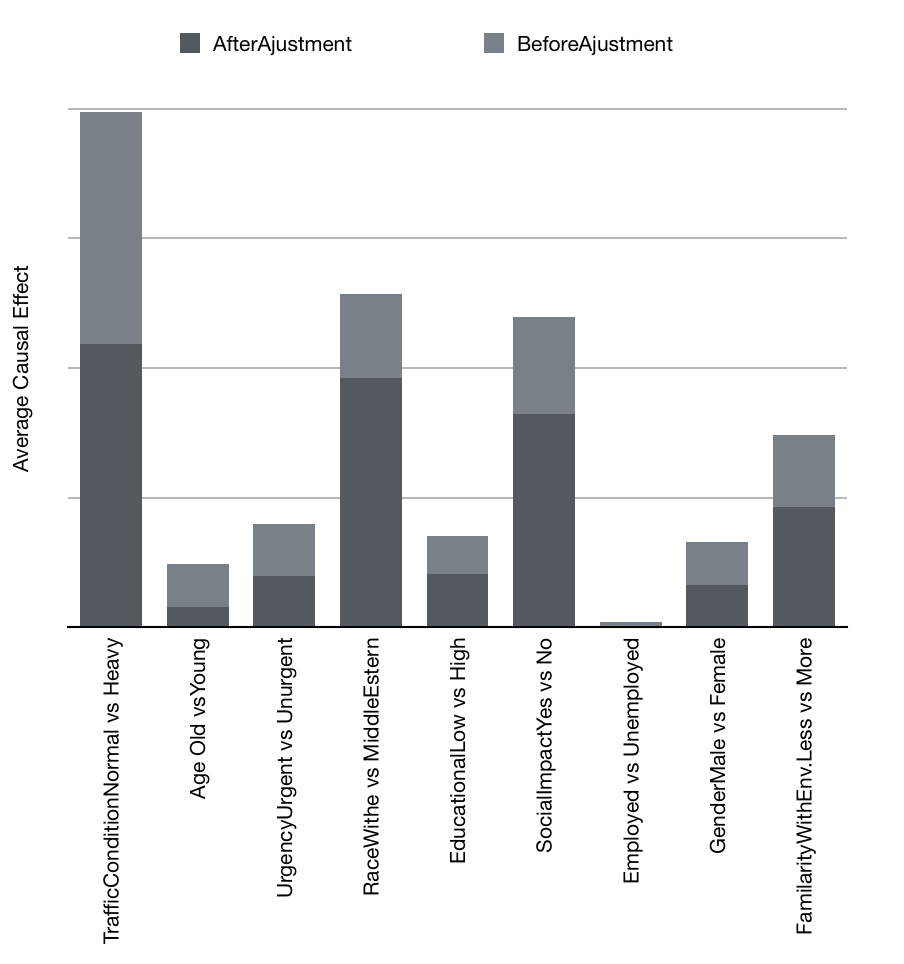
Figure 3: Average Causal Effects Of Variables Computed by Adjusted and Un-Adjusted Regression Model

Based on our determination of average causal effect (shown in Table 5), the result suggests that when heavy and medium traffic conditions are compared with the normal condition separately, their effects have significant magnitude. It implies that changes in traffic conditions impact drivers route choice. More specifically, when the traffic is heavy, proportion of drivers who choose the nearest exit is about $6$ times greater than that when traffic is normal. However, when the traffic is medium, proportion of drivers who choose the nearest exit is about $3$ times greater than that when traffic is normal. So, we can conclude that when the traffic is normal, the drivers are more likely to stay on the high way. Considering social impact, a driver would be influenced by watching other drivers take the exit. The proportion of drivers who choose the nearest exit is about $5$ times greater when they get influenced than they don’t. Considering familiarity with environment, proportion of drivers, who are not familiar with the road, choosing the nearest exit is about $3$ times greater than those who are familiar with the road. Considering race, white people are more likely to stay on the highway than middle eastern people or others. Age and Urgency also have significant effect on drivers route choice. We also conducted another experiment in which we built an estimator for route choice without adjusting for confounding factors, and compared the results with the one of causal inference (shown in Figure 3). The results suggest that on the un-adjusted estimator, the effect of age and employment status are overestimated, race, social impact, and familiarity with the environment are under estimated. This is because there are confounding and collider sources between the path of these variables and the outcome. Based on causal inference, the effect of traffic, race, social impact, and familiarity with the environment are more significant than others.

Conclusions

This paper described a causal analysis of route choice behavior of drivers using data collected from a Stated Choice Experiment in an Immersive Virtual Environment (IVE). This work will not only fill in the lack of causality based approaches in the transportation field, but it also showed that without adjustment on treatment, causal effect results will be affected by spurious correlation as well.

References

- Anderson \BBA Lenz (\APACyear\bibnodate) \APACinsertmetastarandlenz{APACrefauthors}Anderson, R\BPBID.\BCBT \BBA Lenz, R\BPBIT. \APACrefYearMonthDay\bibnodate. \BBOQ\APACrefatitleModeling the Impact of Organizational Change: A Bayesian Network Approach Modeling the impact of organizational change: A bayesian network approach.\BBCQ \APACjournalVolNumPagesOrganizational Research Methods. \PrintBackRefs\CurrentBib
- Basu, Ganguly\BCBL \BOthers. (\APACyear\bibnodate) \APACinsertmetastarbasu2015deepsat{APACrefauthors}Basu, S., Ganguly, S., Mukhopadhyay, S., DiBiano, R., Karki, M.\BCBL \BBA Nemani, R. \APACrefYearMonthDay\bibnodate. \BBOQ\APACrefatitleDeepsat: a learning framework for satellite imagery Deepsat: a learning framework for satellite imagery.\BBCQ \BIn \APACrefbtitleProceedings of the 23rd SIGSPATIAL international conference on advances in geographic information systems. Proceedings of the 23rd sigspatial international conference on advances in geographic information systems. \PrintBackRefs\CurrentBib
- Basu, Mukhopadhyay\BCBL \BOthers. (\APACyear\bibnodate) \APACinsertmetastarbasu2018deep{APACrefauthors}Basu, S., Mukhopadhyay, S., Karki, M., DiBiano, R., Ganguly, S., Nemani, R.\BCBL \BBA Gayaka, S. \APACrefYearMonthDay\bibnodate. \BBOQ\APACrefatitleDeep neural networks for texture classification?A theoretical analysis Deep neural networks for texture classification?a theoretical analysis.\BBCQ \APACjournalVolNumPagesNeural Networks. \PrintBackRefs\CurrentBib
- Ben-Akiva \BOthers. (\APACyear1985) \APACinsertmetastarben1985discrete{APACrefauthors}Ben-Akiva, M\BPBIE., Lerman, S\BPBIR.\BCBL \BBA Lerman, S\BPBIR. \APACrefYear1985. \APACrefbtitleDiscrete choice analysis: theory and application to travel demand Discrete choice analysis: theory and application to travel demand. \APACaddressPublisherMIT press. \PrintBackRefs\CurrentBib
- Ben-Akiva \BOthers. (\APACyear2004) \APACinsertmetastarben2004route{APACrefauthors}Ben-Akiva, M\BPBIE., Ramming, M\BPBIS.\BCBL \BBA Bekhor, S. \APACrefYearMonthDay2004. \BBOQ\APACrefatitleRoute choice models Route choice models.\BBCQ \BIn \APACrefbtitleHuman Behaviour and Traffic Networks. Human behaviour and traffic networks. \APACaddressPublisherSpringer. \PrintBackRefs\CurrentBib
- Ben-Elia \BBA Shiftan (\APACyear2010) \APACinsertmetastarben2010road{APACrefauthors}Ben-Elia, E.\BCBT \BBA Shiftan, Y. \APACrefYearMonthDay2010. \BBOQ\APACrefatitleWhich road do I take? A learning-based model of route-choice behavior with real-time information Which road do i take? a learning-based model of route-choice behavior with real-time information.\BBCQ \APACjournalVolNumPagesTransportation Research Part A: Policy and Practice. \PrintBackRefs\CurrentBib
- Dawid (\APACyear1979) \APACinsertmetastardawid1979conditional{APACrefauthors}Dawid, A\BPBIP. \APACrefYearMonthDay1979. \BBOQ\APACrefatitleConditional independence in statistical theory Conditional independence in statistical theory.\BBCQ \APACjournalVolNumPagesJournal of the Royal Statistical Society: Series B (Methodological). \PrintBackRefs\CurrentBib
- de Oñ \BOthers. (\APACyear2014) \APACinsertmetastarDeona{APACrefauthors}de Oñ, J., de Oña, R., Eboli, L., Forciniti, C.\BCBL \BBA Mazzulla, G. \APACrefYearMonthDay2014. \BBOQ\APACrefatitleHow to identify the key factors that affect driver perception of accident risk. A comparison between Italian and Spanish driver behavior How to identify the key factors that affect driver perception of accident risk. a comparison between italian and spanish driver behavior.\BBCQ \APACjournalVolNumPagesAccident Analysis & Prevention. \PrintBackRefs\CurrentBib
- Doherty \BBA Miller (\APACyear2000) \APACinsertmetastardoherty2000computerized{APACrefauthors}Doherty, S\BPBIT.\BCBT \BBA Miller, E\BPBIJ. \APACrefYearMonthDay2000. \BBOQ\APACrefatitleA computerized household activity scheduling survey A computerized household activity scheduling survey.\BBCQ \APACjournalVolNumPagesTransportation. \PrintBackRefs\CurrentBib
- Elwert (\APACyear2013) \APACinsertmetastarelwert2013graphical{APACrefauthors}Elwert, F. \APACrefYearMonthDay2013. \BBOQ\APACrefatitleGraphical causal models Graphical causal models.\BBCQ \BIn \APACrefbtitleHandbook of causal analysis for social research. Handbook of causal analysis for social research. \APACaddressPublisherSpringer. \PrintBackRefs\CurrentBib
- Elwert \BBA Winship (\APACyear2014) \APACinsertmetastarelwert2014endogenous{APACrefauthors}Elwert, F.\BCBT \BBA Winship, C. \APACrefYearMonthDay2014. \BBOQ\APACrefatitleEndogenous selection bias: The problem of conditioning on a collider variable Endogenous selection bias: The problem of conditioning on a collider variable.\BBCQ \APACjournalVolNumPagesAnnual review of sociology. \PrintBackRefs\CurrentBib
- Glymour \BBA Cooper (\APACyear1999) \APACinsertmetastarglymour1999computation{APACrefauthors}Glymour, C\BPBIN.\BCBT \BBA Cooper, G\BPBIF. \APACrefYear1999. \APACrefbtitleComputation, causation, and discovery Computation, causation, and discovery. \APACaddressPublisherAaai Press. \PrintBackRefs\CurrentBib
- Hernán \BBA Robins (\APACyear2006) \APACinsertmetastarhernan2006estimating{APACrefauthors}Hernán, M\BPBIA.\BCBT \BBA Robins, J\BPBIM. \APACrefYearMonthDay2006. \BBOQ\APACrefatitleEstimating causal effects from epidemiological data Estimating causal effects from epidemiological data.\BBCQ \APACjournalVolNumPagesJournal of Epidemiology & Community Health. \PrintBackRefs\CurrentBib
- Hernan \BBA Robins (\APACyear2018) \APACinsertmetastarhernan{APACrefauthors}Hernan, M\BPBIA.\BCBT \BBA Robins, J\BPBIM. \APACrefYear2018. \APACrefbtitleCausal inference Causal inference. \APACaddressPublisherBoca Raton : Chapman & Hall/CRC, forthcoming. \PrintBackRefs\CurrentBib
- Khattak \BOthers. (\APACyear1993) \APACinsertmetastarkhattak1993commuters{APACrefauthors}Khattak, A\BPBIJ., Schofer, J\BPBIL.\BCBL \BBA Koppelman, F\BPBIS. \APACrefYearMonthDay1993. \BBOQ\APACrefatitleCommuters’ enroute diversion and return decisions: analysis and implications for advanced traveler information systems Commuters’ enroute diversion and return decisions: analysis and implications for advanced traveler information systems.\BBCQ \APACjournalVolNumPagesTransportation Research Part A: Policy and Practice. \PrintBackRefs\CurrentBib
- LeCun \BOthers. (\APACyear\bibnodate) \APACinsertmetastarlecun2015deep{APACrefauthors}LeCun, Y., Bengio, Y.\BCBL \BBA Hinton, G. \APACrefYearMonthDay\bibnodate. \BBOQ\APACrefatitleDeep learning Deep learning.\BBCQ \APACjournalVolNumPagesnature521. \PrintBackRefs\CurrentBib
- Liu \BOthers. (\APACyear2019) \APACinsertmetastarqun{APACrefauthors}Liu, Q., Mukhopadhyay, S., Zhu, Y., Gudishala, R., Saeidi, S.\BCBL \BBA Nabijiang, A. \APACrefYearMonthDay2019. \BBOQ\APACrefatitleImproving Route Choice Models by Incorporating Contextual Factors via Knowledge Distillation Improving route choice models by incorporating contextual factors via knowledge distillation.\BBCQ \BIn \APACrefbtitleIn Proceedings of IEEE International Joint Conference on Neural Networks (IJCNN). In proceedings of ieee international joint conference on neural networks (ijcnn). \PrintBackRefs\CurrentBib
- Lv \BOthers. (\APACyear\bibnodate) \APACinsertmetastarlv2015traffic{APACrefauthors}Lv, Y., Duan, Y., Kang, W., Li, Z.\BCBL \BBA Wang, F\BHBIY. \APACrefYearMonthDay\bibnodate. \BBOQ\APACrefatitleTraffic flow prediction with big data: a deep learning approach Traffic flow prediction with big data: a deep learning approach.\BBCQ \APACjournalVolNumPagesIEEE Transactions on Intelligent Transportation Systems. \PrintBackRefs\CurrentBib
- Neapolitan \BOthers. (\APACyear2004) \APACinsertmetastarneapolitan2004learning{APACrefauthors}Neapolitan, R\BPBIE.\BCBT \BOthersPeriod. \APACrefYear2004. \APACrefbtitleLearning bayesian networks Learning bayesian networks. \APACaddressPublisherPearson Prentice Hall Upper Saddle River, NJ. \PrintBackRefs\CurrentBib
- Pearl (\APACyear2009) \APACinsertmetastarpearl2009causality{APACrefauthors}Pearl, J. \APACrefYear2009. \APACrefbtitleCausality Causality. \APACaddressPublisherCambridge university press. \PrintBackRefs\CurrentBib
- Pearl (\APACyear2014) \APACinsertmetastarpearl2014probabilistic{APACrefauthors}Pearl, J. \APACrefYear2014. \APACrefbtitleProbabilistic reasoning in intelligent systems: networks of plausible inference Probabilistic reasoning in intelligent systems: networks of plausible inference. \APACaddressPublisherElsevier. \PrintBackRefs\CurrentBib
- Pearl \BOthers. (\APACyear2016) \APACinsertmetastarpearl2016causal{APACrefauthors}Pearl, J., Glymour, M.\BCBL \BBA Jewell, N\BPBIP. \APACrefYear2016. \APACrefbtitleCausal inference in statistics: a primer Causal inference in statistics: a primer. \APACaddressPublisherJohn Wiley & Sons. \PrintBackRefs\CurrentBib
- Pearl \BBA Mackenzie (\APACyear2018) \APACinsertmetastaralma{APACrefauthors}Pearl, J.\BCBT \BBA Mackenzie, D. \APACrefYear2018. \APACrefbtitleThe book of why : the new science of cause and effect The book of why : the new science of cause and effect. \APACaddressPublisherBasic Books. \PrintBackRefs\CurrentBib
- Prato (\APACyear2009) \APACinsertmetastarprato2009route{APACrefauthors}Prato, C\BPBIG. \APACrefYearMonthDay2009. \BBOQ\APACrefatitleRoute choice modeling: past, present and future research directions Route choice modeling: past, present and future research directions.\BBCQ \APACjournalVolNumPagesJournal of choice modelling. \PrintBackRefs\CurrentBib
- Pursula \BBA Talvitie (\APACyear1993) \APACinsertmetastarpursula1993urban{APACrefauthors}Pursula, M.\BCBT \BBA Talvitie, A. \APACrefYearMonthDay1993. \BBOQ\APACrefatitleUrban route choice modelling with multinomial logit models Urban route choice modelling with multinomial logit models.\BBCQ \APACjournalVolNumPagesLIIKENNETEKNIIKKA, TIEDOTE. \PrintBackRefs\CurrentBib
- Robins \BOthers. (\APACyear1994) \APACinsertmetastarrobins1994estimation{APACrefauthors}Robins, J\BPBIM., Rotnitzky, A.\BCBL \BBA Zhao, L\BPBIP. \APACrefYearMonthDay1994. \BBOQ\APACrefatitleEstimation of regression coefficients when some regressors are not always observed Estimation of regression coefficients when some regressors are not always observed.\BBCQ \APACjournalVolNumPagesJournal of the American statistical Association. \PrintBackRefs\CurrentBib
- Scheines (\APACyear1997) \APACinsertmetastarscheines1997introduction{APACrefauthors}Scheines, R. \APACrefYearMonthDay1997. \BBOQ\APACrefatitleAn introduction to causal inference An introduction to causal inference.\BBCQ \PrintBackRefs\CurrentBib
- Song \BOthers. (\APACyear\bibnodate) \APACinsertmetastarsong2016deeptransport{APACrefauthors}Song, X., Kanasugi, H.\BCBL \BBA Shibasaki, R. \APACrefYearMonthDay\bibnodate. \BBOQ\APACrefatitleDeepTransport: Prediction and Simulation of Human Mobility and Transportation Mode at a Citywide Level. Deeptransport: Prediction and simulation of human mobility and transportation mode at a citywide level.\BBCQ \BIn \APACrefbtitleIJCAI. Ijcai. \PrintBackRefs\CurrentBib
- Spiegelhalter \BOthers. (\APACyear1993) \APACinsertmetastarspiegelhalter1993bayesian{APACrefauthors}Spiegelhalter, D\BPBIJ., Dawid, A\BPBIP., Lauritzen, S\BPBIL.\BCBL \BBA Cowell, R\BPBIG. \APACrefYearMonthDay1993. \BBOQ\APACrefatitleBayesian analysis in expert systems Bayesian analysis in expert systems.\BBCQ \APACjournalVolNumPagesStatistical science. \PrintBackRefs\CurrentBib