Relaxed 2-D Principal Component Analysis by $L_{p}$ Norm for Face Recognition

Abstract

A relaxed two dimensional principal component analysis (R2DPCA) approach is proposed for face recognition. Different to the 2DPCA, 2DPCA-$L_{1}$ and G2DPCA, the R2DPCA utilizes the label information (if known) of training samples to calculate a relaxation vector and presents a weight to each subset of training data. A new relaxed scatter matrix is defined and the computed projection axes are able to increase the accuracy of face recognition. The optimal $L_{p}$-norms are selected in a reasonable range. Numerical experiments on practical face databased indicate that the R2DPCA has high generalization ability and can achieve a higher recognition rate than state-of-the-art methods.

Key words. Face recognition; G2DPCA; Relaxed 2DPCA; Optimal algorithms; Alternating direction method

1 Introduction

The principal component analysis (PCA) [1, 2], has become one of the most powerful approaches of face recognition [3, 4, 5, 6, 7]. Recently, many robust PCA (RPCA) algorithms are proposed with improving the quadratic formulation, which renders PCA vulnerable to noises, into $L_{1}$-norm on the objection function, e.g., $L_{1}$-PCA [8], $R_{1}$-PCA [9], and PCA-$L_{1}$ [10]. Meanwhile, sparsity is also introduced into PCA algorithms, resulting in a series of sparse PCA (SPCA) algorithms [11, 12, 13, 14]. A newly proposed robust SPCA (RSPCA) [15] further applies $L_{1}$-norm both in objective and constraint functions of PCA, inheriting the merits of robustness and sparsity. Observing that $L_{2}$-, $L_{1}$-, and $L_{0}$-norms are all special $L_{p}$-norm, it is natural to impose $L_{p}$-norm on the objection or/and constraint functions, straightforwardly; see PCA-$L_{p}$ [16] and generalized PCA (GPCA) [17] for instance.

To preserve the spatial structure of face images, two dimensional PCA (2DPCA), proposed by Yang et al. [18], represents face images with two dimensional matrices rather than one dimensional vectors. The computational problems bases on 2DPCA are of much smaller scale than those based on traditional PCA, and the difficulties caused by low rank are also avoided. This image-as-matrix method offers insights for improving above RSPCA, PCA-$L_{p}$, GPCA, etc. As typical examples, the $L_{1}$-norm-based 2DPCA (2DPCA-$L_{1}$) [19] and 2DPCA-$L_{1}$ with sparsity (2DPCA$L_{1}$-S) [20] are improvements of PCA-$L_{1}$ and RSPCA, respectively, and the generalized 2DPCA (G2DPCA) [21] imposes $L_{p}$-norm on both objective and constraint functions of 2DPCA. Recently, the quaternion 2DPCA is proposed in [22] and applied to color face recognition, where the red, green and blue channels of a color image is encoded as three imaginary parts of a pure quaternion matrix. To arm the quaternion 2DPCA with the generalization ability, Zhao, Jia and Gong [23] proposed the sample-relaxed quaternion 2DPCA with applying the label information (if known) of training samples. The structure-preserving algorithms of quaternion eigenvalue decomposition and singular value decomposition can be found in [24, 25, 26, 27, 28, 29, 30, 31]. More applications of the quaternion representation and structure-preserving methods to color image processing can be found in [32] and [33].

Both PCA and 2DPCA are unsupervised methods and omit the potential or known label information of samples. They are often applied to the training set and thus the computed projections will maximize the scatter of projected training samples. That means the scatter of projected testing samples are not surely optimal, and certainly, so are the whole (training and testing) projected samples. Inspired by this observation, we proposed a new relaxation two-dimensional principal component analysis (R2DPCA) in this paper. R2DPCA sufficiently utilizes the labels (if known) of training samples, and can enhance the total scatter of whole projected samples. This approach is a generalization of G2DPCA [21], and will reduce to G2DPCA if the label information is unknown or unused.

The rest of this paper is organized as follows. In Section 2, we recall robust and sparse 2DPCA algorithms. In Section 3, we present a new relaxed two dimensional principal component analysis (R2DPCA) approach for face recognition. In Section 4, we compare the R2DPCA with the state-to-the-art approaches, and indicate the efficiencies of the R2DPCA . In Section 5, we sum up the contribution of this paper.

2 Robust and sparse 2DPCA algorithms

In this section, we recall 2DPCA, 2DPCA-$L_{1}$, 2DPCA$L_{1}$-S, and G2DPCA algorithms in the form of computing the first projection vector. In fact, after obtaining first $j$ projection vectors $\textbf{W}=[\textbf{w}_{1},\textbf{w}_{2},\ldots,\textbf{w}_{j}]$, the $(j+1)$-th projection vector $\textbf{w}_{j+1}$ can be calculated similarly on deflated samples [34]:

$$\textbf{X}_{i}^{deflated}=\textbf{X}_{i}(\textbf{I}-\textbf{W}\textbf{W}^{T}),i=1,2,\ldots,n.$$ (1)

2.1 2DPCA

Suppose that there are $n$ training images samples $\textbf{X}_{1},\textbf{X}_{2},\ldots,\textbf{X}_{n}\in\mathbb{R}^{h\times w}$, where $h$ and $w$ denote the height and width of images, respectively. We assume that these samples are mean-centered, i.e., $\frac{1}{n}\sum^{n}\nolimits_{i=1}\textbf{X}_{i}=0$; otherwise, we will replace $\textbf{X}_{i}$ by $\textbf{X}_{i}-\frac{1}{n}\sum^{n}\nolimits_{i=1}\textbf{X}_{i}$.

2DPCA [18] finds its first projection vector $\textbf{w}\in\mathbb{R}^{w}$ by solving the optimization problem with equality constraints:

$$\max\limits_{\textbf{w}\in\mathbb{R}^{w}}\sum\limits^{n}_{i=1}\|\textbf{X}_{i}\textbf{w}\|_{2}^{2},\ s.t.\|\textbf{w}\|_{2}^{2}=1.$$ (2)

The projection vector w could be calculated by the iterative algorithm:

$$\textbf{v}^{k}=\sum\limits^{n}_{i=1}\textbf{X}_{i}^{T}[|\textbf{X}_{i}\textbf{w}^{k}|\circ\texttt{sign}(\textbf{X}_{i}\textbf{w}^{k})],$$ (3a)

$$\textbf{u}^{k}=|\textbf{v}^{k}|\circ\texttt{sign}(\textbf{v}^{k}),$$ (3b)

$$\textbf{w}^{k+1}=\frac{\textbf{u}^{k}}{\|\textbf{u}^{k}\|_{2}},$$ (3c)

where sign$(\cdot)$ denotes the sign function. The projection vector w can also be obtained by calculating the eigen decomposition of a covariance matrix and selecting the eigenvector corresponding to the largest eigenvalue. See Remark 2.2 for more details.

2.2 2DPCA-$L_{1}$

2DPCA-$L_{1}$ [19] finds its first projection vector $\textbf{w}\in\mathbb{R}^{w}$ by solving the optimization problem with equality constraints:

$$\max\limits_{\textbf{w}\in\mathbb{R}^{w}}\sum\limits^{n}_{i=1}\|\textbf{X}_{i}\textbf{w}\|_{1},\ s.t.\|\textbf{w}\|_{2}^{2}=1.$$ (4)

The projection vector w could be calculated by the iterative algorithm:

$$\textbf{v}^{k}=\sum\limits^{n}_{i=1}\textbf{X}_{i}^{T}\texttt{sign}(\textbf{X}_{i}\textbf{w}^{k}),$$ (5a)

$$\textbf{w}^{k+1}=\frac{\textbf{v}^{k}}{\|\textbf{v}^{k}\|_{2}},$$ (5b)

where $\textbf{w}^{k}$ is the projection vector at the $k$-th step. Notice that 2DPCA-$L_{1}$ could be formulated by replacing the $L_{2}$-norm in objective function of 2DPCA with $L_{1}$-norm.

2.3 2DPCA$L_{1}$-S

2DPCA$L_{1}$-S [20] finds its first projection vector $\textbf{w}\in\mathbb{R}^{w}$ by solving the optimization problem with equality and inequality constraints:

$$\max\limits_{\textbf{w}\in\mathbb{R}^{w}}\sum\limits^{n}_{i=1}\|\textbf{X}_{i}\textbf{w}\|_{1},\ s.t.\|\textbf{w}\|_{1}\leq c,\|\textbf{w}\|_{2}^{2}=1,$$ (6)

where $c$ is a positive constant. The projection vector w could be calculated by the iterative algorithm:

$$\textbf{v}^{k}=\sum\limits^{n}_{i=1}\textbf{X}_{i}^{T}\texttt{sign}(\textbf{X}_{i}\textbf{w}^{k}),$$ (7a)

$$u_{i}^{k}=v_{i}^{k}\frac{|w_{i}^{k}|}{\lambda+|w_{i}^{k}|},\ i=1,2,\ldots,w,$$ (7b)

$$\textbf{w}^{k+1}=\frac{\textbf{u}^{k}}{\|\textbf{u}^{k}\|_{2}},$$ (7c)

where $u_{i}^{k}$, $v_{i}^{k}$, and $w_{i}^{k}$ are the $i$th elements of vectors $\textbf{u}^{k},\textbf{v}^{k},$ and $\textbf{w}^{k}\in\mathbb{R}^{w}$, respectively. In equation (7b), $\lambda$ is a positive scalar which serves as a tuning parameter. When $\lambda$ is set to be zero, 2DPCA$L_{1}$-S reduces to 2DPCA-$L_{1}$. Notice that 2DPCA$L_{1}$-S could be formulated by imposing $L_{1}$-norm on objective and constraint functions of 2DPCA.

2.4 G2DPCA

G2DPCA [21] finds its first projection vector $\textbf{w}\in\mathbb{R}^{w}$ by solving the optimization problem with equality constraints:

$$\max\limits_{\textbf{w}\in\mathbb{R}^{w}}\sum\limits^{n}_{i=1}\|\textbf{X}_{i}\textbf{w}\|_{s}^{s},\ s.t.\|\textbf{w}\|_{p}^{p}=1$$ (8)

where $s\geq 1$ and $p>0$. The projection vector w can be updated in two different ways, depending on the value $p$.

• Case 1: If $p\geq 1$,

  $$\textbf{v}^{k}=\sum\limits^{n}_{i=1}\textbf{X}_{i}^{T}[|\textbf{X}_{i}\textbf{w}^{k}|^{s-1}\circ\texttt{sign}(\textbf{X}_{i}\textbf{w}^{k})],$$ (9a)

  $$\textbf{u}^{k}=|\textbf{v}^{k}|^{q-1}\circ\texttt{sign}(\textbf{v}^{k}),$$ (9b)

  $$\textbf{w}^{k+1}=\frac{\textbf{u}^{k}}{\|\textbf{u}^{k}\|_{p}}.$$ (9c)

  where $q$ satisfies $1/p+1/q=1$, $\circ$ denotes the Hadamard product, i.e., the element-wise product between two vectors. Especially, if $p=1$, $\textbf{w}^{k+1}$ can be computed by

  $$j=\arg\max\nolimits_{i\in[1,w]}|v_{i}^{k}|,$$ (10a)

  $$w_{i}^{k+1}=\left\{\begin{aligned} \texttt{sign}(v_{j}^{k}),\ i=j,\\ 0,\ i\neq j,\\ \end{aligned}\right.$$ (10b)

  wherein $v_{i}^{k}$ is the $i$-th value of $\textbf{v}^{k}$; if $p=\infty$, $\textbf{w}^{k+1}$ can be computed by

  $$\textbf{w}^{k+1}=\texttt{sign}(\textbf{v}^{k}).$$ (11)

• Case 2: If $0<p<1$,

  $$\textbf{v}^{k}=\sum\limits^{n}_{i=1}\textbf{X}_{i}^{T}[|\textbf{X}_{i}\textbf{w}^{k}|^{s-1}\circ\texttt{sign}(\textbf{X}_{i}\textbf{w}^{k})],$$ (12a)

  $$\textbf{u}^{k}=|\textbf{w}^{k}|^{2-p}\circ\textbf{v}^{k},$$ (12b)

  $$\textbf{w}^{k+1}=\frac{\textbf{u}^{k}}{\|\textbf{u}^{k}\|_{p}}.$$ (12c)

Notice that G2DPCA could be formulated by generalizing $L_{2}$-norm in objective and constraint functions of 2DPCA to $L_{s}$-norm and $L_{p}$-norm, respectively.

Remark 2.1.

When $s=p=2$, the projection method (9) reduces to (3).

Remark 2.2.

By the eigenvalue decomposition method, 2DPCA can select a set of projection axes $\{\textbf{w}_{1},\textbf{w}_{2},\cdots,\textbf{w}_{r}\}$ in one step, without selecting only one optimal projection axis each step. These projection axes are chosen as eigenvectors of a covariant matrix corresponding to first $r$ largest eigenvalues:

$$\textbf{G}_{t}=\frac{1}{n}\sum\limits^{n}_{i=1}\textbf{X}_{i}^{T}\textbf{X}_{i},$$ (13a)

$$[\textbf{W},\textbf{D}]=\texttt{eig}(\textbf{G}_{t}),$$ (13b)

where $\textbf{G}_{t}$ is the covariance matrix of training samples, $\textbf{W}=[\textbf{w}_{1},\textbf{w}_{2},\cdots,\textbf{w}_{r}]\in R^{w\times r}$ is a matrix with unitary column vectors, D is a diagonal matrix consists of first $r$ largest eigenvalues. Since $G_{t}$ is symmetric and positive semi-definite, the diagonal elements of $D$ are nonnegative and the projection axes

$$\{\textbf{w}_{1},\textbf{w}_{2},\cdots,\textbf{w}_{r}\}=\arg\max\sum\limits^{n}_{i=1}\textbf{w}_{i}^{T}\textbf{G}_{t}\textbf{w}_{i},$$

are orthogonal to each other, i.e.,

$$\textbf{w}_{i}^{T}\textbf{w}_{j}=\left\{\begin{array}[]{l}1,~{}i=j,\\ 0,~{}i\neq j,\end{array}~{}s,t=1,\cdots,r.\right.$$ (14)

Remark 2.3.

We sum the procedures of above four methods in Table 1. Their relationship is also indicated in Fig 2.

Table 1: Procedures

Algorithm	2DPCA	2DPCA-$L_{1}$
Procedure	$[\textbf{W},\textbf{D}]=\texttt{eig}(\frac{1}{n}\sum\limits^{n}_{i=1}\textbf{X}_{i}^{T}\textbf{X}_{i})$	$\textbf{v}^{k}=\sum\limits^{n}_{i=1}\textbf{X}_{i}^{T}\texttt{sign}(\textbf{X}_{i}\textbf{w}^{k})$
		$\textbf{w}^{k+1}=\frac{\textbf{v}^{k}}{\|\textbf{v}^{k}\|_{2}}$
Algorithm	2DPCA$L_{1}$-S	G2DPCA
Procedure	$\textbf{v}^{k}=\sum\limits^{n}_{i=1}\textbf{X}_{i}^{T}\texttt{sign}(\textbf{X}_{i}\textbf{w}^{k})$	$\textbf{v}^{k}=\sum\limits^{n}_{i=1}\textbf{X}_{i}^{T}[|\textbf{X}_{i}\textbf{w}^{k}|^{s-1}\circ\texttt{sign}(\textbf{X}_{i}\textbf{w}^{k})]$
	$u_{i}^{k}=v_{i}^{k}\frac{|w_{i}^{k}|}{\lambda+|w_{i}^{k}|},\ i=1,2,\ldots,w$	if $p\geq 1$    run (9)
	$\textbf{w}^{k+1}=\frac{\textbf{u}^{k}}{\|\textbf{u}^{k}\|_{2}}$	if $0<p<1$    run (12)

3 The relaxed 2DPCA by $L_{p}$-norm

In this section, we introduce a relaxed two-dimensional principal component analysis (R2DPCA) method by $L_{p}$-norm. R2DPCA includes three parts: relaxation vector generation, objective function relaxation, and projection relaxation.

3.1 Relaxation vector

Suppose that training samples $\textbf{X}_{1},\textbf{X}_{2},...,\textbf{X}_{n}\in\mathbb{R}^{h\times w}$ can be partitioned into $m$ classes and each class contains $n_{j}$ samples:

$$\textbf{X}_{1}^{1},\cdots,\textbf{X}_{n_{1}}^{1}\ |\ \textbf{X}_{1}^{2},\cdots,\textbf{X}_{n_{2}}^{2}\ |\ \cdots\ |\ \textbf{X}_{1}^{m},\cdots,\textbf{X}_{n_{m}}^{m},$$

where $\textbf{X}_{i}^{j}$ denotes the $i$-th sample of the $j$-th class, $i=1,\ldots,n_{j}$, $j=1,\ldots,m$. Define the mean of training samples from the $j$-th class as

$$\textbf{M}_{j}=\frac{1}{n_{j}}\sum\limits_{i=1}^{n_{j}}\textbf{X}_{i}^{j}\in\mathbb{R}^{h\times w},$$

and the $j$-th within-class covariance matrix of the training set as

$$\textbf{C}_{j}=\frac{1}{n_{j}}\sum\limits_{i=1}^{n_{j}}(\textbf{X}_{i}^{j}-\textbf{M}_{j})^{T}(\textbf{X}_{i}^{j}-\textbf{M}_{j})\in\mathbb{R}^{w\times w},$$ (15)

where $j=1,\ldots,m$, $\sum_{j=1}^{m}n_{j}=n$ and $i=1,\ldots,n_{j}$.

The within-class covariance matrix $\textbf{C}_{j}$ is a symmetric and positive semi-definite matrix. Its maximal eigenvalue, denoted by $\lambda_{\max}(\textbf{C}_{j})$, represents the variance of training samples $\textbf{X}_{1}^{j},\ldots,\textbf{X}_{n_{j}}^{j}$ in the principal component. In general, the larger $\lambda_{\rm max}(\textbf{C}_{j})$ is, the better scattered of the training samples of $j$-th class are. A very small $\lambda_{\rm max}(\textbf{C}_{j})$ indicates that $\textbf{X}_{1}^{j},\ldots,\textbf{X}_{n_{j}}^{j}$ are not well scattered samples to represent the $j$-th class. Extremely, if $\lambda_{\max}(\textbf{C}_{j})=0$ then all of training samples from the $j$-th class are same, and then the contribution of the $j$-th class to the covariance matrix of training set should be controlled by a small factor. To this aim, we define a relaxation vector of training classes,

$$\textbf{v}=[v_{1},\cdots,v_{m}]^{T}\in\mathbb{R}^{m},$$ (16)

where

$$v_{j}=\frac{f(\lambda_{\rm max}(\textbf{C}_{j}))}{\sum_{i=1}^{m}f(\lambda_{\rm max}(\textbf{C}_{i}))},$$ (17)

is a relaxation factor of the $j$-th class with a function, $f:~{}\mathbb{R}\rightarrow\mathbb{R}^{+}$. A relaxation factor of each training sample of $j$-th class is defined as $v_{j}/n_{j}$. If each training class has only one sample, i.e., $n_{1}=\cdots=n_{m}=1$, then all within-class covariance matrices are zero matrix and $\lambda_{\max}(\textbf{C}_{1})=\cdots=\lambda_{\max}(\textbf{C}_{m})=0.$ In this case, the relaxation factor of each class is same ($v_{j}=1/m$), and so is the factor of each training sample of $j$-th class.

We sum above steps of computing the relaxation vector of training set in Algorithm 3.1.

Algorithm 3.1.

Relaxation vector generation

  function $\textbf{v}=\texttt{relaxvec}(\textbf{X}_{1},\textbf{X}_{2},\cdots,\textbf{X}_{n},m,w)$

  for $j=1,2,\cdots,m$ do

     $\textbf{C}_{j}=\texttt{zeros}(w,w);$

     $\textbf{M}_{j}=\frac{1}{n_{j}}(\textbf{X}_{1}^{j}+\cdots+\textbf{X}_{n_{j}}^{j});$

     for $i=1,2,\cdots,n_{j}$ do

        $\textbf{C}_{j}=\textbf{C}_{j}+{(\textbf{X}_{i}^{j}-\textbf{M}_{j})}^{\prime}*(\textbf{X}_{i}^{j}-\textbf{M}_{j});$

     end for

     $\textbf{C}_{j}=\textbf{C}_{j}/n_{j};$

     Compute relaxation vector v defined as in (16) and (17);

  end for

3.2 Objective function relaxation

Let M denote the mean of training samples, i.e.,

$$\textbf{M}=\frac{1}{n}\sum\limits^{n}_{i=1}\textbf{X}_{i}=\frac{1}{n}\sum\limits_{j=1}^{m}\sum\limits_{i=1}^{n_{j}}\textbf{X}_{i}^{j}.$$

With computed relaxation vector $\textbf{v}=$ $[v_{1},$ $\cdots,$ $v_{m}]^{T}$ in Section 3.1, we define a relaxed criterion as

$$J(\textbf{w})=\gamma\textbf{G}+(1-\gamma)\widetilde{\textbf{G}},$$ (18)

where $\gamma\in[0,1]$ is a relaxation parameter, $\textbf{w}\in\mathbb{R}^{w}$ is a unit vector under $L_{p}$ norm, $\textbf{G}:=\sum\limits^{n}_{i=1}\|(\textbf{X}_{i}-\textbf{M})\textbf{w}\|_{s}^{s}$ and $\widetilde{\textbf{G}}:=\sum\limits^{m}_{j=1}\sum\limits^{n_{j}}_{i=1}\|\frac{v_{j}}{n_{j}}(\textbf{X}_{i}^{j}-\textbf{M})\textbf{w}\|_{s}^{s}$. R2DPCA finds its first projection vector $\textbf{w}\in\mathbb{R}^{w}$ by solving the optimization problem with equality constraints:

$$\max\limits_{\textbf{w}\in\mathbb{R}^{w}}J(\textbf{w}),s.t.\|\textbf{w}\|_{p}^{p}=1,$$ (19)

where the criterion $J(\textbf{w})$ is defined as in (18). Notice that (19) reduces to (8) if $\gamma=1$, and thus, the first projection vector of R2DPCA is the same as that of G2DPCA. When $\gamma=0$, (19) is simplified as

$$\max\limits_{\textbf{w}\in\mathbb{R}^{w}}\sum\limits^{m}_{j=1}\sum\limits^{n_{j}}_{i=1}\|\frac{v_{j}}{n_{j}}(\textbf{X}_{i}^{j}-\textbf{M})\textbf{w}\|_{s}^{s},s.t.\|\textbf{w}\|_{p}^{p}=1.$$ (20)

If first $j$ projection vectors $\textbf{W}=[\textbf{w}_{1},\textbf{w}_{2},\ldots,\textbf{w}_{j}]$ have been obtained, the $(j+1)$-th projection vector $\textbf{w}_{j+1}$ can be calculated similarly on the deflated samples, defined as in (1). From each iterative step, we also obtain a maximized objective function value corresponding to $\textbf{w}_{j}$,

$$f_{j}=\gamma\sum\limits^{n}_{i=1}\|(\textbf{X}_{i}-\textbf{M})^{deflated}\textbf{w}_{j}\|_{s}^{s}+(1-\gamma)\sum\limits^{m}_{j=1}\sum\limits^{n_{j}}_{i=1}\|\frac{v_{j}}{n_{j}}(\textbf{X}_{i}^{j}-\textbf{M})^{deflated}\textbf{w}_{j}\|_{s}^{s}.$$

With the relaxed criterion defined in (18), first $r$ optimal projection vectors of R2DPCA solve the optimal problem with equality constraints:

$$\begin{array}[]{l}\{\textbf{w}_{1},\ldots,\textbf{w}_{r}\}=\arg\max J(\textbf{w})\\[5.0pt] \ {\rm s.t.}\ \ \left\{\begin{array}[]{l}\|\textbf{w}_{i}\|_{p}^{p}=1,\\ \textbf{w}_{i}^{T}\textbf{w}_{j}=0~{}i\neq j,\end{array}~{}i,j=1,\cdots,r.\right.\end{array}$$ (21)

We propose Algorithm 3.2 to compute first $r$ optimal projection vectors, $\textbf{W}=[\textbf{w}_{1},\cdots,\textbf{w}_{r}]$, and corresponding optimal objective function values, $\textbf{D}={\rm diag}(f_{1},\ldots,f_{r})$.

Algorithm 3.2.

R2DPCA

0:  $\textbf{X}_{1},\textbf{X}_{2},\cdots,\textbf{X}_{n},s\in[1,\infty),p\in(0,\infty],r,m,w,\gamma\in[0,1],n_{1},\cdots,n_{m},tol.$

0:  $\textbf{W}=[\textbf{w}_{1},\ldots,\textbf{w}_{r}],\textbf{D}=\texttt{diag}(f_{1},\ldots,f_{r}).$

  Initialize $\textbf{W}=[\ ]$, $\textbf{D}=[\ ]$.

  v=relaxvec($\textbf{X}_{1},\textbf{X}_{2},\cdots,\textbf{X}_{n},m,w$).

  Homogenize training samples.

  for $t=1,2,\cdots,r$ do

     Initialize $k=0$, $\delta=1$, arbitrary $\textbf{w}^{0}$ with $\parallel\textbf{w}^{0}\parallel_{p}=1$.

     $f_{0}=\gamma\sum\limits^{n}_{i=1}\|\textbf{X}_{i}\textbf{w}^{0}\|_{s}^{s}+(1-\gamma)\sum\limits^{m}_{j=1}\sum\limits^{n_{j}}_{j=1}\|\frac{v_{j}}{n_{j}}\textbf{X}_{i}^{j}\textbf{w}^{0}\|_{s}^{s}.$

     while $\delta>tol$ do

        $\textbf{v}^{k}=\gamma\sum\limits^{n}_{i=1}\textbf{X}_{i}^{T}[|\textbf{X}_{i}\textbf{w}^{k}|^{s-1}\circ\texttt{sign}(\textbf{X}_{i}\textbf{w}^{k})]+(1-\gamma)\sum\limits^{m}_{j=1}\sum\limits^{n_{j}}_{j=1}(\frac{v_{j}}{n_{j}}\textbf{X}_{i}^{j})^{T}[|\frac{v_{j}}{n_{j}}\textbf{X}_{i}^{j}\textbf{w}^{k}|^{s-1}\circ\texttt{sign}(\frac{v_{j}}{n_{j}}\textbf{X}_{i}^{j}\textbf{w}^{k})]$.

        Case 1: $0<p<1$

         $\textbf{u}^{k}=|\textbf{w}^{k}|^{2-p}\circ\textbf{v}^{k},$

         $\textbf{w}^{k+1}=\frac{\textbf{u}^{k}}{\parallel\textbf{u}^{k}\parallel_{p}}.$

        Case 2: $p=1$

         $j=\arg\max\nolimits_{i\in[1,w]}|v_{i}^{k}|,$

         $w_{i}^{k+1}=\left\{\begin{aligned} \texttt{sign}(v_{j}^{k}),\ i=j,\\ 0,\ i\neq j.\\ \end{aligned}\right.$

        Case 3: $1<p<\infty$

         $q=p/(p-1),$

         $\textbf{u}^{k}=|\textbf{v}^{k}|^{q-1}\circ\texttt{sign}(\textbf{v}^{k}),$

         $\textbf{w}^{k+1}=\frac{\textbf{u}^{k}}{\parallel\textbf{u}^{k}\parallel_{p}}.$

        Case 4: $p=\infty$

         $\textbf{w}^{k+1}=\texttt{sign}(\textbf{v}^{k}).$

        $f_{k+1}=\gamma\sum\limits^{n}_{i=1}\|\textbf{X}_{i}\textbf{w}^{k+1}\|_{s}^{s}+(1-\gamma)\sum\limits^{m}_{j=1}\sum\limits^{n_{j}}_{j=1}\|\frac{v_{j}}{n_{j}}\textbf{X}_{i}^{j}\textbf{w}^{k+1}\|_{s}^{s}.$

        $\delta=|f_{k+1}-f_{k}|/|f_{k}|.$

        $k\leftarrow k+1.$

     end while

     $\textbf{W}\leftarrow[\textbf{W},\textbf{w}^{k}].$

     $\textbf{D}=\texttt{diag}(\textbf{D},f_{k}).$

     $\textbf{X}_{i}=\textbf{X}_{i}(\textbf{I}-\textbf{W}\textbf{W}^{T}),i=1,2,\cdots,n.$

  end for

3.3 Projection relaxation

In Section 3.2, we obtain $r$ pairs of optimal values and projection vectors: $(f_{1},\textbf{w}_{1}),\ldots,(f_{r},\textbf{w}_{r})$. Define the feature image of sample $\textbf{X}_{i}$ under W as

$$\textbf{P}_{i}=(\textbf{X}_{i}-{\bf{M})}\textbf{W}\in\mathbb{R}^{w\times r},\ i=1,\cdots,n.$$ (22)

Each column of $\textbf{P}_{i}$, $\textbf{y}_{j}=(\textbf{X}_{i}-{\bf{M}})\textbf{w}_{j}$, is called the principal component (vector).

Now we use a nearest neighbour classifier for face recognition. For a given testing sample X, compute its feature image, $\textbf{P}=(\textbf{X}-{\bf{M}})\textbf{W}$. Find out the nearest training sample $\textbf{X}_{i}$ $(1\leq i\leq n)$ whose feature image minimizes

$$\|(\textbf{P}_{i}-\textbf{P})\textbf{D}\|_{2}.$$

Such $\textbf{X}_{i}$ is output as the person to be recognized.

The distance, $\|(\textbf{P}_{i}-\textbf{P})\textbf{D}\|_{2}=\|(\textbf{X}_{i}-\textbf{X})\textbf{W}\textbf{D}\|_{2}$, is called relaxed distance between $\textbf{X}_{i}$ and X. Compared with originally defined distance, such as in [21], each projection axe $\textbf{w}_{j}$ is relaxed by $f_{j}$ in classification process, $j=1,\cdots,r$.

3.4 Restarted alternating direction search method

In the R2DPCA approach of face recognition, we need choose optimal $L_{s}$- and $L_{p}$-norms to maximize the recognition or classification rate. The traverse method will cost a huge amount of computational time. Instead, we present a restarted alternating direction search method of searching optimal values of $s$ and $p$; see Algorithm 3.3.

Algorithm 3.3.

Restarted alternating direction search method

0:  A finite range of $(s,p)$: $\Omega=\{(s_{i},p_{j})|i,j=1,2,\cdots,N\}$, and a positive number $\delta$.

0:  $s,t$.

  Step 1. Choose a starter $(s_{i}^{0},p_{j}^{0})\in\Omega$, randomly, and compute the recognition rate, denoted as $\varrho^{0}(i,j)$.

  Step 2. With $p_{j}=p_{j}^{0}$, find the maximal recognition rate in $\{(s_{i},p_{j}^{0})|$ $i=1,2,\cdots,N\}$, denoted as $\varrho^{1/2}(i,j)$, and denote the maximum point as $(s_{i}^{1},p_{j}^{0})$.

  Step 3. With $s_{i}=s^{1}_{i}$, find the maximal recognition rate in $\{(s_{i}^{1},p_{j})|j=1,2,\cdots,$ $N\}$,denoted as $\varrho^{1}(i,j)$, and denote the maximum point as $(s_{i}^{1},p_{j}^{1})$.

  Step 4. If $\varrho^{1}(i,j)=\varrho^{0}(i,j)$ and $(s_{i}^{1},p_{j}^{1})=(s_{i}^{0},p_{j}^{0})$, go to Step 5; otherwise, let $(s_{i}^{0},p_{j}^{0})=(s_{i}^{1},p_{j}^{1})$ be a new starter, and go to Step 2.

  Step 5. Find the maximal recognition rate $\varrho^{2}(i,j)$ in $\{(s_{i},p_{j})||s_{i}-s_{i}^{1}|\leq\delta,|p_{j}-p_{j}^{1}|\leq\delta\}\cap\Omega$, and denote the maximum point as $(s_{i}^{2},p_{j}^{2})$.

  Step 6. If $\varrho^{2}(i,j)\leq\varrho^{1}(i,j)$, output $s=s_{i}^{1}$ and $p=p_{j}^{1}$; otherwise, let $(s_{i}^{0},p_{j}^{0})=(s_{i}^{2},p_{j}^{2})$ be a new starter, and go to Step 2.

If giving a enough large value $\delta$ in Algorithm 3.3, we can surely achieve the maximum value of recognition rate at optimal values $(s_{j}^{2},p_{j}^{2})\in\Omega$. The selecting process is indicated in Fig 1.

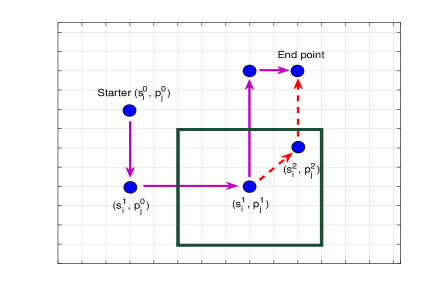
Figure 1: The searching path of restarted alternating direction search method

3.5 Mathematical theory of R2DPCA

R2DPCA is a generalization of G2DPCA [21]. As one of PCA-based methods, G2DPCA does not use the labels of data which possibly can impair class discrimination. To improve this, R2DPCA utilizes labels of training samples and variances within class to generate a relaxation vector, computes optimal projections maximizing the relaxes criterion, and thus enhances the class discrimination.

The working principle of R2DPCA can be clearly explained through a special case that $p=s=2$. The relaxed criterion with $L_{2}$-norm is also called generalized total scatter criterion, and has the form:

$$J(\textbf{W})={\rm trace}(\textbf{W}^{T}(\gamma\textbf{G}+(1-\gamma)\widetilde{\textbf{G}})\textbf{W})=\sum_{i=1}^{r}\textbf{w}_{i}^{T}(\gamma\textbf{G}+(1-\gamma)\widetilde{\textbf{G}})\textbf{w}_{i},$$ (23)

where

G $$=\frac{1}{n}\sum_{i=1}^{n}(\textbf{X}_{i}-{\bf{M}})^{T}(\textbf{X}_{i}-{\bf{M}}),$$ (24a)

$$\widetilde{\textbf{G}} =\sum_{j=1}^{m}\left(\frac{v_{j}}{n_{j}}\sum_{i=1}^{n_{j}}(\textbf{X}_{i}^{j}-{\bf{M}})^{T}(\textbf{X}_{i}^{j}-{\bf{M}})\right),$$ (24b)

where $\textbf{W}=[\textbf{w}_{1},\cdots,\textbf{w}_{r}]$ has orthogonal columns and each column is unitary under $L_{p}$-norm, $v_{j}$ is the $j$-th element of the relaxation vector v. Here $\sum_{j=1}^{m}n_{j}=n$. Recall that ${\bf{M}}\in\mathbb{R}^{h\times w}$ is the mean of training samples. Let $\textbf{W}^{opt}=[\textbf{w}_{1}^{opt},\cdots,\textbf{w}_{r}^{opt}]$ be the optimal projection, where $\textbf{w}_{1}^{opt},\cdots,\textbf{w}_{r}^{opt}$ solve the optimal problem (21). These optimal projection axes are in fact the orthogonal eigenvectors of $\gamma\textbf{G}+(1-\gamma)\widetilde{\textbf{G}}$ corresponding to first $r$ largest eigenvalues. Since the matrix $\gamma\textbf{G}+(1-\gamma)\widetilde{\textbf{G}}$ is symmetric and positive semi-definite, $J(\textbf{W})$ is nonnegative.

R2DPCA with $s=p=2$ can also be seen as applying the relaxation idea to 2DPCA, and thus called relaxed 2DPCA. Algorithm 3.2 with $s=2,p=2$ is one method of processing the relaxed 2DPCA. Another method is applying the eigenvalue decomposition (Algorithm 3.4 ), as shown in Remark 2.2.

Algorithm 3.4.

relaxed 2DPCA.

0:  $\textbf{X}_{1},\textbf{X}_{2},\cdots,\textbf{X}_{n},\textbf{M},s=p=2,r,m,w.$

0:  $\textbf{W},\textbf{D}$.

  $\textbf{v}=\texttt{relaxvec}(\textbf{X}_{1},\textbf{X}_{2},\cdots,\textbf{X}_{n},m,w);$

  $\textbf{G}=\texttt{zeros}(w,w);$

  Compute G and $\widetilde{\textbf{G}}$ defined as in (24).

  $[\textbf{W},\textbf{D}]=\texttt{eig}(\gamma\textbf{G}+(1-\gamma)\widetilde{\textbf{G}});$

  $\textbf{W}=\textbf{W}(:,1:r);\textbf{D}=\texttt{diag}(\textbf{D}(1:r)).$

Remark 3.1.

If there is no label information or people don’t want to use it, then let $m=n$ (thus, $v_{j}=1/n,~{}n_{j}=1$) or $m=1$ (thus, $v_{j}=1,~{}n_{j}=n$), $\widetilde{\textbf{G}}$ defined in (24b) is exactly the total scatter matrix (24a) defined for the classic 2DPCA just like the case $\gamma=1$.

Now we focus on the relationships among 2DPCA, 2DPCA$L_{1}$, 2DPCA$L_{1}$-S , G2DPCA, and R2DPCA. It is obvious that 2DPCA and 2DPCA-$L_{1}$ are two special cases of G2DPCA. 2DPCA$L_{1}$-S originates from G2DPCA with $s=1$ and $p=1$ which leads to projection vector with only one nonzero element. Then the $L_{2}$-norm constraint is employed to fix this problem, resulting in 2DPCA$L_{1}$-S. On the other hand, G2DPCA with $s=1$ and $1<p<2$ behaves like 2DPCA$L_{1}$-S, since the $L_{p}$-norm constraint in G2DPCA behaves like the mixed-norm constraint in 2DPCA$L_{1}$-S. Applying the relaxation idea to 2DPCA, 2DPCA$L_{1}$ and 2DPCA$L_{1}$-S, we can get three special cases of R2DPCA. To get a better understanding of these relationships, we construct a relationship graph in Fig 2.

Figure 2: relationship graph.

4 Experiments

In this section, we present numerical experiments to compare the proposed relaxed two dimensional principle component analysis (R2DPCA) by $L_{p}$-norm with state-of-the-art algorithms on face recognition. Three famous databases are utilized:

• Faces95 database (1440 images from 72 subjects, twenty images per subject),

• color Feret database (3025 images from 275 subjects, eleven images per subject),

• grey Feret database (1400 images from 200 subjects, seven images per subject).

All of face images are cropped and resized, and each image is of 80$\times$80 size. The numerical experiments are performed with MATLAB-R2016 on a personal computer with Intel(R) Xeon(R) CPU E5-2630 v3 @ 2.4GHz (dual processor) and RAM 32GB.

Example 4.1.

In this experiment, we compare R2DPCA with 2DPCA, 2DPCA-$L_{1}$, 2DPCA$L_{1}$-S, and G2DPCA. We randomly select $10$ and $5$ images of each person from Faces95 database and color Feret face database as the training set, respectively, and the remaining as the testing set. As in [21] we set $\Omega=\{(s,p)|s=1.0:0.1:3.0,p=0.9:0.1:3.0\}$ for G2DPCA and R2DPCA. The parameter $\rho$ of 2DPCA$L_{1}$-S relates to the $\lambda$ in [11] via $\lambda=10^{-\rho}$ is tuned, consistent with [20]. The optimal $\rho$ value is selected from $[-3.0:0.1:3.0]$. Here, the relaxed parameter of criterion in (18) is set as $\gamma=0$ and the number of eigenfaces is fixed as $r=10$ (Other cases will be considered in Examples 4.2-4.3).

We repeat the whole procedure two times and output the average recognition rate. The face recognition rate (Accuracy) and corresponding optimal parameter are listed in Table 2 and Table 3, respectively. The reasonable trend of the classification accuracies according to different choices of $s$ and $p$ is presented in Fig 3 and Fig 4. These numerical results indicate that R2DPCA performs better than other four state-of-art algorithms.

Table 2: Classification accuracies of five algorithms on faces95

$Algorithms$	$Optimalparameters$	$Accuracy$
2DPCA	$-$	$0.8729$
2DPCA-$L_{1}$	$-$	$0.8708$
2DPCA$L_{1}$-S	$\rho=-0.5$	$0.8785$
G2DPCA	$s=2.7,p=2.2$	$0.9451$
R2DPCA $(\gamma=0)$	$s=1,p=2.2$	0.9493

Table 3: Classification accuracies of five algorithms on Color Feret

$Algorithms$	$Optimalparameters$	$Accuracy$
2DPCA	$-$	$0.5982$
2DPCA-$L_{1}$	$-$	$0.5985$
2DPCA$L_{1}$-S	$\rho=-0.3$	$0.6236$
G2DPCA	$s=2.8,p=2.6$	$0.6918$
R2DPCA $(\gamma=0)$	$s=3,p=2.2$	0.7085

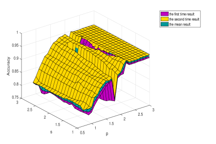
Figure 3: Classification accuracies with $s,p$ on Faces95.

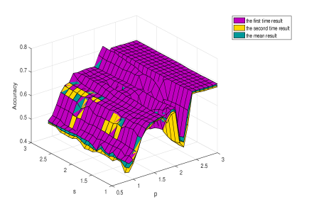
Figure 4: Classification accuracies with $s,p$ on Color Feret.

Example 4.2.

In this experiment, we research the effect of the parameter $\gamma$ of R2DPCA on the classification accuracy. The first $10$ and $5$ images of each person are selected as the training sets of the Faces95 and color/gray Feret face databases, respectively; and $r=10$ features are selected.

The results with several representative values $\gamma$ are shown in Table 4 and Table 5. We can see that the Faces95 and color FERET databases are not sensitive to $\gamma$, and however, we can see the validity of the parameters $\gamma$ on the Gray Feret database.

Table 4: Classification accuracies according to different $\gamma$ on faces95.

Database	$\gamma$	Optimal parameters	Accuracy
faces95	$0:1/4:1$	$s=1.1,p=2.2$	${\bf 0.8861}$
color FERET	$0:1/4:3/4$	$s=3,p=2.2$	$0.7673$
	$1$	$s=3,p=2.2$	${\bf 0.7733}$

Table 5: Classification accuracies according to different $\gamma$ on Gray Feret.

$\gamma$	Optimal parameters	Accuracy
$0$	$s=1.8,p=1.7$	$0.6075$
$1/4$	$s=1.9,p=1.7$	$0.6075$
$1/2$	$s=2.3,p=1.6$	${\bf 0.6112}$
$3/4$	$s=2.4,p=1.6$	$0.6088$
$1$	$s=2.6,p=1.8$	$0.5837$

Example 4.3.

In this experiment, we test the effect of numbers of chosen features on the classification accuracy. We randomly select $10,5$ images of each subject as training samples and the remaining as testing samples on the Faces95 and Color Feret databases, respectively. The whole procedure is repeated two times and the average accuracies are listed. Based on the optimal parameters $s,p$ of R2DPCA with $\gamma=0$ in Example 4.1, we set $s=1,~{}~{}p=2.2$ and $s=3,~{}~{}p=2.2$.

Fig 5 and Fig 6 show the classification accuracies of G2DPCA and R2DPCA with different feature numbers in the range of $[1,30]$ on the Faces95 database and Color Feret database, respectively. From these results, we can see that the classification accuracies of R2DPCA are higher and more stable than G2DPCA. When $k=1$ the classification accuracies of G2DPCA and R2DPCA are the same, which consists to the theory.

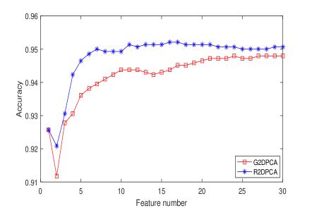
Figure 5: Classification accuracies of R2DPCA and G2DPCA with $k=[1:30]$ on Faces95.

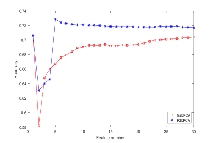
Figure 6: Classification accuracies of R2DPCA and G2DPCA with $k=[1:30]$ on Color Feret.

Example 4.4.

In this experiment, we research the influence of parameters $s$, $p$ on classification accuracies of R2DPCA with the case $\gamma=0$.

The training sets and testing sets just like Example 4.1. The classification accuracies with $10$ feature numbers, then the results are recorded. The procedure is repeated two times and then we take the average value. We use the optimal parameters of each databases on R2DPCA in Example 4.1. Here we fix $s=1$ and search the optimal parameters set from $p=[0.9:0.1:3.0]$ on the Faces95 database. We fix $s=3$ and search the optimal parameters set from $p=[0.9:0.1:3.0]$ on the Color Feret database. Similarly, we fix $p=2.2$ and search the optimal parameters set from $s=[1.0:0.1:3.0]$ on the Faces95 database. We fix $p=2.2$ and search the optimal parameters set from $s=[1.0:0.1:3.0]$ on the Color Feret database.

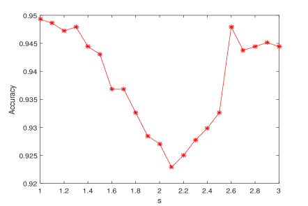
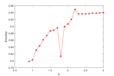
Figure 7: Classification accuracies of R2DPCA with $s$ and $p$ on Faces95.

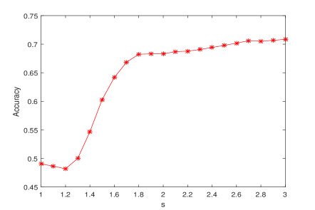
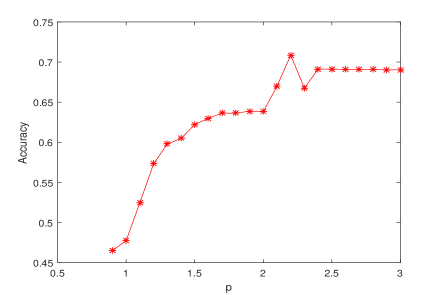
Figure 8: Classification accuracies of R2DPCA with $s$ and $p$ on Color Feret.

The results are shown in Fig 7 and Fig 8. From these Figures, we know that when $s=1,p=2.2$, the accuracy classification approach to maximum on the Faces95 database. When $s=3,p=2.2$, the accuracy classification approach to maximum on the Color Feret database. These results are consistent with the results of Experiment 4.1. And from these figures, we also can know that the accuracy classification do not have a stable variation trend with $s$ or $p$.

Example 4.5.

In section 3.4, we proposed a restarted alternating direction search method. Now we test this method on the Faces95 database and Color Feret database. From Example 4.4, we know the classification accuracies don’t have a stable trend with different $s$ or $p$. Traditionally, we need to traverse all the combinations of $s,p$, so that we can get the maximum solution. This way spends large time of calculations. Here, we test the restarted alternating direction search method.

$\Omega=\{(s,p)|s=1.0:0.1:3.0,p=0.9:,0.1:3.0\}$ is set as in [21]. We randomly use $10,5$ images of each subject as the training samples and the remaining images as the testing samples to do this restarted alternating direction search algorithm. We randomly start from four initial points, i.e., $s=1,s=1.6,p=0.9,p=1.2$ to find corresponding starters and then find the max classification accuracy of R2DPCA. We set a value $s$ (or $p$) to find a value $p$ (or $s$) and use $(s,p)$ as a starter. We set $\delta=0.3$ to control time. We do R2DPCA with $\gamma=0$ and obtain the max classification accuracy $0.9375,0.7158$ on two databases respectively. In order to have a more intuitive view of searching paths, we describe the results in Table 6 and Table 7.

From section 3.4, if $\varrho^{1}(i,j)=\varrho^{0}(i,j)$ and $(s_{i}^{1},p_{j}^{1})=(s_{i}^{0},p_{j}^{0})$, we should go to Step 5 to do a restarted algorithm. This situation occurs in this experiment. For example, in table 6, we can see that if starter is $s=1,p=2.2$, we make a restarted algorithm in the next step. Because of a small positive value $\delta=0.3$, it can’t reach to the new starter correspond to the next max accuracy which can be seen from the second row in this table. If we set a enough bigger positive value $\delta$, it can search the optimal solution. Due to this property, we can use this algorithm to do a pre computation with databases which needed to be identified, so that we can have a general idea of whether these databases are applicable to the algorithms we proposed.

In each two databases, we should do Algorithm 3.2 462 times in traditional R2DPCA. But now we at most do Algorithm 3.2 153 times and even do 3 times at least. And there is a little difference between observed results and true accuracies.

Table 6: Restarted alternating searching path on Face95.

$initial~{}~{}~{}~{}point$	$path$	$searching~{}~{}~{}~{}Accuracy$
$s=1,p=2.2$	$(1,2.2)$	$0.9347$
$s=1.3,p=0.9$	$(1.3,0.9)\rightarrow(1.3,2.1)\rightarrow(1.8,2.1)$	0.9375
$s=1.6,p=2.8$	$(1.6,2.8)\rightarrow(1.3,2.8)$	$0.9306$
$s=2.7,p=1.2$	$(2.7,1.2)\rightarrow(2.7,2.2)\rightarrow(1,2.2)\rightarrow(1,2.1)\rightarrow(1.8,2.1)$	0.9375

Table 7: Restarted alternating searching path on Color Feret.

$initial~{}~{}~{}point$	$path$	$searching~{}~{}~{}~{}Accuracy$
$s=1,p=2.4$	$(1,2.4)\rightarrow(2.7,2.4)\rightarrow(2.7,2.2)$	0.7158
$s=1.7,p=0.9$	$(1.7,0.9)\rightarrow(1.7,2.3)\rightarrow(1.6,2.3)\rightarrow(1.6,2.6)\rightarrow(2.5,2.6)\rightarrow(2.5,2.1)$	$0.7085$
$s=1.6,p=1.7$	$(1.6,1.7)\rightarrow(2.5,2.7)\rightarrow(2.5,2.2)\rightarrow(2.5,2.2)\rightarrow(2.7,2.2)$	0.7158
$s=1.2,p=1.2$	$(1.2,1.2)\rightarrow(1.2,2.3)$	$0.6939$

Example 4.6.

This method is common to 2DPCA-like methods. Now we compare the results of algorithms including 2DPCA, 2DPCA-$L_{1}$, 2DPCA$L_{1}$-S with their relaxation results on Gray Feret database.

We randomly select $tr=3$ training samples from each subject and the remaining images as testing samples. Here, we also choose 10 feature numbers to save computational time. Then the nearest neighbour classifier is applied to do classification. Also, the procedure is repeated two times and take the average classification accuracies. Notice that the relaxed 2DPCA Algorithm 3.4 as shown in Remark 2.2 and the other two algorithms’ relaxed progression are similar with R2DPCA Algorithm 3.2. In order to be consistent with the previous experimental parameters, we set $\gamma=0$. The results see Table 8.

Table 8: classification accuracies of six algorithms on Gray FERET

$Algorithms$	$Optimalparameters$	$Accuracy$
2DPCA	$-$	$0.4225$
R2DPCA $(s=p=2)$	$-$	0.6387
2DPCA-$L_{1}$	$-$	$0.4225$
R2DPCA$(s=1,p=2)$	$-$	0.6123
2DPCA$L_{1}$-S	$\rho=-0.6$	$0.4938$
R2DPCA $(s=1)$	$\rho=-2$	0.5988

From the results, we can know that our proposed R2DPCA algorithm is also effective for other 2-D algorithms.

Example 4.7.

We test the accuracies of the Gray Feret database with the number of training samples in this example.

We randomly select $tr=3$ training samples from each subject and the remaining images as testing samples. Here, we also choose 10 feature numbers. Then the nearest neighbor classifier is applied to do classification. We do this process two times and take the average classification accuracies in Fig 9. Also, in order to be consistent with the previous experimental parameters, we set $\gamma=0$.

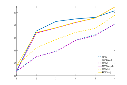
Figure 9: Accuracy with the number of training samples on Gray Feret database.

From this Figure, we known that the classification accuracies of relaxed versions are higher than those in original versions.

5 Conclusion

In this paper, we present a relaxed two dimensional principal component analysis (R2DPCA) approach for face recognition, with applying the label information of the training data. The R2DPCA is a generalization of 2DPCA, 2DPCA-$L_{1}$ and G2DPCA, and has higher generalization ability. Since utilizing the label information, the R2DPCA can be seen as a new supervised projection method, but it is totally different to the two-dimensional linear discriminant analysis (2DLDA)[35, 36].

References

- [1] I. Jolliffe (2004) Principal Component Analysis, New York, NY, USA: Springer.
- [2] M. Turk, A. Pentland (1991) Eigenfaces for recognition, J. Cogn. Neurosci., 3 (1), pp. 71-86.
- [3] L. Sirovich, M. Kirby (1987) Low-dimensional procedure for characterization of human faces, J. Optical Soc. Am. 4, pp. 519-524.
- [4] M. Kirby, L. Sirovich (1990) Application of the karhunenloeve procedure for the characterization of human faces, IEEE Trans. Pattern Anal. Mach. Intell., 12 (1), pp. 103-108.
- [5] M. Turk, A. Pentland (1991) Eigenfaces for recognition. J. Cognitive Neurosci, 3(1), pp. 71-76.
- [6] L. Zhao, Y. Yang (1999) Theoretical analysis of illumination in PCA-based vision systems, Pattern Recogn., 32(4), pp. 547-564.
- [7] A. Pentland (2000) Looking at people: sensing for ubiquitous and wearable computing, IEEE Trans. Pattern Anal. Mach. Intell., 22 (1), pp. 107-119.
- [8] Q. Ke and T. Kanade (2005) Robust norm factorization in the presence of outliters and missing data by alternative convex programming, Proc. IEEE Conf. Comput. Vis. Pattern Recognit., 1, San Diego, CA, USA, pp. 739-746.
- [9] C. Ding, D. Zhou, X. He, and H. Zha (2006) -PCA: Rotational invariant -norm principal component analysis for robust subspace factorization, Proc. 23rd Int. Conf. Mach. Learn., Pittsburgh, PA, USA, pp. 281-288.
- [10] N. Kwak (2008) Principal component analysis based on -norm maximization, IEEE Trans. Pattern Anal. Mach. Intell., 30 (9), pp. 1672-1680.
- [11] H. Zou, T. Hastie, and R. Tibshirani (2006) Sparse principal component analysis, J. Comput. Graph. Stat., 15 (2), pp. 265-286.
- [12] A. d’Aspremont, L. EI Ghaoui, M. I. Jordan, and G. R. Lanckriet (2007) A direct formulation for sparse PCA using semidefinite programming, SIAM Rev., 49 (3), pp. 434-448.
- [13] H. Shen and J. Z. Huang (2008) Sparse principal component analysis via regularized low rank matrix approximation, J. Multivar. Anal., 99 (6), pp. 1015-1034.
- [14] D. M. Witten, R. Tibshirani, and T. Hastie (2009) A penalized matrix decomposition, with applications to sparse principal components and canonical correlation analysis, Biostatistics, 10 (3), pp. 515-534.
- [15] D. Meng, Q. Zhao, and Z. Xu (2012) Improve robustness of sparse PCA by -norm maximization, Pattern Recognit., 45 (1), pp. 487-497.
- [16] N. Kwak (2014) Principal component analysis by -norm maximization, IEEE Trans. Cybern., 44 (5), pp. 594-609.
- [17] Z. Liang, S. Xia, Y. Zhou, L. Zhang, and Y. Li (2013) Feature extraction based on -norm generalized principal component analysis, Pattern Recognit. Lett., 34 (9), pp. 1037-1045.
- [18] J. Yang, D. Zhang, A. F. Frangi, J. Y. Yang (2004) Two-dimensional PCA: A new approach to appearance-based face representation and recognition, IEEE Trans. Pattern Anal. Mach. Intell., 26 (1), pp. 131-137.
- [19] X. Li, Y. Pang, and Y. Yuan (2010) -norm-based 2DPCA, IEEE Trans. Syst., Man, Cybern. B, Cybern., 40 (4), pp. 1170-1175.
- [20] H. Wang and J. Wang (2013) 2DPCA with -norm for simultaneously robust and sparse modelling, Neural Netw., 46, pp. 190-198.
- [21] J. Wang (2016) Generalized 2-D Principal Component Analysis by -Norm for Image Analysis, IEEE Transactions on cybernetics., 46 (3), pp. 792-803.
- [22] Z. Jia, S. Ling, M. Zhao (2017) Color two-dimensional principal component analysis for face recognition based on quaternion model, LNCS, vol. 10361, pp. 177-189.
- [23] M. Zhao, Z. Jia, D. Gong (2018) Sample-relaxed two-dimensional color principal component analysis for face recognition and image reconstruction, arXiv.org/cs /arXiv:1803.03837v1, 10 Mar 2018.
- [24] Z. Jia, M. Wei, S. Ling (2013) A new structure-preserving method for quaternion Hermitian eigenvalue problems, J. Comput. Appl. Math. 239, pp. 12-24.
- [25] R. Ma, Z. Jia, Z. Bai (2018) A structure-preserving Jacobi algorithm for quaternion Hermitian eigenvalue problems, Comput. Math. Appl., 75(3), pp. 809-820.
- [26] Z. Jia, R. Ma, M. Zhao (2017) A New Structure-Preserving Method for Recognition of Color Face Images, Computer Science and Artificial Intelligence , pp. 427-432.
- [27] Z. Jia, M. Wei, M. Zhao, Y. Chen (2018) A new real structure-preserving quaternion QR algorithm, J. Comput. Appl. Math. 343, pp. 26-48.
- [28] Z Jia, X Cheng, M Zhao (2009) A new method for roots of monic quaternionic quadratic polynomial, Comput. Math. Appl. 58(9), pp. 1852-1858.
- [29] Z. Jia, Q. Wang, M. Wei (2010) Procrustes problems for (P, Q, )-reflexive matrices, J. Comput. Appl. Math. 233(11), pp. 3041-3045.
- [30] M. Zhao, Z. Jia (2014) Structured least-squares problems and inverse eigenvalue problems for (P, Q)-reflexive matrices, Appl. Math. Comput. 235, pp. 87-93.
- [31] Z. Jia, M.K. Ng, G. Song (2018) Lanczos method for large-scale quaternion singular value decomposition, Numer. Algorithms, 08 November 2018. https://doi.org/10.1007/s11075-018-0621-0
- [32] Z. Jia, M.K. Ng, and G. Song (2019) Robust Quaternion Matrix Completion with Applications to Image Inpainting, Numer. Linear Algebra Appl., DOI:10.1002/nla.2245. http://www.math.hkbu.edu.hk/ mng/quaternion.html
- [33] Z. Jia, M.K. Ng, and W. Wang (2019) Color Image Restoration by Saturation-Value (SV) Total Variation, SIAM J. Imaging Sci., accepted. http://www.math.hkbu.edu.hk/ mng/publications.html
- [34] L. Mackey (2008) Deflation methods for sparse PCA, Proc. Adv. Neural Inf. Process. Syst., 21, Whistler, BC, Canada., pp. 1017-1024.
- [35] J. Ye (2005) Characterization of a family of algorithms for generalized discriminant analysis on undersampled problems, Machine Learning Res., pp. 483-502.
- [36] Z.Z. Liang, Y.F. Li, P.F. Shi (2008) A note on two-dimensional linear discriminant analysis, Pattern Recognit. Lett. 29, pp. 2122-2128.