Quantum Non-demolition Measurement of a Many-Body Hamiltonian

Abstract

In an ideal quantum measurement, the wave function of a quantum system collapses to an eigenstate of the measured observable, and the corresponding eigenvalue determines the measurement outcome. If the observable commutes with the system Hamiltonian, repeated measurements yield the same result and thus minimally disturb the system. Seminal quantum optics experiments have achieved such quantum non-demolition (QND) measurements of systems with few degrees of freedom. In contrast, here we describe how the QND measurement of a complex many-body observable, the Hamiltonian of an interacting many-body system, can be implemented in a trapped-ion analog quantum simulator. Through a single-shot measurement, the many-body system is prepared in a narrow band of (highly excited) energy eigenstates, and potentially even a single eigenstate. Our QND scheme, which can be carried over to other platforms of quantum simulation, provides a framework to investigate experimentally fundamental aspects of equilibrium and non-equilibrium statistical physics including the eigenstate thermalization hypothesis and quantum fluctuation relations.

I Introduction

Recent experimental advances provide intriguing opportunities in the preparation, manipulation, and measurement of the quantum state of engineered complex many-body systems. This includes the ability to address individual sites of lattice systems enabling single-shot read-out of single-particle observables, as demonstrated by the quantum gas microscope for atoms in optical lattices Parsons1253 ; Boll1257 , single-spin or qubit read-out of trapped ions Brydges2018 ; Garttner2017 ; Negnevitsky:2018aa ; Rossnagel325 ; Landsman:2019aa and Rydberg tweezers arrays Norcia2018 ; Cooper2018 ; Keesling:2019aa ; Barredo:2018aa ; PhysRevLett.122.143002 , and superconducting qubits Barends2016 ; PhysRevX.8.021003 . In contrast, we are interested below in developing single-shot measurements of many-body observables such as the Hamiltonian $\hat{H}$ of an interacting many-body system. For an isolated quantum system, $\hat{H}$ represents a QND observable, and our goal is to implement a QND measurement of energy of a quantum many-body system in an analog simulator setting. We note that quantum optics provides with several examples of QND measurements; however these have so far been confined to observables representing few quantum degrees of freedom Gleyzes2007 ; Johnson2010 ; Volz2011 ; PhysRevX.8.021003 ; Hacohen-Gourgy:2016aa ; PhysRevLett.99.120502 ; Eckert:2007aa .

Developing QND measurement of a many-body Hamiltonian $\hat{H}$ provides us first of all with the unique opportunity to distill—in a single run of the experiment—an energy eigenstate $\ket{\ell}$ from an initial, possibly mixed, or finite temperature state, by observing in particular run the energy eigenvalue $E_{\ell}$. In case of measurement with finite resolution, this will prepare states in a narrow energy window, reminiscent of a microcanonical ensemble. We emphasize that state preparation by measurement is intrinsically probabilistic, i.e., will vary from shot to shot, reflecting the population distribution. Furthermore, this provides us with a tool to determine populations and population distributions of (excited) energy eigenstates, as required in, e.g., many-body spectroscopy Senko430 . The ability to prepare and measure (single) energy eigenstates provides us with a unique tool to address experimentally fundamental problems in quantum statistical physics, such as the eigenstate thermalization hypothesis (ETH) Deutsch1991 ; Srednicki1994 ; Rigol:2008aa , which asserts that single energy eigenstates of an (isolated) ergodic system encode thermodynamic equilibrium properties. Developing the capability to turn QND measurements on and off allows one to alternate between time periods of free evolution of the unobserved many-body quantum system, and energy measurement. This allows quantum feedback in a many-body system conditional to measurement outcomes, and in particular provides a framework to monitor non-equilibrium dynamics and processes in quantum thermodynamics Campisi2011 , including measurement of work functions and quantum fluctuation relations (QFRs) PhysRevLett.101.070403 ; An:2014aa ; Cerisola:2017aa . These relations express fundamental constraints on, e.g. the work performed on a quantum system in an arbitrary non-equilibrium process, imposed by the universal canonical form of thermal states and the principle of microreversibility.

Our aim below is to develop QND measurement of $\hat{H}$ in physical settings of analog quantum simulation, in particular exploring the regime of mesoscopic system sizes. We will demonstrate this in detail for the example of an analog trapped-ion quantum simulator, realizing a long-range transverse Ising Hamiltonian and the associated QND measurement. Our implementation in an analog quantum device should be contrasted to QND measurement of $\hat{H}$ via a phase estimation algorithm McArdle2018 , which however requires a universal (digital) quantum computer.

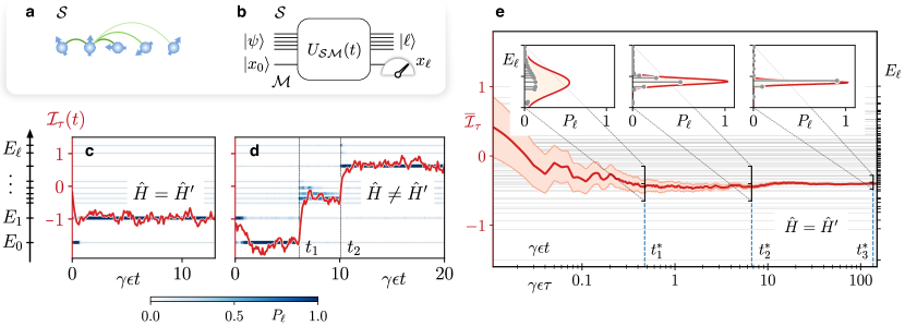
Figure 1: QND measurement of a many-body Hamiltonian $\hat{H}$ in a quantum simulator setting. The many-body spin system $\mathcal{S}$, shown in (a), is entangled with an ancillary system $\mathcal{M}$ (meter) by the unitary $\hat{U}_{\mathcal{SM}}(t)=\exp\{-i\int_{0}^{t}dt^{\prime}[\hat{H}\otimes\mathbb{I}+\vartheta(t^{\prime})\hat{H}\otimes\hat{P}]\}$. (b) Subsequent reading of a meter value $x_{\ell}\equiv x_{0}+E_{\ell}\int_{0}^{t}dt^{\prime}\vartheta(t^{\prime})$ prepares the many-body system in an energy eigenstate $\ket{\ell}$ with the eigenvalue $E_{\ell}$. (c) Single trajectory simulation (4), (5) of an ideal QND measurement for the Ising Hamiltonian (3) for $N=5$ spins, $\alpha=1.5$, $h/J=1.5$. The window-filtered homodyne current $\mathcal{I}_{\tau}(t)$ (red curve) fluctuates around a value corresponding to the eigenenergy prepared by the measurement of $\hat{H}$. The thin horizontal lines show the system eigenenergies $E_{\ell}$ and the blue color indicates the conditional populations $P_{\ell}(t)$ of the corresponding eigenstates. (d) Observation of quantum jumps due to the mismatch of the transverse fields $\hat{H}^{\prime}=\hat{H}+\delta\tilde{h}\sum_{j}\hat{\sigma}_{j}^{z}$ with $\smash{\delta\tilde{h}/J=-0.2}$. The filtered photocurrent (red) clearly shows sudden jumps between eigenstates at times $t_{1}$ and $t_{2}$. (e) Preparation of energy eigenstates or microcanonical ensembles by the ideal QND measurement for $N=8$ spins, $\alpha=1.5$, $h/J=0.8$. The estimate of the system energy given by the cumulative time-average of the homodyne current $\overline{\mathcal{I}}_{\tau}$ (red line) gradually converges to a single eigenenergy (grey lines) as averaging time $\tau$ increases. The corresponding uncertainty (red area) due to shot noise decreases as $\sim 1/\sqrt{\gamma\epsilon\tau}$. Inset: conditional population of the energy eigenstates (grey points) at times $t_{1}^{*}$, $t_{2}^{*}$, and $t_{3}^{*}$ is well captured by gaussian distributions of widths $J/\sqrt{4\gamma\epsilon t_{1,2,3}^{*}}$ describing the fluctuations of the shot noise averaged over $\tau=t_{1,2,3}^{*}$ (red curve).

II Results

II.1 QND Measurement of $\hat{H}$

On a more formal level, we define QND measurement of a many-body Hamiltonian $\hat{H}$ as an indirect measurement by coupling the system of interest $\mathcal{S}$, illustrated in Fig. 1(a), to an ancillary system $\mathcal{M}$ as meter. In a first step, the system is entangled with the meter according to the time evolution $U(t)=\exp(-i\hat{H}_{{\rm QND}}t)$ generated by the QND Hamiltonian

$$\hat{H}_{{\rm QND}}=\vartheta\hat{H}\otimes\hat{P},$$ (1)

with coupling strength $\vartheta$ ($\hbar=1$). To be specific and in light of examples below, we consider here as meter a continuous variable system with a pair of conjugated quadratures $\hat{X}$ and $\hat{P}$ obeying the canonical commutation relation $\smash{[\hat{X},\hat{P}]=i}$. Consider now an initial state of the joint system prepared as $\ket{\Psi}=\ket{\psi}\otimes\ket{x_{0}}$, where $\ket{\psi}\equiv\sum_{\ell}c_{\ell}\ket{\ell}$ is a superposition of energy eigenstates, $\hat{H}\ket{\ell}=E_{\ell}\ket{\ell},$ and $\ket{x_{0}}$ is an (improper) eigenstate of $\hat{X}$ (or squeezed state). We obtain for the time-evolved state $\ket{\Psi(t)}=\hat{U}(t)\ket{\psi}\otimes\ket{x_{0}}=\sum_{\ell}c_{\ell}\ket{\ell}\otimes\ket{x_{0}+\vartheta E_{\ell}t}$. Reading the meter as $x_{\ell}\equiv x_{0}+\vartheta E_{\ell}t$, and thus measuring the eigenvalue $E_{\ell}$, will prepare the system in $\ket{\ell}$ (or in the relevant subspace in case of degeneracies). The probability for obtaining the particular measurement outcome $E_{\ell}$ is $P_{\ell}=|c_{\ell}|^{2}$. Repeating the QND measurement will reproduce the particular $E_{\ell}$ with certainty, with the system remaining in $\ket{\ell}$. The above discussion is readily extended to mixed initial system states, and to initial meter states e.g. as coherent states.

In an analog quantum simulator setting, QND measurement of the many-body Hamiltonian $\hat{H}$ is incorporated by engineering the extended system-meter Hamiltonian $\hat{H}_{\mathcal{SM}}=\hat{H}\otimes\mathbb{I}+\vartheta\hat{H}\otimes\hat{P}$. In an interaction picture with respect to $\hat{H}\otimes\mathbb{I}$, the joint system then evolves according to the Hamiltonian $\hat{H}_{\mathcal{SM}}^{{\rm int}}\equiv\hat{H}_{{\rm QND}}$ realising the QND measurement discussed above and illustrated in Fig. 1(b). On the other hand, by allowing the system–meter coupling $\vartheta(t)$ to be switched on and off in time, we can alternate between the conventional free-evolution simulation and QND measurement mode of the system. In an actual implementation, as discussed below for trapped ions, we will achieve building the extended system-meter Hamiltonian

$$\hat{H}_{\mathcal{SM}}=\hat{H}^{\prime}\otimes\mathbb{I}+\vartheta\hat{H}\otimes\hat{P},$$ (2)

where $\hat{H}^{\prime}$ and $\hat{H}$ may differ (slightly). We note that the QND measurement of $\hat{H}$ is obtained by fine-tuning $\smash{\hat{H}^{\prime}=\hat{H}}$. A mismatch $\smash{\hat{H}^{\prime}\neq\hat{H}}$ will be visible as quantum jumps between energy eigenstates in repeated measurements.

In the trapped-ion example discussed below the many-body Hamiltonian $\hat{H}$ will be a long-range transverse Ising model Zhang2017 ; Britton2012 ; Jurcevic:2014aa ; Porras2004 ,

$$\hat{H}=-\sum_{i<j}^{N}J_{ij}\hat{\sigma}_{i}^{x}\hat{\sigma}_{j}^{x}-h\sum_{j}^{N}\hat{\sigma}_{j}^{z},$$ (3)

where $J_{ij}=J/\left\lvert i-j\right\rvert^{\alpha}$ with $\smash{0<\alpha<3}$ and $h$ the transverse field. Remarkably, in our implementation, the Hamiltonian $\hat{H}^{\prime}$ will differ from $\hat{H}$ just by the transverse field taking on the value $h^{\prime}$. We will be able to tune $h=h^{\prime}$ thus achieving the QND condition.

As last step in our formal development, we wish to formulate QND measurement of $\hat{H}$ as measurement continuous in time Wade2015 ; Mazzucchi2016 ; Ashida2017 ; Lee2014 . Physically, this amounts to making frequent and, in a continuum limit, continuous readouts $X(t)$ of the meter variable $\hat{X}$, with the quantum many-body system evolving according to (2). Following a well-established formalism of quantum optics Gardiner2015 ; Wiseman2010a we write for the system under continuous observation a stochastic master equation (SME) for a conditional density matrix $\hat{\rho}_{\rm c}(t)$ of the many-body system. In our context this SME reads

$$d\hat{\rho}_{\rm c}(t)= -i[\hat{H}^{\prime},\hat{\rho}_{\rm c}(t)]dt+\gamma\mathcal{D}[\hat{H}/J]\hat{\rho}_{\rm c}(t)\,dt$$

$$+\sqrt{\gamma\epsilon}\mathcal{H}[\hat{H}/J]\hat{\rho}_{\rm c}(t)\,dW(t),$$ (4)

$$dX(t)\equiv I(t)dt=2\sqrt{\gamma\epsilon}\langle\hat{H}/J\rangle_{\rm c}dt+dW(t).$$ (5)

with $dW(t)$ a Wiener increment, to be interpreted as an Itô stochastic differential equation. In a quantum optical setting, as in the ion trap example below, $I(t)$ is identified with photocurrent in homodyne detection of scattered light Gardiner2015 . Monitoring the photocurrent $\smash{I(t)\sim\langle\hat{H}\rangle_{\rm c}}$ thus provides continuous read out of the many-body Hamiltonian $\hat{H}$ with $\left\langle\ldots\right\rangle_{\rm c}\equiv{\rm Tr}[\ldots\hat{\rho}_{\rm c}(t)]$ up to shot noise. Thus $\hat{\rho}_{\rm c}(t)$ describes the many-body quantum state conditional to observing a particular photocurrent trajectory $I(t)$, as can be observed in a single run of an experiment. In (4) and (5) $\gamma$ is an effective measurement rate, and $\epsilon$ is a measurement efficiency. Furthermore, we have defined a Lindblad superoperator $\mathcal{D}[\hat{s}]\hat{\rho}_{\rm c}\equiv\hat{s}\hat{\rho}_{\rm c}\hat{s}^{\dagger}-(\hat{s}^{\dagger}\hat{s}\hat{\rho}_{\rm c}+\mathrm{H.c.})/2$ describing decoherence due to the quantum measurement backaction, and the nonlinear superoperator $\mathcal{H}[\hat{s}]\hat{\rho}_{\rm c}\equiv(\hat{s}-\langle\hat{s}\rangle_{\rm c})\hat{\rho}_{\rm c}+\mathrm{H.c.}$ which updates the density matrix conditioned on the observation of the homodyne photocurrent. Finally, not reading the meter, i.e. averaging over all measurement outcomes $I(t)$, the SME (4) reduces to a master equation with Lindblad term $\smash{\sim\mathcal{D}[\hat{H}]\hat{\rho}}$, i.e. realizing a reservoir coupling with jump operator $\hat{H}$, which erases all off-diagonal terms of the averaged density matrix $\hat{\rho}$ in the energy eigenbasis.

Equations (4), (5) allow us to simulate single measurement runs corresponding to a stochastic trajectory $I(t)$. Fig. 1(c) illustrates ideal QND measurement, $\smash{\hat{H}^{\prime}=\hat{H}}$, of the Hamiltonian (3) by plotting a sample trajectory of a filtered photocurrent, obtained by averaging $I(t)$ over a time window $\tau$, $\mathcal{I}_{\tau}(t)=(2N\sqrt{\gamma\epsilon}\tau)^{-1}\int_{0}^{\infty}dt^{\prime}I(t-t^{\prime})e^{-t^{\prime}/\tau}$. As initial condition we take all spins pointing against the transverse field. As seen in Fig. 1(c) the trajectory $\mathcal{I}_{\tau}(t)$ (red curve) stabilizes on a time scale $\sim\gamma^{-1}$ on a particular energy eigenvalue $E_{\ell}$ of (3) (up to fluctuations from shot noise). In this figure we consider and show only the eigenstates and eigenenergies (thin horizontal lines) within the symmetry sector containing the ground state of the Ising model with $J,\,h>0$, see Methods. The collapse, and thus preparation of the many-body wavefunction in the corresponding energy eigenstate is indicated by plotting the populations $P_{\ell}(t)\equiv\bra{\ell}\hat{\rho}_{\rm c}(t)\ket{\ell}$ [blue shadings in Fig. 1(c)]. Figure 1(d) shows quantum jumps between energy eigenstates induced by $\hat{H}^{\prime}\neq\hat{H}$. For weak perturbation ($\big{|}[\hat{H}^{\prime},\hat{H}]\big{|}\ll|\hat{H}|^{2}$) there are rare jumps between the energy eigenstates, indicated as $t_{1}$ and $t_{2}$ for the trajectory in Fig. 1(d). Finally, Fig. 1(e) plots the integrated current $\overline{\mathcal{I}}_{\tau}=(2N\sqrt{\gamma\epsilon}\tau)^{-1}\int_{0}^{\tau}I(t)dt$ and its fluctuations as a function of total integration time $\tau$. For $N=8$ spins starting in a thermal state the integrated current $\overline{\mathcal{I}}_{\tau}$ (red curve) exhibits a collapse at a rate $\smash{\sim\gamma}$ to a particular energy eigenstate. The insets shows the probabilities $P_{\ell}$ for various times, and the narrowing of the energy resolution as $\Delta E/J\sim 1/\sqrt{\gamma\epsilon\tau}$ with growing $\tau$ (see Methods); first to small energy window containing a few eigenstates as in a microcanonical ensemble, and eventually to a single energy eigenstate.

II.2 Implementation with Trapped Ions

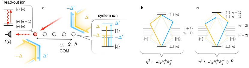
Figure 2: Trapped-ion implementation of the system-meter Hamiltonian $\hat{H}_{\mathcal{SM}}$. (a) Ion string with $N$ system ions (white) illuminated by four laser beams in a double Mølmer-Sørensen configuration. As described in the text this generates $\hat{H}_{\mathcal{SM}}$ [see Eq. (2)] with transverse Ising Hamiltonians $\hat{H^{\prime}}$ (6) and $\hat{H}$ (3), and the meter variable $\hat{P}$ representing the COM motion. The meter variable $\hat{X}$ is read by driving one, or potentially several ancilla ions (red) with a laser (red beam) tuned to the red motional COM sideband (see text). Homodyne detection of the scattered light to read $\hat{X}$, and thus revealing $\hat{H}$ in the photocurrent $I(t)\sim\langle\hat{H}\rangle_{\rm c}$ [see Eq. (5)]. (b) Level scheme of a pair of ions sharing the COM phonon mode, illustrating one of the elementary processes contributing to the Ising term $-\sum_{i<j}J_{ij}\hat{\sigma}_{i}^{x}\hat{\sigma}_{j}^{x}\otimes\mathbb{I}$ in second order in $\eta$. (c) Level scheme showing the corresponding third order processes contributing to $-\vartheta\sum_{i<j}J_{ij}\hat{\sigma}_{i}^{x}\hat{\sigma}_{j}^{x}\otimes\hat{P}$ (see text).

We now provide a trapped ion implementation of the system-meter Hamiltonian $\hat{H}_{\mathcal{SM}}$ (2). As shown in Fig. 2(a), we consider a string of $N$ ions in a linear Paul trap representing spin-1/2 $\left\{\left|\downarrow\right\rangle_{i},\left|\uparrow\right\rangle_{i}\right\}$. These two-level ions can be driven by laser light $\left|\downarrow\right\rangle\rightarrow\left|\uparrow\right\rangle$, where the recoil associated with absorption and emission of photons provides a coupling to vibrational eigenmodes of the ion chain. This includes in particular the center-of-mass motion (COM) with $\hat{X}$ and $\hat{P}$ position and momentum operators, respectively, which play the role of meter variables.

To generate in $\hat{H}_{\mathcal{SM}}$ both the Ising interaction $-\sum_{i<j}J_{ij}\hat{\sigma}_{i}^{x}\hat{\sigma}_{j}^{x}\otimes\mathbb{I}$, as well as the Ising term coupled to COM, $-\vartheta\sum_{i<j}J_{ij}\hat{\sigma}_{i}^{x}\hat{\sigma}_{j}^{x}\otimes\hat{P}$, we choose a laser configuration consisting of two pairs of counterpropagating laser beams [c.f. Fig. 2(a)]. In generalization of Sorensen1999 ; Molmer1999 we call this a double Mølmer-Sørensen configuration. The first pair of MS beams (shown as amber in Fig. 2) is detuned by $\pm\Delta$ from ionic resonance, while the second pair (blue) is detuned by $\pm\Delta^{\prime}$. Furthermore, we choose $\Delta^{\prime}-\Delta=\omega_{0}$ with $\omega_{0}$ the COM frequency. These four laser beams give rise to laser induced two-photon processes involving pairs of ions, which are depicted in Figs. 2(b,c).

First, as shown in Fig. 2(b), absorption of a photon from the one of the amber MS laser beam followed by an absorption from the counterpropagating amber beam gives rise to a two-photon excitation $\ket{\downarrow\downarrow}\rightarrow\ket{\uparrow\uparrow}$, which is resonant with twice the (bare) ionic transition frequency of the two-level ion. We emphasize that this process leaves the motional state of the ion chain unchanged, as illustrated by $\ket{n}\rightarrow\ket{n}$ for the COM mode with $n$ the phonon occupation number. This process will thus contributes a term $\sim\hat{\sigma}_{i}^{+}\hat{\sigma}_{j}^{+}$ to the effective spin-spin interaction. The second pair of MS beams (blue) will again contribute a resonant two-photon excitation, which adds coherently to the first contribution. By considering all possible processes, we obtain the effective Ising interaction $-\sum_{i<j}J_{ij}\hat{\sigma}_{i}^{x}\hat{\sigma}_{j}^{x}\otimes\mathbb{I}$ in $\hat{H}_{\mathcal{SM}}$. An explicit expression for $J_{ij}$ is given in Methods in second order perturbation theory in the Lamb-Dicke parameter $\eta=k/\sqrt{2m\omega_{0}}\ll 1$, where $m$ is the ion mass, and $k$ is the magnitude of the laser wavevector.

Second, with the choice $\Delta^{\prime}-\Delta=\omega_{0}$ two-photon processes involving absorption from an amber MS beam and a blue MS beam will be detuned by the COM frequency from two-photon resonance, i.e. be resonant with the motional sidebands $\pm\omega_{0}$ [c.f. Fig. 2(c)]. These processes will change the phonon number by one, and by considering all possible processes contribute a term $-\vartheta\sum_{i<j}J_{ij}\hat{\sigma}_{i}^{x}\hat{\sigma}_{j}^{x}\otimes\hat{P}$ to $\hat{H}_{\mathcal{SM}}$. Here $\vartheta\simeq-\eta\sqrt{2/N}$, and $J_{ij}$ is identical to the couplings obtained above. We note that this term is of order $\eta^{3}$ (for details see Methods).

By considering a (small) imbalance of Rabi frequencies in MS laser configurations, we can create in $\hat{H}_{\mathcal{SM}}$ a transverse-field term $-h\sum_{j}\hat{\sigma}_{j}^{z}\otimes\mathbb{I}$, and in addition a term $+\vartheta h\sum_{j}\hat{\sigma}_{j}^{z}\otimes\hat{P}$ (see Methods and Supplementary Note XI). Thus, our laser configuration generates $\hat{H}$ and $\hat{H}^{\prime}$ with the same Ising term but opposite transverse field $\pm h$. To rectify the transverse-field mismatch, we can offset the detuning of the four lasers by a small amount $\pm\Delta^{(\prime)}\to\pm\Delta^{(\prime)}-2B$. We obtain $\hat{H}$ as in Eq. (3) and

$$\hat{H}^{\prime}=-\sum_{i<j}^{N}J_{ij}\hat{\sigma}_{i}^{x}\hat{\sigma}_{j}^{x}-(B-h)\sum_{j}^{N}\hat{\sigma}_{j}^{z}.$$ (6)

The choice $B=2h$ thus allows us to tune to the QND sweetspot $\hat{H}^{\prime}=\hat{H}$ as in Fig. 1(c,e), while away from this point we obtain $\hat{H}^{\prime}\neq\hat{H}$ as considered in Fig. 1(d).

Finally, the homodyne current (5) corresponding to a continuous measurement of the COM quadrature $\hat{X}$, and thus of the Hamiltonian $\hat{H}$ can be measured via homodyne detection of the scattered light from an ancillary ion driven by a laser on the red motional COM sideband [c.f. Fig. 2(a) and Methods].

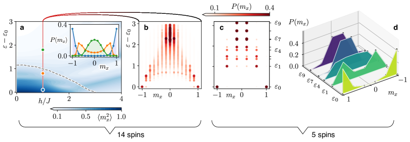
Figure 3: Excited-state phase transition in the Ising model (3) with $\alpha=1.5$. (a) Ferro-paramagnet crossover in the Ising model of $N=14$ spins prepared by the energy measurements in microcanonical ensembles of width $\Delta E/(JN)=0.1$. The transition between magnetically ordered phase $\braket{\hat{m}_{x}^{2}}_{\text{mc}}\approx 1$ (dark blue) to disordered phase $\braket{\hat{m}_{x}^{2}}_{\text{mc}}\approx 0$ (light blue) is shown as function of the mean energy density $\varepsilon=\braket{\hat{H}}_{{\rm mc}}/(JN)$ and the transverse field $h$. An estimate of the critical energy density in the thermodynamic limit, obtained with Monte-Carlo simulation of canonical ensembles of $512$ spins with rescaled interactions (see Methods and Supplementary Note XII), is shown as black dashed line. The inset shows the order parameter distribution $P\left(m_{x}\right)$ for $h/J=1$ and $\varepsilon=0.1,\,0.8,\,1.8$ in blue, orange, and green, respectively. Test of ETH (within the symmetry sector $\left\{+1,-1\right\}$ see Methods): (b) order-disorder transition is seen as crossover from bi-modal distribution of $P\left(m_{x}\right)$ at low energies to a single-peak distribution at high energies, shown on the level individual eigenstates. Color intensity and the dot size indicate the corresponding probability. (c, d) Qualitatively similar energy dependence of $P\left(m_{x}\right)$ shown for a system of just 5 spins. (d) Signatures of the phase transition visible for representative sample of eigenstates.

II.3 QND measurement protocols

Implementation of $\hat{H}_{\mathcal{SM}}$ with time-dependent system-meter coupling $\vartheta(t)$ allows protocols where we switch between time-windows of unobserved quantum simulation, and measurement of energy, and thus preparation of energy eigenstates, which is verified by observing convergence of the filtered photocurrent. In addition, the Hamiltonians (3) and (6) can be made time-dependent, e.g. with a time-dependent magnetic field. This allows us to perform work on the system, and measure work distribution functions via measurement of energy Campisi2011 . Our QND toolbox thus opens up the door to address experimentally fundamental problems of (non-equilibrium) statistical mechanics in analog quantum simulation. We apply the QND toolbox below first to ETH DAlessio2016 ; Deutsch2018 and then we consider testing QFRs Campisi2011 in interacting many-body systems. We emphasize that our setting explores naturally the interesting regime of mesoscopic particle numbers from a few to tens of spins.

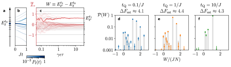
Figure 4: Verification of Jarzynski equality (7) for the transverse field Ising model with 5 spins. A single realisation of the proposed protocol consists of (a) the projection of the initial thermal state of spins to an eigenstate $E_{\ell}^{t_{0}}$ of the initial Hamiltonian with transverse field value $h_{t_{0}}$, (b) the free evolution under a linear change of the transverse field $h$ during time $t_{\rm Q}=t_{1}-t_{0}$ (probabilities $P_{\ell}(t)$ to populate the instantaneous energy eigenstates are shown in shades of blue), (c) the final energy readout $E_{\ell}^{t_{1}}$ of the system at transverse field $h_{t_{1}}$ (photocurrent realizations for simulated experimental runs are shown in red) resulting in the work $W$ (see text) performed during the non-equilibrium process. (d,e,f) The resulting work probability distribution $\mathcal{P}(W)$ for $h_{t_{0}}=2J$, $h_{t_{1}}=0.5J$, $\alpha=2$, $\beta=0.5/J$, and various quench times $t_{\rm Q}$. The gray bars show theoretical probability as a function of work $W$. The color dots with the corresponding vertical error bars (one standard deviation) show the estimated probabilities for 1000 simulated experimental runs. Independent of the quench duration the Jarzynski relation (7) yields similar estimations of the free energy difference $\Delta F_{\rm est}$ (fluctuating due to the finite number of runs) with the true value given by $\Delta F\approx 4.35$.

II.4 Thermal properties of energy eigenstates

Single energy eigenstates $\ket{\ell}$ can encode thermal properties which we typically associate with a microcanonical or canonical ensemble describing systems in thermodynamic equilibrium. This eigenstate thermalization concerns on the one hand expectation values of few-body observables, leading to the remarkable prediction of the ETH that diagonal matrix elements $\braket{\ell}{\hat{O}}{\ell}$ have to agree with the microcanonical average at energy $E_{\ell}$, $\braket{\ell}{\hat{O}}{\ell}=O(E_{\ell})=\mathop{\mathrm{tr}}(\hat{O}\hat{\rho}_{E_{\ell}}^{\mathrm{mc}})$. Here $\hat{\rho}_{E_{\ell}}^{\mathrm{mc}}$ is the microcanonical density operator as a mixture of energy eigenstates within a narrow range centered around $E_{\ell}$. On the other hand, ETH imposes constraints on dynamical properties for diagonal and off-diagonal matrix elements $\braket{\ell^{\prime}}{\hat{O}}{\ell}$; e.g. two-time correlation functions and dynamical susceptibilities have to be related by the fluctuation-dissipation theorem DAlessio2016 . To be more specific, ETH suggests a structure Srednicki1999 $\braket{\ell^{\prime}}{\hat{O}}{\ell}=O(\bar{E})\delta_{\ell^{\prime}\ell}+e^{-S(\bar{E})/2}f_{\hat{O}}(\bar{E},\omega)R_{\ell^{\prime}\ell}$ where diagonal and off-diagonal matrix elements are determined by the functions $O(\bar{E})$ and $f_{\hat{O}}(\bar{E},\omega)$, respectively, which depend smoothly on their arguments $\bar{E}=(E_{\ell}+E_{\ell^{\prime}})/2$ and $\omega=E_{\ell^{\prime}}-E_{\ell}$. $S(\bar{E})$ is the thermodynamic entropy at the mean energy $\bar{E}$, and $R_{\ell^{\prime}\ell}$ is a random number with zero mean and unit variance. An experimental test of ETH, therefore, requires the ability to measure both diagonal and off-diagonal elements, something which is provided by our ion toolbox.

The transverse Ising model (3), as realized with ions, provides a rich testbed for ETH Fratus2016 . For $1<\alpha\leq 2$, this model features a ferromagnetic transition at finite temperature or energy density, in a canonical or microcanonical description, respectively. As illustrated above in Fig. 1, our trapped-ion QND toolbox enables the preparation of microcanonical ensembles of variable width $\Delta E$. According to ETH, the ferromagnetic transition persists even in the limit of vanishing $\Delta E$, which corresponds to the preparation of a single energy eigenstate.

For reference, the microcanonical phase diagram at finite $\Delta E$ is shown in Fig. 3(a) for an experimentally accessible system size of $N=14$ spins and $\alpha=1.5$ (see Supplementary Note XI for experimental parameters). The ferromagnetic transition is clearly manifest in the distribution $P(m_{x})$ of the magnetization $\hat{m}_{x}=N^{-1}\sum_{j}\hat{\sigma}_{j}^{x}$, which is bimodal in the ferromagnetic phase, see the inset in Fig. 3(a). Consequently, fluctuations $\braket{\hat{m}_{x}^{2}}$ are finite (vanish) in the ferromagnetic (paramagnetic) phase, and indicate order even in the absence of symmetry-breaking fields. A trapped-ion quantum simulator provides the ability to perform single-site resolved read-out of spins, thus giving direct access to the distribution $P(m_{x})$ and, consequently, the fluctuations $\braket{\hat{m}_{x}^{2}}$. Due to the quasi-diagonal structure of $\braket{\ell^{\prime}}{\hat{O}}{\ell}$ for ETH-satisfying observables $\hat{O}$, the hypothesis is expected to hold for any power of such observables and, in particular, also for the full probability distribution function $P(m_{x})$ Srednicki1999 . Indeed, as we show in Figs. 3(b) and (c,d), respectively, we find clear signatures of the transition in $P(m_{x})$ for individual energy eigenstates both for $N=14$ and even much smaller system of only $N=5$ spins, in which single eigenenergies can be resolved with current experimental technology (see Supplementary Note XI).

The observation of the Ising transition in single eigenstates gives a qualitative indication of eigenstate thermalization in diagonal matrix elements. A stringent quantitative assessment requires to show that fluctuations of single-eigenstate expectation values $\braket{\ell}{\hat{O}}{\ell}$ around the microcanonical average $\mathop{\mathrm{tr}}(\hat{O}\hat{\rho}_{E_{\ell}}^{\mathrm{mc}})$ are suppressed with increasing system size DAlessio2016 . We discuss experimental requirements for such a test, along with a protocol to measure off-diagonal matrix elements, in Supplementary Note XIII.

II.5 Work distribution function and quantum fluctuation relations

Projective measurements in the energy eigenbasis are the key ingredient for the long-sought experimental verification of QFRs Campisi2011 . The challenging requirement to measure changes in the energy of the system on the level of single energy eigenstates has been achieved only recently in single-particle systems Batalhao2014 ; Zhang2014 . Our QND measurement scheme opens up the possibility to probe QFRs in a true many-body setting.

As an illustration we consider the celebrated Jarzynski equality which describes the mean value of the exponentiated work performed on a system in an arbitrary non-equilibrium process defined by a time-dependent Hamiltonian $\hat{H}(t)$ Campisi2011 . The equality relates the work to the difference between the free energies $\Delta F$ of equilibrium systems described by the Hamiltonian at the initial $t_{0}$ and the final $t_{1}$ times:

$$\left\langle e^{-\beta W}\right\rangle=e^{-\beta\Delta F}.$$ (7)

Here $\beta$ is the inverse temperature specifying an initial canonical thermal state of the system $\hat{\rho}_{\beta}=e^{-\beta\hat{H}(t_{0})}/Z_{t_{0}}$ with $Z_{t_{0}}=\mathop{\mathrm{tr}}[e^{-\beta\hat{H}(t_{0})}]$ and $\Delta F=F_{t_{1}}-F_{t_{0}}=-\ln(Z_{t_{1}}/Z_{t_{0}})/\beta$. The average on the left hand side of Eq. (7) is performed with respect to the distribution of work $\mathcal{P}(W)$ (see Methods). The work itself is determined as the difference between the outcomes of two energy measurements before and after the time-dependent protocol $W\equiv E_{\ell^{\prime}}^{t_{1}}-E_{\ell}^{t_{0}}$. Remarkably, while the work distribution does depend on details of the time evolution given by $\hat{H}(t)$, the average is defined only by the initial and final Hamiltonians. Therefore, the QFR enables experimental measurements of the equilibrium property $\Delta F$ via measurement of work in a non-equilibrium process.

Our scheme provides the required ingredients for probing the QFR in the interesting regime of intermediate system sizes which is dominated by quantum fluctuations: As presented above, the scheme allows for independent temporal control of parameters of the spin Hamiltonian as well as the system-meter coupling in Eq. (2). Further, single energy levels are well resolved for a system of five interacting spins as we consider in the following (see Supplementary Note XI for experimental parameters).

This enables the protocol shown in Fig. 4(a-c), in which a first measurement of the energy is carried out while the magnetic field $h$ in Eq. (3) is kept constant at a value $h_{t_{0}}$. Then, the system-meter coupling is switched off, and the magnetic field is linearly ramped to a final value $h_{t_{1}}$, followed by another measurement. The statistics of corresponding measurement outcomes, $E_{\ell}^{t_{0}}$ and $E_{\ell^{\prime}}^{t_{1}}$, determines the distribution of work $\mathcal{P}(W)$ performed on the system during the magnetic field ramp. Initialization of the system at arbitrary temperatures can be emulated by weighting different runs of the protocol according to the Gibbs distribution $e^{-\beta E_{\ell}^{t_{0}}}/Z_{t_{0}}$ with the initial energy $E_{\ell}^{t_{0}}$.

The resulting work distributions $\mathcal{P}(W)$ for various quench durations $t_{\rm Q}$ are shown in Fig. 4(d-f). While the probability distribution for fast (blue dots) and slow (green dots) quenches differs significantly the estimated free energy difference $\Delta F_{\rm est}=-\ln\langle e^{-\beta W}\rangle/\beta$ approximately (due to the finite number of simulated experimental runs) matches the true value of $\Delta F$ for all three quench speeds, thus, verifying the equality (7).

III Discussion

We have developed a QND toolbox in analog quantum simulation realising single-shot measurement of the energy of an isolated quantum many-body system, as a key element towards experimental studies in non-equilibrium quantum statistical mechanics. This comprises ETH and quantum thermodynamics, including quantum work distribution, and Jarzynski and Crooks fluctuations relations Campisi2011 in mesoscopic quantum many-body systems. The present work outlines an ion-trap implementation with COM phonons as meter. However, the concepts and techniques carry over to other platforms including CQED with atoms RevModPhys.85.553 and superconducting qubits Houck:2012aa , where the role of the meter can be represented by cavity photons read with homodyne detection, and Rydberg tweezer arrays Norcia2018 ; Cooper2018 ; Keesling:2019aa ; Barredo:2018aa ; PhysRevLett.122.143002 by coupling to a small atomic ensemble encoding the continuous meter variables hammerer2010quantum , respectively. Finally, while the present work considers QND measurement of the total Hamiltonian $\hat{H}$ of an isolated system, our approach generalizes to measuring Hamiltonians $\hat{H}_{A}$ of subsystems, as is of interested in quantum transport of energy, or energy exchange in coupling the many-body system of interest to a bath.

IV Methods

IV.1 System-meter coupling Hamiltonian

We choose for the four lasers in our double MS configuration the detuning and the Rabi frequency as $(\Delta,\Omega)$, $(-\Delta,\Omega+\delta\Omega)$, $(\Delta^{\prime},\Omega)$, $(-\Delta^{\prime},\Omega+\delta\Omega)$, where $\delta\Omega\propto\eta^{2}\Omega$ is a small imbalance we use to generate the transverse field term in the spin model. We are interested in the regime of sufficiently large detunings compared to the Rabi frequency $\Omega$, such that single lasers only virtually excite the ions and the phonon modes, $\Omega\ll\Delta^{(\prime)}$, $\eta_{q}\Omega\ll|\Delta^{(\prime)}-\omega_{q}|$, where $\omega_{q}$ is the oscillation frequency of the $q$-th phonon mode and $\eta_{q}\equiv\eta\sqrt{\omega_{0}/\omega_{q}}$. On large timescales $t\gg 1/\Delta^{(\prime)},1/\omega_{0}$, we obtain an effective Hamiltonian $\hat{H}_{{\cal SM}}$ describing the coupled dynamics of the system and the meter, i.e., the spins and the COM phonon mode, by performing the Magnus expansion BLANES2009151 to the time evolution operator in the interaction picture (see Supplementary Note XI). We further expand $\hat{H}_{{\cal SM}}$ in terms of $\eta$. In second order in $\eta$ we recover the transverse field Ising Hamiltonian Zhang2017 ; Britton2012 ; Jurcevic:2014aa , $\hat{H}_{{\cal SM}}^{\left(2\right)}=(-\sum_{i<j}J_{ij}\hat{\sigma}_{i}^{x}\hat{\sigma}_{j}^{x}+h\sum_{j}\hat{\sigma}_{j}^{z})\otimes\mathbb{I}\equiv\hat{H}^{\prime}\otimes\mathbb{I}$, where the spin-spin couplings

$$J_{ij}=-\eta^{2}\omega_{0}\sum_{q}M_{iq}M_{jq}\left[\frac{\Omega^{2}}{\Delta^{2}-\omega_{q}^{2}}+\frac{\Omega^{2}}{(\Delta^{\prime})^{2}-\omega_{q}^{2}}\right]$$ (8)

include contributions from the two MS configurations independently with $M_{iq}$ denoting the distribution matrix element of the $q$-th phonon mode. The transverse field strength is $h=\Omega\delta\Omega\left(1/\Delta+1/\Delta^{\prime}\right)/2$.

Crucially, under the condition $\Delta^{\prime}-\Delta=\omega_{0}$, the crosstalk between the two MS configurations leads to an extra resonant processes as exemplified by Fig. 2(c). These are described by expanding the effective Hamiltonian $\hat{H}_{{\cal SM}}$ to third order in $\eta$, $\hat{H}_{{\cal SM}}^{\left(3\right)}=(-\eta\sqrt{2}M_{i0})(-\sum_{i<j}J_{ij}\hat{\sigma}_{i}^{x}\hat{\sigma}_{j}^{x}-h\sum_{j}\hat{\sigma}_{j}^{z})\otimes\hat{P}\equiv{\vartheta}\hat{H}\otimes\hat{P}$, where $M_{i0}\simeq 1/\sqrt{{N}}$ is the (equal) distribution matrix element of the COM mode. Combining $\hat{H}_{{\cal SM}}^{\left(2\right)}$ and $\hat{H}_{{\cal SM}}^{\left(3\right)}$ gives the desired system-meter Hamiltonian (2). The transverse field in $\hat{H}_{{\cal SM}}^{\left(2\right)}$ and $\hat{H}_{{\cal SM}}^{\left(3\right)}$ can be independently tuned with the method discussed in the main text. Higher order terms beyond $\hat{H}_{{\cal SM}}^{\left(3\right)}$ have negligible effects, for details see Supplementary Note XI.

Our double MS configuration can be implemented with both axial and transverse phonon modes. The implementation with transverse modes gives rise to power-law spin interactions $J_{ij}=J/|i-j|^{\alpha}$ with $0\leq\alpha\leq 3$, which are considered in the rest of this paper. Experimental considerations and scalability are discussed in the Supplementary Note XI.

IV.2 Continuous readout of $\hat{X}$

We assume that in Fig. 2 the ancillary ion does not see the four MS lasers (amber and blue) and, similarly, the system ions do not couple to the read-out laser (red), i.e we assume single-ion addressability Linke3305 or with mixed-species Negnevitsky:2018aa . The read-out laser is tuned in resonance with the red sideband of the COM mode, $\Delta_{\rm e}=\omega_{0}$, under the resolved-sideband condition $\omega_{0}\gg\Gamma_{\rm e},\Omega_{0}$, where $\Gamma_{\rm e}$ is the spontaneous emission rate of the cooling transition $\left|e\right\rangle\to\left|g\right\rangle$ while $\Omega_{0}$ and $\Delta_{\rm e}$ are the Rabi frequency and the detuning of the cooling laser respectively. In this regime, the emitted electric field is proportional to $\langle\hat{a}_{0}\rangle$ with $\hat{a}_{0}$ the annihilation operator of the COM mode. Homodyne detection then directly reveals the quadrature of the COM phonon (the meter). The homodyne current can be written as (see Supplementary Note XI)

$$dX(t)\equiv I(t)dt=\sqrt{2\epsilon\gamma_{\rm s}}\langle\hat{X}\rangle_{\rm c}+dW(t),$$ (9)

where $\epsilon$ is the photon detection efficiency, $\gamma_{\rm s}\simeq k_{0}^{2}\Omega_{0}^{2}/(2\Gamma_{\rm e}Nm_{0}\omega_{0})$ is the measurement rate with $k_{0}$ the cooling laser wavevector and $m_{0}$ the ancillary ion mass, and we have chosen the frequency and phase of the homodyne local oscillator to maximize the homodyne current. Correspondingly, the evolution of the conditional state $\rho_{\rm c}^{\mathcal{SM}}(t)$ of spin system plus the meter is described by a SME

$$d\hat{\rho}_{\rm c}^{\mathcal{SM}}(t)= -i[\hat{H}_{{\cal SM}},\hat{\rho}_{\rm c}^{\mathcal{SM}}(t)]dt+\gamma_{\rm s}\mathcal{D}\left[\hat{a}_{0}\right]\hat{\rho}_{\rm c}^{\mathcal{SM}}(t)dt$$

$$+\sqrt{\epsilon\gamma_{\rm s}}\mathcal{H}\left[\hat{a}_{0}\right]\hat{\rho}_{\rm c}^{\mathcal{SM}}(t)dW(t),$$ (10)

Eliminating the meter under the condition $\gamma_{\rm s}\gg|\vartheta J|$, we realize continuous QND readout of the spin Hamiltonian as described by Eqs. (4) and  (5) with $\gamma=2(\vartheta J)^{2}/\gamma_{\rm s}$.

We further emphasize that the readout laser, which is tuned to the red sideband, also acts as cooling of the COM mode. Furthermore, the readout signal can be enhanced with several ancilla ions.

IV.3 Energy measurement resolution

Here we estimate the Signal-to-Noise Ratio (SNR) which allows us to distinguish two adjacent energy levels separated by $\Delta E$. The difference of photocurrents (5) corresponding to the two energy levels integrated over time $\tau$ reads

$$\int_{0}^{\tau}\!\![I_{1}(t)-I_{2}(t)]dt=\underset{{\rm Signal}}{\underbrace{\vphantom{\int}2\sqrt{\gamma\epsilon}(\Delta E/J)\tau}}+\underset{{\rm Noise}}{\underbrace{\int_{0}^{\tau}\!\![dW_{1}(t)-dW_{2}(t)]}}.$$

Considering the shot noises $W_{1,2}(t)$ of two measurements as uncorrelated and using the Wiener increment property $dW_{1,2}^{2}(t)=dt$ we obtain ${\rm SNR}=2\gamma\epsilon(\Delta E/J)^{2}\tau$. For a given averaging time $\tau$, the condition ${\rm SNR}\gg 1$ provides us with the minimal energy difference we can distinguish $\Delta E/J\gg 1/\sqrt{2\gamma\epsilon\tau}$.

IV.4 Symmetries of the long-range transverse field Ising model

The transverse field Ising model (3) is invariant under the reflection and spin inversion symmetry transformations. We now provide an operational definition of these symmetries and the corresponding symmetry sectors.

Consider a product state vector in the $\sigma^{x}$ basis $\left|\phi\right\rangle=\left|s_{1}^{x}\ldots s_{N}^{x}\right\rangle$. The reflection operator can be defined by its action on the $\left|\phi\right\rangle$ state as $R\left|s_{1}^{x},\ldots,s_{N}^{x}\right\rangle\equiv\left|s_{N}^{x},\ldots,s_{1}^{x}\right\rangle$. Analogously, the spin inversion operator can be defined as $P\left|s_{1}^{x}\ldots s_{N}^{x}\right\rangle\equiv\left|-s_{1}^{x},\ldots,-s_{N}^{x}\right\rangle$. Both operators have two eigenvalues $\pm 1$ and commute with each other and the Hamiltonian Eq. (3), thus, representing QND observables which can also be measured in the non-destructive way as presented in the paper.

The Hamiltonian can be independently diagonalized in each of the subspaces corresponding to eigenvalues of the $R$ and $P$ operators. The ground state of the Ising model with $J,\,h>0$ belongs to the $\left\{+1,+1\right\}$ symmetry sector. For the test of ETH in Fig. 3 we consider the symmetry sector with eigenvalues of $R$ and $P$ given by $\left\{+1,-1\right\}$, respectively. The subspace can be reached from the $\left\{+1,+1\right\}$ sector by flipping odd number of spins (along the $\sigma^{z}$ direction) in the limit of strong transverse field.

IV.5 Interaction renormalization

In numerical simulations in Fig. 3 we renormalize the interaction strength coefficient $J$ such that the average interaction strength matches its value in thermodynamic limit. More precisely, for the $N$-spin Ising model (3) we rescale $J\rightarrow J_{N}\equiv J\cdot S_{N}/S_{\infty}$ with $S_{N}\equiv\frac{1}{N}\sum_{i,j=1}^{N}1/\left|i-j\right|^{\alpha}$. The results are then expressed in units of $J_{14}$.

IV.6 Work distribution function

The work distribution of a process defined by a time-dependent Hamiltonian $\hat{H}(t)$ (with the corresponding instantaneous energy eigenvalues and eigenstates $E_{\ell}^{t}$ and eigenstates $\psi_{\ell}^{t}$ ) is defined as follows Campisi2011 :

$$\mathcal{P}(W)=\sum_{\ell\ell^{\prime}}\delta[W-(E_{\ell^{\prime}}^{t}-E_{\ell}^{0})]P_{\ell^{\prime}\ell}^{t}P_{\ell}^{0},$$ (11)

where $P_{\ell}^{0}=\left\langle\psi_{\ell}^{0}\right|\rho_{{\rm in}}\left|\psi_{\ell}^{0}\right\rangle$ are the occupation probabilities of the initial state and $P_{\ell^{\prime}\ell}^{t}=|\left\langle\psi_{\ell^{\prime}}^{t}\right|U(t,0)\left|\psi_{\ell}^{0}\right\rangle|^{2}$ are the transition probabilities between initial $\ell$ and final $\ell^{\prime}$ states with $U(t,0)\equiv\mathcal{T}e^{-i\int_{0}^{t}\hat{H}(t^{\prime})dt^{\prime}}$ the evolution operator. The average of the exponentiated work in Eq. (7) is readily defined as an integral with the work distribution function Eq. (11): $\langle e^{-\beta W}\rangle\equiv\int dWe^{-\beta W}\mathcal{P}(W)$.

V Data availability

The data sets generated and analyzed in the current study are available from the corresponding author upon reasonable request.

VI Code availability

The codes used to generate the numerical data in the current study are available from the corresponding author upon reasonable request.

VII Acknowledgments

We thank M. Rigol, A. Sørensen, M. Srednicki, and P. Talkner for valuable comments. This work is supported by the European Union’s Horizon 2020 program under Grants Agreement No. 817482 (PASQuanS) and No. 731473 (QuantERA via QTFLAG), the US Air Force Office of Scientific Research (AFOSR) via IOE Grant No. FA9550-19-1-7044 LASCEM, the Austrian Research Promotion Agency (FFG) via QFTE project AutomatiQ, by the Simons Collaboration on Ultra-Quantum Matter, which is a grant from the Simons Foundation (651440, P.Z.). DY acknowledges the financial support by Industriellenvereinigung Tirol. PZ thanks KITP for hospitality as member of the QSIM19 program, and support through Grant NSF PHY-1748958. The stochastic master equation is solved using the open-source QuTiP package JOHANSSON2013 . We use QuSpin for the exact diagonalization of the Ising model Weinberg_17 . For the quantum Monte-Carlo simulations we use the ALPS code Bauer_2011 .

VIII Author contributions

D.Y., A.G., L.M.S., and D.V.V. designed the model, developed the methods, performed the calculations, and analysed the data. All authors discussed the results and wrote the manuscript. P.Z. conceived the study and was in charge of the overall direction and planning.

IX Competing interests

The authors declare no competing interests.

X Additional information

Supplementary information is available for this paper.

Supplementary Information

This Supplementary Information is organized as follows: Supplementary Note XI contains a detailed discussion of the implementation of the QND measurement scheme in a trapped-ion quantum simulator, including an analysis of the experimental feasibility of the scheme with different species of ions and using transverse or axial phonon modes. We provide additional information on applications of the QND scheme in Supplementary Note XII and XIII. In particular, we give details on the numerical analysis of the ferromagnetic transition in the transverse-field Ising, and discuss prospects of an experimental test of the ETH.

XI Implementation with trapped ions

In the main text we outline the implementation of our QND measurement scheme in a trapped-ion quantum simulator. In this section we elaborate on the detailed derivations behind the short presentation in the main text, and discuss the experimental feasibility of the proposed scheme. The section is structured as follows.

In Supplementary Note XI.1 we introduce and provide an analytical study of the double Mølmer-Sørensen (MS) laser configuration (see Fig. 2 of the main text). We show that the low-frequency dynamics is governed by the effective system-meter coupling Hamiltonian $\hat{H}_{{\cal SM}}$, defined in Eq. (2) of the main text (we set $\hbar=1$ hereafter)

$$\hat{H}_{{\cal SM}}=\hat{H}^{\prime}\otimes\mathbb{I}+\vartheta\hat{H}\otimes\hat{P},$$ (12)

where $\hat{P}\equiv i(\hat{a}_{0}^{\dagger}-\hat{a}_{0})/\sqrt{2}$ is the quadrature operator of the center-of-mass (COM) phonon mode, with $\hat{a}_{0}(\hat{a}_{0}^{{\dagger}})$ the corresponding annihilation(creation) operator. Both $\hat{H}$ and $\hat{H}^{\prime}$ are many-body spin Hamiltonians of the Ising type,

$$\hat{H} =-\sum_{i<j}^{N}J_{ij}\hat{\sigma}_{i}^{x}\hat{\sigma}_{j}^{x}-h\sum_{j=1}^{N}\hat{\sigma}_{j}^{z},$$ (13)

$$\hat{H}^{\prime} =-\text{$\sum_{i<j}^{N}J_{ij}\hat{\sigma}_{i}^{x}\hat{\sigma}_{j}^{x}$}-(B-h)\sum_{j=1}^{N}\hat{\sigma}_{j}^{z}.$$ (14)

By adjusting the transverse field strength $B$, we are able to tune the measurement from QND $(B=2h)$ to imperfect QND $(B\simeq 2h)$ which supports the observation of quantum jumps.

In Supplementary Note XI.2 we provide a numerical study of the double MS scheme in different parameter regimes which supports the validity of the system-meter coupling Hamiltonian Eq. (12).

In Supplementary Note XI.3 we describe the continuous readout of the spin Hamiltonian $\hat{H}$, achieved by sideband laser cooling of the motion of an ancilla ion at the edge of the ion chain and homodyne detection of its fluorescence, as schematically shown in Fig. 2(a) of the main text. We derive the resulting dynamics of the spin system as described by the stochastic master equation (SME)

$$d\hat{\rho}_{c}(t) = -i[\hat{{H}}^{\prime},\hat{\rho}_{c}(t)]dt+\gamma\mathcal{D}[\hat{H}/J]\hat{\rho}_{c}(t)dt$$ (15)

$$+\sqrt{\epsilon\gamma}\mathcal{H}[\hat{H}/J]\hat{\rho}_{c}(t)dW(t).$$

Here $\hat{\rho}_{c}(t)$ is the density matrix of the spin system conditioned on the homodyne detection signal, $J$ is the characteristic energy scale of the spin Hamiltonian, $\gamma$ is an effective measurement rate, $\epsilon$ is an overall detection efficiency and $dW(t)$ a white noise Wiener increment. For the detailed expressions of $J$ and $\gamma$, cf. the main text or Supplementary Note XI.3 below. The corresponding homodyne current reads

$$I(t)=2\sqrt{\epsilon\gamma}\langle\hat{H}/J\rangle_{c}+\xi(t),$$ (16)

with $\xi(t)$ white (shot) noise $dW(t)\equiv\xi(t)dt$. We conclude Supplementary Note XI.3 with a brief discussion on the filtering of the homodyne current.

In Supplementary Note XI.4 we discuss some experimental considerations on the proposed trapped-ion implementation, including the analysis of its scalability, and the discussion of its robustness against major experimental imperfections. Supplementary Note XI.4 also provides typical numbers for a proof-of-principle experiment.

We remark that our QND measurement scheme can be implemented with both transverse ($x$ direction) and axial ($z$ direction) phonon modes of the 1D ion string. While transverse phonon modes give rise to the power-law spin interactions $J_{ij}\propto|i-j|^{-\alpha}$ with $1<\alpha<3$ as is considered in the main text, axial phonon modes provide rich opportunities for engineering exotic spin couplings Porras2004 . The derivation of our scheme for both cases is essentially the same. For notational concreteness, in the following Supplementary Notes XI.1 and XI.3, we derive the equations by assuming transverse phonon modes. With the simple replacement $x\to z$ for the ionic motional operators, the same derivation applies to the axial case. In Supplementary Note XI.4, we discuss the features and experimental requirements of the transverse and the axial implementation separately.

XI.1 Analytical study of the double Mølmer-Sørensen configuration

In this section we analyze in detail the laser configuration which generates the desired system-meter coupling $\hat{H}_{{\cal SM}}$ (12) as an effective Hamiltonian derived in perturbation theory for the laser assisted spin-mode couplings. While the model Hamiltonian in the main text refers to the lowest order terms in this expansion, we also derive the higher-order corrections to $\hat{H}_{{\cal SM}}$ and argue that they are indeed negligible under typical experimental conditions.

XI.1.1 Light-ion coupling

We consider $N$ ions trapped in a linear Paul trap. The internal structure of each ion is assumed to be a two level system (TLS), consisting of two qubit states $\left|\downarrow\right\rangle$ and $\left|\uparrow\right\rangle$. The transition $\left|\downarrow\right\rangle\rightarrow\left|\uparrow\right\rangle$ is driven by two pairs of laser beams, such that each pair realizes a Mølmer-Sørensen (MS) configuration, as shown schematically in Fig. 2 of the main text. The lasers which form the first pair, shown as the amber beams, are detuned by $\pm\Delta$ from the qubit transition frequency $\omega_{\uparrow\downarrow}\equiv E_{\uparrow}-E_{\downarrow}$ respectively, and have wave vector projections $\pm k$ along the $x$ direction; The lasers corresponding to the second pair, shown as the blue beams, are detuned by $\pm\Delta^{\prime}$ from $\omega_{\uparrow\downarrow}$, and have wave vector projections $\mp k$ along the $x$ direction. In the frame rotating at $\omega_{\uparrow\downarrow}$, the full Hamiltonian of the internal and motional degrees of freedom (DOFs) of the ion chain reads

$$\hat{H}_{\text{full}}=\hat{H}_{0}+\hat{V}.$$ (17)

Here $\hat{H}_{0}$ is the Hamiltonian of the external motion of the ions (along the $x$ direction), and can be expressed in terms of the collective phonon modes

$$\hat{H}_{0}=\sum_{q}\omega_{q}\hat{a}_{q}^{\dagger}\hat{a}_{q}.$$ (18)

where $\omega_{q}$ and $\hat{a}_{q}$ respectively denote the frequency and the annihilation operator of the mode $q$. Here, the modes are ordered according to their energy. For transverse phonon modes, the COM mode $q=0$ has the highest frequency, and therefore $\omega_{q}>\omega_{q+1}$. The order of modes is reversed for axial phonon modes. The interaction between the ions and the lasers is described by the Hamiltonian

$$\hat{V}= \frac{1}{2}\sum_{j=1}^{N}\hat{\sigma}_{j}^{+}\Big{(}\Omega_{1}e^{-i\Delta t+ik\hat{X}_{j}+i\zeta_{j}^{1}}+\Omega_{2}e^{i\Delta t-ik\hat{X}_{j}+i\zeta_{j}^{2}}$$

$$+\Omega_{3}e^{-i\Delta^{\prime}t-ik\hat{X}_{j}+i\zeta_{j}^{3}}+\Omega_{4}e^{i\Delta^{\prime}t+ik\hat{X}_{j}+i\zeta_{j}^{4}}\Big{)}+{\rm{H.c}.}$$ (19)

Here $\Omega_{m}$ with $m=1,\dotsc,4$ denotes the Rabi frequency of the laser beams, which is assumed to be real and positive for concreteness. The lasers with indices $m=1,2$ correspond to the first MS pair and are shown as amber beams in Fig. 2 of the main text. The blue beams, which correspond to the lasers with indices $m=3,4$, form the second MS pair. For the $j$-th ion, $\hat{\sigma}_{j}^{+}\equiv\left|\uparrow\right\rangle_{j}\left\langle\downarrow\right|$ is its internal raising operator, and $\zeta_{j}^{m}$ is the phase of laser $m$ at its equilibrium position. The operator $\hat{X}_{j}$ describes the small-amplitude displacement from the equilibrium position along the $x$ direction, and can be expressed in terms of the phonon operators as $k\hat{X}_{j}=\sum_{q}\eta_{q}M_{jq}\left(\hat{a}_{q}+\hat{a}_{q}^{\dagger}\right)$, where $M_{jq}$ is the distribution matrix element of mode $q$, and the Lamb-Dicke (LD) parameters are defined as $\eta_{q}=\eta\sqrt{\omega_{0}/\omega_{q}}$, with $\eta=k/\sqrt{2m\omega_{0}}$.

Hereafter we consider the Rabi frequencies of the four laser beams being approximately equal up to a small offset,

$$\Omega_{1} =\Omega_{3}=\Omega,$$

$$\Omega_{2} =\Omega_{4}=\Omega+\delta\Omega.$$ (20)

According to Supplementary Note XI.1.3, the small Rabi frequency mismatch $\delta\Omega$ creates the desired transverse field term of the Ising Hamiltonians (13) and (14), with the transverse field strength $h\propto\delta\Omega$.

A pair of Mølmer-Sørensen laser beams is known to create the Ising spin Hamiltonian Eq. (14) in the off-resonant regime $\Delta^{(\prime)}\gg\Omega$, $|\Delta^{(\prime)}-\omega_{q}|\gg\eta_{q}\Omega$ (see Refs. Kim2009 and the discussion below). In our double MS configuration, however, an additional term describing the QND coupling between the Ising spin Hamiltonian and the COM phonon mode is generated [see the second term of Eq. (12)]. This is achieved by tuning $\Delta^{\prime}=\Delta+\omega_{0}$, i.e., by choosing the beating between the two pairs of MS lasers to match the COM phonon excitation frequency. It leads to a resonant crosstalk between the two MS configurations, which results in the desired QND coupling term.

In the following, we derive Eq. (12) via a Magnus expansion of the time evolution of the ion chain in the interaction picture. We shall first introduce our method, which is a combined Magnus expansion and Lamb-Dicke expansion, in Supplementary Notes XI.1.2 and XI.1.3, respectively, and then work out the detailed expression of Eq. (12) order by order. We summarize the results in Supplementary Note XI.1.6.

XI.1.2 Magnus expansion: effective Hamiltonian

Performing the gauge transformation $\hat{\sigma}_{j}^{+}\to\hat{\sigma}_{j}^{+}\exp\left[\left.-i\left(\zeta_{j}^{1}+\zeta_{j}^{2}\right)\right/2\right]$ and moving into the interaction picture with respect to $\hat{H}_{0}$, Eq. (19) becomes

$$\hat{V}_{I}= \frac{\Omega}{2}\sum_{j=1}^{N}\hat{\sigma}_{j}^{+}\Big{[}e^{-i\Delta t+ik\hat{X}_{j}\left(t\right)+i\varphi_{j}}$$

$$+{\left(1+\frac{\delta\Omega}{\Omega}\right)}e^{i\Delta t-ik\hat{X}_{j}\left(t\right)-i\varphi_{j}}$$

$$+e^{-i\Delta^{\prime}t-ik\hat{X}_{j}\left(t\right)+i(\theta+\varphi_{j}^{\prime})}$$

$$+\left(1+\frac{\delta\Omega}{\Omega}\right)e^{i\Delta^{\prime}t+ik\hat{X}_{j}(t)+i(\theta-\varphi_{j}^{\prime})}\Big{]}+{\rm{H.c}.}$$ (21)

where the time-dependent position operator can be expressed in terms of the phonon modes as $k\hat{X}_{j}\left(t\right)=\sum_{q}\eta_{q}M_{jq}\hat{x}_{q}(t)$ with $\hat{x}_{q}(t)\equiv\hat{a}_{q}{\rm exp}(-i\omega_{q}t)+{\rm H.c.}$, and the relative laser phases are denoted as $\theta=\left(\zeta_{j}^{3}+\zeta_{j}^{4}-\zeta_{j}^{1}-\zeta_{j}^{2}\right)/2,$ $\varphi_{j}=\left(\zeta_{j}^{1}-\zeta_{j}^{2}\right)/2,$ and $\varphi_{j}^{\prime}=\left(\zeta_{j}^{3}-\zeta_{j}^{4}\right)/2$. We note that the phase $\theta$ is independent of the ion index $j$. For the implementation with transverse phonons considered here, this is simply because the laser phase $\zeta_{j}^{m}$ is independent of $j$. For the axial implementation, this is also true, as the position dependencies of the phases of two counter-propagating lasers cancel each other.

We consider the regime where the MS lasers drive the qubit transition and the phonon sidebands off-resonantly, $\Delta^{(\prime)}\gg\Omega$, $|\Delta^{(\prime)}-\omega_{q}|\gg\eta_{q}\Omega$. The evolution operator corresponding to Eq. (21) can be formally written as a Magnus series,

$$\hat{U}(t) \equiv\exp\left[-i\hat{G}(t)\right]=\text{$\mathcal{T}$exp}\left[-i\int_{0}^{t}dt_{1}\hat{V}_{I}\left(t_{1}\right)\right],$$

$$\hat{G}\left(t\right) =\sum_{l=1}^{\infty}\hat{G}_{l}(t).$$ (22)

Correspondingly, it allows us to define an effective Hamiltonian $\hat{H}_{\text{eff}}\equiv\lim_{t\rightarrow\infty}\hat{G}\left(t\right)/t$ which describes the slow dynamics of the ion chain on a time scale much longer than the phononic oscillation period $\sim 1/\omega_{0}$ Kim2009 . The lowest-order terms of the Magnus series are given by

$$\hat{G}_{1}(t)= \int_{0}^{t}dt_{1}\hat{V}_{I}\left(t_{1}\right)dt_{1},$$ (23)

$$\hat{G}_{2}(t)= -\frac{i}{2}\int_{0}^{t}dt_{1}\int_{0}^{t_{1}}dt_{2}\left[\hat{V}_{I}\left(t_{1}\right),\hat{V}_{I}\left(t_{2}\right)\right],$$ (24)

$$\hat{G}_{3}(t)= -\frac{1}{6}\int_{0}^{t}dt_{1}\int_{0}^{t_{1}}dt_{2}\int_{0}^{t_{2}}dt_{3}$$

$$\Big{\{}\left[\hat{V}_{I}\left(t_{1}\right),\left[\hat{V}_{I}\left(t_{2}\right),\hat{V}_{I}\left(t_{3}\right)\right]\right]$$

$$+\left[\left[\hat{V}_{I}\left(t_{1}\right),\hat{V}_{I}\left(t_{2}\right)\right],\hat{V}_{I}\left(t_{3}\right)\right]\Big{\}}.$$ (25)

In the next section we derive $\hat{H}_{{\rm eff}}$ via explicit calculation of $\hat{G}(t)$ in the long-time limit. In this calculation we further perturbatively expand $\hat{V}_{I}$ in terms of the small Lamb-Dicke parameter $\eta\ll 1$. This allows us to construct $\hat{H}_{{\rm eff}}$ order by order as a systematic expansion in $\eta$.

XI.1.3 Expansion with respect to the Lamb-Dicke parameter $\eta$

We now construct the effective Hamiltonian $\hat{H}_{{\rm eff}}$ as an expansion with respect to the Lamb-Dicke parameter, $\hat{H}_{\text{eff}}=\sum_{\ell=0}^{\infty}\hat{H}_{\text{eff}}^{(\ell)}$ with $\hat{H}_{\text{eff}}^{(\ell)}\propto\eta^{\ell}$. In order to do that, we first expand the interaction Hamiltonian Eq. (21) as $\hat{V}_{I}=\sum_{\ell=0}^{\infty}\hat{V}_{I}^{(\ell)}$, with

$$\hat{V}_{I}^{(\ell)}\left(t\right)= \frac{1}{2\times\ell!}\sum_{j=1}^{N}\hat{\sigma}_{j}^{+}\bigg{[}i\sum_{q}\eta_{q}M_{jq}\hat{x}_{q}\left(t\right)\bigg{]}^{\ell}$$

$$\times\bigg{[}{\Omega}e^{-i\Delta t+i\varphi_{j}}+\left(-1\right)^{\ell}(\Omega+\delta\Omega)e^{i\Delta t-i\varphi_{j}}$$

$$+\left(-1\right)^{\ell}\Omega e^{-i\Delta^{\prime}t+i(\theta+\varphi_{j}^{\prime})}$$

$$+(\Omega+\delta\Omega)e^{i\Delta^{\prime}t+i(\theta-\varphi_{j}^{\prime})}\bigg{]}+{\rm{H.c}.}$$ (26)

To simplify the analysis, hereafter we consider $\theta=0$. Moreover, we choose $\varphi_{j+1}-\varphi_{j}=2\pi s,$ $\varphi_{j+1}^{\prime}-\varphi_{j}^{\prime}=-2\pi s$ with $s\in\mathbb{Z}$. For the implementation using transverse phonon modes, this condition is automatically satisfied, with $s=0$. For the implementation using axial phonon modes, this can be achieved by using the central part of an ion chain in a standard Paul trap with nearly uniform spacing $d$ (or alternatively by using ions in equal-distance ion traps Schulz_2008 ; Harlander2011 ; Mehta2014 ; Wilson2014 ) and by choosing an appropriate wavevector $k$ of the MS beams such that $kd=2\pi s$.

XI.1.4 Contributions from $\hat{G}_{1}(t)$

Substituting the expression Eq. (26) into Eq. (24) and taking into account the conditions $|\Delta|\gg\Omega$ and $|\Delta-\omega_{q}|\gg\eta_{q}\Omega$, we immediately see that $\hat{G}_{1}(t)$ does not contribute to $\hat{H}_{\text{eff}}$. Indeed, $\hat{G}_{1}(t)$ describes small-amplitude fast oscillations at frequency $\sim\Delta$, which average to zero in the long-time regime.

XI.1.5 Contributions from $\hat{G}_{2}(t)$ up to $\eta^{3}$: $\hat{H}_{\cal SM}$

Below, we derive the contribution from $\hat{G}_{2}\left(t\right)$ as an expansion in the Lamb-Dicke parameter. In this derivation, we implicitly assume that the small offset of the Rabi frequency [see Eq. (20)] satisfies $\delta\Omega/\Omega\sim O(\eta_{q}^{2})$.

Transverse field terms.

The zeroth-order expansion of $\hat{H}_{{\rm eff}}$ is readily constructed by plugging $\hat{V}_{I}^{(0)}$ into Eq. (24),

$$\hat{H}_{\text{eff}}^{\left(0\right)} =-\frac{i}{2t}\int_{0}^{t}dt_{1}\int_{0}^{t_{1}}dt_{2}\left[\hat{V}_{I}^{\left(0\right)}\left(t_{1}\right),\hat{V}_{I}^{\left(0\right)}\left(t_{2}\right)\right]$$

$$=h\sum_{j=1}^{N}\hat{\sigma}_{j}^{z}.$$ (27)

We note that here and below, we implicitly assume the long-time limit $t\to\infty$. The zeroth-order contribution provides the transverse field term of the quantum Ising Hamiltonian, with the transverse field strength given by

$$h=\frac{\Omega\delta\Omega}{2}\left(\frac{1}{\Delta}+\frac{1}{\Delta^{\prime}}\right).$$ (28)

Similarly, the first-order expansion $\hat{H}_{{\rm eff}}^{(1)}$ is given by

$$\hat{H}_{\text{eff}}^{\left(1\right)} =-\frac{i}{2t}\sum_{\ell+m=1}\int_{0}^{t}dt_{1}\int_{0}^{t_{1}}dt_{2}\left[\hat{V}_{I}^{(\ell)}\left(t_{1}\right),\hat{V}_{I}^{(m)}\left(t_{2}\right)\right]$$

$$=-\vartheta h\sum_{j=1}^{N}\hat{\sigma}_{j}^{z}\otimes\hat{P},$$ (29)

where $\hat{P}\equiv i(\hat{a}_{0}e^{i\varphi}-\hat{a}_{0}^{\dagger}e^{-i\varphi})/\sqrt{2}$ is a quadrature operator of the COM phonon mode, with $\varphi\equiv\varphi_{j}-\varphi_{j}^{\prime}$ an angle dependent on the laser phases, and $\vartheta=-\eta_{0}\sqrt{2}M_{i0}\simeq-\eta_{0}\sqrt{2/N}$ the dimensionless coupling strength. In the following, we absorb the phase $\varphi$ into the definition of $\hat{a}_{0}$, $\hat{a}_{0}e^{i\varphi}\to-\hat{a}_{0}$, thus $\hat{P}=i(\hat{a}_{0}^{{\dagger}}-\hat{a}_{0})/\sqrt{2}$.

Ising terms.

The second order expansion of $\hat{H}_{{\rm eff}}$ can be constructed analogously,

$$\hat{H}_{\text{eff}}^{\left(2\right)} =-\frac{i}{2t}\sum_{\ell+m=2}\int_{0}^{t}dt_{1}\int_{0}^{t_{1}}dt_{2}\left[\hat{V}_{I}^{(\ell)}\left(t_{1}\right),\hat{V}_{I}^{(m)}\left(t_{2}\right)\right]$$

$$=-\sum_{i<j}J_{ij}\hat{\sigma}_{i}^{x}\hat{\sigma}_{j}^{x}.$$ (30)

In this derivation we dropped terms $\sim\eta^{2}\delta\Omega$ under our assumption $\delta\Omega/\Omega\propto\eta^{2}$. We discuss the effect of these higher-order terms in Supplementary Note XI.1.7. Equation (30) describes an Ising spin-spin coupling with coupling strength

$$J_{ij}= -\Omega^{2}\sum_{q}\eta_{q}^{2}\omega_{q}M_{iq}M_{jq}$$

$$\times\left[\frac{1}{\Delta^{2}-\left(\omega_{q}\right)^{2}}+\frac{1}{(\Delta^{\prime})^{2}-\left(\omega_{q}\right)^{2}}\right],$$ (31)

which includes two independent contributions from the two MS laser configuration.

Finally, the third order expansion of $\hat{H}_{{\rm eff}}$ can be calculated in an analogous (though lengthy) way

$$\hat{H}_{\text{eff}}^{\left(3\right)} =-\frac{i}{2t}\sum_{\ell+m=3}\int_{0}^{t}dt_{1}\int_{0}^{t_{1}}dt_{2}\left[\hat{V}_{I}^{(\ell)}\left(t_{1}\right),\hat{V}_{I}^{(m)}\left(t_{2}\right)\right]$$

$$=-\vartheta\Bigg{(}\sum_{i<j}J_{ij}\hat{\sigma}_{i}^{x}\hat{\sigma}_{j}^{x}+\mathcal{E}\Bigg{)}\otimes\hat{P}.$$ (32)

Here, the spin-spin interaction strength $J_{ij}$ is defined in Eq. (31), and $\vartheta$ and $\hat{P}$ are defined below Eq. (29). $\mathcal{E}\equiv\sum_{j}J_{jj}/2$ is a constant driving field for the COM quadrature, which we neglect in the following as it just leads to a constant component in the measured signal. Equation (32) results from a resonant cross-talk between the two MS laser configuration under the condition $\Delta^{\prime}=\Delta+\omega_{z}$, and describes the QND coupling between the spin Hamiltonian and the quadrature of the COM phonon mode.

In deriving Eq. (32), an important assumption we made is that no other phonon mode is resonantly excited except the COM mode up to third order in the Lamb-Dicke parameter. This “single sideband addressibility” is guaranteed by the condition

$$\sum_{q}\frac{\eta^{2}_{q}\Omega^{2}\omega_{q}\eta_{p}}{[\Delta^{(\prime)}]^{2}-\omega_{q}^{2}}\ll|\omega_{p}-\omega_{0}|,\quad\quad\forall p\neq 0.$$ (33)

Equation (33) can be interpreted physically as follows: In our scheme, the excitation of sideband phonons is achieved by simultaneously flipping two spins. The strength for simutaneously flipping spin $i$ and $j$ is given by $J_{ij}$ in Eq. (31). As a result, the sideband addressing strength is $\sim\eta\Omega^{2}\sum_{q}\eta^{2}_{q}\omega_{q}/\{[\Delta^{(\prime)}]^{2}-\omega_{q}^{2}\}$ (we set $M_{iq}=1$ for a worst-scenario analysis), and should be much smaller than the spectral gap between the COM mode and other modes.

In a transverse-phonon implementation, the phonon spectrum gets denser for increasing number of ions. Thus the validity of condition (33) sets a limit on the scalability of our QND scheme. This is analyzed in detail later in Supplementary Note XI.4. Here, we only note that Eq. (33) is much less stringent than the requirement for sideband addressing via laser flipping individual spins, $\eta_{q}\Omega\ll|\omega_{q}-\omega_{0}|,\quad\forall q\neq 0$, as is required, e.g., by the Cirac-Zoller gate or the near-resonant Mølmer-Sørensen gate. This leads to nice scalability of our QND measurement scheme for a given laser power.

Combining Eqs. (27), (29), (30) and (32), the effective Hamiltonian of the ion chain $\hat{H}_{{\rm eff}}$ can be written in the form of $\hat{H}_{\cal SM}$ in Eq. (12), with the identification

$$\hat{H} =-\sum_{i<j}J_{ij}\hat{\sigma}_{i}^{x}\hat{\sigma}_{j}^{x}-h\sum_{j=1}^{N}\hat{\sigma}_{j}^{z},$$

$$\hat{H}^{\prime} =-\text{$\sum_{i<j}J_{ij}\hat{\sigma}_{i}^{x}\hat{\sigma}_{j}^{x}$}+h\sum_{j=1}^{N}\hat{\sigma}_{j}^{z},$$ (34)

$\vartheta\simeq-\eta_{0}\sqrt{2/N}$ and $\hat{P}=i(\hat{a}_{0}^{{\dagger}}-\hat{a}_{0})/\sqrt{2}$.

XI.1.6 Tuning of $\hat{H}_{{\cal SM}}$

Here we describe a method to further tune the transverse field in $\hat{H}$ and $\hat{H}^{\prime}$ [cf. Eq. (34)] independently, thus allowing to reach the QND sweetspot $\hat{H}=\hat{H}^{\prime}$. To this end, we consider the same laser configuration as in Supplementary Note XI.1.1, nevertheless the detunings of the MS lasers are now respectively modified to $B\pm\Delta,$ $B\pm\Delta^{\prime}$, with $B\sim J\ll\Delta,\Delta^{\prime}$. In the frame rotating at frequency $\omega_{\uparrow\downarrow}+B$, we get an additional term $B\sum_{j=1}^{N}\hat{\sigma}_{j}^{z}$ in the Hamiltonian of the laser-driven ion chain $\hat{H}_{\text{full}}$ [cf. Eq. (17)]. Repeating the same derivation as described in Supplementary Notes XI.1.1 and XI.1.3, we recover exactly the same $\hat{H}$ that is coupled to the meter DOFs, while $H^{\prime}$ is modified as

$$H^{\prime}=\text{$\sum_{i<j}J_{ij}\hat{\sigma}_{i}^{x}\hat{\sigma}_{j}^{x}$}-\left(h-B\right)\sum_{j}\hat{\sigma}_{j}^{z}.$$

By choosing $B=2h$ we realize the QND condition $\hat{H}^{\prime}=\hat{H}$, while offsetting $B$ slightly from $2h$ allows us to observe quantum jumps between different eigenstates of $\hat{H}$.

XI.1.7 Contributions from $\hat{G}_{2}(t)$ beyond $\eta^{3}$: higher-order corrections

In this section we derive the corrections to the QND Hamiltonian Eq. (12) resulting from higher-order terms in the Lamb-Dicke expansion of $\hat{G}_{2}(t)$. We show that these terms do not change the QND character of the proposed measurement scheme.

By straight forward calculation, we find that the fourth order expansion of the effective Hamiltonian can be written as

$$\hat{H}_{\text{eff}}^{\left(4\right)} =-\frac{i}{2t}\sum_{\ell+m=4}\int_{0}^{t}dt_{1}\int_{0}^{t_{1}}dt_{2}\left[\hat{V}_{I}^{(\ell)}\left(t_{1}\right),\hat{V}_{I}^{(m)}\left(t_{2}\right)\right]$$

$$=-\sum_{i<j}J_{ij}^{(4)}\hat{\sigma}_{i}^{x}\hat{\sigma}_{j}^{x},$$ (35)

with the spin-spin coupling

$$J_{ij}^{(4)}= -\frac{\Omega^{2}}{2}\sum_{qp}\eta_{q}^{2}\eta_{p}^{2}M_{iq}M_{jq}M_{ip}M_{jp}(\omega_{q}+\omega_{p})$$

$$\times\left[\frac{1}{\Delta^{2}-(\omega_{q}+\omega_{p})^{2}}+\frac{1}{(\Delta^{\prime})^{2}-(\omega_{q}+\omega_{p})^{2}}\right]$$

$$+\frac{\Omega^{2}}{2}\eta_{0}^{2}\omega_{z}\sum_{p}\eta_{p}^{2}(M_{ip}^{2}+M_{jp}^{2})$$

$$\times\sum_{q}M_{iq}M_{jq}\left[\frac{1}{\Delta^{2}-\omega_{q}^{2}}+\frac{1}{(\Delta^{\prime})^{2}-\omega_{q}^{2}}\right].$$ (36)

In the derivation of Eq. (35), we dropped terms proportional to the phonon-occupation under the assumption $\langle\hat{a}_{q}^{{\dagger}}\hat{a}_{q}\rangle\ll 1$.

Besides $\hat{H}_{\text{eff}}^{\left(4\right)}$, another correction to the QND Hamiltonian that is fourth order in $\eta$ comes from the term $\sim\eta^{2}\delta\Omega\propto\eta^{4}$ which we dropped in Eq. (30). Via straightforward calculation we find this term can be written as a transverse field Ising Hamiltonian with site-dependent transverse field,

$$-\sum_{i<j}t_{ij}\hat{\sigma}_{i}^{x}\hat{\sigma}_{j}^{x}-\sum_{j}\lambda_{j}\hat{\sigma}_{j}^{z},$$ (37)

with the coefficients

$$t_{ij}= -\Omega\delta\Omega\sum_{q}\omega_{q}\eta_{q}^{2}M_{iq}M_{jq}$$

$$\times\left[\frac{1}{\Delta^{2}-\omega_{q}^{2}}+\frac{1}{(\Delta^{\prime})^{2}-\omega_{q}^{2}}\right],$$

$$\lambda_{j}= -2\Omega\delta\Omega\sum_{q}\eta_{q}^{2}M_{jq}^{2}\left(\frac{1}{\Delta}+\frac{1}{\Delta^{\prime}}\right).$$ (38)

Importantly, the corrections to the QND Hamiltonian up to fourth order in the Lamb-Dicke parameter, Eq. (35) and (37), only involve spin DOFs and do not involve phonon DOFs. Thus, they only slightly renormalize the coefficients of $\hat{H}^{\prime}$ [cf. Eq. (34)], introducing tiny mismatch between $\hat{H}^{\prime}$ and $\hat{H}$. As described in the main text, these mismatch only introduce rare quantum jumps between energy eigenstates [cf. Fig. 1(3) of the main text], whereas the QND character of the measurement is maintained.

XI.1.8 Effects of higher order Magnus series

In this section, we show that the contributions to the effective Hamiltonian from higher-order terms in the Magnus series, $\hat{G}_{n}(t),n\geq 3$, are of higher order than $\eta^{4}$. Thus they are much smaller than the system-meter coupling $\hat{H}_{\cal SM}$ and do not change the QND character of the proposed measurement scheme. The following analysis is based on power counting and physical arguments.

Let us first consider the contributions from $\hat{G}_{3}(t)$, cf. Eq. (25). For simplicity, we temporarily assume balanced MS configurations, i.e., $\delta\Omega=0$. In this case, the spin operators $\hat{\sigma}_{j}^{\pm}$ in Eq. (26) can be combined to $\hat{\sigma}_{j}^{x}$. Therefore, spin operators always commute with each other at different time. As a result, the double commutator in the integrand of Eq. (25) is nonzero only if both the inner and outer commutators contain at least a pair of phonon annihilation and creation operators. Such an integrand, contains at least four phonon operators, and its contribution is $O(\eta^{4})$ after the integration. Moreover, it is straightforward to see such a contribution contains a fast oscillating phase $\sim\Delta^{(\prime)}t$ and do not contribute to the effective Hamiltonian. Physically, it corresponds to processes which involve two virtual phonon excitations, which are nevertheless off-resonant. Thus, $\hat{G}_{3}(t)$ contributes $O(\eta^{5})$ to the effective Hamiltonian when $\delta\Omega=0$.

We now reintroduce the imbalance $\delta\Omega$. Keeping in mind that $\delta\Omega/\Omega\sim O(\eta^{2})$, in the integrand of Eq. (26) we can restrict ourselves to ‘relevant’ terms that contain $\delta\Omega$ and at most two phonon operators, since the other terms contribute at $O(\eta^{5})$ after multiplication with $\delta\Omega$. Under the conditions $\Delta^{(\prime)}\gg\Omega$ and $|\Delta^{(\prime)}-\omega_{q}|\gg\eta_{q}\Omega$, which are met in our off-resonant double MS configuration, it is straightforward to verify that the ‘relevant’ terms involving zero or one phonon operator contain fast oscillating phase $\sim\omega_{z}t$ and average to zero in the long time limit. The analysis of the terms consisting of $\delta\Omega$ and two phonon operators is more involved. First, we note that these terms are of the order $O(\eta^{4})$, i.e., much smaller than the QND coupling Hamiltonian $\hat{H}_{\cal SM}$. Secondly, we find that they are off-resonant and average to zero if we avoid ‘accidental’ resonances, by requiring $|\omega_{q}-\omega_{p}|\neq|\Delta-\omega_{0}|,\,\forall p,q$, which can be achieved by choosing appropriate $\Delta$ in experiments. To summarize, the contribution of $\hat{G}_{3}(t)$ can be made as small as $O(\eta^{5})$ and is thus negligible.

Next, we consider the contributions from $\hat{G}_{4}(t)$. Adopting similar arguments as above, we find that if $\delta\Omega=0$ the contribution from $\hat{G}_{4}(t)$ is on the order of $O(\eta^{6})$, and corresponds physically to processes involving three virtual phonon excitations. Reintroducing $\delta\Omega$ and looking at ‘relevant’ terms that contain at most two phonon operators, we find only one term that does not oscillate and remains finite in the long-time limit, under the assumption that accidental resonances are avoided and the phonon occupations are small, $\langle\hat{a}_{q}^{{\dagger}}\hat{a}_{q}\rangle\ll 1$. This term is proportional to $\delta\Omega\times\Omega^{3}/\Delta^{3}\sum_{j}\hat{\sigma}_{j}^{z}$ and describes the AC-Stark shift from fourth-order perturbation theory. Comparing this term to the QND coupling terms (29) and (32), we find it has a relative strength $\Omega^{2}/(\eta\Delta^{2})$. To ensure that this term has negligible effect on the performance of our QND scheme, we thus require $\Omega^{2}/(\eta\Delta^{2})\ll 1$. This is typically true, as $\eta$ and $\Omega/\Delta$ are small parameters which have similar magnitudes.

Along the same lines, we can show that the contributions from $\hat{G}_{n},n>4$ are all negligible.

XI.2 Numerical study of the double Mølmer-Sørensen configuration

We complement the analytical investigation of the double Mølmer-Sørensen laser configuration scheme above by a numerical study of the evolution of a system of $N=3$ ions in a truncated phonon basis, and we identify parameter regimes in which a description of the system in terms of the effective Hamiltonian Eq. (12) is valid. We consider two scenarios: First, we study the evolution with $\delta\Omega=0$, which corresponds to the Ising model with no transverse field $h=0$, and we assume that the QND scheme is implemented with transverse phonon modes. Under these conditions, we show that in a wide range of detunings $\Delta$ the exact dynamics of the joint system consisting of spin and phonon degrees of freedom modes is well reproduced by the effective Hamiltonian Eq. (12). Second, for a fixed value of the detuning $\Delta$, we show that the effective Hamiltonian remains valid for a range of values of the transverse field $h$. This analysis assumes the use of axial phonon modes and is based on Floquet theory.

XI.2.1 Dynamics of phonon modes

The starting point of our consideration is the full Hamiltonian of the system Eq. (21). We focus on the transverse phonon modes and analyse the tunability of the detuning $\Delta$ which defines the spin-spin interaction parameter $\alpha$ as discussed. We assume all Rabi frequencies to be equal ($\delta\Omega=0$), which corresponds to the Ising model with no transverse field Eq. (28). In this case the full Hamiltonian simplifies to:

$$\hat{V}_{I}=\sum_{j=1}^{N}\sigma^{x}_{j}\Big{[}\cos\Big{(}\Delta t-k\hat{X}_{j}(t)\Big{)}+\cos\Big{(}\Delta^{\prime}t+k\hat{X}_{j}(t)\Big{)}\Big{]}.$$ (39)

This implies that for an initial product state in the $\sigma^{x}$ basis there is no dynamics of spin variables, and only the phonon modes evolve in time. If they are initially prepared in their vacuum states then, according to the effective Hamiltonian given in Eqs. (12) and (13), at some final time $t_{f}$ we expect $\langle\hat{x}_{q}\rangle\propto\sqrt{\langle a_{q}^{{\dagger}}a_{q}\rangle}\propto\delta_{q,0}(\sum J_{ij}s^{x}_{i}s^{x}_{j})\cdot t_{f}$, where $\{s^{x}_{i}\}$ denote the initial spin configuration.

To check the validity of our model we compute the mean phonon number $\langle a_{q}^{{\dagger}}a_{q}\rangle$ using the full Hamiltonian Eq. (39) for the corresponding initial spin states as a function of the detuning $\Delta$, while keeping $\Delta^{\prime}=\Delta+\omega_{0}$. The result is shown in Supplementary Fig. 5(a). We observe the appearance of resonances at certain values of $\Delta$, where the evolution does not correspond to the effective Hamiltonian Eq. (12). Partially this can be explained by the poles of the fourth order expansion term of the $J_{ij}$ matrix Eq. (36). The rest of resonances have lower amplitude and higher frequency and we attribute them to the many-phonon resonant processes which correspond to the higher-than-fourth order $\eta$-expansion terms.

Remarkably, there exist wide regions of detuning $\Delta$ free of resonances provided that there is space between the higher order harmonics of the phononic eigenfrequencies $\omega_{0}\gg|\omega_{0}-\omega_{q}|,\,\forall q$. As shown in Supplementary Fig. 5(b) the system dynamics in these regions is well reproduced by the effective model Eqs. (12), (31) such that the COM mode population reflects the eigenenergies of the spin system.

In order to show that the scheme scales well with the number of ions we present in Supplementary Fig. 6(a,b) results for $N=6$ ions interacting via 6 phonon modes. One can see that effective QND dynamics represents the exact results as expected.

The setup which is described in this section is also of interest as a first proof-of-principle experimental test of the proposed QND coupling of the spin model to the COM phonons $\vartheta\hat{H}\otimes\hat{P}$. Importantly, it does not require implementation of the full QND scheme with the continuous readout as the mean phonon-number measurement can be done in a multi-shot fashion.

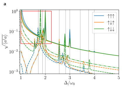
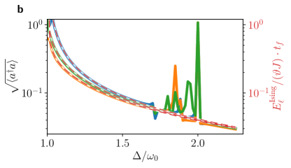
Figure 5: (a) Transverse phonon mode occupation at the final time $t_{f}=2\pi\times 600/\omega_{0}$ for different initial states of $N=3$ spins indicated with blue, green, and orange colors. Solid, dot-dashed and dashed curves stand for the $q=0,1,2$ modes, respectively. Vertical lines represent frequencies of the higher-order harmonics of the phonon modes. (b) Zoomed-in part [red rectangle in (a)] including the first resonances. Dashed curves show the analytical results obtained from Eqs. (12), (31). The numerical parameters: $\eta=0.1$, $\Omega/\omega_{0}=1/6,\omega_{0}/\omega_{z}=3$, the phonon modes are described by 5 Fock states.

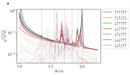
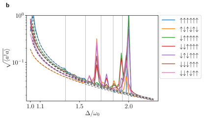
Figure 6: (a) Transverse phonon mode occupation at the final time $t_{f}=2\pi\times 400/\omega_{0}$ for different initial states of $N=6$ spins indicated with various colors. Solid curves stand for the COM mode ($q=0$) population, dashed curves represent the rest of the modes $q\neq 0$. Vertical lines represent frequencies of the higher-order harmonics of the phonon modes. (b) Comparison with the analytical results. Dashed curves show the analytical results obtained from Eqs. (12), (31). Parameters: $\eta=0.1$, $\Omega/\omega_{0}=1/8,\omega_{0}/\omega_{z}=4$. The phonon modes are described by 3 Fock states.

XI.2.2 Floquet spectrum analysis

Here we verify the effective QND dynamics for various transverse field values. In particular, we perform a numerical simulation of the periodically driven system of $N=3$ ions interacting via 3 axial phonon modes according to the full Hamiltonian $\hat{H}_{{\rm full}}(t)$ given by Eq. (17). We choose commensurate detunings $\Delta=-7\omega_{0}$, $\Delta^{\prime}=-6\omega_{0}$, such that the overall dynamics is periodic with frequency $\omega_{0}$. Next, the operator of unitary evolution $\hat{U}(t)=\mathcal{T}\exp\left[-i\int_{0}^{t}dt_{1}\hat{H}_{{\rm full}}(t_{1})\right]$ is numerically evaluated for one period of the oscillation. The logarithm of eigenvalues of $\hat{U}(2\pi/\omega_{0})$ provides $E_{\ell}^{{\rm Floquet}}$ the quasi energies of the effective Hamiltonian.

In Supplementary Fig. 7(a) we compare the Floquet quasi energies $E_{\ell}^{{\rm Floquet}}$ (blue dotted lines) with the spectrum $E_{\ell}^{{\rm Ising}}$ of the effective Ising Hamiltonian (14) with adjusted transverse field $B=2h$ (dashed lines) for various values of the Rabi frequency mismatch $\delta\Omega$ expressed as a transverse field $h$ via Eq. (28). The figure clearly shows that the exact eigenvalues $E_{\ell}^{{\rm Floquet}}$ are well represented by the effective Ising model.

Next, we study the coupling of the Ising Hamiltonian to the COM phonon mode. Here we consider the non-hermitian Hamiltonian of the full system (ions+phonons) $\hat{H}_{{\rm full}}(t)-i\frac{\gamma_{s}}{2}a_{0}^{\dagger}a_{0}$ with the non-hermitian term describing the decay of the COM mode due to the read-out. The Floquet eigenstates with the quasi energies around 0 and small imaginary parts represent the steady states of the open system. The COM mode displacements $\braket{a_{0}+a_{0}^{\dagger}}$ averaged over these Floquet states are shown in Supplementary Fig. 7(b) with red lines. The displacement is proportional to the corresponding eigenenergy of the Ising Hamiltonian (13) shown with dashed lines. The resulting read-out photocurrent is sensitive to the amplitude of the COM mode oscillations and, therefore, reveals the eigenenergies of the desired Ising model.

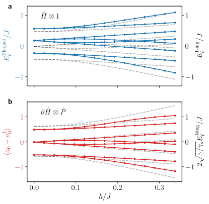
Figure 7: Numerical verification of the double Mølmer-Sørensen configuration via Floquet analysis. (a) Test of the free evolution term $\hat{H}\otimes\mathbb{{I}}$ of the effective system-meter Hamiltonian (12). Blue lines show the exact Floquet spectrum depending on the effective transverse field $h$ (see text), dashed lines represent eigenenergies of the effective Ising model. (b) The system-meter coupling $\vartheta\hat{H}\otimes\hat{P}$ test. Red lines show the COM mode displacement $\braket{a_{0}+a_{0}^{\dagger}}$ averaged over the exact Floquet eigenstates (see text), dashed lines represent the corresponding eigenenergies of the effective Ising model. The following parameters are used: $\eta=0.3$, $\Delta=-7\omega_{0}$, $\Delta^{\prime}=-6\omega_{0}$, $\Omega=\omega_{0}$, $0<\frac{\delta\Omega}{\Omega}<2\times 10^{-3}$, $\gamma_{s}=3\frac{\eta J}{\sqrt{N}}\left(\frac{\eta\Omega}{\Delta}\right)^{2}$. The COM mode is described by 6 Fock states, the other modes use 3 Fock states.

XI.3 Continuous readout of the spin Hamiltonian

With the implementation of the system-meter coupling Hamiltonian Eq. (12) at hand, in this section we present the detailed discussion on the readout of the transverse Ising Hamiltonian via continuous monitoring the center-of-mass phonon quadrature $\hat{X}$, extending the short description presented in the Method section of the main text.

The experimental setup we have in mind is shown schematically in Fig. 2 of the main text. Here, aside from the ions $j\in\{1,\dotsc,N\}$ which generates the QND Hamiltonian Eq. (12), an ancilla ion $j=0$ is trapped at the edge of the ion chain and is subjected to sideband resolved laser cooling. The fluorescence emitted by the ancilla ion is collected by a lens setup and is continuously detected by a homodyne apparatus. We assume the MS lasers doesn’t interact with the ancilla ion, nor does the cooling laser impact the ions $j\in\{1,\dotsc,N\}$. As such, the ancilla ion participates in the collective vibrations of the ion chain and serves as a ‘transducer’ to couple light and phonons, thus allowing for monitoring the latter.

In the following, we introduce the quantum optical model for our considered setup in Supplementary Note XI.3.1, using the language of a quantum stochastic Schrödinger equation (QSSE) (see, e.g., Chap. 9 in Ref. gardiner2015quantum for an introduction). Based on it, in Supplementary Note XI.3.2 we derive a QSSE describing the coupling between the phonons and light by adiabatically eliminating the internal DOFs of the ancilla ion. Finally, in Supplementary Note XI.3.3 we derive the stochastic master equation for continuous homodyne detection of the spontaneously emitted light and arrive at Eqs. (15) and (16).

XI.3.1 Quantum stochastic Schrödinger equation

To be specific, we consider a standing-wave cooling configuration, i.e., the ancilla ion locates at the node of the standing wave cirac1992 . In the interaction picture with respect to $\hat{H}_{0}$ [c.f. Eq. (18)], and in the frame rotating with the frequency of the cooling laser $\omega_{L}$, the internal dynamics of the auxiliary ion is described by

$$\hat{H}_{\text{TLS}}=-\Delta_{e}|e\rangle\langle e|+\frac{\Omega_{0}}{2}(|e\rangle\langle g|+{\rm H.c.})\sin[k_{0}\hat{X}_{0}(t)].$$ (40)

Here, $|g\rangle(|e\rangle)$ is the ground(excited) level of the cooling transition respectively and $\Delta_{e}=\omega_{L}-\omega_{eg}$ is the frequency detuning between the cooling laser and the $|g\rangle\to|e\rangle$ transition. We assume the cooling laser is along the $x$ axis, with wavevector $k_{0}$ and Rabi frequency $\Omega_{0}$. The operator $\hat{X}_{0}(t)$ describes the (small-amplitude) displacement of the ancilla ion around its equilibrium position, and is related to the collective phonon modes of the ion chain by $\hat{X}_{0}(t)=\sum_{q}M_{0q}[\hat{a}_{q}(t)+\hat{a}_{q}^{\dagger}(t)]/\sqrt{2m_{0}\omega_{q}}$ with $m_{0}$ the mass of the ancilla ion, and $\hat{a}_{q}(t)=\hat{a}_{q}{\rm exp}(-i\omega_{q}t)$.

Besides the internal structure of the ancilla ion, the rest DOFs of our model includes the internal pseudo-spins of ion $j\in\{1,\dotsc,N\}$ and the $N+1$ axial phonon modes. In the interaction picture with respect to $\hat{H}_{0}$, the time evolution of the total system is described by the (Itô) QSSE gardiner2015quantum for the ions and the external electromagnetic field (bath DOFs),

$$d|\Psi\rangle= -i\left(\hat{H}_{\cal{SM}}+\hat{H}_{\text{TLS}}-\frac{i}{2}\Gamma_{e}|e\rangle\langle e|\right)|\Psi\rangle dt$$

$$+\int du\sqrt{\Gamma_{e}N(u)}|g\rangle\langle e|e^{-ik_{0}u\hat{X}_{0}(t)}d\hat{B}^{\dagger}(u,t)|\Psi\rangle.$$ (41)

In Eq. (41), the first line includes the spin-phonon Hamiltonian $\hat{H}_{{\rm sys}}$, the internal Hamiltonian of the ancilla ion $\hat{H}_{{\rm TLS}}$, and the spontaneous decay of the ancilla ion at a rate $\Gamma_{e}$. The second line describes spontaneous emission of the ancilla ion into the 3D electromagnetic modes. Here, the function $N(u)$ reflects the dipole emission pattern of the cooling transition, which, for the 1D ionic motion considered here, depends on a single variable $u\equiv\cos\nu\in[-1,1]$ with $\nu$ the angle between the wavevector of the emitted photon and the $x$ axis. The spontaneous emission is accompanied by the momentum recoil described by the operator $e^{-ik_{0}u\hat{X}_{0}}$, with $k_{0}$ the wavevector of the emitted photon (approximately the same as the wavevector of the cooling laser). To account for the relevant electromagnetic modes in the emission direction $u$, quantum optics introduces the corresponding bosonic noise operators $\hat{b}_{u}(t)$ and $\hat{b}_{u}^{{\dagger}}(t)$, satisfying the white-noise commutation relations $[\hat{b}_{u}(t),\hat{b}_{u}^{{\dagger}}(t^{\prime})]=\delta(u-u^{\prime})\delta({t-t^{\prime}})$ gardiner2015quantum . In the Itô QSSE (41) these noise operators are transcribed as Wiener operator noise increments, $\hat{b}_{u}(t)dt\to d\hat{B}(u,t)$. Assuming the 3D bath is initially in the vacuum state, they obey the Itô table gardiner2015quantum ,

$$\begin{split}d\hat{B}(u,t)d\hat{B}^{{\dagger}}(u^{\prime},t)&=dt\delta(u-u^{\prime}),\\ d\hat{B}^{{\dagger}}(u,t)d\hat{B}(u^{\prime},t)&=0,\\ d\hat{B}(u,t)d\hat{B}(u^{\prime},t)&=d\hat{B}^{{\dagger}}(u,t)d\hat{B}^{{\dagger}}(u^{\prime},t)=0.\end{split}$$ (42)

We note, apart from the explicit ion-bath coupling in the second line of Eq. (41), the inclusion of the 3D electromagnetic field bath also introduces a decay term $-i\Gamma_{e}|e\rangle\langle e|/2$ in the first line of Eq. (41). Mathematically, this non-Hermitian term appears as an “Itô correction” when applying the Itô stochastic calculus to describe physical systems gardiner2015quantum .

Based on Eq. (41), in the next section we derive a QSSE describing the coupling between the phonon modes and the electromagnetic field bath by adiabatically eliminating the internal dynamics of the ancilla ion.

XI.3.2 Adiabatic elimination of the internal dynamics of the ancilla ion

We consider the following parameter regime. (i) The ancilla ion is weakly excited by the cooling laser, $\eta_{q}^{0}\Omega_{0}\ll\Gamma_{e}$, where $\eta_{q}^{0}\equiv k_{0}/\sqrt{2m_{0}\omega_{q}}$ is the Lamb-Dicke parameter corresponding to the cooling laser. (ii) The QND interaction is much weaker than the spontaneous emission strength of the ancilla ion, $|\hat{H}_{{\cal SM}}|\ll\Gamma_{e}$. (iii) The sideband resolved regime $\omega_{q}\gg\Gamma_{e}$. Condition (i) and (ii) guarantees that the internal dynamics of the ancilla ion is much faster than the dynamics of the rest of the system, allowing us to adiabatically eliminate the internal dynamics of the ancilla ion. Condition (iii) enables us to selectively enhance the center-of-mass phonon contribution in the detected photon current (see detailed discussion in Supplementary Note XI.3.3).

To perform the adiabatic elimination, we formally decompose the state of the total system [see Eq. (41)] into two components, $|\Psi\rangle=|\psi_{e}\rangle|e\rangle+|\psi_{g}\rangle|g\rangle$, with $|\psi_{e(g)}\rangle\equiv\langle e(g)|\Psi\rangle$. By the expansion up to second order in the small Lamb-Dicke parameter $\eta_{q}^{0}$, Eq. (41) becomes two coupled equations for $|\psi_{e(g)}\rangle$,

$$d|\psi_{e}\rangle= -i\left[\hat{H}_{{\cal SM}}-\left(\Delta_{e}+\frac{i}{2}\Gamma_{e}\right)\right]|\psi_{e}\rangle dt$$

$$-i\frac{\Omega_{0}}{2}\sum_{q}\eta_{q}^{0}M_{0q}\left[\hat{a}_{q}^{\dagger}(t)+\hat{a}_{q}(t)\right]|\psi_{g}\rangle dt,$$ (43)

$$d|\psi_{g}\rangle= -i\hat{H}_{\cal SM}|\psi_{g}\rangle dt-i\frac{\Omega_{0}}{2}\sum_{q}\eta_{q}^{0}M_{0q}\left[\hat{a}_{q}^{\dagger}(t)+\hat{a}_{q}(t)\right]|\psi_{e}\rangle dt$$

$$+\int du\sqrt{\Gamma_{e}N(u)}\bigg{\{}1-i\sum_{q}\eta_{q}^{0}M_{0q}\left[\hat{a}_{q}^{\dagger}(t)+\hat{a}_{q}(t)\right]$$

$$-\frac{1}{2}\Big{[}\sum_{q}\eta_{q}^{0}M_{0q}\left[\hat{a}_{q}^{\dagger}(t)+\hat{a}_{q}(t)\right]\Big{]}^{2}\bigg{\}}d\hat{B}^{\dagger}(u,t)|\psi_{e}\rangle.$$ (44)

From Eq. (43) it is easy to see $|{\psi}_{e}\rangle\sim O(\eta_{q}^{0})$. To keep $|\psi_{g}\rangle$ accurate to $O[(\eta_{q}^{0})^{2}]$, we can neglect the second order Taylor expansion in the last term of Eq. (44).

Under conditions (i) and (ii) introduced in the beginning of this section, Eq. (43) can be solved adiabatically

$$|{\psi}_{e}\rangle=\frac{\Omega_{0}}{2}\sum_{q}\eta_{q}^{0}M_{0q}\bigg{[}\frac{\hat{a}_{q}^{\dagger}(t)}{\Delta_{e}\!-\!\omega_{q}\!+\!\frac{i}{2}\Gamma_{\!e}}\!+\!\frac{\hat{a}_{q}(t)}{\Delta_{e}\!+\!\omega_{q}\!+\!\frac{i}{2}\Gamma_{\!e}}\bigg{]}|{\psi}_{g}\rangle.$$

Plugging the solution into Eq. (44), we arrive at a QSSE which describes the slow dynamics of the system assuming the ancilla ion staying in its internal stationary (ground) state,

$$d|\psi_{g}\rangle= -i\left(\hat{{H}}_{{\cal SM}}+\sum_{q}\delta{\omega}_{q}\hat{a}_{q}^{\dagger}\hat{a}_{q}\right)|\psi_{g}\rangle dt$$

$$-\frac{1}{2}\left(A_{q}^{+}\hat{a}_{q}\hat{a}_{q}^{\dagger}+A_{q}^{-}\hat{a}_{q}^{\dagger}\hat{a}_{q}\right)|\psi_{g}\rangle dt$$

$$+\int du\sqrt{\Gamma_{e}N(u)}\hat{{\cal J}}d\hat{B}^{\dagger}(u,t)|\psi_{g}\rangle,$$ (45)

where $dt\gg 1/\Gamma_{e}$ is the coarse-grained time increment and $d\hat{B}^{{\dagger}}(u,t)$ is the corresponding coarse-grained quantum noise increment. $\delta\omega_{q}$ is a (tiny) frequency renormalization of the $q$-th phonon mode,

$$\delta\omega_{q}=(\eta_{q}^{0}M_{0q}\Omega_{0})^{2}\bigg{[}\frac{\Delta_{e}+\omega_{q}}{4(\Delta_{e}\!+\!\omega_{q})^{2}\!+\!\Gamma_{e}^{2}}+\frac{\Delta_{e}-\omega_{q}}{4(\Delta_{e}\!-\!\omega_{q})^{2}\!+\!\Gamma_{e}^{2}}\bigg{]}.$$

In the following we neglect such a tiny frequency shift. The damping rates $A_{q}^{\pm}$ for the $q$-th phonon mode are defined as

$$A_{q}^{\pm}=\frac{(\eta_{q}^{0}M_{0q}\Omega_{0})^{2}}{4(\Delta_{e}\mp\omega_{q})^{2}+\Gamma_{e}^{2}}\Gamma_{e}.$$ (46)

The operator $\hat{{\cal J}}$ is a collective quantum jump operator including all phonon modes,

$$\hat{{\cal J}}=\frac{\Omega_{0}}{2}\sum_{q}\eta_{q}^{0}M_{0q}\bigg{(}\frac{\hat{a}_{q}^{\dagger}(t)}{\Delta_{e}-\omega_{q}+\frac{i}{2}\Gamma_{e}}+\frac{\hat{a}_{q}(t)}{\Delta_{e}+\omega_{q}+\frac{i}{2}\Gamma_{e}}\bigg{)}.$$ (47)

The QSSE (45) describes the coupling between the phonon DOFs and the external electromagnetic field bath. This allows us to read out the COM quadrature $\hat{X}$ via homodyne detection of the external bath, as detailed in the next section.

XI.3.3 Homodyne detection of the fluorescence

We consider continuous homodyne detection of the laser cooling fluorescence, as shown schematically in Fig. 1 of the main text. In such a measurement, the fluorescence photons are collected by linear optical elements, e.g., by a lens setup, and are then mixed with a reference laser at a beam splitter. Photon counting of the mixed beam then allows for the measurement of the phase information of the fluorescence photons.

We assume the lens system covers a solid angle $\Omega$, and define

$$\epsilon=\int_{\Omega}duN(u)$$ (48)

as the fraction of photons collected by the lens setup. The corresponding quantum noise increment is

$$d\hat{B}(t)=\frac{1}{\sqrt{\epsilon}}\int_{\Omega}du\sqrt{N(u)}d\hat{B}(u,t).$$ (49)

The homodyne measurement corresponds to making a measurement of the following quadrature operator wiseman2009quantum ; gardiner2015quantum

$$d\hat{Q}(t)=d\hat{B}(t)e^{-{i\phi}}+d\hat{B}^{\dagger}(t)e^{{i\phi}},$$ (50)

with $\phi=(\omega_{\rm LO}-\omega_{L})t+\phi_{0}$ and $\omega_{\rm LO}$ and $\phi_{0}$ being the frequency and phase of the local oscillator. The measurement projects the state of the bath onto an eigenstate of $d\hat{Q}(t)$ corresponding to the eigenvalue $dq(t)$, which defines the homodyne current via $dq(t)\equiv I(t)dt$. It can be shown wiseman2009quantum ; gardiner2015quantum that the measurement outcome $dq(t)$ obeys a normal distribution centered at the mean value of the quantum jump operator $\hat{{\cal J}}$, i.e.,

$$dq(t)\equiv I(t)dt=\sqrt{\epsilon\Gamma_{e}}\langle\hat{{\cal J}}e^{-i\phi}+\hat{{\cal J}}^{{\dagger}}e^{i\phi}\rangle_{c}+dW(t),$$ (51)

where $dW(t)$ is a random Wiener increment, which is related to the shot noise by $dW(t)=\xi(t)dt$. The expectation value $\langle\dots\rangle_{c}={\rm Tr}(\dots\mu_{c})$ is taken with a conditional density matrix $\mu_{c}$ of the spin-phonon system. The evolution of $\mu_{c}$ is given by a SME derived from Eq. (45) by projecting out the bath DOFs following the standard procedure wiseman2009quantum ; gardiner2015quantum ,

$$d\mu_{c}= -i[\hat{{H}}_{{\cal SM}},\mu_{c}]dt+\sum_{q}\left(A_{q}^{+}\mathcal{D}[\hat{a}_{q}^{\dagger}]+A_{q}^{-}\mathcal{D}[\hat{a}_{q}]\right)\mu_{c}dt$$

$$+\sqrt{\epsilon\Gamma_{e}}\mathcal{H}[\hat{{\cal J}}e^{-i\phi}]\mu_{c}dW(t),$$ (52)

with $\mathcal{D}[\hat{O}]\rho\equiv\hat{O}\rho\hat{O}^{\dagger}-\frac{1}{2}\hat{O}^{\dagger}\hat{O}\rho-\frac{1}{2}\rho\hat{O}^{\dagger}\hat{O}$ being the Lindblad superoperator, and ${\cal H}[\hat{O}]\rho\equiv\hat{O}\rho-{\rm Tr}(\hat{O}\rho)\rho+\text{H.c.}$ a superoperator corresponding to homodyne measurement. The first two lines of Eq. (52) is akin to the laser cooling master equation of trapped particles cirac1992 ; gardiner2015quantum , while the third line describes the measurement backaction of a continuous homodyne detection.

Under the condition of resolved sideband $\omega_{q}\gg\Gamma_{e}$, we can enhance the component corresponding to the COM phonon mode in the homodyne signal Eq. (51), by tuning the cooling laser in resonance with the red sideband of the COM mode, $\Delta_{e}=-\omega_{0}$. Under this condition, we have $\hat{{\cal J}}\simeq-i\Omega_{0}\eta_{0}^{0}M_{00}\hat{a}_{0}{\rm exp}(-i\omega_{0}t)/\Gamma_{e}$ [see Eq. (47)], and $A_{0}^{+}\simeq A_{q}^{\pm}\simeq 0$ for $q\neq 0$. Defining $\hat{\rho}_{c}^{{\cal SM}}={\rm Tr}_{{\rm ph},q\neq 0}({\mu}_{c})$ by trancing out the phonon modes except for the COM mode, we have

$$I(t)= \sqrt{2\epsilon\gamma_{s}}\langle\hat{X}\rangle_{c}+\xi(t),$$

$$d\rho_{c}^{{\cal SM}}= -i[\hat{{H}}_{{\cal SM}},\rho_{c}^{{\cal SM}}]dt+\gamma_{s}\mathcal{D}\left[\hat{a}_{0}\right]\rho_{c}^{{\cal SM}}dt$$

$$+\sqrt{\epsilon\gamma_{s}}\mathcal{H}\left[\hat{a}_{0}\right]\rho_{c}^{{\cal SM}}dW(t).$$ (53)

where $\hat{X}=(\hat{a}_{0}+\hat{a}_{0}^{{\dagger}})/\sqrt{2}$ is the $x$-quadrature of the COM phonon mode, $\gamma_{s}=(\Omega_{0}\eta_{0}^{0}M_{00})^{2}/\Gamma_{e}$ is an effective measurement rate, with $M_{00}\simeq 1/\sqrt{N}$, and we choose $\omega_{\rm LO}-\omega_{L}=\omega_{0}$ and $\phi_{0}=-\pi/2$ for the local oscillator to maximize the homodyne current.

Equation (53) already describes continuous QND readout of the transverse field Ising Hamiltonian. To simplify the analysis, we can further adiabatically eliminating the COM phonon mode in Eq. (53) under the condition $\gamma_{s}\gg\vartheta J$, and arrive at Eqs. (15) and  (16) with the identification $\gamma\equiv 2J^{2}\vartheta^{2}/\gamma_{s}=2\Gamma_{e}(\vartheta J/\Omega_{0}\eta_{0}^{0}M_{00})^{2}$.

XI.3.4 Filtering of the homodyne current

The homodyne current Eq. (16) is noisy, as it contains the (white) shot noise $\xi(t)$ inherited from the vacuum fluctuation of the electromagnetic field environment. To suppress the noise, we filter the homodyne current with a suitable linear lowpass filter

$$\mathcal{I}_{\tau}(t)=\int dt^{\prime}h_{\tau}(t-t^{\prime})I(t^{\prime}),$$ (54)

where $h_{\tau}(t)$ is the filter function with a frequency bandwidth $\sim 1/\tau$, and $\mathcal{I}(t)$ is the filtered homodyne current. The filter attenuates the component of the shot noise with frequency higher than $1/\tau$ thus allowing us to extract out the signal we are interested in.

We adopt two filters in the main text. The first one is a simple cumulative time-average, $\overline{\mathcal{I}}(\tau)=(2N\sqrt{\gamma\epsilon\tau})^{-1}\int_{0}^{\tau}dtI(t)$. This allows us to attenuate the shot noise as much as possible, and is especially suitable for QND measurement (cf. Fig. 1e of the main text). In contrast, for imperfect QND measurement we are interested in resolving the quantum jumps between different energy eigenstates as a competition between coherent evolution and measurement backaction. To achieve this, we filter the homodyne current via $\mathcal{I}_{\tau}(t)=(2N\sqrt{\gamma\epsilon}\tau)^{-1}\int_{0}^{\infty}dt^{\prime}e^{-t^{\prime}/\tau}I(t-t^{\prime})$ and call $\mathcal{I}_{\tau}(t)$ the window-filtered homodyne current. The time window $\tau$ is chosen to ensure $1/\gamma\ll\tau\ll T_{{\rm dwell}}$ with $\gamma$ the measurement rate and $T_{{\rm dwell}}$ the typical time that the system dwells in particular eigenstates. This allows us to attenuate the shot noise as much as possible while still being able to resolve the quantum jumps.

XI.4 Experimental feasibility

Having discussed our QND measurement scheme for the transverse-field Ising Hamiltonian in trapped-ion setups, in this section, we show that state-of-the-art trapped-ion experiments provide all ingredients for the implementation of the QND scheme. First, in Supplementary Note XI.4.1, we summarize the experimental requirements of our scheme and discuss experimental imperfections including multiple sources of decoherence. We then discuss some practical points. These include the implementation of our scheme with axial and transverse phonon modes, analyzed in Supplementary Note XI.4.2 and Supplementary Note XI.4.3 respectively, as well as the implementation with different ion species, discussed in Supplementary Note XI.4.4. Finally, in Supplementary Note XI.4.5, we present experimental parameters for proof-of-principle realizations of our scheme.

XI.4.1 Experimental requirements and practical imperfections

The performance of our QND measurement scheme depends on the collection efficiency $\epsilon$ of the photons scattered by the ancilla ion. A collection efficiency of $15\,\%$ is experimentally feasible for a single trapped ion PhysRevLett.96.043003 , and we expect that a similar collection efficiency can be reached in our proposed setup. Even larger photon collection rates can be achieved by coupling the ancilla ion to optical cavities Stute2012 , or by simultaneous detection of the fluorescence of several ancilla ions.

In the implementation of homodyne detection of the spin system, we assume that the MS lasers do not interact with the ancilla ion, and that the cooling laser does not impact the ions $j\in\{1,\dotsc,N\}$. These requirements can be met by individual addressing of each ion in realizing the MS configuration. Alternatively, this can be achieved by using global MS lasers and by choosing the ancilla ion from a different ion species Tan:2015aa ; Negnevitsky:2018aa , so that the ancilla is decoupled from the MS lasers due to its different internal electronic structure. We note, however, that an ancilla ion with a different mass changes the structure of the COM mode. This has to be rectified in order to perform our QND measurement scheme, e.g., via local adjustments of the trapping potential near the ancilla ion using optical potentials Schneider:2010aa .

Realistic trapped-ion systems have multiple sources of decoherence. The coherence time of current trapped-ion quantum simulators is limited by dephasing of the internal spins due to fluctuations of the global magnetic field which defines the quantization axis. Encoding the spins in ionic internal states which are first-order insensitive to magnetic field fluctuations greatly suppresses dephasing and extends the single-spin coherence time. This has been implemented, e.g., for ${}^{9}{\rm Be}^{+}$ ions (with a single-spin coherence time $t_{\rm coh}$ $\sim 1.5\,{\rm s}$ PhysRevLett.95.060502 ) and for ${}^{171}{\rm Yb}^{+}$ ions (with $t_{\rm coh}\sim 2.5\,{\rm s}$ PhysRevA.76.052314 ). Without this type of encoding, the coherence time is typically one order of magnitude shorter. For example, for ${}^{40}{\rm Ca}^{+}$ ions $t_{\rm coh}\sim 95\,\mathrm{ms}$ PhysRevLett.106.130506 .

Another important source of decoherence is phonon heating due to electromagnetic field noise. In standard linear Paul traps, the phonon heating rate is typically below $1/$s and is thus negligible PhysRevLett.83.4713 . Nevertheless, in surface ion traps, phonon heating is much more significant due to the short distance between the ions and the trap electrodes. Operating at cryogenic temperature can reduce phonon heating significantly. For example, the phonon heating rate of axial phonons is reduced to values as low as $70/$s for ion spacings of $d\sim 30\,\mu\mathrm{m}$ in the cryogenic surface traps which are used by the NIST group Brown2011 . Even lower phonon heating rates are being actively pursued McConnell2015 .

In Supplementary Notes XI.4.4 and XI.4.5 further below, we show that the proposed QND measurement requires a time much shorter than the coherence time of trapped ions which is limited by the factors outlined above. Thus, current trapped-ion technology allows for robust implementation of our QND measurement scheme.

XI.4.2 Implementation with axial phonon modes

In this section, we present some considerations on implementation of our QND measurement scheme with axial phonon modes.

The spectrum of axial phonon modes of an ion string in a linear Paul trap is extensive, i.e., it broadens with increasing number of ions $N$. To implement the long range Ising model with dipolar interaction $J_{ij}\propto 1/|i-j|^{3}$, the detunings $\Delta(\Delta^{\prime})$ of the double MS configuration should also increase with the number of ions. Thus, to keep the spin-spin coupling $J\propto(\Omega/\Delta)^{2}(k^{2}/2m)$ [see Eq. (31)] finite, the power of the MS laser beams also goes up with increasing $N$. The achievable laser power in the laboratory thus puts a practical limitation on the scalability of the implementation wit axial phonon modes. On the other hand, the implementation with axial phonon modes benefits a relative large system-meter coupling $\hat{H}_{{\cal SM}}$, thanks to the large Lamb-Dicke parameter $\eta$ associated with axial phonon modes (we note that in $\hat{H}_{{\cal SM}}$, $\vartheta\propto\eta$). In view of these, the implementation with axial phonon modes best serves as a small-scale proof-of-principle experiment, which demonstrates our proposed QND measurement and its applications. We provide the typical experimental parameters for such an implementation in Supplementary Note XI.4.5.

Moreover, we comment that the extensive feature of the axial phonon spectrum allows for engineering exotic spin coupling that goes beyond the power-law coupling, e.g., frustrated spin models, by carefully adjusting the laser detunings $\Delta^{(\prime)}$ with respect to the phonon spectrum Porras2004 . The associated QND measurement could possibly enable rich opportunities for the study of these models and the preparation of their eigenstates.

XI.4.3 Implementation with transverse phonon modes

Here we present some considerations concerning the implementation of our QND measurement scheme with transverse phonon modes.

In contrast to axial phonon modes, the transverse phonon modes in a linear Paul trap have a dense spectrum of width $\propto\omega_{z}^{2}/\omega_{x}$, which is almost independent of the number of ions $N$; Here, $\omega_{z(x)}$ is the trapping frequency along the axial (transverse) direction, respectively. As a result, the long range-Ising model and the associated QND measurement can be implemented by a double MS configuration for which the detunings $\Delta^{(\prime)}$ and the Rabi frequency $\Omega$ can be held fixed upon increasing the number of ions. This leads to better scalability regarding the laser power as compared to the implementation with axial phonon modes.

The scalability of an implementation with transverse phonon modes is limited by the condition Eq. (33), since longer ion chain leads to denser phonon spectrum which eventually violates Eq. (33). To estimate an upper limit of the ion number $N$, we note that the LHS of Eq. (33) is much smaller than $\sum_{q}\eta_{q}^{2}\Omega^{2}\eta/|\Delta^{(\prime)}-\omega_{0}|\ll\sum_{q}\eta_{q}^{2}\Omega$, the latter “$\ll$” coming from our off-resonance condition $|\Delta^{(\prime)}-\omega_{0}|\gg\eta\Omega$. Thus, Eq. (33) is well satisfied as long as $\sum_{q}\eta_{q}^{2}\Omega\leq|\omega_{1}-\omega_{0}|$. We can estimate $\sum_{q}\eta_{q}^{2}\Omega$ as $N\eta^{2}\Omega$ and $|\omega_{1}-\omega_{0}|$ as $\omega_{z}^{2}/\omega_{x}$, thus the above condition becomes $N\eta^{2}\Omega\leq\omega_{z}^{2}/\omega_{x}$. Moreover, to prevent zig-zag transition of a linear ion chain we require $\omega_{x}/\omega_{z}\geq 0.73N^{0.86}$ Wineland1998 . Combining these two conditions we find $N\leq[\omega_{z}/(\eta^{2}\Omega)]^{0.54}$. The latter quantity is typically around $100$ in experiments. Thus, according to these estimates, the implementation with transverse phonon modes allows for scaling up to hundreds of ions.

XI.4.4 Implementation with different ion species

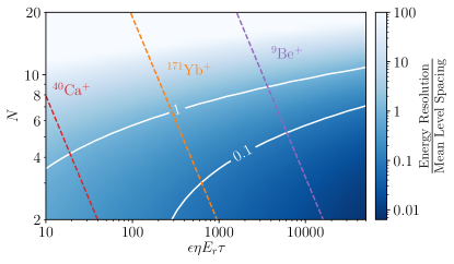
Figure 8: Energy resolution of a single run of the QND measurement for different ions species. The (dimensionless) energy resolution $\Delta E/J$ over the mean level spacing $N/2^{N}$ is plotted against the ion number $N$ and the dimensionless parameter $\epsilon\eta E_{r}\tau$, where $\epsilon$ is the detection efficency, $\eta$ the Lamb-Dicke paramter $E_{r}$ the recoil energy and $\tau$ the measurement time. The three dashed lines corresponds to estimations for three different ion species, for which we fix $\epsilon=0.15,\eta=0.1$ and choose $\tau=t_{\rm coh}/N$ with $t_{\rm coh}$ the single-spin coherence time.

We now discuss and compare the implementation with different ion species. As already mentioned in Supplementary Note XI.4.1, different ion species have different coupling strengths to the laser fields, and thus different energy scales of the targeted spin models and the associated QND measurements. Further, different ion species possess different coherence time. These parameters impact the performance of an implementation of our QND measurement scheme. As examples, we consider three ion species that are commonly used in current trapped-ion experiments: ${}^{171}{\rm Yb}^{+}$, ${}^{40}{\rm Ca}^{+}$ and ${}^{9}{\rm Be}^{+}$.

A key parameter to quantify the performance of the proposed QND measurement is the signal-to-noise ratio (SNR) of a single measurement run, see the discussion in Methods of the main text. This can be equivalently expressed in terms of the (dimensionless) energy resolution $\Delta E/J\sim 1/\sqrt{2\gamma\epsilon\tau}$, for given measurement strength $\gamma$, photon collection efficiency $\epsilon$ and filtering time $\tau$ (which is the same as the measurement time). The energy resolution represents our ability to distinguish two adjacent energy levels from the documented data of a single measurement run, and should be compared to the (dimensionless) mean many-body level spacing, which can be estimated as $N/2^{N}$.

The achievable measurement time $\tau$ can be estimated using the typical many-body dephasing time as $\tau=t_{\rm coh}/N$, with $t_{\rm coh}$ the single-spin coherence time and $N$ the number of ions. The measurement strength $\gamma$ of our QND scheme is controlled by the parameter $\vartheta J\sim(\eta/\sqrt{N})E_{r}(\Omega/\Delta)^{2}$, see the discussion in Supplementary Note XI.1. Here, $E_{r}$ is the recoil energy of the qubit transition, whereas $\Omega/\Delta\ll 1$ is a small quantity independent of the ion species. As a result, we have the energy resolution $\Delta E/J\sim(\Delta/\Omega)N^{3/4}/\sqrt{2\eta\epsilon E_{r}t_{\rm coh}}$. Taking realistic experimental parameters, we find that the quantity $\eta\epsilon E_{r}t_{\rm coh}$ differs for different ion species and spans a range from $10^{2}$ for ${}^{40}{\rm Ca}^{+}$ to $10^{4}$ for ${}^{9}{\rm Be}^{+}$, see the vertical lines in Supplementary Fig. 8. Among the three ion species, ${}^{9}{\rm Be}^{+}$ holds the promise of achieving the best energy resolution due to its light mass and long coherence time.

In Supplementary Fig. 8, we further plot the ratio between the energy resolution $\Delta E/J$ and the mean level spacing $N/2^{N}$, for increasing ion number $N$. Under current experimental conditions, the maximum system size $N$ for which a single run of the QND measurement is able to resolve the eigenenergies can be estimated as $N\simeq 4$ for ${}^{40}{\rm Ca}^{+}$, $N\simeq 6$ for ${}^{171}{\rm Yb}^{+}$ and $N\simeq 8$ for ${}^{9}{\rm Be}^{+}$. As a result, all three ion species are good candidates for building an intermediate-size interacting spin system for testing quantum fluctuation relations. The favorable scalability of ${}^{9}{\rm Be}^{+}$ facilitates testing the eigenstate thermalization hypothesis. Finally, we note that these estimations concern a single measurement run and better energy resolution could be achieved by repeated measurements.

XI.4.5 Parameters for proof-of-principle experiments

We proceed to present experimental parameters for a proof-of-principle implementation of our QND measurement scheme.

First, let us consider an implementation with ⁹Be⁺ ions and with axial phonon modes. The experimental system we have in mind is similar to the one reported in Ref. PhysRevLett.117.060505 . To be concrete, we consider $N=5$ ⁹Be⁺ ions in a linear Paul trap. The internal spin of a ⁹Be⁺ ion consists of two hyperfine states driven by a Raman transition involving two $313\,\mathrm{nm}$ single-photon transitions with recoil energy $E_{r}=2\pi\times 226.5\,\mathrm{kHZ}$. We choose the axial trapping frequency $\omega_{z}=2\pi\times 3\,\mathrm{MHz}$, leading to a moderate Lamb-Dicke parameter of $\eta\simeq\sqrt{E_{r}/\omega_{z}}\simeq 0.27$. We further choose $\Delta=3\omega_{q=4}$ and $\Omega=0.15\Delta$ to stay in the off-resonant regime. The resulting spin-spin coupling strength is $J\simeq 2\pi\times 5\,\mathrm{kHz}$, and the system-meter coupling is $\vartheta\simeq-0.17$. We choose the laser cooling rate of the ancilla ion $\gamma_{s}=2\pi\times 5\,\mathrm{kHz}$. Consequently, the effective measurement rate is $\gamma\simeq 2\pi\times 290\,\mathrm{Hz}$. Assuming a photon collection efficiency $\epsilon=0.15$ as discussed above, our QND measurement has a resulting characteristic time scale $1/\epsilon\gamma\simeq 3.7\,\mathrm{ms}$, which is much shorter than the typical single qubit dephasing time $\sim 1\,\mathrm{s}$ PhysRevLett.117.060505 . Specifically, an averaging time $\tau=10/\epsilon\gamma$ leads to an energy resolution (see Methods) $\Delta E/J\sim 0.22$, smaller than the minimal energy gap in this five-spin Ising model. This enables the preparation of single energy eigenstates via QND measurement, which suffices, e.g., for testing quantum fluctuation relations. This also allows for the observation of quantum jumps between different eigenstates in the imperfect QND regime as discussed in the main text.

Next, we provide experimental parameters for a transverse-phonon implementation realizing the power-law decaying spin-spin interactions, and discuss the associated energy resolution. These are relevant to the discussion in Supplementary Note XIII below on testing the eigenstate thermalization hypothesis. We consider $N=6$ ⁹Be⁺ ions in a linear Paul trap with axial trapping frequency $\omega_{z}=2\pi\times 2\,\mathrm{MHz}$ and transverse trapping frequency $\omega_{x}=2\pi\times 8\,\mathrm{MHz}$. We choose $\Omega=2\pi\times 1.76\,\mathrm{MHz}$, $\Delta=2\pi\times 8.8\,\mathrm{MHz}$, $\Delta^{\prime}=\Delta+\omega_{x}$, and the Lamb-Dicke parameter along the transverse direction $\eta=0.09<\sqrt{E_{r}/\omega_{x}}$, which can be realized by properly choosing the direction of the double MS beams with respect to the ion string. The resulting spin-spin coupling strength obeys an approximate power law decay $J_{ij}\sim J/|i-j|^{\alpha}$ with $\alpha=1.5$ and $J\simeq 2\pi\times 2.6\,\mathrm{kHz}$. Further, this generate a QND coupling with strength $|\vartheta J|\simeq 2\pi\times 0.1\,\mathrm{kHz}$. We choose the laser cooling rate of the ancilla ion $\gamma_{s}=2\pi\times 0.5\,\mathrm{kHz}$. Consequently, the effective measurement rate is $\gamma\simeq 2\pi\times 40\,\mathrm{Hz}$. Assuming a photon collection efficiency $\epsilon=0.15$, and a measurement time $\tau=50\,\mathrm{ms}$, the achieved energy resolution is $\Delta E/J\simeq 0.35$. This corresponds to a resolution of the energy density $\Delta\varepsilon=\Delta E/(JN)=0.06$, which is indicated as horizontal error bars in Supplementary Fig. 12.

XII Numerical study of thermal properties of energy eigenstates

In this section we provide additional details on the numerical simulations used in our study of thermal properties of the energy eigenstates in the main text.

In Supplementary Note XII.1 we describe the canonical-ensemble quantum Monte-Carlo simulations of the transverse-field Ising model used in Fig. 3 of the main text. We discuss the phase transition in the case of of long- and short-range interactions.

In Supplementary Note XII.2 we discuss the phase diagram of the transverse field Ising model for realistic spin-spin interaction $J_{ij}$ and show that it qualitatively agree with the one obtained using an approximate power-law.

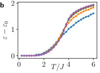
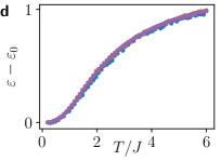
Figure 9: Phase transition of the Ising model in the canonical ensemble. (a), (c) Binder cumulant as a function of temperature for different system sizes. (b), (d) the corresponding energy of the system.

XII.1 Monte-Carlo simulations

Here we provide details on the numerical simulations of the phase transition of the Ising model in canonical ensemble $\hat{\rho}_{\text{th}}\left(T\right)\equiv e^{-\hat{H}/T}/\text{Tr}\left[e^{-\hat{H}/T}\right]$ using the quantum Monte-Carlo technique. It allows us to calculate the critical energy $\varepsilon$ using the finite-size scaling analysis of the Binder cumulant, defined as

$$U_{4}\equiv 1-\frac{\left\langle\hat{m}_{x}^{4}\right\rangle}{3\left\langle\hat{m}_{x}^{2}\right\rangle^{2}}$$

By its construction Binder81 , this cumulant distinguishes the ordered phase with $U_{4}\approx 2/3$, from the disordered phase with $U_{4}\approx 0$. As a result, when crossing the phase transition, the Binder cumulant has a sharp jump between these two values at the critical temperature $T_{c}$. This allows us to determine $T_{c}$ for the Ising model. The results of the Monte-Carlo simulation for $\alpha=1.5,$ $h/J=1$ and different system sizes $N$ are shown in Supplementary Fig. 9(a). For a sufficiently large number of spins the curves of $U_{4}$ cross approximately at the same temperature, which provides a good estimate of $T_{c}$. The corresponding critical energy density $\varepsilon\equiv\text{Tr}\left[\hat{H}\hat{\rho}_{\text{th}}\left(T_{c}\right)\right]/NJ$ can be easily determined from the energy-temperature conversion curve shown in Supplementary Fig. 9(b).

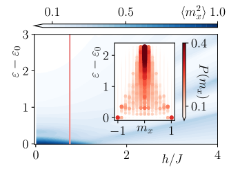
Figure 10: Excited-state phase transition in the Ising model with $\alpha=3$. (a) Ferro-paramagnet crossover in the Ising model of $N=14$ spins prepared by the energy measurements in microcanonical ensembles of width $\Delta E/(JN)=0.1$. The transition between magnetically ordered phase $\braket{\hat{m}_{x}^{2}}_{\text{mc}}\approx 1$ (dark blue) to disordered phase $\braket{\hat{m}_{x}^{2}}_{\text{mc}}\approx 0$ (light blue) is shown as function of the mean energy density $\varepsilon=\braket{\hat{H}}_{{\rm mc}}/(JN)$ and the transverse field $h$. Test of ETH for the symmetry sector $\{+1,+1\}$ is shown in the inset: only the ground state has a bimodal distribution $P\left(m_{x}\right)$.

We also study the Ising model with $\alpha=3$ shown in Supplementary Fig. 9(c) and (d). The Binder cumulant curves show no crossing at finite temperature, which indicates the absence of thermal phase transitions as it should be in case of short-range interactions $\alpha>2$ Dutta_01 . Below, we study if the same thermodynamic properties are exhibited by the individual eigenstates as can be expected if the ETH holds in this regime.

XII.2 Realistic spin-spin interaction

For a finite ion chain, the spin-spin coupling $J_{ij}$ Eq. (31) only approximately satisfy the power law. Here we study the phase diagram of the Ising model using these realistic spin-spin interaction coefficients $J_{ij}$, and show that it agrees well with the phase diagram of the power-law interaction model studied in the main text. We consider $14$ ions in a linear Paul trap and use the transverse phonons to implement our QND measurement. We choose $\omega_{x}/\omega_{z}=10$, $\Delta/\omega_{z}=10.22$ and $\Delta^{\prime}/\omega_{z}=20.22$. By numerically calculate the phonon modes, we find that the spin-spin couplings in Eq. (8) of the main text satisfy approximately power-law decay, with the exponent $\alpha\simeq 1.5$ from a least-square fit. Based on these realistic spin-spin couplings, we calculate the phase diagram of the system as is shown in Supplementary Fig. 11. As can be seen all the features of the phase diagram are in good agreement with those shown in the main text, where we approximated $J_{ij}\propto 1/|i-j|^{1.5}$.

XII.3 Case of short-range interactions

We now study the phase transition for the case $\alpha=3$ in the microcanonical ensemble and on the level of individual eigenstates. The phase diagram in the microcanonical ensemble is shown in Supplementary Fig. 10. It is clearly visible that contrary to the long-range Ising model, the ordering remains only in the vicinity of $\epsilon\approx\epsilon_{0}$. This is also reflected by the order parameter probability distribution $P\left(m_{x}\right)$ for the individual eigenstates shown in inset of Supplementary Fig. 10, which shows bimodal behavior only for the ground state. We note that this observation is compatible with the eigenstate thermalization hypothesis.

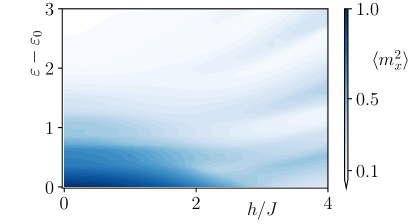
Figure 11: Phase diagram of the transverse field Ising model $N=14$ with the interaction coefficients $J_{ij}$ computed according to Eq. (31). All the qualitative features are in good agreement with those shown in Fig. 3 (a) of the main text.

XIII Eigenstate thermalization hypothesis

As explained in the main text, the ETH asserts a specific form of matrix elements of few-body observables in the energy eigenbasis of an ergodic many-body Hamiltonian Srednicki1999 :

$$\braket{\ell^{\prime}}{\hat{O}}{\ell}=O(\bar{E})\delta_{\ell^{\prime}\ell}+e^{-S(\bar{E})/2}f_{\hat{O}}(\bar{E},\omega)R_{\ell^{\prime}\ell}.$$ (55)

In particular, diagonal and off-diagonal matrix elements are determined by functions $O(\bar{E})$ and $f_{\hat{O}}(\bar{E},\omega)$, respectively, which depend smoothly on their arguments $\bar{E}=(E_{\ell}+E_{\ell^{\prime}})/2$ and $\omega=E_{\ell^{\prime}}-E_{\ell}$. $S(\bar{E})$ is the thermodynamic entropy at the mean energy $\bar{E}$, and $R_{\ell^{\prime}\ell}$ is a random number with zero mean and unit variance. From the above form of matrix elements it follows that single energy eigenstates $\ket{\ell}$ encode thermodynamic properties such as phases and phase transitions which we typically associate with a microcanonical or canonical ensemble describing systems in thermodynamic equilibrium. In the main text, we describe how qualitative aspects of eigenstate thermalization can be probed across the ferromagnetic phase transition of the long-range transverse Ising model at finite energy density. Here, we elaborate on direct and more quantitative experimental tests for diagonal and off-diagonal matrix elements.

XIII.1 Diagonal matrix elements

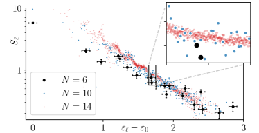
Figure 12: Structure factor for single energy eigenstates for $N=6,10,14$ (black, blue, red dots). The narrowing of fluctuations of the eigenstate expectation values with increasing system size is a clear indication of the occurrence of eigenstate thermalization. The Ising model parameters are $\alpha=1.5$ and $h/J=0.75$. The horizontal error bars indicate the estimated energy resolution for 6 spins. The vertical error bars provide an estimate of the result dispersion for 100 simulated experimental runs per eigenvalue.

Assessing ETH quantitatively requires to show that fluctuations of single-eigenstate expectation values $\braket{\ell}{\hat{O}}{\ell}$ around the microcanonical average $\mathop{\mathrm{tr}}(\hat{O}\hat{\rho}_{E_{\ell}}^{\mathrm{mc}})$ are suppressed with increasing system size DAlessio2016 . Suitable expectation values for this purpose are fluctuations of the magnetization, $\langle\ell|\hat{m}_{x}^{2}|\ell\rangle$ where $\hat{m}_{x}=N^{-1}\sum_{j}\hat{\sigma}_{j}^{x}$, and the structure factor, $S_{\ell}\equiv N\langle\ell|\hat{m}_{x}^{2}|\ell\rangle$, which remain finite in the thermodynamic limit in the ordered and disordered phase, respectively. Using these quantities, numerical tests of ETH have been performed for the two-dimensional transverse Ising model with nearest-neighbor interactions Mondaini2016 , and in the one-dimensional model Fratus2016 . In experiments with the trapped ion toolbox, the system sizes for which single eigenstates can be prepared are limited by the increasing measurement time which is required to resolve many-body energy level splittings. Since for intermediate system sizes the number of states in the disordered phase exceeds the one in the ordered phase (see Fig. 3 in the main text), the most promising prospect to test ETH quantitatively in experiments is to consider the structure factor $S_{\ell}$ in the disordered phase. We demonstrate the narrowing with system size of state-to-state fluctuations of the structure factor for the one-dimensional transverse Ising model numerically in Supplementary Fig. 12. Even for $6$ spins, for which we expect experiments with current technology to be able to resolve individual energy eigenstates as discussed in Supplementary Note XI.4.5 above, the structure factor exhibits relatively small state-to-state fluctuations, consistent with ETH. In the figure, we also indicate the estimated energy resolution for $6$ spins, and the expected error in determining the structure factor from 1000 measurements. A further suppression of state-to-state fluctuations is clearly visible for 10 and 14 spin systems, which, however, require improved experimental coherence times and detection efficiencies.

XIII.2 Off-diagonal matrix elements

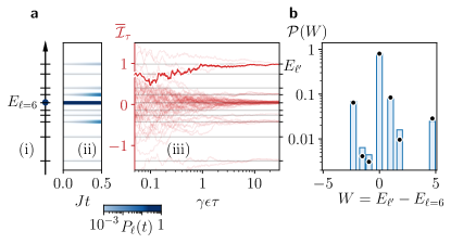
Figure 13: Measuring off-diagonal matrix elements of a local observable $\hat{V}=\tilde{h}\,\hat{\sigma}_{j}^{z}$ in the energy eigenbasis via the work probability distribution $P(W)$. (a) Protocol to measure the work distribution $P(W)$ as described in the text. (i) The system of $N=5$ spins is prepared in an energy eigenstate $\ket{\ell=6}$ with energy $E_{\ell=6}$. (ii) By applying the perturbation $\hat{V}$ at the middle spin ($j=3$ and $\tilde{h}=J$) during a time $J\Delta t=0.5$, the system is driven into a superposition of eigenstates $\ket{\ell}$ with probabilities $P_{\ell}(t)$ (blue shading). (iii) A second measurement of energy collapses the state of the system continuously to a final state $\ket{\ell^{\prime}}$. An exemplary trajectory is shown in dark red. Repeating steps (i), (ii), and (iii) produces a sample of trajectories (light red), which gives access to the full distribution $P(W)$ of work $W=E_{\ell^{\prime}}-E_{\ell}$. (b) Normalized work distribution $\mathcal{P}(W)=P(W)/\sum_{W}P(W)$ (blue columns). For weak perturbations, the work distribution is determined by off-diagonal matrix elements $\braket{\ell^{\prime}}{\hat{V}}{\ell}$ of the perturbation. The corresponding approximation to $\mathcal{P}(W)$ is indicated by black dots.

Off-diagonal matrix elements are encoded in the dynamics, e.g. in transition probabilities between energy eigenstates in response to a weak perturbation. Using the trapped-ion QND toolbox, these transition probabilities are accessible through the protocol, which is illustrated in Supplementary Fig. 13(a): The preparation (i) of an eigenstate of $\hat{H}$ with energy $E_{\ell}$ at a given value $h$ of the transverse field is followed by a period (ii) of length $\Delta t$ of free evolution [$\vartheta=0$ in Eq. (12)] according to a perturbed Hamiltonian $\hat{H}^{\prime}=\hat{H}+\hat{V}$; this is followed by another measurement (iii) of $\hat{H}$ which yields a value $E_{\ell^{\prime}}$. The measurement outcomes determine the work $W=E_{\ell^{\prime}}-E_{\ell}$ performed on the system by the perturbation $\hat{V}$. To the lowest order in the perturbation, the work distribution is determined by off-diagonal matrix elements $\braket{\ell^{\prime}}{\hat{V}}{\ell}$ in the energy eigenbasis, $P(W)=\delta_{\ell^{\prime}\ell}+\left(\Delta t\right)^{2}\lvert\braket{\ell^{\prime}}{\hat{V}}{\ell}\rvert^{2}$. For $\lvert\braket{\ell^{\prime}}{\hat{V}}{\ell}\rvert,W\ll(\Delta t)^{-1}$, we find good agreement between the exact work distribution and the lowest-order approximation as illustrated in Supplementary Fig. 13(b).

References

- (1) Parsons, M. F. et al. Site-resolved measurement of the spin-correlation function in the fermi-hubbard model. Science 353, 1253–1256 (2016).
- (2) Boll, M. et al. Spin- and density-resolved microscopy of antiferromagnetic correlations in fermi-hubbard chains. Science 353, 1257–1260 (2016).
- (3) Brydges, T. et al. Probing rényi entanglement entropy via randomized measurements. Science 364, 260–263 (2019).
- (4) Gärttner, M. et al. Measuring out-of-time-order correlations and multiple quantum spectra in a trapped-ion quantum magnet. Nat. Phys. 13, 781–786 (2017).
- (5) Negnevitsky, V. et al. Repeated multi-qubit readout and feedback with a mixed-species trapped-ion register. Nature 563, 527–531 (2018).
- (6) Roßnagel, J. et al. A single-atom heat engine. Science 352, 325–329 (2016).
- (7) Landsman, K. A. et al. Verified quantum information scrambling. Nature 567, 61–65 (2019).
- (8) Norcia, M. A., Young, A. W. & Kaufman, A. M. Microscopic Control and Detection of Ultracold Strontium in Optical-Tweezer Arrays. Phys. Rev. X 8, 041054 (2018).
- (9) Cooper, A. et al. Alkaline-Earth Atoms in Optical Tweezers. Phys. Rev. X 8, 041055 (2018).
- (10) Keesling, A. et al. Quantum kibble–zurek mechanism and critical dynamics on a programmable rydberg simulator. Nature 568, 207–211 (2019).
- (11) Barredo, D., Lienhard, V., de Léséleuc, S., Lahaye, T. & Browaeys, A. Synthetic three-dimensional atomic structures assembled atom by atom. Nature 561, 79–82 (2018).
- (12) Saskin, S., Wilson, J. T., Grinkemeyer, B. & Thompson, J. D. Narrow-line cooling and imaging of ytterbium atoms in an optical tweezer array. Phys. Rev. Lett. 122, 143002 (2019).
- (13) Barends, R. et al. Digitized adiabatic quantum computing with a superconducting circuit. Nature 534, 222–226 (2016).
- (14) Besse, J.-C. et al. Single-shot quantum nondemolition detection of individual itinerant microwave photons. Phys. Rev. X 8, 021003 (2018).
- (15) Gleyzes, S. et al. Quantum jumps of light recording the birth and death of a photon in a cavity. Nature 446, 297–300 (2007).
- (16) Johnson, B. R. et al. Quantum non-demolition detection of single microwave photons in a circuit. Nat. Phys. 6, 663–667 (2010).
- (17) Volz, J., Gehr, R., Dubois, G., Estève, J. & Reichel, J. Measurement of the internal state of a single atom without energy exchange. Nature 475, 210 (2011).
- (18) Hacohen-Gourgy, S. et al. Quantum dynamics of simultaneously measured non-commuting observables. Nature 538, 491 (2016).
- (19) Hume, D. B., Rosenband, T. & Wineland, D. J. High-fidelity adaptive qubit detection through repetitive quantum nondemolition measurements. Phys. Rev. Lett. 99, 120502 (2007).
- (20) Eckert, K. et al. Quantum non-demolition detection of strongly correlated systems. Nature Physics 4, 50 (2007).
- (21) Senko, C. et al. Coherent imaging spectroscopy of a quantum many-body spin system. Science 345, 430–433 (2014).
- (22) Deutsch, J. Quantum statistical mechanics in a closed system. Phys. Rev. A 43, 2046–2049 (1991).
- (23) Srednicki, M. Chaos and quantum thermalization. Phys. Rev. E 50, 888–901 (1994).
- (24) Rigol, M., Dunjko, V. & Olshanii, M. Thermalization and its mechanism for generic isolated quantum systems. Nature 452, 854 (2008).
- (25) Campisi, M., Hänggi, P. & Talkner, P. Colloquium: Quantum fluctuation relations: Foundations and applications. Rev. Mod. Phys. 83, 771–791 (2011).
- (26) Huber, G., Schmidt-Kaler, F., Deffner, S. & Lutz, E. Employing trapped cold ions to verify the quantum jarzynski equality. Phys. Rev. Lett. 101, 070403 (2008).
- (27) An, S. et al. Experimental test of the quantum jarzynski equality with a trapped-ion system. Nature Physics 11, 193 (2014).
- (28) Cerisola, F. et al. Using a quantum work meter to test non-equilibrium fluctuation theorems. Nature Communications 8, 1241 (2017).
- (29) McArdle, S., Endo, S., Aspuru-Guzik, A., Benjamin, S. & Yuan, X. Quantum computational chemistry. Preprint at http://arxiv.org/abs/1808.10402 (2018).
- (30) Zhang, J. et al. Observation of a many-body dynamical phase transition with a 53-qubit quantum simulator. Nature 551, 601–604 (2017).
- (31) Britton, J. W. et al. Engineered two-dimensional Ising interactions in a trapped-ion quantum simulator with hundreds of spins. Nature 484, 489–92 (2012).
- (32) Jurcevic, P. et al. Quasiparticle engineering and entanglement propagation in a quantum many-body system. Nature 511, 202 (2014).
- (33) Porras, D. & Cirac, J. I. Effective Quantum Spin Systems with Trapped Ions. Phys. Rev. Lett. 92, 207901 (2004).
- (34) Wade, A. C. J., Sherson, J. F. & Mølmer, K. Squeezing and entanglement of density oscillations in a bose-einstein condensate. Phys. Rev. Lett. 115, 060401 (2015).
- (35) Mazzucchi, G., Caballero-Benitez, S. F., Ivanov, D. A. & Mekhov, I. B. Quantum optical feedback control for creating strong correlations in many-body systems. Optica 3, 1213–1219 (2016).
- (36) Ashida, Y. & Ueda, M. Multiparticle quantum dynamics under real-time observation. Phys. Rev. A 95, 022124 (2017).
- (37) Lee, M. D. & Ruostekoski, J. Classical stochastic measurement trajectories: Bosonic atomic gases in an optical cavity and quantum measurement backaction. Phys. Rev. A 90, 023628 (2014).
- (38) Gardiner, C. & Zoller, P. The Quantum World of Ultra-Cold Atoms and Light Book II: The Physics of Quantum-Optical Devices. Cold Atoms (Imperial College Press, 2015).
- (39) Wiseman, H. M. & Milburn, G. J. Quantum Measurement and Control (Cambridge University Press, Cambridge, 2009).
- (40) Sørensen, A. & Mølmer, K. Quantum Computation with Ions in Thermal Motion. Phys. Rev. Lett. 82, 1971–1974 (1999).
- (41) Mølmer, K. & Sørensen, A. Multiparticle Entanglement of Hot Trapped Ions. Phys. Rev. Lett. 82, 1835–1838 (1999).
- (42) D’Alessio, L., Kafri, Y., Polkovnikov, A. & Rigol, M. From quantum chaos and eigenstate thermalization to statistical mechanics and thermodynamics. Adv. Phys. 65, 239–362 (2016).
- (43) Deutsch, J. M. Eigenstate thermalization hypothesis. Rep. Prog. Phys. 81, 082001 (2018).
- (44) Srednicki, M. The approach to thermal equilibrium in quantized chaotic systems. J. Phys. A. Math. Gen. 32, 1163–1175 (1999).
- (45) Fratus, K. R. & Srednicki, M. Eigenstate Thermalization and Spontaneous Symmetry Breaking in the One-Dimensional Transverse-Field Ising Model with Power-Law Interactions. Preprint at http://arxiv.org/abs/1611.03992 (2016).
- (46) Batalhão, T. B. et al. Experimental Reconstruction of Work Distribution and Study of Fluctuation Relations in a Closed Quantum System. Phys. Rev. Lett. 113, 140601 (2014).
- (47) Zhang, J. et al. Experimental test of the quantum Jarzynski equality with a trapped-ion system. Nat. Phys. 11, 193–199 (2014).
- (48) Ritsch, H., Domokos, P., Brennecke, F. & Esslinger, T. Cold atoms in cavity-generated dynamical optical potentials. Rev. Mod. Phys. 85, 553–601 (2013).
- (49) Houck, A. A., Türeci, H. E. & Koch, J. On-chip quantum simulation with superconducting circuits. Nature Physics 8, 292 (2012).
- (50) Hammerer, K., Sørensen, A. S. & Polzik, E. S. Quantum interface between light and atomic ensembles. Reviews of Modern Physics 82, 1041 (2010).
- (51) Blanes, S., Casas, F., Oteo, J. & Ros, J. The magnus expansion and some of its applications. Physics Reports 470, 151 – 238 (2009).
- (52) Linke, N. M. et al. Experimental comparison of two quantum computing architectures. Proceedings of the National Academy of Sciences 114, 3305–3310 (2017).
- (53) Johansson, J., Nation, P. & Nori, F. Qutip 2: A python framework for the dynamics of open quantum systems. Computer Physics Communications 184, 1234 – 1240 (2013).
- (54) Weinberg, P. & Bukov, M. QuSpin: a Python Package for Dynamics and Exact Diagonalisation of Quantum Many Body Systems part I: spin chains. SciPost Phys. 2, 003 (2017).
- (55) Bauer, B. et al. The ALPS project release 2.0: open source software for strongly correlated systems. Journal of Statistical Mechanics: Theory and Experiment 2011, P05001 (2011).
- (56) Kim, K. et al. Entanglement and tunable spin-spin couplings between trapped ions using multiple transverse modes. Phys. Rev. Lett. 103, 120502 (2009).
- (57) Schulz, S. A., Poschinger, U., Ziesel, F. & Schmidt-Kaler, F. Sideband cooling and coherent dynamics in a microchip multi-segmented ion trap. New Journal of Physics 10, 045007 (2008).
- (58) Harlander, M., Lechner, R., Brownnutt, M., Blatt, R. & Hänsel, W. Trapped-ion antennae for the transmission of quantum information. Nature 471, 200–203 (2011).
- (59) Mehta, K. K. et al. Ion traps fabricated in a cmos foundry. Applied Physics Letters 105 (2014).
- (60) Wilson, A. C. et al. Tunable spin–spin interactions and entanglement of ions in separate potential wells. Nature 512, 57–60 (2014).
- (61) Gardiner, C. & Zoller, P. The Quantum World of Ultra-Cold Atoms and Light Book II (ICP, London, 2015).
- (62) Cirac, J. I., Blatt, R., Zoller, P. & Phillips, W. D. Laser cooling of trapped ions in a standing wave. Phys. Rev. A 46, 2668–2681 (1992).
- (63) Wiseman, H. M. & Milburn, G. J. Quantum measurement and control (CUP, Cambridge, 2009).
- (64) Bushev, P. et al. Feedback cooling of a single trapped ion. Phys. Rev. Lett. 96, 043003 (2006).
- (65) Stute, A. et al. Toward an ion–photon quantum interface in an optical cavity. Applied Physics B 107, 1145–1157 (2012).
- (66) Tan, T. R. et al. Multi-element logic gates for trapped-ion qubits. Nature 528, 380 (2015).
- (67) Schneider, C., Enderlein, M., Huber, T. & Schaetz, T. Optical trapping of an ion. Nature Photonics 4, 772 (2010).
- (68) Langer, C. et al. Long-lived qubit memory using atomic ions. Phys. Rev. Lett. 95, 060502 (2005).
- (69) Olmschenk, S. et al. Manipulation and detection of a trapped hyperfine qubit. Phys. Rev. A 76, 052314 (2007).
- (70) Monz, T. et al. 14-qubit entanglement: Creation and coherence. Phys. Rev. Lett. 106, 130506 (2011).
- (71) Roos, C. et al. Quantum state engineering on an optical transition and decoherence in a paul trap. Phys. Rev. Lett. 83, 4713–4716 (1999).
- (72) Brown, K. R. et al. Coupled quantized mechanical oscillators. Nature 471, 196–199 (2011).
- (73) McConnell, R., Bruzewicz, C., Chiaverini, J. & Sage, J. Reduction of trapped-ion anomalous heating by in situ surface plasma cleaning. Phys. Rev. A 92, 1–5 (2015).
- (74) Wineland, D. et al. Experimental issues in coherent quantum-state manipulation of trapped atomic ions. Journal of Research of the National Institute of Standards and Technology 103, 259 (1998).
- (75) Gaebler, J. P. et al. High-fidelity universal gate set for ion qubits. Phys. Rev. Lett. 117, 060505 (2016).
- (76) Binder, K. Critical properties from monte carlo coarse graining and renormalization. Phys. Rev. Lett. 47, 693–696 (1981).
- (77) Dutta, A. & Bhattacharjee, J. K. Phase transitions in the quantum ising and rotor models with a long-range interaction. Phys. Rev. B 64, 184106 (2001).
- (78) Mondaini, R., Fratus, K. R., Srednicki, M. & Rigol, M. Eigenstate thermalization in the two-dimensional transverse field Ising model. Phys. Rev. E 93, 032104 (2016).