Impact of Network Topology on the Stability of DC Microgrids

Abstract

We probe the stability of Watts–Strogatz DC microgrids, in which droop-controlled producers and constant power load consumers are homogeneously distributed and obey Kirchhoff’s circuit laws. The concept of survivability is employed to evaluate the system’s response to Dirac delta voltage perturbations at single nodes. A fixed point analysis of the power grid model yields that there is only one relevant attractor. Using a set of simulations with random networks we investigate correlations between survivability and three topological network measures: the share of producers in the network and the degree and the average neighbour degree of the perturbed node. Depending on the imposed voltage and current limits, the stability is optimized for low node degrees or a specific share of producers. Based on our findings, we provide an insight into the local dynamics of the perturbed system and derive explicit guidelines for the design of resilient DC power grids.

More than a century ago Nicola Tesla won a victory over Thomas Edison in the war of currents and alternating current (AC) became the global standard for power grids (McPherson, 2012). Thanks to the availability of cheap AC transformers, electric energy can be transferred over thousands of kilometers through high voltage transmission lines. However, since the invention of the transistor, more and more devices are based on semiconductor technology (Brinkman, Haggan, and Troutman, 1997) and, as imposed by fundamental physics, only work with Direct Current (DC). These comprise not only every computer or LED but also environmentally friendly energy sources such as solar cells. At the same time the development of efficient power electronics which allow converting between DC voltage levels makes it possible to consider DC power grids again. Therefore, in the face of the digital transformation and this century’s need for renewable energies, the idea of DC power grids is reviving and regaining significance for the future distribution of electric energy (Dragicevic et al., 2015), in particular in the context of microgrids (Kakigano, Miura, and Ise, 2010). We simulate the electrodynamics of such small-scale networks and probe how they react to certain perturbations. Our results identify topological motives which contribute to stability and will help to design robust DC microgrids.

I Introduction

A power grid’s essential task is to ensure a reliable and stable power supply. It must be guaranteed that local events at particular nodes in the network’s infrastructure, such as a short circuit or turning on a device, do not entail a collapse of the whole system. Instead, the network should compensate the perturbation as fast and effectively as possible so that normal operation is restored. The transgression of critical current and voltage values during the system’s response, as well as a collapse into a different undesirable state (e.g. a blackout) must be strictly avoided. This raises the question how a power grid should be designed to make it robust and capable of surviving various kinds of incidents.

Besides the properties of electronic devices and transmission lines, it is the network topology of the power grid that can strongly influence the grid’s stability. Grid operators routinely perform detailed studies of their concrete systems, but by now there also exists a considerable body of work on the interplay of dynamical stability and network structure. One approach is to analytically analyse properties of the linearized AC power grid equations subject to a variety of perturbances, e.g. Grunberg and Gayme (2016); Pagnier and Jacquod (2019); Poolla, Bolognani, and Dörfler (2017); Tyloo, Coletta, and Jacquod (2018); Tamrakar, Conrath, and Kettemann (2018); Guo, Zhao, and Low (2018); Zhang et al. (2019); Plietzsch et al. (2019); Zhang, Ma, and Timme (2019). Another very successful approach to understanding the non-linear equations, and in particular towards understanding which network motives and structures are stabilizing or destabilizing in a power grid context has proceeded through probabilistic stability notions like basin stability and survivability Menck et al. (2014); Schultz, Heitzig, and Kurths (2014a); Auer et al. (2016); Hellmann et al. (2016a); Nitzbon et al. (2017a); Auer et al. (2017); Hellmann et al. (2018); Kim, Lee, and Holme (2016); Wolff, Lind, and Maass (2018). For instance, it has been found that the stability of AC power grids is undermined by dead ends in the network structureMenck et al. (2014). Subsequent works refined this in many directions, for example by studying not just individual grids but an ensemble of realistic topologies Schultz, Heitzig, and Kurths (2014b), which allowed meaningful statistics on a variety of structures. Using this ensemble, it was possible to identify specific topological structures that trigger the existence of accessible new limit cycles Nitzbon et al. (2017a).

When it comes to understanding the impact of network topology on the full non-linear system, much of what has been investigated for AC in this probabilistic manner, is still unclear for DC power grids. Recent years have seen a number of works on control strategies and consensus algorithms for DC systemsDragicevic et al. (2016); Zhao and Dörfler (2015); Meng et al. (2017); De Persis, Weitenberg, and Dörfler (2018); Cucuzzella et al. (2018); Trip et al. (2019), or more specifically HVDC systems Andreasson et al. (2014); Zonetti, Ortega, and Schiffer (2017). Further a considerable amount of work exists for single bus DC microgrids Dragicevic et al. (2016, 2015). However, for no-communication, networked (multi-terminal) DC systems the resilience of the underlying distributed power dynamics remained fairly understudied, especially outside the linear regime Anand and Fernandes (2012). Hence, in this paper, we investigate the short time scale stability of DC power grids with non-linear loads in dependence on certain topological properties of the underlying network. The systems are inspired by the application in extremely low technology scenarios encountered in the swarm electrification in rural areas of developing nationsGroh et al. (2015).

• The modelStrenge et al. (2017) describes classical electrodynamics on a complex network of uniformly distributed consumers and producers subject to communication free minimal control. It is studied analytically to show that normal operation is the only relevant attractor, which implies that stability measures made for multistable systems (like basin stability) are not helpful here.

• To find the most stable network topology, simulations are carried out using a probabilistic scheme. Randomized Watts–Strogatz Watts and Strogatz (1998) networks are perturbed locally by instant Dirac-delta-like voltage jumps at a single randomly selected node. The system’s response is then evaluated in terms of a stability measure which focuses on transient dynamics, survivability Hellmann et al. (2016b).

• The survivability is then correlated with three important topological network measures. We identify the share of producers in the power grid and the perturbed node’s degree as primary indicators of a DC power grid’s stability.

• Finally, our findings are further enriched with physical intuition and traced back to short-range interactions between current and voltage dynamics.

Our model is stylized to be able to focus on system-wide features and aims to complement electrical engineering studies that tend to focus on more detail. The structure and the parameters of the simulated networks Strenge et al. (2017) were chosen to resemble microgrids as found at remote villages without power supply in a swarm electrification approach Groh et al. (2015). In the first place such networks are built for low-power applications such as electric lighting. Although our results are obtained using this particular case, they are meant to demonstrate general motives inherent to the physics of DC power grids.

II The Model

II.1 Definition and Parameters

Our model of a unipolar DC power grid is defined by a set of differential equations which apply Kirchhoff’s circuit laws to a network graph. Edges represent power lines while nodes constitute consumer or producer units. Power lines possess both resistance $R$ and inductance $L$ and connect adjacent nodes by carrying a current $i$. The network is represented by a directed graph to unambiguously define the current direction in each edge. Each node is equipped with a capacitance $C$ and operates at a voltage labelled $v_{P}$ for producers and $v_{C}$ for consumers, respectively. In addition, the capacitor is put in parallel with either a droop-controlled voltage generator in the case of producers (droop coefficient $K$ and targeted reference voltage $v_{ref}$) or an electrical load that dissipates energy at a constant power $P_{C}<0$ (the negative sign follows the ‘generator convention’) in the case of consumers. Consumers are modeled as constant power loads to account for the power-maintaining effect of power electronic converters (DC/DC and DC/AC) which are needed to meet the voltage requirements of a load Singh, Gautam, and Fulwani (2017). The rationale for assuming Droop control for producers is to use a simple technique which achieves the basic control goal of maintaining a reference voltage in the power grid, as it has been done previously Anand and Fernandes (2012); Strenge et al. (2017). More sophisticated designs Gavriluta et al. (2014) are a matter of active research and are beyond the scope of this paper. Further, recent work mostly concerns the study of systems with communication infrastructure De Persis, Weitenberg, and Dörfler (2018); Cucuzzella et al. (2018) which we do not want to assume here.

Following the model proposed by Strenge et al. Strenge et al. (2017), the temporal evolution of node voltages (index $n$) and edge currents (index $l$) is then defined by

$$L\frac{di_{l}}{dt}=-R\,i_{l}+\sum_{adj.\;n}v_{n}\,(-1)^{d(l,n)},\;\;$$ (1)

$$C\frac{dv_{P,n}}{dt}=K\,(v_{ref}-v_{P,n})-\sum_{inc.\;l}i_{l}\,(-1)^{d(l,n)},\;\;$$ (2)

$$C\frac{dv_{C,n}}{dt}=\frac{P_{C}}{v_{C,n}}-\sum_{inc.\;l}i_{l}\,(-1)^{d(l,n)},\;\;$$ (3)

with $adj.\,n$ being the adjacent nodes and $inc.\,l$ being the incident edges (power lines). Here, all edges, producer nodes and consumer nodes are assumed to be identical within each category. The sums collect the voltage (current) contributions from all adjacent nodes (incident edges) and add them together consistently with the correct sign, according to the direction of the connected edges. The exponent $d(l,n)$ takes the value $1$ if edge $l$ points towards node $n$ and is zero otherwise. Expressed in words, the differential equations state that, on the one hand, changes in edge currents are caused by voltage gradients and Joule heating ($R\,i$). On the other hand, the node voltages respond to the net current of incident edges as well as either to a constant power load current ($P_{C}/v_{c}$) or to a droop-controlled power generation current $i_{gen,n}=K(v_{ref,P}-v_{P,n})$. This depends on whether the node is a consumer or a producer, respectively. For a network with $N_{C}$ consumers, $N_{P}$ producers, and $N_{L}$ connecting power lines, the full system in Eqns. (1–3) comprises $N_{C}$ + $N_{P}$ node equations and $N_{L}$ edge equations. Their mutual coupling is introduced by the sums over the adjacent nodes and incident edges and is determined by the underlying network topology.

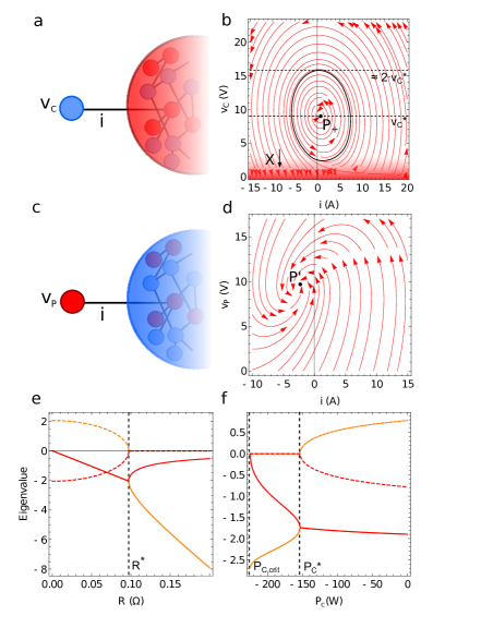
Figure 1: (a–b) The DC power grid can be approximated with a two-node graph containing only the perturbed consumer node and a ‘supernode’ representing the remainder of the network, summarized as one effective producer node with constant voltage $v_{P}$. The corresponding system of two differential equations (6) exhibits one exponentially stable fixed point $P_{+}$ (normal operation) and a voltage collapse $X$. The black curve indicates the border between the corresponding basins. (c–d) Analogously, for a producer node being perturbed, the remainder of the network acts as an effective consumer node with approximately constant voltage $v_{c}$. Then, (6) always converges to the only stable fixed point $P^{\prime}$ and normal operation is ensured. (e–f) Real (solid) and imaginary (dashed) parts of the eigenvalues (red and orange) of the Jacobi matrix at $P_{+}$, shown as a function of wire resistance $R$ and consumer power $P_{C}$. The attractor has a higher convergence speed for low $R$ and low $|P_{C}|$ and forms a stable focus if $R<R^{\ast}$ or $P_{C}>P_{C}^{\ast}$. $R^{\ast}$ and $P_{C}^{\ast}$ are the bifurcations which mark the transition from a stable node to a stable spiral (or vice versa).

II.2 Equilibrium Voltage

At normal operation, the total power fed into the system by $N_{P}$ producers and the power drawn by $N_{C}$ consumers must add up to zero. Neglecting Joule heating in the power lines we can write

$$N_{P}P_{P}+N_{C}P_{C}=0.$$ (4)

Here, $P_{P}=\sum_{n}P_{P,n}/N_{P}$ denotes the average power production per producer, with $P_{P,n}=v_{P,n}\,i_{gen,n}$ being the product of the producer’s node voltage $v_{P,n}$ and its power generating current $i_{gen,n}=K(v_{ref}-v_{P,n})$. If consumers and producers are uniformly distributed in all regions of the network, i.e.  without forming clusters, all node voltages will equilibrate close to the overall average voltage $v_{eq}$, so that $v_{P,n}\approx v_{eq}$ and $P_{P}\approx v_{eq}K(v_{ref}-v_{eq}).$ Then (4) can be solved for $v_{eq}$,

$$v_{eq}(s)=\frac{v_{ref}}{2}+\sqrt{\frac{v_{ref}^{2}}{4}-\frac{1-s}{s}\frac{P_{C}}{K}},$$ (5)

where $s=N_{P}/(N_{P}+N_{C})$ is the share of producers in the network. The solution in (5) approaches $v_{ref}$ in the limit of producer saturation ($s=1$) and collapses for $s<s_{crit}=P_{C}/(P_{C}-Kv_{ref}^{2}/4)$. In the latter case, the total energy generated at producer nodes falls short of serving the total energy demanded by consumers. Note that this attractive singularity is always present. For a sufficiently small voltage at a consumer node the $P_{C}/v_{C}$ term in (3) dominates and the system hits the singularity $v=0$ in finite time. We will return to the possibility of this voltage collapse later.

II.3 Two-Node Approximations

The term $P_{C}/v_{C,n}$ in (3) expresses the rigid attempt of a consumer node to draw energy at constant power, such that a lower node voltage $v_{C}$ is immediately compensated by drawing more current from incident edges. With $v_{C}$ in the denominator, Eqns. (1–3) represent a non-linear system and thus, in combination with a graph-based power grid structure, drive the dynamics of the complex network. While a detailed theoretical study of the full system’s dynamics is beyond the scope of this paper, grouping nodes into super-nodes with effective properties does allow to derive approximations for the overall behavior of the power grid.

When the normal operation of the network is locally perturbed by a sudden voltage jump at one single node, the interaction of the affected node with the remainder of the network can threaten the stability of the power grid. Both the exceedance of particular current or voltage values and the relaxation into a different equilibrium (e.g. collapse), rank among the undesirable scenarios which may occur during the system’s journey through the $2(N_{P}+N_{c}+N_{L})$-dimensional phase space. We assume that for sufficiently small perturbations or sufficiently large networks the average voltage in the remainder of the network will not change significantly in response to the local perturbation. From a physical point of view, the validity of this assumption arises from the node capacitors, which are put in parallel by the network structure, such that the total capacitance becomes very large. Thus, it is comparably easy for a local perturbation to change one node voltage, but very difficult to change node voltages all over the network far away from the perturbed node. Hence, we model the interaction of the perturbation with the power grid simply with a two-node network, in which the first node is the perturbed node and the second node summarizes the remainder of the network at fixed voltage. This infinite grid approximation is also typical in AC power grid studies (Kozhaya, Nassif, and Najm, 2002). Although its range of validity will require further study, it makes the model analytically tractable and gives valuable insights consistent with our simulations.

II.3.1 Perturbation at a Consumer Node

Applying this approximation to a perturbation at a consumer node (Fig. 1a), the full system of Eqns. (1–3) reduces to only two differential equations,

$$L\frac{di}{dt}=v_{P}-v_{C}-Ri,\;\;\;\;C\frac{dv_{C}}{dt}=i+\frac{P_{C}}{v_{C}}.\;\;$$ (6)

(6) yields two fixed points $P_{\pm}=(i_{\pm}^{\ast},v_{C\pm}^{\ast})$ located at

$$P_{\pm}=\left(\frac{v_{P}\mp\sqrt{4P_{C}R+v_{P}^{2}}}{-2R},\frac{v_{P}\pm\sqrt{4P_{C}R+v_{P}^{2}}}{2}\right).$$ (7)

As illustrated in Fig. 1b for $R=$0.09\text{\,}\mathrm{\SIUnitSymbolOhm}$$, $P_{C}=$-5\text{\,}\mathrm{W}$$, $C=$1\text{\,}\mathrm{F}$,L=$1\text{\,}\mathrm{H}$$ and $v_{P}=$9\text{\,}\mathrm{V}$$, the fixed point $P_{+}$ is exponentially stable. This is the desired equilibrium state of the system corresponding to normal operation. $P_{-}$, however, is located at a negative voltage and, thus, considered a non-physical solution.

In addition to these two fixed points, just like the full system, the reduced system (6) might collapse into $v_{C}=0$ which corresponds to a breakdown of the power grid ($X$ in Fig. 1b). As noted above, for $v_{C}\ll 1$, the term $P_{C}/v_{C}$ in (6) with $P_{C}<0$ dominates causing a rapid voltage decrease from which the system does not recover. The controller tries to draw more power by lowering the voltage but can not generate sufficient current to reach the desired constant power load and hits the singularity at $v_{C}=0$ in finite time. The red region in Fig. 1b indicates the regime in which the voltage collapse occurs.

The trajectory towards the attractor $P_{+}$ pictures a converging spiral (Fig. 1b), hence it is a stable focus. This behavior is consistent with the pair of complex conjugated eigenvalues of the corresponding Jacobi matrix, as seen in Fig. 1e and f for $R<R^{\ast}$ and $P_{C}>P_{C}^{\ast}$. At the bifurcations $R=R^{\ast}$ and $P_{C}=P_{C}^{\ast}$ the two eigenvalues become real and the focus of $P_{+}$ transforms into a stable node. The convergence rates of both spiral and node are given by the real part of the eigenvalues. Subsequently, the system is expected to approach $P_{+}$ faster for a lower wire resistance and less energy consumption at the consumer node. Otherwise, if the consumer power exceeds a critical value ($P_{C}<P_{C,crit}$), the square roots in (7) are complex, the fixed points $P_{\pm}$ vanish and the voltage collapse remains the only attractor the system can converge to.

Whether the power grid enters normal operation at $P_{+}$ or collapses ($X$) depends on the initial conditions $(i_{0},v_{C,0})$ imposed by the type and the strength of the perturbation. For voltage perturbations, the particular form and position of the focus in state space (Fig. 1b) allows to estimate the upper and lower limits of $v_{C}$, within which a perturbation does not lead to a collapse of the power grid: When a node is abruptly charged or discharged, the difference in energy $\Delta E_{C}=1/2\,C(v_{C,0}^{2}-{v_{C}^{\ast}}^{2})$ triggers a current $i$. However, after the injected energy has been transferred to the incident power lines ($1/2\,Li^{2}=\Delta E_{C}$), the current does not stop immediately, but, while declining, continues to further discharge the consumer node almost by another energy quantity $\Delta E_{C}$, due to the inductance of the wire. This causes the first kick in the temporal evolution of $v_{c}$ to be delimited by approximately $[v_{C}^{\ast}-|v_{c,0}-v_{C}^{\ast}|,v_{C}^{\ast}+|v_{c,0}-v_{C}^{\ast}|]$, provided that the convergence rate to the attractor is not too high. Since the basin of attraction of the focus nearly touches zero consumer voltage, the perturbation must either bring the node voltage very close to zero or exceed twice the equilibrium voltage (5) to leave the basin of $P_{+}$ and to entail the collapse X into the red region in Fig. 1b. This is why stability measures based solely on basin size (basin stability) are not a helpful tool here and one has to consider the transient behaviour to distinguish different degrees of stability against non-infinitesimal perturbations.

II.3.2 Perturbation at a Producer Node

Analogously to the case when the perturbation strikes a consumer node, the simplified system for a producer node (Fig. 1c) reads

$$L\frac{di}{dt}=v_{P}-v_{C}-Ri,\;\;$$ (8)

$$C\frac{dv_{P}}{dt}=-i+K(v_{ref}-v_{P}).\;\;$$ (9)

Eqns. (8–9) always converge to the only and exponentially stable fixed point

$$P^{\prime}=\left(\frac{K(-v_{C}+v_{ref})}{1+KR},\frac{v_{C}+KRv_{ref}}{1+KR}\right),$$ (10)

which, just like $P_{+}$, corresponds to the state of normal operation. Hence, in contrast to a perturbation at a consumer node, the power grid does not enter a different attractor if a producer node is perturbed (Fig. 1d).

In summary, the study of equilibrium states and non-equilibrium dynamics suggests that for voltage perturbations applied to individual nodes, the power grid reliably returns to normal operation without collapsing into a different attractor. The collapse regime $X$ is only relevant under extreme conditions that lie beyond the interest of our investigation. This conclusion is valid for the reduced systems of equations (6) and (8–9) which approximate the full network. In the realm of AC power grids, there is a profusion of attractors, including anomalous ones that can not be understood in the reduced way Nitzbon et al. (2017a). However, it appears that the same is not the case for the DC system since during all numerical tests involving a wide range of parameters no other stable attractors than those denoted above with $P_{+}$ or $P^{\prime}$ (normal operation) and the collapse $X$ have ever been observed in our model. Therefore, our assessment of DC power grids in terms of stability must be based on measures which evaluate the system’s trajectory inside the only relevant basin of attraction of normal operation around $P_{+}$ or $P^{\prime}$, respectively. For this purpose, we apply the probabilistic concept of survivabilityHellmann et al. (2016b), which is introduced in the following section.

III Simulation Methods

Network Parameters
Network Model	Watts–Strogatz
Rewiring Probability	$[0,1]$
Number of Nodes ($N_{C}+N_{P}$)	$[10,100]$
Mean Degree	$2,4,6$
Simulation Parameters
Producer Share ($s$)	$[0,1]$
Droop Coefficient ($K$)	$1\text{\,}\mathrm{\SIUnitSymbolOhm}^{-1}$
Power Line Inductance ($L$)	$0.237\cdot 10^{-4}$ $\mathrm{H}$
Node Capacitance ($C$)	$0.01\text{\,}\mathrm{F}$
Resistance ($R$)	$0.0532\text{\,}\mathrm{\SIUnitSymbolOhm}$
Reference Voltage ($v_{ref})$	$48\text{\,}\mathrm{V}$
Consumer Load Power ($P_{C}$)	$-12\text{\,}\mathrm{W}$
Voltage Perturbation	[$44\text{\,}\mathrm{V}$, $48\text{\,}\mathrm{V}$]
Survivability Limits
Voltage	[$44\text{\,}\mathrm{V}$, $48\text{\,}\mathrm{V}$]
Current	[$-9\text{\,}\mathrm{A}$, $9\text{\,}\mathrm{A}$]

Table 1: Physical properties of the perturbed DC power grids including voltage and current limits used for the survivability measure.

We simulated DC Power Grids on Watts–Strogatz networks by integrating Eqns. (1–3) with a step size of $20\text{\,}\mathrm{\SIUnitSymbolMicro s}$. For each simulation, the parameters of the Watts–Strogatz model (rewiring probability, number of nodes, mean degree) as well as the producer share were randomly chosen from fixed intervals (Tab.  1). Our parameter choice is an example for one particular DC microgrid. However, the same qualitative behaviour of the system was also observed for other values, including a variation of the node capacitance and the wire resistance over two orders of magnitude. The minimum number of nodes in a network was set to $10$ and the maximum number of nodes was $100$. The mean degree did not exceed six to ensure a non-trivial and, thus, more realistic, not excessively connected network topology. Other network parameters not in the focus of this study (consumer power consumption, reference voltage, power line resistance, capacity and droop coefficient) were set to constant values Strenge et al. (2017) (cf. Tab. 1).

Every simulation was initiated with zero current on all edges and with the reference voltage $v_{ref}=$48\text{\,}\mathrm{V}$$ at all nodes. To calculate the equilibrium state of normal operation, each grid was simulated for $0.2\text{\,}\mathrm{s}$ without perturbation. Subsequently, one perturbation was applied to a single node, randomly chosen from the nodes of the network. The perturbation constitutes an instant voltage jump with a new voltage value randomly selected from the interval [$44\text{\,}\mathrm{V}$, $48\text{\,}\mathrm{V}$]. From this point on, the response of the system, e.g. all voltages and currents in the network, was recorded over time until it had converged back to its previous equilibrium state. This usually took up to $0.1\text{\,}\mathrm{s}$. If currents or voltages exceed particular boundaries during the simulation, the simulation run is counted as not survived, otherwise as survived. The applied permissible voltage and current intervals read [$44\text{\,}\mathrm{V}$, $48\text{\,}\mathrm{V}$] and [$-9\text{\,}\mathrm{A}$, $9\text{\,}\mathrm{A}$], respectively, and were chosen to model a DC microgrid, which currently is the most common application of DC power grids Dragicevic et al. (2016); Backhaus et al. (2015); Dragicevic et al. (2015). Any state of the system inside the boundaries does, by far, not trigger a collapse scenario. The sequence of locally perturbing a random node and recording the response was repeated 100,000 times, creating a set of random simulations.

The share of survived simulations is called the survivability of this specific set. Survivability can be interpreted as the probability for a system to survive a random perturbation which does not kill the system instantaneously Hellmann et al. (2016b). Here, it is chosen as a primary measure, as it combines many physical effects into one quantification of stability. This allows the identification of the functionality-controlling parameters, prior to understanding all complex physical interactions of the model. Desirable network parameters are those which lead to a high survivability of a set of networks.

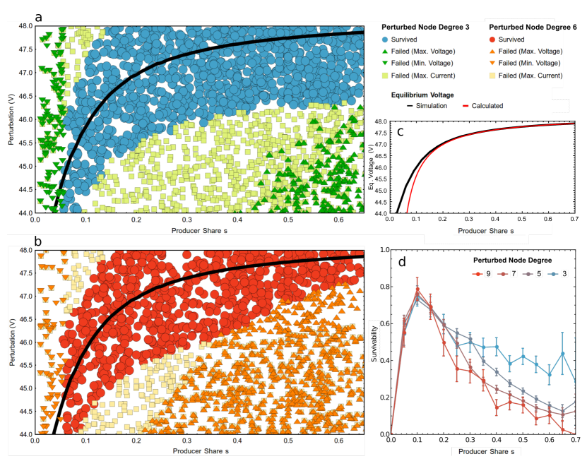
Figure 2: Randomly generated DC power grids on Watts–Strogatz graphs are locally perturbed and assessed in terms of survivability. (a) Each marker corresponds to the outcome of one simulation (survived or failed) with perturbations at nodes with degree 3. Plotted as a function of the perturbation voltage (ranging from $44\text{\,}\mathrm{V}$ to $48\text{\,}\mathrm{V}$) and the share of producers in the perturbed network, they form a band of survived simulations: It surrounds the average equilibrium voltage (black line) and is mostly delimited by violations of the current boundary ($9\text{\,}\mathrm{A}$). (b) For perturbed nodes with a higher degree of 6, the band is narrowed by violations of the upper voltage boundary $48\text{\,}\mathrm{V}$. (c) The analytically derived equilibrium voltage (5) agrees well with the simulation. (d) Since the vertical height of the band of survived simulations corresponds to the survivability as a function of producer share, the chosen voltage boundaries cause the survivability to become maximal at a producer share of $12\pm 3~{}\%$. Beyond this threshold, higher node degrees imply less stability.

IV Simulation Results

IV.1 Average Equilibrium Voltage

The average equilibrium voltage in the power grid is predicted to be related to the producer share through (5). The simulated values match the theoretical prediction almost perfectly (Fig. 2c). Merely for low-producer shares the agreement deteriorates. For $s$ approaching $s_{crit}$, fewer producers feed more consumers and, due to an increased difference between consumer and producer voltages, the approximation $v_{eq}\approx v_{P}$ in the derivation of (5) is not well fulfilled anymore.

IV.2 Band of Survived Simulations

Fig. 2a and b depict the outcomes (survived or failed) of about 4000 simulations as a function of both the share of producers in the network and the induced voltage perturbation. With one marker per simulation, the data is sorted by the degree of the perturbed node (3 in fig. 2a and 6 in fig. 2b). As suggested in Section II.3.1, the average equilibrium voltage is of substantial importance for the perturbation interval within which simulations survive. From Fig. 2a and b it is apparent that a crucial condition for survivability lies in a small perturbation magnitude relative to the average equilibrium voltage. Markers representing survived simulations form a band which is centered symmetrically around the simulated average equilibrium voltage line (black curve).

IV.3 Voltage and Current Failures

The simulations which do not survive are those whose perturbation voltage lies too far away from the average equilibrium voltage (black curve), i.e. beyond the edge of the band of survived simulations. Either the current or the voltage limits are violated during the system’s temporal evolution. As apparent from Fig. 2a and b, in the vast majority of simulations it is the current boundary of $9\text{\,}\mathrm{A}$ which causes the power grid to fail and which confines the band of survived simulations to its narrow range around the average equilibrium voltage. Failures due to current violations occur independently of the perturbed node’s degree. In the regimes of high and very low producer shares, a violation of voltage limits is observed. Minimum voltage violations below a producer share of $4\,\%$ are attributed to the observation that the average equilibrium voltage falls below the lower voltage boundary. Maximum voltage violations are suppressed for small node degrees: Perturbed nodes with a degree of 6 (Fig. 2b) are much more likely to exceed the upper voltage boundary compared to those with a lower node degree of 3 (Fig. 2a). In the former case (Fig. 2b), the sensitivity of the power grid towards voltage failures, even for perturbations very close to the equilibrium voltage, is so high that the band of survived simulations is narrowed on its bottom side at high producer shares.

IV.4 Survivability

Applying the survivability measure to Fig. 2a or b means counting the share of survived simulations (i.e.  those simulations whose voltage and current values remained within their respective bounds) along the vertical axis for all producer shares on the horizontal axis. The result of this procedure is shown in Fig. 2d which summarizes the relationship between a power grid’s survivability and the perturbed node’s degree as a function of producer share. The survivability is maximized for a particular producer share of about $12\,\%$. This maximum is a consequence of both the upper and the lower voltage boundaries which have been set to $48\text{\,}\mathrm{V}$ and $44\text{\,}\mathrm{V}$, respectively. As seen in Fig. 2a and b, these limits crop the vertical width of the band at high and low producer shares. In these regimes, the share of survived simulations within the perturbation voltage interval under consideration is diminished and results in a lower survivability. Both trends combined entail a survivability maximum at an intermediate producer share value of about $12\%$. However, if the upper voltage limit is raised (lowered), so that a different proportion of the survivability band is cut off, the region of largest vertical width of the band, and thus the region of optimal survivability, broadens (narrows) asymmetrically to the right (left), i.e.  to higher (lower) producer shares (not shown). Hence, the producer share parameter demonstrates how optimal network parameters (highest stability) depend on the boundaries of the survivability measure. This is why, in order to build the optimal DC power grid, one needs to know precisely the range of permissible voltage and current values.

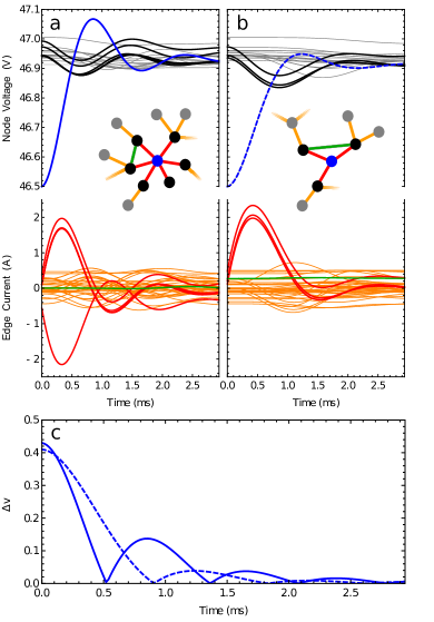
Figure 3: (a-b) More neighbours (black) cause the perturbed node (blue) to overcompensate the perturbation and to attain more extremal voltage values. This is apparent from comparing the temporal evolution of node voltages and edge currents in response to a perturbation ($46.5\text{\,}\mathrm{V}$) at a node with a high degree of 6 (a) and a low degree of 3 (b). Colors encode the proximity to the epicentre, as indicated in the schematic network graph (inset): The environment of the perturbed node (blue) is categorized into first-order edges (red), higher order edges (orange), first-order bridging edges (magenta). first-order neighbours (black) and higher-order neighbours (gray). The perturbation at $t=0$ causes the DC power grid to perform a damped wave, whose period length and damping coefficient is enhanced for the low-degree node. As the spreading of the electrical potential to adjacent neighbours is roughly isotropic, bridging edges remain unaffected by the perturbation. (c) Absolute deviation $\Delta v=|v-v_{eq}|$ of the perturbed node voltages from their equilibrium values (dashed: degree 3, normal: degree 6).

IV.5 Node Degree

In order to explain the observed differences between perturbations at nodes with a lower and higher degree, we take a closer look at the perturbed node. In Fig. 3 we juxtapose a voltage perturbation of $46.5\text{\,}\mathrm{V}$ at a consumer node with degree 3 (Fig. 3b) and at a consumer node with degree 6 (Fig. 3a). The insets picture the environments of the perturbed nodes (blue), including their incident edges (red) and adjacent nodes (black) as well as second order neighbouring edges (yellow) and nodes (grey) and first-order bridging edges (green). The plotted curves in corresponding colors depict the voltage and current evolution over time after the out-of-equilibrium voltage perturbation at $t=0$. The sudden voltage jump triggers a damped oscillation of the node voltages and edge currents. While the voltage of the perturbed node (blue) starts oscillating immediately after the perturbation, higher order neighbours and power lines are affected with a delay, depending on the distance to the epicentre. In addition, also the amplitude of the oscillation is diminished further away from the perturbed node: These nodes are only affected indirectly and the intermediate nodes screen the perturbation. First-order bridging edges (green) do not exhibit any current oscillations, as adjacent nodes are equally distant from the perturbed node and, during the radially expanding perturbation wave, experience roughly the same electrical potential.

Contrasting the responses to perturbations at nodes with different degrees, one can see a pronounced attenuation of the voltage and current oscillations at the node with degree 3 (Fig. 3b). In particular, the perturbed node with higher degree experiences a faster voltage oscillation with an amplitude declining more slowly. This is due to the initial voltage drop being overcompensated by more current from more incident power lines, which results in a subsequent voltage overshoot higher above the equilibrium voltage. Fig. 3c depicts the absolute deviation of the perturbed node’s voltage from its equilibrium value $\Delta v=|v-v_{eq}|$ and particularly highlights this observation. Hence, some power grids do not survive the perturbation because the voltage overshoot might lead to a violation of voltage boundaries. This scenario is more probable when the average equilibrium voltage lies closer to the upper voltage boundary of the survivability measure, what is the case for a large share of producers in the network (cf. Fig. 2c). Then, the survivability is diminished depending on the degree of the perturbed node (cf. Fig. 2d).

Figure 4: As the perturbation response declines fast in both time and space, the fate of the power grid is decided within the radius of first-order neighbours of the perturbed node and during the first period length of voltage and current oscillations. Thus, for a producer share $s=0.5$, one observes a distinct correlation between the survivability and the perturbed node’s degree (a), while higher-order measures, such as the perturbed node’s average neighbour degree (b), do not exhibit this feature.

The vulnerability of high degree nodes towards undesirable voltage peaks can also be understood from the eigenvalue profile depicted in Fig. 1e. The more neighbours a node has, the more edges connect the perturbed node with the remainder of the network, summarized as one supernode (cf. Fig. 1a and c). These edges are in parallel configuration, which, according to Kirchhoff’s circuit laws, lowers the total resistance of the connection. From Fig. 1e it is apparent that a lower resistance entails a lower convergence rate of the focus around the state of normal operation. As a consequence, the likelihood of striking more extremal voltage or current values in phase space is enhanced and the survivability decreases.

Therefore, apart from the magnitude of the perturbation and the producer share (global network parameter) the degree of the perturbed node (local parameter) is another potent predictor for a DC power grid’s survivability (Fig. 4a). Higher-order measures like the perturbed node’s average neighbour degree do not exhibit such a correlation (Fig. 4b). In accordance with the black, grey and orange curves in Fig. 3a and b, this is because the perturbation is damped fast not only in time but also in space, mainly within the radius of first-order neighbours.

Interestingly, our results stand in contrast with stability studies regarding AC networks. Menck et al.Menck et al. (2014) investigated the stability of AC power grids using the global average of the single-node basin stability. They found a strong influence of the perturbed node’s average neighbour degree on the power grid’s stability, whereas they found close to no influence of the first-order node degree on the power grid’s stability. However, in a different studyNitzbon et al. (2017b), it was shown with survivability that at least for specific classes of nodes, the so called sprouts, the neighbour degree has also a significant impact on the dynamics, even leading to novel bifurcations.

V Concluding Remarks

We have examined the stability of DC power grids responding to a single-node voltage perturbation. We believe such an incident to be representative for various other common power grid perturbations like a sudden load increase or a short circuit. Both trigger a voltage and current wave expanding from the epicentre into the remainder of the network.

The stability of a power grid is defined as its ability to return to normal operation after the perturbation. Trespassing certain thresholds jeopardizes this ability. For our DC microgrids, we have assumed that single-node voltages should neither fall below $44\text{\,}\mathrm{V}$ nor exceed 48V, nor should single-edge currents exceed $9\text{\,}\mathrm{A}$. If a simulated perturbed network stays within the desirable regime it is counted as survived, otherwise as not survived. Thus, applied to a single case, the survivability expresses whether a power grid (network model) of a certain configuration survives a given perturbation. Additionally, it serves as a frequentist measure of the proportion of simulated network models with certain configuration parameters surviving a given perturbation.

The producer share and the first-order node degree of the perturbed node (i.e.  the number of adjacent neighbours) are the network parameters with the highest impact on the survivability. We have found this through numerical simulations of perturbed multi-node networks in combination with analytic considerations of a two-node approximated network model. Based on these results we can provide the following guidelines for designing a DC power grid capable of surviving the investigated perturbations. If the voltage survivability limits of a DC power grid are chosen close enough to the equilibrium voltage, in other words, if large voltage deviations should be avoided, a particular producer share maximizes the survivability of the grid. In our particular case ($[$44\text{\,}\mathrm{V}$,$48\text{\,}\mathrm{V}$]$) the survivability of simulated network models is optimized for a producer share of $12\,\%$. For producer shares larger than this optimal value, the survivability is enhanced for lower node degrees. This means critical consumers or producers should be connected to as few neighbouring nodes as possible. If one keeps the real-world constraint of ”$N-1$ stability” which requires the network to stay connected if a single line breaks down, then the configuration which minimizes the number of neighbouring nodes for all nodes is a ring structure. For a DC power grid with a producer share smaller than the optimal value, the node degree does not affect its survivability, provided that the lower voltage survivability limit lies sufficiently below the band of survived simulations (cf. Fig. 2a).

We emphasize that our results contrast previous research on the stability of AC power grids. Menck et al.(Menck et al., 2014) found the average neighbour degree of the perturbed node to have a much stronger influence on the stability of the AC grid than the degree of the perturbed node itself. In contrast, for DC grids, we have not found any distinct influence of the average neighbour degree on the stability. (cf. Fig. 4). However, it is noted that a different measure of stability, survivability instead of the single-node basin stability, has been used in our investigation.

By combining voltage and current limits, the survivability represents an intuitive and overarching but also flexible measure which can be applied to both individual and multitudes of grouped network models. Yet, information regarding the individual voltage and current effects on the network is lost and has to be obtained with different methods. The single-node basin stability is not a suitable stability measure for DC power grids, because there is only one relevant attractor in the investigated parameter regime.

Further research is needed to explore stability measures for power grids in more detail. Since the survivability allows a flexible definition of boundaries, more standardized measures and limit values are required for comparative studies. More heterogeneous network models can be simulated to expand our findings to more realistic scenarios. One possibility is to investigate various control schemes suggested in the literature (Bouzid et al., 2015; Colak et al., 2015; Molzahn et al., 2017) as well as trade-offs between achieving constant power at the consumer nodes and stabilizing behaviour. Moreover, going beyond voltage kicks at single nodes, other perturbation types such as step-like sequences or white voltage (or current) noise remain to be investigated. Our stability analysis is easily extendable to a plethora of additional network measures (including centrality, transitivity and efficiency) or performance measuresPaganini and Mallada (2017). These suggestions are next steps towards finding the optimal design of stable DC power grids.

References

References

- McPherson (2012) S. S. McPherson, War of the Currents: Thomas Edison vs Nikola Tesla (Twenty-First Century Books, 2012).
- Brinkman, Haggan, and Troutman (1997) W. F. Brinkman, D. E. Haggan, and W. W. Troutman, IEEE Journal of Solid-State Circuits 32, 1858 (1997).
- Dragicevic et al. (2015) T. Dragicevic, X. Lu, J. Vasquez, and J. Guerrero, IEEE Transactions on Power Electronics , 1 (2015).
- Kakigano, Miura, and Ise (2010) H. Kakigano, Y. Miura, and T. Ise, IEEE Transactions on Power Electronics 25, 3066 (2010).
- Grunberg and Gayme (2016) T. W. Grunberg and D. F. Gayme, IEEE Transactions on Control of Network Systems 5, 456 (2016).
- Pagnier and Jacquod (2019) L. Pagnier and P. Jacquod, PLOS ONE 14, 1 (2019).
- Poolla, Bolognani, and Dörfler (2017) B. K. Poolla, S. Bolognani, and F. Dörfler, IEEE Transactions on Automatic Control 62, 6209 (2017).
- Tyloo, Coletta, and Jacquod (2018) M. Tyloo, T. Coletta, and P. Jacquod, Physical review letters 120, 084101 (2018).
- Tamrakar, Conrath, and Kettemann (2018) S. Tamrakar, M. Conrath, and S. Kettemann, Scientific reports 8, 6459 (2018).
- Guo, Zhao, and Low (2018) L. Guo, C. Zhao, and S. H. Low, in 2018 IEEE Conference on Decision and Control (CDC) (IEEE, 2018) pp. 158–165.
- Zhang et al. (2019) X. Zhang, S. Hallerberg, M. Matthiae, D. Witthaut, and M. Timme, Science Advances 5 (2019), 10.1126/sciadv.aav1027, https://advances.sciencemag.org/content/5/7/eaav1027.full.pdf .
- Plietzsch et al. (2019) A. Plietzsch, S. Auer, J. Kurths, and F. Hellmann, arXiv preprint arXiv:1903.09585 (2019).
- Zhang, Ma, and Timme (2019) X. Zhang, C. Ma, and M. Timme, arXiv preprint arXiv:1908.00957 (2019).
- Menck et al. (2014) P. J. Menck, J. Heitzig, J. Kurths, and H. Joachim Schellnhuber, Nature Communications 5, 3969 (2014).
- Schultz, Heitzig, and Kurths (2014a) P. Schultz, J. Heitzig, and J. Kurths, New Journal of Physics 16, 125001 (2014a).
- Auer et al. (2016) S. Auer, K. Kleis, P. Schultz, J. Kurths, and F. Hellmann, The European Physical Journal Special Topics 225, 609 (2016).
- Hellmann et al. (2016a) F. Hellmann, P. Schultz, C. Grabow, J. Heitzig, and J. Kurths, Scientific reports 6, 29654 (2016a).
- Nitzbon et al. (2017a) J. Nitzbon, P. Schultz, J. Heitzig, J. Kurths, and F. Hellmann, New Journal of Physics 19, 033029 (2017a).
- Auer et al. (2017) S. Auer, F. Hellmann, M. Krause, and J. Kurths, Chaos: An Interdisciplinary Journal of Nonlinear Science 27, 127003 (2017).
- Hellmann et al. (2018) F. Hellmann, P. Schultz, P. Jaros, R. Levchenko, T. Kapitaniak, J. Kurths, and Y. Maistrenko, arXiv preprint arXiv:1811.11518 (2018).
- Kim, Lee, and Holme (2016) H. Kim, S. H. Lee, and P. Holme, Physical Review E 93, 062318 (2016).
- Wolff, Lind, and Maass (2018) M. F. Wolff, P. G. Lind, and P. Maass, Chaos: An Interdisciplinary Journal of Nonlinear Science 28, 103120 (2018).
- Schultz, Heitzig, and Kurths (2014b) P. Schultz, J. Heitzig, and J. Kurths, The European Physical Journal Special Topics 223, 2593 (2014b).
- Dragicevic et al. (2016) T. Dragicevic, X. Lu, J. C. Vasquez, and J. M. Guerrero, IEEE Transactions on Power Electronics 31, 3528 (2016).
- Zhao and Dörfler (2015) J. Zhao and F. Dörfler, Automatica 61, 18 (2015).
- Meng et al. (2017) L. Meng, Q. Shafiee, G. F. Trecate, H. Karimi, D. Fulwani, X. Lu, and J. M. Guerrero, IEEE Journal of Emerging and Selected Topics in Power Electronics 5, 928 (2017).
- De Persis, Weitenberg, and Dörfler (2018) C. De Persis, E. R. Weitenberg, and F. Dörfler, Automatica 89, 364 (2018).
- Cucuzzella et al. (2018) M. Cucuzzella, S. Trip, C. De Persis, X. Cheng, A. Ferrara, and A. van der Schaft, IEEE Transactions on Control Systems Technology 27, 1583 (2018).
- Trip et al. (2019) S. Trip, M. Cucuzzella, X. Cheng, and J. Scherpen, IEEE Control Systems Letters 3, 174 (2019).
- Andreasson et al. (2014) M. Andreasson, M. Nazari, D. V. Dimarogonas, H. Sandberg, K. H. Johansson, and M. Ghandhari, IFAC Proceedings Volumes 47, 11910 (2014).
- Zonetti, Ortega, and Schiffer (2017) D. Zonetti, R. Ortega, and J. Schiffer, IEEE Transactions on Control of Network Systems 5, 1110 (2017).
- Anand and Fernandes (2012) S. Anand and B. Fernandes, IEEE Transactions on Industrial Electronics 60, 5040 (2012).
- Groh et al. (2015) S. Groh, D. Philipp, B. E. Lasch, and H. Kirchhoff, in Decentralized Solutions for Developing Economies, edited by S. Groh, J. van der Straeten, B. Edlefsen Lasch, D. Gershenson, W. Leal Filho, and D. M. Kammen (Springer International Publishing, Cham, 2015) pp. 3–22.
- Strenge et al. (2017) L. Strenge, H. Kirchhoff, G. L. Ndow, and F. Hellmann, in 2017 IEEE Second International Conference on DC Microgrids (ICDCM) (2017) pp. 175–180.
- Watts and Strogatz (1998) D. J. Watts and S. H. Strogatz, Nature 393, 440 (1998).
- Hellmann et al. (2016b) F. Hellmann, P. Schultz, C. Grabow, J. Heitzig, and J. Kurths, Scientific Reports 6, 29654 (2016b).
- Singh, Gautam, and Fulwani (2017) S. Singh, A. R. Gautam, and D. Fulwani, Renewable and Sustainable Energy Reviews 72, 407 (2017).
- Gavriluta et al. (2014) C. Gavriluta, J. I. Candela, C. Citro, J. Rocabert, A. Luna, and P. Rodríguez, IEEE Transactions on Industry Applications 50, 4122 (2014).
- Kozhaya, Nassif, and Najm (2002) J. N. Kozhaya, S. R. Nassif, and F. N. Najm, IEEE Transactions on Computer-Aided Design of Integrated Circuits and Systems 21, 1148 (2002).
- Backhaus et al. (2015) S. N. Backhaus, G. W. Swift, S. Chatzivasileiadis, W. Tschudi, S. Glover, M. Starke, J. Wang, M. Yue, and D. Hammerstrom, “DC Microgrids Scoping Study. Estimate of Technical and Economic Benefits,” Tech. Rep. LA-UR–15-22097, 1209276 (2015).
- Nitzbon et al. (2017b) J. Nitzbon, P. Schultz, J. Heitzig, J. Kurths, and F. Hellmann, New Journal of Physics 19, 033029 (2017b).
- Bouzid et al. (2015) A. M. Bouzid, J. M. Guerrero, A. Cheriti, M. Bouhamida, P. Sicard, and M. Benghanem, Renewable and Sustainable Energy Reviews 44, 751 (2015).
- Colak et al. (2015) I. Colak, E. Kabalci, G. Fulli, and S. Lazarou, Renewable and Sustainable Energy Reviews 47, 562 (2015).
- Molzahn et al. (2017) D. K. Molzahn, F. Dörfler, H. Sandberg, S. H. Low, S. Chakrabarti, R. Baldick, and J. Lavaei, IEEE Transactions on Smart Grid 8, 2941 (2017).
- Paganini and Mallada (2017) F. Paganini and E. Mallada, 2017 55th Annual Allerton Conference on Communication, Control, and Computing (Allerton), , 324 (2017).