Low X-Ray Luminosity Galaxy Clusters. IV. SDSS galaxy clusters at z $<$ 0.2

Abstract

This is the forth of a series of papers on low X-ray luminosity galaxy clusters. The sample comprises 45 galaxy clusters with X-ray luminosities fainter than 0.7 10⁴⁴ erg s^-1 at redshifts lower than 0.2 in the regions of the Sloan Digital Sky Survey. The sample of spectroscopic members of the galaxy clusters was obtained with the criteria: r_p $\leq$ 1 Mpc and $\Delta V\leq\sigma$ using our $\sigma$ estimates containing 21 galaxy clusters with more than 6 spectroscopic members. We have also defined a sample of photometric members with galaxies that satisfy r${}_{p}\leq$ 1 Mpc, and $\Delta V\leq$ 6000 km s^-1 including 45 galaxy clusters with more than 6 cluster members. We have divided the redshift range in three bins: $z\leq 0.065$; 0.065 $<$ z $<$ 0.10; and z $\geq$ 0.10. We have stacked the galaxy clusters using the spectroscopic sub-sample and we have computed the best RS linear fit within 1$\sigma$ dispersion. With the photometric sub-sample we have added more data to the RS obtaining the photometric 1$\sigma$ dispersion relative to the spectroscopic RS fit. We have computed the luminosity function using the $1/V_{max}$ method fitting it with a Schechter function. The obtained parameters for these galaxy clusters with low X-ray luminosities are remarkably similar to those for groups and poor galaxy clusters at these lower redshifts.

1 Introduction

The hierarchical model of structure formation predicts that the progenitors of the most massive galaxy clusters are relatively small systems that are assembled together at high redshifts (McGee et al. 2009; De Lucia et al. 2010). Galaxy clusters of different masses provide physical insights into galaxy evolution. Less massive clusters show members with morphological properties similar to massive clusters at the same redshift (Balogh et al. 2002; Nilo Castellón et al. 2014).

At lower redshifts, galaxy clusters contain a rich population of red early-type galaxies, lying on a tight relation, the cluster red sequence (RS) in the Colour-Magnitude Diagrams (CMD, Visvanathan & Sandage 1977; Bower et al. 1992; Bower et al. 1992; Gladders et al. 1998; De Lucia et al. 2004; Gilbank & Balogh 2008; Lerchster et al. 2011). The changes in the slope and zero-point might be an indication of the cluster evolution (Stott et al. 2009). Also, star-forming, late-type galaxies populate the ”blue cloud” in the CMDs. The presence of these two populations explains the observed bimodality in the colour distribution (Baldry et al. 2004). The existence of the RS; the blue galaxy population; and the galaxy interactions as a function of redshift and environment are important properties to characterize galaxy clusters. These properties can be used to test the formation models as the hierarchical merging model (Kauffmann & Charlot 1998; De Lucia et al. 2004).

The galaxy luminosity function (LF) is a fundamental tool to understand the processes involved in the formation and evolution of galaxies and in particular, to assess how the environment may affect the baryonic component of the galaxies. The general analytic expression is the Schechter function (Schechter 1976). The observed LF strongly differs from that expected by assuming the Mass Function of dark matter halos as predicted in the current Cold Dark Matter model (Moore & Ridge 1999, Klypin et al. 1999, Jenkins et al. 2001). In this scenario of structure formation, the slope of the mass function at the low-mass end is close to -1.8. However, the observed shallow slope of the field galaxy LF can be obtained in semi-analytical models that include star formation as feedback effect (Dekel & Silk 1986, and Bower et al. 2006) which brings the mass function slope into agreement with that of the LF.

One of the main controversy in LF studies has been its universal character or its dependence on environment. The bright part has been determined fairly accurately in a wide variety of environments ranging from dense clusters to the field. On the other hand, the faint-end dependence on environment has been subject to uncertainties and systematic issues, mainly associated with the methodologies, data sets and how membership is defined. Boué et al. (2008) minimized the background contamination using the presence of the RS in Abell 496. They found a global LF with a faint-end slope of -1.55, significantly shallower than previous estimates without colour cuts. The slope is shallower in the central region ($\alpha=-1.4$) and steeper in the envelope of the cluster ($\alpha$ = -1.8). It has also been argued that different processes associated with the cluster environment can contribute to enlarge or diminish the faint-end of the LF. The existence of an excess of dwarf galaxies in clusters would have important implications on galaxy formation and evolution models. In the ”downsizing” scenario, dwarf galaxies form or enter the clusters later than giant galaxies (De Lucia et al., 2004) and this effect would depend on the cluster mass. Dwarf elliptical galaxies could also be the result of stripped discs. They suggest that tidal interactions could even cause the destruction of dwarf galaxies and consequently the reduction of faint galaxies.

The LF of massive Abell clusters based on spectroscopic data shows a flat faint-end (e.g. Gaidos 1997; Paolillo et al. 2001). Conversely, the LF of poor clusters has been studied mainly using photometric data. Valotto et al. (1997) analyzing a large sample of galaxy clusters found that poor systems have flatter faint-end than rich ones. Lopez-Cruz (1997) found that galaxy clusters without X-ray emission have a very steep faint-end while bright X-ray clusters have a flat behaviour. This can be interpreted in terms of disruption of a large fraction of dwarf galaxies during the early stages of cluster evolution. Also analysing X-ray clusters, Popesso et al. (2006) found that all the cluster LFs appear to have the same shape within the cluster physical sizes, with a marked upturn and steepening at the faint-end. Using data from the Sloan Digital Sky Survey (Abazajian et al. 2009, SDSS), de Filippis et al. (2011) analysed the LF down to $M_{r}$ = -16 mag for a sample of galaxy clusters of the Northern Sky Optical Cluster Survey at z $<$ 0.2. They found a global LF with no evidences for an up-turn at faint magnitudes. In this sense, it is crucial to define the galaxy cluster in terms of real members confirmed by spectroscopic measurements as pointed out by de Lapparent (2003). The first attempt of using spectroscopy to improve the galaxy LF determinations was done by Christlein & Zabludoff (2003) in some nearby clusters reaching brighter magnitudes, m${}_{R}\approx$ 17 mag (or M_R = -17 mag). Finally, Zandivarez & Martínez (2011) found that galaxies in groups at low density regions have variations on the Schechter parameters as a function of group mass: M^∗ from -20.3 to -20.8 mag and $\alpha$ from -0.85 to -1.1. At high density regions, the groups have a constant behaviour with values of M* $\approx$ -20.7 mag and $\alpha$ $\approx$ -1.1.

We intend to contribute to galaxy formation and evolution studying a sample of low X-ray luminosity galaxy clusters at intermediate redshifts. The main goals of the project and the galaxy cluster sample is described in Nilo Castellón et al. (2016). We have been interested mainly in the cluster galaxy populations and the assignment of the cluster membership at redshift range 0.16 $<$ z $<$ 0.7. The second paper of the series (Nilo Castellón et al. 2014) have presented the galaxy properties of the galaxy clusters obtained with Gemini data. In the studied redshift range, the RS is clearly present in systems at lower redshifts while it is less important at higher redshifts. It was also observed an increasing fraction of blue galaxies and a decreasing fraction of lenticulars, with a constant fraction of early-type galaxies with the cluster redshifts. In the third paper (Gonzalez et al. 2015), we have performed the weak lensing analysis of these galaxy clusters to estimate their masses. They correlate with the observed M–L_X relation and models.

We may take advantage of the homogeneous galaxy data using the available SDSS spectroscopic and photometric data. For a sample of galaxy clusters, the goal is to assign membership, to determine the RS and to obtain the LF. In this forth paper, we are interested in the low X-ray luminosity galaxy clusters at lower redshifts in the SDSS region. One of the key points here is to define cluster members and we use both spectroscopic and photometric redshift estimates. This paper is organized as follows: in section $\S$2 we define the sample of galaxy clusters with low X-ray luminosities. In section $\S$3, we define the cluster member assignment using the spectroscopic and photometric SDSS data and we also divide the redshift range in three bins to stack the cluster data. In section $\S$4, we obtain the cluster red sequence in the three redshift bins and we study the morphology of the cluster members. In section $\S$5, we discuss the luminosity function determinations stacking the galaxy clusters in the three redshift bins. Finally in section $\S$6, we summarize the main results.

Throughout this work, we adopt the cosmological model characterized by the parameters: $\Omega_{\Lambda}$ = 0.7, $\Omega_{m}$ = 0.3 and $H_{0}$ = 75 h km s${}^{-1~{}}$Mpc^-1.

2 The Sample of low X-ray Luminosity Galaxy Clusters

Nilo Castellón et al. (2016) have defined a sample of low X-ray luminosity galaxy clusters based on the extended X-ray emission from the ROSAT Position Sensitive Proportional Counters survey and the galaxy clusters selected by Vikhlinin et al. (1998) and Mullis et al. (2003). This sample includes 140 galaxy clusters with X-ray luminosities in the [0.5–2.0] keV energy band (rest frame) in the range of $10^{42}$ to $\sim 50\times 10^{43}$ erg s^-1 and redshifts between 0.16 to 0.7. The lower redshift limit was imposed by the field of view of the different instruments used to perform the photometry.

In this work, we have selected Mullis et al. (2003) low X-ray galaxy clusters within the same luminosity range at redshifts lower than 0.2. These galaxy clusters have available photometric and spectroscopic data of the Sloan Digital Sky Survey (Albareti et al. 2017, hereafter SDSS-DR13). The sample has a total of 45 galaxy clusters and through the work we refer them as the SDSS galaxy clusters. [VMF98]178 is a galaxy cluster with strong contamination by a foreground star with only a few photometric measurements in the SDSS-DR13 and it is not considered in this analysis.

Table 1 shows the sample of SDSS galaxy clusters where columns (1) and (2) are the Vikhlinin et al. (1998) and ROSAT X-Ray survey identifications, respectively; columns (3) and (4), the J2000 equatorial coordinates of the X-ray emission centroid; and columns (5) and (6), the X-ray luminosity in the [0.5–2.0] keV energy band with estimates of the lower bound of their uncertainties and the mean redshift (z_M) from Mullis et al. (2003), respectively. Figure 1 shows the X-ray luminosity and redshift distributions of the studied sample. The galaxy clusters have X-ray luminosities fainter than 0.7 10⁴⁴ erg s^-1 with only two brighter clusters: [VMF98]112 and [VMF98]146 with X-ray luminosities of 1.24 and 1.80 10⁴⁴ erg s^-1, respectively. In the figure, the number of galaxy clusters grow with redshifts up to 0.15.

Piffaretti et al. (2011) have presented the largest X-ray galaxy cluster compilation based on the ROSAT All Sky Survey data. Figure 2 shows the cluster X-ray luminosities in the system of this compilation, and redshifts. Small dots represent the galaxy cluster compilation and open circles, the Mullis et al. (2003) galaxy clusters. The galaxy clusters selected by Nilo Castellón et al. (2016) are highlighted with crosses and the 45 SDSS galaxy clusters presented here with black circles.

Figure 1: X-ray luminosity and redshift distributions of the sample of 45 SDSS low X-ray galaxy clusters.

Figure 2: The X-ray luminosities and redshifts of the galaxy clusters. Small dots represent the Piffaretti et al. (2011) compilation; open circles, the Mullis et al. (2003) sample; crosses, Nilo Castellón et al. (2016) low X-ray galaxy clusters; and black circles, the SDSS galaxy clusters studied here.

3 The cluster member assignment

In order to assign members to the SDSS galaxy clusters, we have selected galaxies with spectroscopic and photometric data from SDSS-DR13. We have adopted the $ModelMag$ magnitudes corrected by extinction and then applied the offset (Doi et al. 2010) and the k-correction following the empirical k-correction of O’Mill et al. (2011b) at $z=0.1$. We have considered two galaxy samples: the spectroscopic sample with magnitudes 14.5 $<r<$ 17.77 mag and the photometric sample with $r<$ 21.5 mag. We have only considered galaxies with ($g-r$) $<$ 3 mag to minimize the inclusion of foreground stars (Collister et al. 2007).

For the spectroscopic sample, the galaxies were extracted from the $SpecObj$ table of the SDSS-DR13 using the projected radius, r_p, and the radial velocity difference, $\Delta V$, relative to the cluster centre and cluster redshift, respectively. We have considered the centroid of the X-ray emission as the cluster centre and we have defined r_p $\leq$ 1 Mpc, which is a typical cluster size. In Nilo Castellón et al. (2016) we have used a more restrictive condition (r_p $\leq$ 0.75 Mpc) choosing mainly the central parts of the clusters due to the limitations of the field of view of the instruments. To define our first guess of cluster membership, $\Delta V$ was calculated taking into account the Mullis et al. (2003) cluster redshift and we have considered $\Delta V\leq$ 1000 km s^-1 . We have dealt with galaxy clusters with more than 6 members defined with the r_p and $\Delta V$ constraints to have a reliable characterization of the galaxy clusters. With these galaxy clusters, we have also obtained new median cluster redshifts and bi-weight $\sigma$ estimates. The uncertainties were derived from a bootstrap resampling technique. Compared with Mullis et al. (2003) redshift estimates, the differences are smaller than 2 $\times 10^{-3}$, or about 600 km s^-1 . Using our redshift estimates as the new cluster redshifts, we have also obtained the cluster velocity dispersions based on the ${}^{\prime\prime}gapper^{\prime\prime}$ algorithm (Beers et al. 1990). This is an efficient estimator less sensitive to outliers and it reproduces accurately the true dispersion of the system. Our two $\sigma$ measurements are equivalent with differences smaller than 10^-4. Table 1 shows in columns (7) and (8), our new cluster redshifts and bi-weight velocity dispersion estimates and their uncertainties, respectively. Using these velocity dispersions, we have defined the final spectroscopic cluster members with $\Delta V$ relative to our new redshift estimates with $\Delta V\leq\sigma$. This choice is in agreement with membership selection in galaxy clusters of Biviano et al. (2013) and Annunziatella et al. (2014). Column (9) of Table 1 presents the number of spectroscopic cluster members assigned with our constraints. The spectroscopic cluster sub-sample has 21 galaxy clusters with more than 6 spectroscopic members. Figure 3 shows the $\Delta V$ distributions for this spectroscopic sub-sample. The solid vertical lines represent our new cluster redshift estimates and dashed lines, $1\sigma$ of the velocity dispersion.

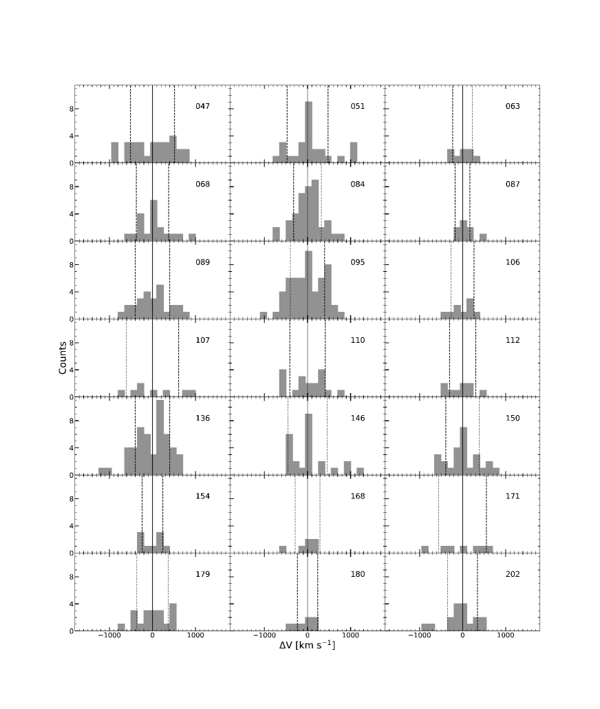
Figure 3: $\Delta V$ distributions for the spectroscopic cluster sub-sample. The [VMF98] cluster identification is included in each panel and our redshift estimates are shown with vertical solid lines and the velocity dispersions with dashed lines.

In order to improve the number of cluster members, we also selected galaxies without spectroscopic redshifts in the SDSS-DR13 using the $PHOTOZ$ table. We have selected galaxies with r${}_{p}\leq$ 1 Mpc, and $\Delta V\leq$ 10000 km s^-1 due to higher photometric redshift uncertainties. We divided the total redshift range in this study in three bins to have the same number of galaxy clusters in each one:

• z₁: $z\leq 0.065$;

• z₂: 0.065 $<$ z $<$ 0.10; and

• z₃: z $\geq$ 0.10.

To investigate the uncertainties and possible biases in the photometric redshifts, we have made a comparison of galaxies with both spectroscopic and photometric redshift estimates for each bin. Figure 4 shows the distributions of redshift differences between photometric ($z_{phot}$) and spectroscopic ($z$) redshifts in the three defined bins. Mean differences of $z_{phot}-z$ = 0.009 $\pm$ 0.014; 0.008 $\pm$ 0.013; and 0.002 $\pm$ 0.013 are also shown. The standard deviation of these values are around 0.01, which is equivalent to 6000 km s^-1 . Following Costa-Duarte et al. (2016), we have applied these differences to correct the photometric estimates to improve cluster membership. This result is also in agreement with the cluster definition of Nilo Castellón et al. (2016). Using this procedure, the photometric sub-sample has 45 galaxy clusters with more than 6 cluster members and the column (10) of the Table 1 quotes the number of photometric members.

Summarizing, we have two samples of cluster members: the spectroscopic sample and the total sample that includes both spectroscopic and photometric members. They are used to study the cluster RS and the LF in the three redshift bins.

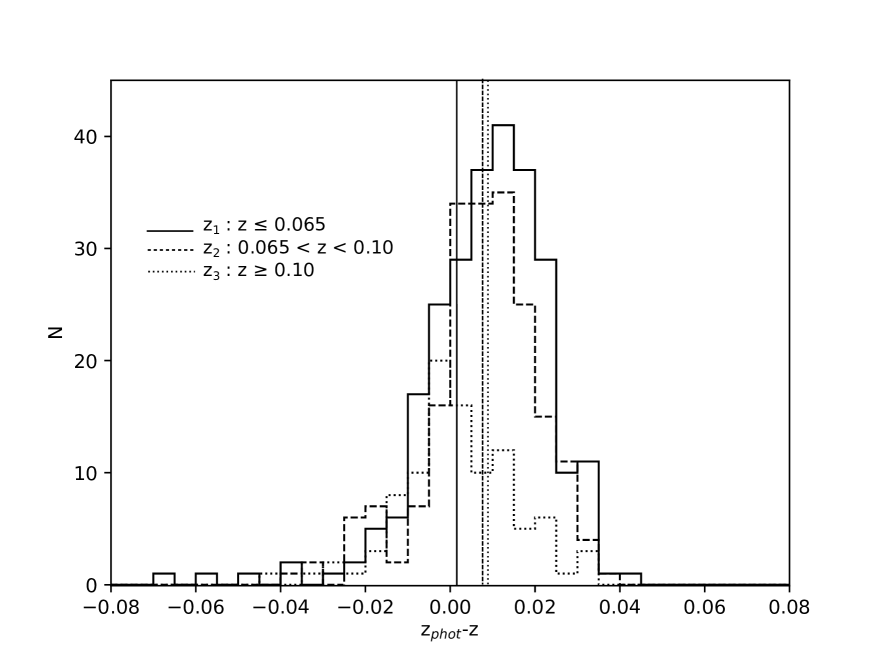
Figure 4: The redshift difference distributions between photometric and spectroscopic redshift estimates in the three bins. Vertical lines represent the mean differences. Both the distributions and mean differences are shown with different line types.

4 The Cluster Red Sequence

In the galaxy clusters, the early-type galaxies follow a well-defined relation in the Colour-Magnitude Diagrams extended by more than 4 magnitudes, the cluster Red Sequence (RS, Gladders et al. 1998; Gladders & Yee 2005).

In this work, we have considered absolute magnitudes of the galaxy cluster members and we have stacked all of them in the three redshift bins. Figure 5 shows the Colour-Magnitude Diagrams (M_g - M_r vs M_r) for the spectroscopic sub-sample of galaxy clusters in these bins. We have also computed the best spectroscopic RS linear fit in z₁ and z₂. In the case of the z₃ bin, we have fewer points only covering an interval of about -23 to -21 in M_r absolute magnitudes. For this reason, we have considered the RS fit obtained for z $<$ 0.1. Table 2 shows the three redshift bins in column (1); the best linear fit spectroscopic RS slopes and zero-points in columns (2) and (3), respectively; and the 1 $\sigma$ dispersion of the spectroscopic fits in column (4). In each panel of the figures, grey points are all spectroscopic members, the solid line represents the best spectroscopic RS linear fit quoted in the table and the two dash lines are the 1 $\sigma$ spectroscopic dispersions. Black points represent the cluster members that follow the spectroscopic RS fit within the dispersion. For z₁ and z₂, the RS slopes are similar.

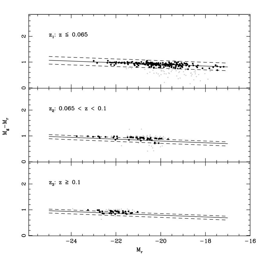
Figure 5: Colour-Magnitude Diagrams for spectroscopic members of the galaxy clusters in the three redshift bins. Grey points correspond to all spectroscopic members. Solid lines show the best spectroscopic RS fits and dashed lines, the 1 $\sigma$ spectroscopic dispersions. Black points represent the galaxies within 1 $\sigma$ dispersion of the spectroscopic RS fits.

We have also stacked the galaxy clusters using the photometric members. We have considered the RS fit obtained with the spectroscopic members because of the higher uncertainties in the photometric estimates. We have taken into account the spread of the photometric members relative to the spectroscopic RS fit and we have obtained the 1 $\sigma$ photometric dispersion, which is shown in the column (5) of the Table 2. Figure 6 shows the Colour-Magnitude Diagrams (M_g - M_r vs M_r) for the galaxy clusters with photometric members in the three redshift bins. Grey points represent these photometric members; solid lines, the spectroscopic RS fits (table 2) and the two dash lines, the 1 $\sigma$ photometric dispersions. Black points are the members that fit the spectroscopic RS within 1 $\sigma$ photometric dispersion. From the two figures we can see the passive galaxies that populate the inner parts of the galaxy clusters within 1$\sigma$ of the RS and below it, the forming galaxy population.

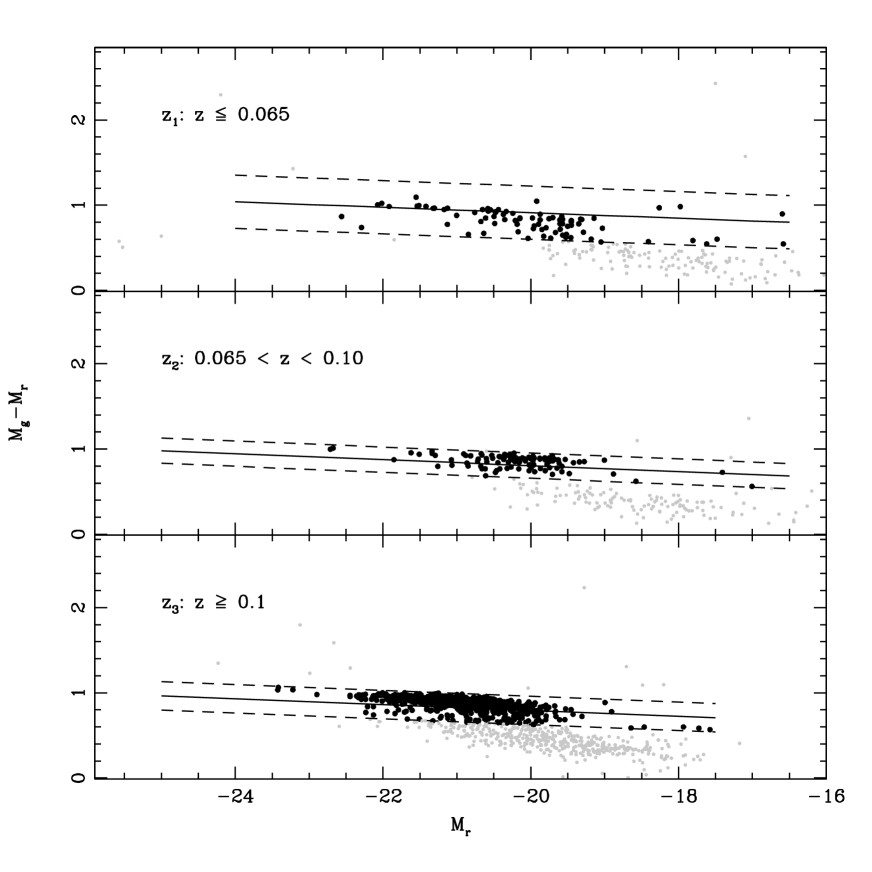
Figure 6: Colour-Magnitude Diagrams for photometric members of the galaxy clusters in the three redshift bins. Grey points correspond to all the photometric galaxies. Solid line shows the best spectroscopic RS fits and dashed lines are the 1 $\sigma$ photometric dispersion. Black points are the galaxies within 1 $\sigma$ photometric dispersion of the spectroscopic RS fits.

To analyse the photometric properties of these two populations, we have also used $C$, the galaxy concentration index. In the SDSS, this parameter is defined as the ratio of Petrossian radii that encloses 90 and 50 percent of the galaxy light (Stoughton et al. 2002). This quantity does not depend on distances and it is a suitable indicator of galaxy morphology (Strateva et al. 2001; Kauffmann et al. 2003a; Kauffmann et al. 2003b). Early-type galaxies have $C>2.55$ and late-type galaxies, $C<2.55$ (Strateva et al. 2001). We have obtained $C$ values in the $r-band$ for the total sample of members. Figure 7 shows the normalized $C$ distributions of these members in the three redshift bins. Solid histograms represent the distributions for galaxies within $1\sigma$ of the best spectroscopic RS fit and dash histograms, the distributions of those galaxies below the RS. The two $C$ distributions are different and we fit Gaussian functions to these two populations: early; and late types. Table 3 shows the mean $C$ values for the two populations in the different redshift bins. The mean $C$s are in agreement with the above definitions of galaxy types: about 2.7 for galaxies within $1\sigma$ the spectroscopic RS that correspond to early-type galaxies; and about 2.2 to late-types. At lower redshifts (z₁), the $C$ distribution of early-types is clear bimodal suggesting the presence of an intermediate galaxy population. Fitting two Gaussians we obtained $C$ = 2.50 $\pm$ 0.06 for this population. The results of the RSs and $C$ distributions suggest that in this work, we minimize the number of outliers in the sample of cluster members.

Figure 7: Normalized $C$ distributions for the total sample of members in the three redshift bins. Solid and dash histograms represent the distributions for members within $1\sigma$ of the spectroscopic RS fit and below it, respectively.

5 The galaxy luminosity function

The Schechter luminosity function (Schechter 1976) provides a parametric description of the space density of galaxies as a function of their luminosity. The form of this function is:

$$N(M)=0.4~{}ln(10)~{}\Phi^{*}(10^{0.4(M^{*}-M)})^{(\alpha+1)}exp(-10^{0.4(M^{*}-M)})$$

with M^∗, the characteristic absolute magnitude that corresponds to the ”knee” of the function; the slope $\alpha$ of the power law that dominates the faint-end; and $\phi^{*}$, the characteristic density. By using the cluster members, the computation of the cluster LF is straightforward without the need to obtain background galaxy determinations only requiring a correction for incompleteness.

The LF was obtained stacking the galaxy clusters in the three different redshift bins. We have computed the LF using the $1/V_{max}$ method considering the incompleteness with a $V/V_{max}$ test (Schmidt 1968). This method takes into account the volume of the survey enclosed by the galaxy redshift and the difference between the maximum and minimum volumes within which it can be observed. The value $\langle V/V_{max}\rangle$ varies with apparent magnitude. Considering a sample of sources uniformly distributed, we expect that half will be found in the inner half of the volume $V_{max}$ and the rest in the outer half. On average, we expect that $\langle V/V_{max}\rangle\sim 0.5$, and in this way, we can define the limiting magnitude where the catalogue is complete. In our case, we reached apparent magnitudes of $\sim 19.8$ mag in the $r-band$, which is a good compromise between the limiting magnitudes of both the spectroscopic and photometric samples. The LF errors were computed using the bootstrap re-sampling technique.

Figure 8 shows the stacked LF and errors for the three redshift bins using only spectroscopic members (left panels) and the total sample of members (right panels). Vertical lines represent the limiting magnitudes of the points considered in the Schechter fit. Solid lines represent the Schechter LF fit and the $M^{*}$ and $\alpha$ parameters of the fit are also shown in each panel. At lower redshifts, we can see that the LFs reach fainter magnitudes compared with the other two redshift bins. In general, the photometric members have a strong contribution at the LF faint-end in the three redshift bins. At higher redshifts, the number of spectroscopic members is smaller and they only contribute to the bright part. Including the photometric members allow us to extend the LF at the faint-end. Table 4 presents the three Schechter LF parameters in the studied redshift bins using spectroscopic members in columns (2) to (4); and with the full sample of members in columns (5) to (7).

Figure 8: Stacked Luminosity Functions in the three redsfhit bins. Left and right panels show the LFs obtained with only spectroscopic members and with the total sample of members, respectively. Vertical lines represent the limiting magnitudes beyond which the points were not considered in the Schechter fit and solid lines represent the best Schechter fit.

Our $M^{*}$ and $\alpha$ results are consistent with other authors using the SDSS data in the $r-band$. For instance, Zandivarez & Martínez (2011) obtained Schechter parameters for LFs in groups with mass ranging 12 $\leq$ $log({\cal M}/M_{\odot}$ h^-1) $\leq$ 15 up to redshifts of 0.2. Goto et al. (2002) converted parameters to this passband finding that $M^{*}$ ranges from -20.00 to -22.55 mag and $\alpha$ from -0.69 to -1.4 for different galaxy clusters (Valotto et al. 1997, Garilli et al. 1999 and Paolillo et al. 2000). Their estimates have higher uncertainties because they obtained the LF with only photometric data and they applied the statistical method for background subtraction. Our results of galaxy clusters with low X-ray luminosities are consistent with all these previous studies of groups and loose or poor galaxy clusters. The properties of these systems might be different but the parameters of the LFs are remarkably similar. This result suggests that the LF is a generic feature of the galaxy systems. In the redshift range of our study, the results are also in agreement with the study of Sarron et al. (2018) with SDSS galaxy clusters at z $<$ 0.7. They found similar $M^{*}$ and $\alpha$ parameters in their range of redshifts and masses.

6 Summary

This work is the forth in a series of papers aimed at understanding the processes involved in the formation and evolution of low X-ray luminosity galaxy clusters at intermediate redshifts.

The sample of spectroscopic members was defined with galaxies from the SDSS-DR13 that follow the criteria: r_p $\leq$ 1 Mpc and $\Delta V\leq\sigma$ using our $\sigma$ measurements. We have obtained a sub-sample of 21 galaxy clusters with more than 6 spectroscopic members. We have also defined a sample of photometric members with galaxies with r${}_{p}\leq$ 1 Mpc, and $\Delta V\leq$ 6000 km s^-1 . This photometric sub-sample has 45 galaxy clusters with more than 6 cluster members.

We have divided the redshift range in three bins: $z\leq 0.065$; 0.065 $<$ z $<$ 0.10; and z $\geq$ 0.10. We have stacked the galaxy clusters in the three redshift bins using the spectroscopic sub-sample and we have computed the best RS linear fit within 1$\sigma$ dispersion. With the photometric sub-sample we have added more data to the RS obtaining the photometric 1$\sigma$ dispersion relative to the spectroscopic RS fit. The $C$ distributions obtained with the members within 1$\sigma$ RS fit and below it have mean values of about 2.7 (early-type galaxies) and about 2.2 (late-type galaxies). These results are in agreement with the idea that early-type galaxies are the responsible of the tight RS relation.

We have also stacked the galaxy clusters in the three different redshift bins and computed the luminosity function using the $1/V_{max}$ method (Schmidt 1968). The Schechter parameters obtained for galaxy clusters with low X-ray luminosities are remarkably similar to other authors, in particular to groups and poor galaxy clusters at these lower redshifts.

We plan to extend this study to our complete sample of galaxy clusters at low X-ray luminosities in the redshift range 0.2 $<z<$ 0.7.

References

- Abazajian et al. (2009) Abazajian, K. N., Adelman-McCarthy, J. K., Agüeros, M. A., et al. 2009, ApJS, 182, 543
- Albareti et al. (2017) Albareti, F. D., Allende Prieto, C., Almeida, A., et al. 2017, ApJS, 233, 25
- Annunziatella et al. (2014) Annunziatella, M., Biviano, A., Mercurio, A., et al. 2014, A&A, 571, A80
- Baldry et al. (2004) Baldry, I. K., Balogh, M. L., Bower, R., Glazebrook, K., & Nichol, R. C. 2004, The New Cosmology: Conference on Strings and Cosmology, 743, 106
- Balogh et al. (2002) Balogh, M., Bower, R. G., Smail, I., et al. 2002, MNRAS, 337, 256
- Beers et al. (1990) Beers, T. C., Preston, G. W., Shectman, S. A., & Kage, J. A. 1990, AJ, 100, 849
- Biviano et al. (2013) Biviano, A., Rosati, P., Balestra, I., et al. 2013, A&A, 558, A1
- Boué et al. (2008) Boué, G., Adami, C., Durret, F., Mamon, G. A., & Cayatte, V. 2008, A&A, 479, 335
- Bower et al. (1992) Bower, R. G., Lucey, J. R., & Ellis, R. S. 1992, MNRAS, 254, 589
- Bower et al. (1992) Bower, R. G., Lucey, J. R., & Ellis, R. S. 1992, MNRAS, 254, 601
- Bower et al. (2006) Bower, R. G., Benson, A. J., Malbon, R., et al. 2006, MNRAS, 370, 645
- Christlein & Zabludoff (2003) Christlein, D., & Zabludoff, A. 2003, Ap&SS, 285, 197
- Collister et al. (2007) Collister, A., Lahav, O., Blake, C., et al. 2007, MNRAS, 375, 68
- Costa-Duarte et al. (2016) Costa-Duarte, M. V., O’Mill, A. L., Duplancic, F., Sodré, L., & Lambas, D. G. 2016, MNRAS, 459, 2539
- de Filippis et al. (2011) de Filippis, E., Paolillo, M., Longo, G., et al. 2011, MNRAS, 414, 2771
- Dekel & Silk (1986) Dekel, A., & Silk, J. 1986, ApJ, 303, 39
- de Lapparent (2003) de Lapparent, V. 2003, A&A, 408, 845
- De Lucia et al. (2004) De Lucia, G., Poggianti, B. M., Aragón-Salamanca, A., et al. 2004, ApJ, 610, L77
- De Lucia et al. (2010) De Lucia, G., Boylan-Kolchin, M., Benson, A. J., Fontanot, F., & Monaco, P. 2010, MNRAS, 406, 1533
- Doi et al. (2010) Doi, M., Tanaka, M., Fukugita, M., et al. 2010, AJ, 139, 1628
- Gaidos (1997) Gaidos, E. J. 1997, AJ, 113, 117
- Garilli et al. (1999) Garilli, B., Maccagni, D., & Andreon, S. 1999, A&A, 342, 408
- Gilbank & Balogh (2008) Gilbank, D. G., & Balogh, M. L. 2008, MNRAS, 385, L116
- Gladders et al. (1998) Gladders, M. D., López-Cruz, O., Yee, H. K. C., & Kodama, T. 1998, ApJ, 501, 571
- Gladders & Yee (2005) Gladders, M. D., & Yee, H. K. C. 2005, ApJS, 157, 1
- Gonzalez et al. (2015) Gonzalez, E. J., Foëx, G., Nilo Castellón, J. L., et al. 2015, MNRAS, 452, 2225
- Goto et al. (2002) Goto, T., Okamura, S., McKay, T. A., et al. 2002, PASJ, 54, 515
- Jenkins et al. (2001) Jenkins, A., Frenk, C. S., White, S. D. M., et al. 2001, MNRAS, 321, 372
- Kauffmann & Charlot (1998) Kauffmann, G., & Charlot, S. 1998, MNRAS, 294, 705
- Kauffmann et al. (2003a) Kauffmann, G., Heckman, T. M., White, S. D. M., et al. 2003a, MNRAS, 341, 33
- Kauffmann et al. (2003b) Kauffmann, G., Heckman, T. M., Tremonti, C., et al. 2003b, MNRAS, 346, 1055
- Klypin et al. (1999) Klypin, A., Gottlöber, S., Kravtsov, A. V., & Khokhlov, A. M. 1999, ApJ, 516, 530
- Lan et al. (2016) Lan, T.-W., Ménard, B., & Mo, H. 2016, MNRAS, 459, 3998
- Lerchster et al. (2011) Lerchster, M., Seitz, S., Brimioulle, F., et al. 2011, MNRAS, 411, 2667
- Lopez-Cruz (1997) Lopez-Cruz, O. 1997, Ph.D. Thesis, 2803
- McGee et al. (2009) McGee, S. L., Balogh, M. L., Bower, R. G., Font, A. S., & McCarthy, I. G. 2009, MNRAS, 400, 937
- Moore & Ridge (1999) Moore, T., & Ridge, N. 1999, Star Formation 1999, 293
- Mullis et al. (2003) Mullis, C. R., McNamara, B. R., Quintana, H., et al. 2003, ApJ, 594, 154