On the Finite Time Blowup of the De Gregorio Model for the 3D Euler Equations

Abstract.

We present a novel method of analysis and prove finite time asymptotically self-similar blowup of the De Gregorio model [12, 13] for some smooth initial data on the real line with compact support. We also prove self-similar blowup results for the generalized De Gregorio model [40] for the entire range of parameter on $\mathbb{R}$ or $S^{1}$ for Hölder continuous initial data with compact support. Our strategy is to reformulate the problem of proving finite time asymptotically self-similar singularity into the problem of establishing the nonlinear stability of an approximate self-similar profile with a small residual error using the dynamic rescaling equation. We use the energy method with appropriate singular weight functions to extract the damping effect from the linearized operator around the approximate self-similar profile and take into account cancellation among various nonlocal terms to establish stability analysis. We remark that our analysis does not rule out the possibility that the original De Gregorio model is well posed for smooth initial data on a circle. The method of analysis presented in this paper provides a promising new framework to analyze finite time singularity of nonlinear nonlocal systems of partial differential equations.

1. Introduction

In the absence of external forcing, the three-dimensional Navier-Stokes equations for incompressible fluid read:

(1.1) $$\mathbf{u}_{t}+\mathbf{u}\cdot\nabla\mathbf{u}=-\nabla p+\nu\Delta\mathbf{u},\quad\nabla\cdot\mathbf{u}=0.$$

Here $\mathbf{u}(x,t):\mathbb{R}^{3}\times[0,T)\to\mathbb{R}^{3}$ is the 3D velocity vector of the fluid, and $p(x,t):\mathbb{R}^{3}\times[0,T)\to\mathbb{R}$ describes the scalar pressure. The viscous term $\nu\Delta\mathbf{u}$ models the viscous forcing in the fluid. In the case of $\nu=0$, equations (1.1) are referred to as the Euler equations. The divergence-free condition $\nabla\cdot\mathbf{u}=0$ enforces the incompressibility of the fluid. The Navier-Stokes equations are among the most fundamental nonlinear partial differential equations. The fundamental question regarding the global regularity of the 3D Euler and Navier-Stokes equations for general smooth initial data with finite energy remains open, and it is generally viewed as one of the most important open questions in mathematical fluid mechanics, see the surveys [17, 32, 9, 18, 21].

Define vorticity ${\boldsymbol{\omega}}=\nabla\times{\bf u}$, then ${\boldsymbol{\omega}}$ is governed by

(1.2) $${\boldsymbol{\omega}}_{t}+({\bf u}\cdot\nabla){\boldsymbol{\omega}}=\nabla{\bf u}\cdot{\boldsymbol{\omega}}+\nu\Delta{\boldsymbol{\omega}}.$$

The term $\nabla{\bf u}\cdot{\boldsymbol{\omega}}$ on the right hand side is referred to as the vortex stretching term, which is absent in the two dimensional case. Note that $\nabla{\bf u}$ is formally of the same order as ${\boldsymbol{\omega}}$. In fact, if ${\bf u}$ decays sufficiently fast in the far field, one can show that $c_{p}\|{\boldsymbol{\omega}}\|_{L^{p}}\leq\|\nabla{\bf u}\|_{L^{p}}\leq C_{p}\|{\boldsymbol{\omega}}\|_{L^{p}}$ for $1<p<\infty$ with constants $c_{p},C_{p}>0$ depending on $p$. Thus the vortex stretching term scales quadratically as a function of vorticity, i.e. $\nabla{\bf u}\cdot{\boldsymbol{\omega}}\approx{\boldsymbol{\omega}}^{2}$. The vortex stretching term in the 3D Navier-Stokes or Euler equations is the main source of difficulty in obtaining global regularity.

1.1. The De Gregorio model and its variant

In this paper, we study the finite time singularity of the 1D De Gregorio model [12, 13] and its generalization. The De Gregorio model is a simplified model to study the effect of advection and vortex stretching in the 3D incompressible Euler equations. Specifically, the inviscid De Gregorio model is given below

(1.3) $$\omega_{t}+au\omega_{x}=u_{x}\omega\;,\quad u_{x}=H\omega\;,$$

where $H$ is the Hilbert transform and $a\in\mathbb{R}$ is a parameter. In this 1D model, $\omega$ models the vorticity ${\boldsymbol{\omega}}$ in the 3D Euler equations (1.2) with $\nu=0$. The nonlinear terms $u\omega_{x}$ and $u_{x}\omega$ model the advection term $({\bf u}\cdot\nabla){\boldsymbol{\omega}}$ and the vortex stretching term $\nabla{\bf u}\cdot{\boldsymbol{\omega}}$, respectively. The Biot-Savart law is modeled by $u_{x}=H\omega$, which preserves the same scaling as that of the original Biot-Savart law. The case of $a=0$ is reduced to the well-known Constantin-Lax-Majda model [10], in which the authors proved the finite time singularity formation for a class of smooth initial data. The case of $a=1$ was proposed by De Gregorio in [12] and its generalization to $a\in\mathbb{R}$ was proposed by Okamoto et. al. in [40]. Throughout this paper, we call equation (1.3) the De Gregorio (DG) model. There are various 1D models proposed in the literature. We refer to [16, 27] for excellent surveys of other 1D models for the 3D Euler equations and the surface quasi-geostrophic equation.

One important feature of the De Gregorio model is that it captures the competition between the advection term and the vortex stretching term. It is not hard to see that when $a<0$, the advection effect would work together with the vortex stretching effect to produce a singularity. Indeed, Castro and Córdoba [1] proved the finite time blow-up for $a<0$ based on a Lyapunov functional argument. For $a>0$, there are competing nonlocal stabilizing effect due to the advection and the destabilizing effect due to vortex stretching, which are of the same order in terms of scaling. Even for arbitrarily small $a>0$, in which case we expect that the advection effect is much weaker than the vortex stretching, using the same Lyapunov functional argument in [1] would fail to prove a finite time singularity since the control of the solution through the Lyapunov functional is not strong enough. We remark that the stabilizing effect of advection has also been studied by Hou-Li in [23] for an exact 1D model of the 3D axisymmetric Navier-Stokes equations along the symmetry axis and by Hou-Lei for a 3D model of the axisymmetric Navier-Stokes equations in [22].

The question of whether the De Gregorio model would develop a finite time singularity for $a>0$ has remained unsolved for some time, especially in the case of $a=1$. In a recent paper by Elgindi and Jeong [16], they constructed a smooth self-similar profile for small $|a|$ and a $C^{\alpha}$ self-similar profile for all $a\in\mathbb{R}$ using a power series expansion and an iterative construction. We note that the self-similar profiles constructed in [16] decay slowly in the far field and the corresponding velocity $u$ does not have finite energy. In [34], Castro performed some preliminary study on (1.3) with $a=1$ both analytically and numerically and obtained finite time blowup from $C_{c}^{\infty}$ initial data under some convexity and monotonicity assumptions on the solution.

1.2. Main results

Let $\Omega,c_{l},c_{\omega}$ be the solution of the self-similar equation of (1.3) given below

(1.4) $$(c_{l}x+aU)\Omega_{x}=(c_{\omega}+U_{x})\Omega,\quad U_{x}=H\Omega,$$

with $c_{\omega}<0$ and a self-similar profile $\Omega\neq 0$ in some weighted $H^{1}$ space. Then for some given $T>0$,

(1.5) $$\omega(x,t)=\frac{1}{(T-t)|c_{\omega}|}\Omega\left(\frac{x}{(T-t)^{\gamma}}\right),\quad\gamma=-\frac{c_{l}}{c_{\omega}},$$

is a self-similar singular solution of (1.3).

We define some notions about the self-similar singularities to be used in this paper.

Definition 1.1 (Two types of asymptotically self-similar singularities).

We say that a singular solution $\omega$ of (1.3) is asymptotically self-similar if there exists a solution of (1.4) $(\Omega,c_{l},c_{\omega})$ with $\Omega\neq 0$ in some weighted $H^{1}$ space and $c_{\omega}<0$ such that the following statement holds true. By rescaling $\omega$ dynamically, i.e. $C_{\omega}(t)\omega(C_{l}(t)x,t)$ for some time dependent scaling factors $C_{\omega}(t),C_{l}(t)>0$, it converges to $\Omega$ as $t\to T^{-}$ in some weighted $L^{2}$ norm, where $T>0$ is the blowup time. In addition, we say that the asymptotically self-similar singularity is of the expanding type if the self-similar solution (1.5) associated to $(\Omega,c_{l},c_{\omega})$ satisfies $\gamma<0$ and of the focusing type if $\gamma>0$. We call $\gamma$ the scaling exponent.

Remark 1.2.

We will specify in later Sections the weighted $L^{2}$ norm in which the dynamically rescaled function of $\omega$ converges to the self-similar profile $\Omega$ in the following Theorems. We will also specify in later Sections the stronger weighted $H^{1}$ norm that the self-similar profile $\Omega$ belongs to, so that the Hilbert transform $U_{x}=H\Omega$ is well defined and $(\Omega,c_{l},c_{\omega})$ is a solution of (1.4). In the case of small $|a|$, we refer to Propositions 3.1, 3.2 and Section 3.3 for more precise statements. Similar statements also apply to other cases.

Our first main result is regarding the finite time singularity of the original De Gregorio model.

Theorem 1.

There exist some $C_{c}^{\infty}$ initial data on $\mathbb{R}$ such that the solution of (1.3) with $a=1$ develops an expanding and asymptotically self-similar singularity in finite time with scaling exponent $\gamma=-1$ and compactly supported self-similar profile $\Omega\in H^{1}(\mathbb{R})$.

Although the initial data and the self-similar profile $\Omega$ have compact support, due to the expanding nature of the blowup, the support of the solution will become unbounded at the blowup time.

Remark 1.3.

Surprisingly, the blowup solution in Theorem 1 satisfies the property that $||\omega(x,t)/x||_{L^{\infty}}$ is uniformly bounded up to the blowup time, $\sup_{t\in[0,T)}||\omega(x,t)/x||_{\infty}<+\infty$, which can be seen from the special scaling exponent $\gamma=-1$ and the proof of Theorem 1.

Remark 1.4.

The uniform boundedness of $||\omega(t)/x||_{L^{\infty}}$ over $[0,T)$ implies that $\omega(x,t)$ cannot blowup at any finite $x$, which is consistent with the expanding nature of the blowup.

The second result is finite time blowup of (1.3) for small $|a|$ with $C_{c}^{\infty}$ initial data.

Theorem 2.

There exists a positive constant $\delta>0$ such that for $|a|<\delta$, the solution of (1.3) with some $C_{c}^{\infty}$ initial data develops a focusing and asymptotically self-similar singularity in finite time with self-similar profile $\Omega\in H^{1}(\mathbb{R})$.

The third result is finite time blowup of (1.3) for all $a$ with $C_{c}^{\alpha}$ initial data.

Theorem 3.

There exists $C_{1}>0$ such that for $0<\alpha<\min(1/4,\;C_{1}/|a|)$, the solution of (1.3) with some $C_{c}^{\alpha}$ initial data develops a focusing and asymptotically self-similar singularity in finite time with self-similar profile $\Omega$ satisfying $|x|^{-1/2}\Omega\in L^{2}$ and $|x|^{1/2}\Omega_{x}\in L^{2}$.

The blowup results in Theorem 2 and Theorem 3 also hold for the De Gregorio model on the circle.

Theorem 4.

Consider (1.3) on the circle. (1) There exists $C_{1}>0$ such that if $|a|<C_{1}$, the solution of (1.3) develops a singularity in finite time for some $C_{c}^{\infty}$ initial data. (2) If $0<\alpha<\min(1/4,\;C_{1}/|a|)$, then the solution of (1.3) develops a finite time singularity for some initial data $\omega_{0}\in C^{\alpha}$ with compact support.

Remark 1.5.

Due to the fact that (1.3) on a circle does not enjoy the perfect spatial scaling symmetry, we do not establish the result on the asymptotically self-similar singularity in the above theorem.

The initial data $\omega_{0}$ we constructed for the previous theorems all satisfy the property that $\omega_{0}$ is odd and $\omega_{0}\leq 0$ for $x>0$. The following theorem implies that for $a>0$, the Hölder regularity for $\omega_{0}$ in this class is crucial for the focusing self-similar blow-up.

Theorem 5.

There exists a universal positive constant $a_{0}$ such that the following statement holds true. Suppose that $a>0,1\geq\alpha>a_{0}/a$, and $\omega_{0}\in C^{\alpha}$ is odd, non-positive for $x>0$ and has compact support. Then the solution of (1.3) with initial data $\omega_{0}$ cannot develop an asymptotically self-similar singularity with blowup scaling $c_{l}>-\alpha^{-1}$ in finite time. In particular, the solution of (1.3) with initial data $\omega_{0}$ cannot develop a focusing and asymptotically self-similar singularity in finite time.

Theorem 3 and Theorem 5 show that the critical Hölder exponent of the initial data for a finite time, focusing and asymptotically self-similar singularity is $\alpha\approx\frac{1}{a}$ for large positive $a$. For (1.3) on the circle, we can prove stronger results. See Theorem 6 and Proposition 5.11 in Section 5.3.2. In particular, for a class of initial data $\omega_{0}$ that vanishes to the order $|x|^{\kappa}$ near $x=0$ with $\kappa$ larger than certain threshold, we show that $u_{x}(0,t)$ cannot blow up at the first singularity time $T$ if it exists. In contrast, $u_{x}(0,t)$ actually blows up at the first singularity time for the blowup solution that we construct in Theorem 4.

Recently, the first author established finite time blowup of (1.3) on the circle with $1-\delta<a<1$ from smooth initial data for some $\delta>0$ in [5]. This resolves the endpoint case of the conjecture made in [16, 41] that equation (1.3) develops a finite time singularity for $a<1$ from smooth initial data in the case of a circle. We remark that Theorems 1, 4 and the result in [5] do not rule out the possibility that the De Gregorio model (1.3) with $a=1$ is globally well-posed for smooth initial data on the circle. In a recent paper by Jia, Stewart and Sverak [25], they studied the De Gregorio model with $a=1$ on a circle and proved the nonlinear stability of the equilibrium $A\sin(2(\theta-\theta_{0}))$ of (1.3) for periodic solutions with period $\pi$. In [29], Lei, Liu and Ren proved global well-posedness of the solution of (1.3) with $a=1$ on the real line or a circle for initial data $\omega_{0}$ that does not change sign and $|\omega_{0}|^{1/2}\in H^{1}(S^{1})$. These results shed useful light on the DG model on $S^{1}$ for smooth solutions.

We remark that an important observation made by Elgindi and Jeong in [16] is that the advection term can be substantially weakened by choosing $C^{\alpha}$ data with small $\alpha$. We use this property in the proof of Theorem 3. After we completed our work, we learned from Dr. Elgindi that results similar to Theorems 2 and 3 have recently been established independently by Elgindi, Ghoul and Masmoudi [15] on the asymptotically self-similar solutions of (1.3) with finite energy and the stability of the asymptotically self-similar blowup.

1.3. A novel method of analysis

One of the main contributions of this paper is that we introduce a novel method of analysis that enables us to prove finite time singularity for the original De Gregorio model with $C_{c}^{\infty}$ initial data. Our method of analysis consists of several steps. The first step is to construct an approximate self-similar profile for the De Gregorio model with a small residual error in some energy norm. The second step is to perform linear stability analysis around this approximate self-similar profile in the dynamic rescaling equation with some appropriately chosen normalization conditions and energy norm. The third step is to establish nonlinear stability using a bootstrap argument. See Section 2 for more details on these steps.

Finally, we choose an initial perturbation sufficiently small in the energy norm so that the initial condition of the De Gregorio model has compact support and show that the solution develops a singularity in finite time. Moreover, we prove that the solution of the dynamic rescaling equation converges to the exact self-similar solution exponentially fast in time in the weighted $L^{2}$ norm. This enables us to show that by rescaling the solution of (1.3) dynamically, it converges to the exact self-similar profile at the blowup time in the weighted $L^{2}$ norm and the singularity is asymptotically self-similar.

The method of analysis presented in this paper provides a promising new framework to analyze potential finite time singularity of a nonlinear and nonlocal system of partial differential equations. We have been able to generalize this method of analysis in several aspects. The first author of this paper has generalized this framework to prove finite time asymptotically self-similar blowup of (1.3) with dissipation for certain range of $a$ in [6]. We have also established finite time self-similar blowup of the HL model proposed in [24, 31] with $C_{c}^{\infty}$ initial data (see also a recent paper in [8]). Recently the first two authors of this paper have been able to generalize this framework to prove finite time blowup of the 2D Boussinesq and 3D axisymmetric Euler equations with $C^{1,\alpha}$ velocity and boundary in [7], which share the same symmetry and sign property as the Luo-Hou scenario [31, 30]. The analysis of the HL model, 2D Boussinesq equations or the 3D Euler equations is much more challenging than that of the De Gregorio model since it is a nonlinear nonlocal system. We are currently working to extend our method of analysis to prove the finite time blowup of the 2D Boussinesq system with smooth initial data.

Organization of the paper

In Section 2, we outline our general strategy that we use to prove nonlinear stability for various cases. In Section 3, we study the De Gregorio model with small $|a|$. In Section 4, we construct an approximate self-similar profile with a small residual error numerically for the case of $a=1$ and apply our method of analysis to prove the finite time self-similar blowup for $C_{c}^{\infty}$ initial data. In Section 5, we study the case with any $a\in\mathbb{R}$ and prove finite time singularity for any $a\in\mathbb{R}$ on both $\mathbb{R}$ and $S^{1}$ for some $C^{\alpha}$ initial data with compact support. Finally, in Section 6, we use a Lyapunov functional argument to prove finite time blowup for all $a<0$ with smooth initial data. In the Appendix, we prove several useful properties of the Hilbert transform and some functional inequalities.

Notations

Since the functions that we consider in this paper, e.g. $\omega,u$, have odd or even symmetry, we just need to consider $R^{+}$. The inner product is defined on $R^{+}$, i.e.

$$\langle f,g\rangle\triangleq\int_{0}^{\infty}fgdx,\quad||f||_{L^{p}}\triangleq\left(\int_{0}^{\infty}|f|^{p}dx\right)^{1/p}.$$

In Section 4, we further restrict the inner product and the norm to the interval $[0,L]$, e.g $\langle f,g\rangle=\int_{0}^{L}fgdx$, since the support of $\omega,\bar{\omega}$ lies in $[-L,L]$.

We use $C,C_{i}$ to denote absolute constants and $C(A,B,..,Z)$ to denote constant depending on $A,B,..,Z$. These constants may vary from line to line, unless specified. We also use the notation $A\lesssim B$ if there is some absolute constant $C$ such that $A\leq CB$, and denote $A\asymp B$ if $A\lesssim B$ and $B\lesssim A$. We use $\rightarrow$ to denote strong convergence and $\rightharpoonup$ to denote weak convergence in some norm. The upper bar notation is reserved for the approximate profile, e.g. $\bar{\omega}$. The letters $e,f,a_{1},a_{2},a_{3}$ are reserved for some parameters that we will choose in Section 4.

2. Outline of the general strategy in establishing nonlinear stability

Our general strategy in establishing nonlinear stability is to first construct an approximate self-similar profile with a small residual error for the De Gregorio model (1.3), then prove linear and nonlinear stability of this profile in the dynamic rescaling equation (see equation (2.1) below). We use both analytic and numerical approaches to construct the approximate self-similar profile in various cases. The analytic approach is based on a class of self-similar profiles of the Constantin-Lax-Majda model (CLM) [10], or equivalent (1.3) with $a=0$, which are derived in [16]. In [16], the exact self-similar profiles of (1.3) with $a\neq 0$ are also constructed in various cases. We remark that our analysis does not rely on these profiles of (1.3) with $a\neq 0$.

In general, it is very difficult to construct a self-similar profile analytically. An important observation is that the self-similar profile is equivalent to the steady state of the dynamic rescaling equation. If we can solve the dynamic rescaling equation for long enough time numerically to obtain an approximate steady state with a small residual error, this will give an approximate self-similar profile. Due to this connection, we will not distinguish the approximate steady state of the dynamic rescaling equation and the approximate self-similar profile of the De Gregorio model throughout this paper. We will use this approach to obtain a piecewise smooth approximate self-similar profile $\bar{\omega}$ with a small residual error for (1.3) in the case of $a=1$.

A very essential part of our analysis is to prove linear and nonlinear stability of the approximate steady state of the dynamic rescaling equation. The dynamic rescaling equation of (1.3) is given below

(2.1) $$\omega_{t}+(c_{l}(t)x+au)\omega_{x}=(c_{\omega}(t)+u_{x})\omega\;,$$

where $c_{l}(t)$ and $c_{\omega}(t)$ are time-dependent scaling parameters. See (3.1)-(3.3) in subsection 3.1 for more discussion on the dynamic rescaling formulation. Let $(\bar{\omega},\bar{u},\bar{c_{l}},\bar{c_{\omega}})$ be an approximate steady state of the dynamic rescaling equation. We define the linearized operator $L(\omega)$

(2.2) $$L(\omega)=-(\bar{c}_{l}x+a\bar{u})\omega_{x}+(\bar{c}_{\omega}+\bar{u}_{x})\omega+(u_{x}+c_{\omega})\bar{\omega}-(au+c_{l}x)\bar{\omega}_{x},\quad u_{x}=H\omega,$$

where the scaling factors $c_{l}$ and $c_{\omega}$, which depend on $\omega$, will be chosen later. Let $\omega$ be the perturbation around the approximate steady state $\bar{\omega}$. The stability around $\bar{\omega}$ is reduced to analyzing the nonlinear stability of the dynamic equation

(2.3) $$\omega_{t}=L(\omega)+N(\omega)+F$$

around $\omega=0$. The perturbation $\omega$ lies in $\mathcal{H}(\Omega)$, a Hilbert space on a domain $\Omega$. Here $F=(\bar{c}_{\omega}+\bar{u}_{x})\bar{\omega}-(\bar{c_{l}}x+a\bar{u})\bar{\omega}_{x}$ is the residual error and $N(\omega)=(c_{\omega}+u_{x})\omega-(c_{l}x+u)\omega_{x}$ is the non-linear operator. We remark that $L(\omega)$ and $N(\omega)$ are nonlocal operators since $u_{x}=H(\omega)$ is nonlocal. Due to the presence of the non-linear operator $N$ and the error term $F$, it is not sufficient to only show that the spectrum of $L$ has negative real parts.

Our approach is to first perform the weighted $L^{2}$ estimate with appropriate weight function $\varphi$ to establish the linear stability (we drop the terms $N(\omega)$ and $F$ to illustrate the main ideas)

(2.4) $$\frac{1}{2}\frac{d}{dt}\langle\varphi\omega,\omega\rangle=\langle\varphi\omega,L(\omega)\rangle\leq-\lambda\langle\varphi\omega,\omega\rangle,\quad\omega\in\mathcal{H}(\Omega)$$

for some $\lambda>0$ and then extend the above estimates to the weighted $H^{1}$ estimates. We can use a bootstrap argument to establish the nonlinear stability of (2.3), provided that $F$ is sufficiently small in the energy norm.

We will focus on the linear stability (2.4) to illustrate the main ideas. The linearized equation around some approximate self-similar profile $(\bar{\omega},\bar{u},\bar{c}_{l},\bar{c}_{\omega})$ reads

$$\omega_{t}=-(\bar{c}_{l}x+a\bar{u})\omega_{x}+(\bar{c}_{\omega}+\bar{u}_{x})\omega+(u_{x}+c_{\omega})\bar{\omega}-(au+c_{l}x)\bar{\omega}_{x}\;.$$

The linear stability of the profile is mainly due to the damping effect from some local terms and cancellation among several nonlocal terms.

2.1. Derivation of the damping term

The damping effect of the equation comes from two parts that depend locally on $\omega$: the stretching term $(\bar{c}_{l}x+a\bar{u})\omega_{x}$ and the vortex stretching term $(\bar{c}_{\omega}+\bar{u}_{x})\omega$. An important observation of the approximate profile is that $(\bar{c}_{\omega}+\bar{u}_{x})$ is negative for large $|x|$, thus the vortex stretching term $(\bar{c}_{\omega}+\bar{u}_{x})\omega$ is a damping term for large $|x|$. This is the main source of the damping effect for large $|x|$. However, $(\bar{c}_{\omega}+\bar{u}_{x})\omega$ is not a damping term for $x$ near $0$ since $\bar{c}_{\omega}+\bar{u}_{x}$ is positive.

For $x$ close to $0$, we choose a singular weight $x^{-k},k\in\mathbb{N}_{+}$ to take advantage of the stretching term. Performing the weighted $L^{2}$ estimate, we get

(2.5) $$\frac{1}{2}\frac{d}{dt}\langle\omega^{2},x^{-k}\rangle =\langle-(\bar{c}_{l}x+a\bar{u})\omega_{x}+(\bar{c}_{\omega}+\bar{u}_{x})\omega,\omega x^{-k}\rangle$$

$$+\langle(u_{x}+c_{\omega})\bar{\omega}-(au+c_{l}x)\bar{\omega}_{x},\omega x^{-k}\rangle\triangleq I+II.$$

The profile we constructed satisfies $\bar{c}_{l}x+a\bar{u}>0$ for all $x>0$ and $\bar{c}_{l}x+a\bar{u}\approx Cx$ near $x=0$ for some $C>0$, which can be seen in later sections. Hence, we make a simplified assumption that $\bar{c}_{l}x+a\bar{u}=Cx$ for some $C>0$ to illustrate the idea. Using integration by parts, we obtain

$$I=\Big{\langle}-\frac{C(k-1)}{2}+(\bar{c}_{\omega}+\bar{u}_{x}),\omega^{2}x^{-k}\Big{\rangle}\triangleq\langle D,\omega^{2}x^{-k}\rangle\;.$$

We will choose $k$ so that the coefficient $D$ is negative (we choose $k=4$ for $a=1$ and small $|a|$). In our analysis, the main damping term for $x$ near $0$ is obtained from $(\bar{c}_{l}x+a\bar{u})\omega_{x}$. In addition, for large $|x|$, under the assumption $(\bar{c}_{l}x+a\bar{u})\omega_{x}=Cx\omega_{x}$, we can obtain a damping term from $(\bar{c}_{l}x+a\bar{u})\omega_{x}$ in the $L^{2}(x^{-k})$ energy estimate after performing integration by parts provided that $k-1>0$. In this case, the weight $x^{-k}$ decays faster than $x^{-1}$. Similar analysis and results also hold for $(\bar{c}_{l}x+a\bar{u})\omega_{x}$ in the range of large $|x|$ without assuming $\bar{c}_{l}x+a\bar{u}=Cx$ for all $x$ and some $C>0$. In order to control the perturbation $\omega$ in the far field, we have to choose a weight $\varphi$ that decays more slowly than $x^{-1}$ so that the weighted $L^{2}$ norm of $\omega$ is not too weak for large $|x|$. As a result, $(\bar{c}_{l}x+a\bar{u})\omega_{x}$ does not produce a damping term for large $|x|$ in our weighted $L^{2}$ estimate after performing integration by parts. This is one of the subtleties in our analysis.

The above derivations also apply to the case of $a=1$, where the approximate steady state $\bar{\omega}$ and the perturbation $\omega$ have finite support $[-L,L]$. The damping term near $x=0$ is mainly from $(\bar{c}_{l}x+\bar{u})\omega_{x}$, while the damping term near $x=\pm L$ is mainly from $(\bar{c}_{\omega}+\bar{u}_{x})\omega$.

Another subtlety in our analysis is that we do not use a singular weight to derive a damping term from $(\bar{c}_{l}x+\bar{u})\omega_{x}$ in all cases with different $a$. In the case of $a=1$, we need to estimate the perturbation near the endpoints $x=0,\pm L$ carefully. We choose a singular weight $\varphi$ of order $O((x-L)^{-2})$ near $x=L$ in order to obtain a sharp estimate of $u$. See more discussions in next Section.

2.2. Estimates of the nonlocal terms

The II term in (2.5) consists of several nonlocal terms that are difficult to control. To estimate the vortex stretching term $(u_{x}+c_{\omega})\bar{\omega}$ in (2.5), we take full advantage of the cancellation between $u_{x}$ and $\omega$, see Lemmas A.3 and A.4. To control the last term $-(au+c_{l}x)\bar{\omega}_{x}$ in (2.5), we have to choose appropriate functional spaces $(X,Y)$ and develop several functional inequalities $||u||_{X}\leq C_{XY}||\omega||_{Y}$ with a sharp constant $C_{XY}$. For example, we need to make use of the isometry property of the Hilbert transform. We remark that an overestimate of the constant $C_{XY}$ could lead to the failure of the linear stability analysis since the effect of the advection term can be overestimated. To implement the above ideas in obtaining the damping term and estimating the nonlocal terms, we need to design the singular weight very carefully. See (3.6) and (4.6) for some singular weights that are used in our analysis.

We remark that some weighted Sobolev spaces with singular weights have been used in [29, 25] for the nonlinear stability analysis of the steady state of (1.3) with $a=1$ on the circle. Singular weights similar to those in Sections 3, 5 and in the form of linear combination of $|x|^{-k}$ have also been designed independently in [14, 15] for the stability analysis.

2.3. Energy estimates with computer assistance

In the case of $a=1$, we use computer-assisted analysis in the following aspects. As we discuss at the beginning of Section 2, we construct the approximate self-similar profile numerically. We use numerical analysis with rigorous error control to verify that the residual error is small in the energy norm. The key part of the stability analysis is to use energy estimates to establish the linear stability. In the energy estimates, instead of bounding several coefficients by some absolute constants, which leads to overestimates, we keep track of these coefficients. Since these coefficients depend on the approximate self-similar profile constructed numerically, we use numerical computation with rigorous error control to verify several inequalities that involve these coefficients. See Sections 4.1, 4.3 and 4.4.1 for more discussions.

There is another computer-assisted approach to establish the stability by tracking the spectrum of a given operator and quantifying the spectral gap; see, e.g. [2]. The key difference between this approach and our approach is that we do not use computation to quantify the spectral gap of the linearized operator $L$ in (2.2). In fact, the linearized operator $L$ is not a compact operator due to the Hilbert transform $u_{x}=H\omega$ and the non-compact part of $L$ cannot be treated as a small perturbation. Thus we cannot approximate the linearized operator by a finite rank operator which can be estimated using numerical computation. We refer to [19] for an excellent survey of other computer assisted proofs in PDE.

3. Finite Time Self-Similar Blowup for Small $|a|$

In this section, we will present the proof of Theorem 2. We use this example to illustrate the main ideas in our method of analysis by carrying stability analysis around an approximate self-similar profile with a small residual error by using a dynamic rescaling formulation. In this case, we have an analytic expression for the approximate steady state $\bar{\omega}$.

3.1. Dynamic rescaling formulation

We will prove Theorem 2 by using a dynamic rescaling formulation. Let $\omega(x,t),u(x,t)$ be the solutions of the original equation (1.3), then it is easy to show that

(3.1) $$\tilde{\omega}(x,\tau)=C_{\omega}(\tau)\omega(C_{l}(\tau)x,t(\tau)),\quad\tilde{u}(x,\tau)=C_{\omega}(\tau)C_{l}(\tau)^{-1}u(C_{l}(\tau)x,t(\tau))$$

are the solutions to the dynamic rescaling equations

(3.2) $$\tilde{\omega}_{\tau}(x,\tau)+(c_{l}(\tau)x+a\tilde{u})\tilde{\omega}_{x}(x,\tau) =c_{\omega}(\tau)\tilde{\omega}+\tilde{u}_{x}\omega\quad\tilde{u}_{x} =H\tilde{\omega},$$

where

(3.3) $$C_{\omega}(\tau)=\exp\left(\int_{0}^{\tau}c_{\omega}(s)d\tau\right),\ C_{l}(\tau)=\exp\left(\int_{0}^{\tau}-c_{l}(s)ds\right),\ t(\tau)=\int_{0}^{\tau}C_{\omega}(\tau)d\tau\;.$$

We have the freedom to choose the time-dependent scaling parameters $c_{l}(\tau)$ and $c_{\omega}(\tau)$ according to some normalization conditions. After we determine the normalization conditions for $c_{l}(\tau)$ and $c_{\omega}(\tau)$, the dynamic rescaling equation is completely determined and the solution of the dynamic rescaling equation is equivalent to that of the original equation using the scaling relationship described in (3.1)-(3.3), as long as $c_{l}(\tau)$ and $c_{\omega}(\tau)$ remain finite. We remark that the dynamic rescaling formulation was introduced in [35, 28] to study the self-similar blowup of the nonlinear Schrödinger equations. This formulation is also called the modulation technique in the literature and has been developed by Merle, Raphael, Martel, Zaag and others. It has been a very effective tool to analyze the formation of singularities for many problems like the nonlinear Schrödinger equation [26, 36], the nonlinear wave equation [38], the nonlinear heat equation [37], the generalized KdV equation [33], and other dispersive problems.

If there exist $C,c>0$ such that for any $\tau>0$, $c_{\omega}(\tau)\leq-C<0$ and $|\tilde{\omega}|$ is bounded from below $||\tilde{\omega}(\cdot,\tau)||_{L^{\infty}}\geq c$ for all $\tau>0$, we then have

$$C_{\omega}(\tau) \leq e^{-C\tau},\ t(\infty)\leq\int_{0}^{\infty}e^{-C\tau}d\tau=C^{-1}<+\infty\;,$$

and that $||\omega(\cdot,t(\tau)||_{L^{\infty}}=||\omega(C_{l}(\tau)\cdot,t(\tau))||_{L^{\infty}}=C_{\omega}(\tau)^{-1}||\tilde{\omega}(x,\tau)||_{L^{\infty}}\geq ce^{C\tau}$ blows up in finite time $T=t(\infty)$. Suppose that $\tilde{\omega}(\tau)$ converges to $\Omega_{\infty}$ in some weighted $L^{2}$ norm and $c_{l}(\tau),c_{\omega}(\tau)$ converge to $c_{l,\infty},c_{\omega,\infty}$, respectively, as $\tau\to\infty$, with $(\Omega_{\infty},c_{l,\infty},c_{\omega,\infty})$ being a steady state of (3.2) and $\Omega_{\infty}\neq 0$ in some weighted $H^{1}$ space. Since the steady state equation of (3.2) is the same as the self-similar equation (1.4), we can use (1.5) to obtain a self-similar singular solution of (1.3). We refer to Propositions 3.1, 3.2 and Section 3.3 for more details about the convergence and the regularity of $\Omega_{\infty}$ in the case of small $|a|$. Similar statements apply to other cases.

To simplify our presentation, we still use $t$ to denote the rescaled time in the rest of the paper.

3.2. Nonlinear stability of the approximate self-similar profile

Consider the dynamic rescaling equation

(3.4) $$\omega_{t}+(c_{l}x+au)\omega_{x} =(c_{\omega}+u_{x})\omega\;,$$

$$u_{x} =H\omega\;.$$

For $a=0$, we have the following analytic steady state obtained in [16]

(3.5) $$\bar{\omega}=\frac{-x}{b^{2}+x^{2}},\quad\bar{u}_{x}=\frac{b}{b^{2}+x^{2}},\ c_{l}=1,\ c_{\omega}=-1\;,$$

where $b=1/2$. The above steady state can also be obtained by using the exact formula of the solution of (1.3) with $a=0$ given in [10] and analyzing the profile for smooth solution near the blowup time.

We will use the strategy and the general ideas outlined in Section 2 to establish the linear and nonlinear stability of the approximate self-similar profile.

Choosing an appropriate singular weight function plays a crucial role in the stability analysis. We will use the following weight functions in later $L^{2}$ and $H^{1}$ estimates :,

(3.6) $$\varphi =-\frac{1}{\bar{\omega}x^{3}}-\frac{1}{b^{2}\bar{\omega}x}=\frac{(b^{2}+x^{2})^{2}}{b^{2}x^{4}},$$

(3.7) $$\psi =x^{2}\varphi=-\frac{1}{\bar{\omega}x}-\frac{x}{b^{2}\bar{\omega}}=\frac{(b^{2}+x^{2})^{2}}{b^{2}x^{2}}\;,$$

where $\bar{\omega}$ is defined in (3.5) and $b=1/2$. Note that $\varphi\asymp x^{-4}+1$ and $\psi\asymp x^{-2}+x^{2}$.

Theorem 2 is the consequence of the following two propositions.

Proposition 3.1.

Let $\bar{\omega},\varphi,\psi$ be the function and weights defined in (3.5), (3.6) and (3.7). There exist some absolute constants $a_{0},\mu,c>0$, such that if $|a|<a_{0}$ and the initial data $\bar{\omega}+\omega_{0}$ of (3.4) ($\omega_{0}$ is the initial perturbation) satisfies that $\omega_{0}$ is odd, $\omega_{0}\in H^{2}$, $\omega_{0,x}(0)=0$ and $E(0)<c|a|$, where

$$E^{2}(t)\triangleq\langle\omega^{2}(t),\varphi\rangle+\mu\langle\omega_{x}^{2}(t),\psi\rangle,$$

then we have (a) In the dynamic rescaling equation (3.4), the perturbation remains small for all time: $E(t)<c|a|$ for all $t>0$; (b) The physical equation (1.3) with initial data $\bar{\omega}+\omega_{0}$ develops a singularity in finite time.

Proposition 3.2.

There exists some universal constant $\delta$ with $0<\delta<a_{0}$ such that, if $|a|<\delta$ and the initial perturbation $\omega_{0}$ satisfies the assumptions in Proposition 3.1, then the solution of the dynamic rescaling equation (3.4), $(\bar{\omega}+\omega,\bar{c}_{l}+{c}_{l},\bar{c}_{\omega}+c_{\omega})$, converges to $(\Omega_{\infty},c_{l,\infty},c_{\omega,\infty})$ with $\Omega_{\infty}-\bar{\omega}\in L^{2}(\varphi),\Omega_{\infty,x}-\bar{\omega}_{x}\in L^{2}(\psi)$, $c_{l,\infty}>0,c_{\omega,\infty}<0$. Moreover, $\bar{\omega}+\omega$ converges to $\Omega_{\infty}$ in $L^{2}(\varphi)$ exponentially fast and $(\Omega_{\infty},c_{l,\infty},c_{\omega,\infty})$ is the steady state of (3.4). In particular, the physical equation (1.3) with initial data $\bar{\omega}+\omega_{0}$ develops a focusing and asymptotically self-similar singularity in finite time with self-similar profile $\Omega_{\infty}\in H^{1}(\mathbb{R})$.

In the Appendix A.1, we describe some properties of the Hilbert transform. We will use these properties to estimate the velocity.

Proof of Proposition 3.1.

For any $|a|\leq a_{0}$, where $a_{0}>0$ is to be determined. We consider the following approximate self-similar profile by perturbing $c_{l}$ in (3.5) :

(3.8) $$\bar{\omega} =\frac{-x}{b^{2}+x^{2}},\quad\bar{u}_{x}=H\bar{\omega}=\frac{b}{b^{2}+x^{2}},\quad\bar{u}=\arctan\frac{x}{b}\;,$$

$$\bar{c}_{l} =1-a\bar{u}_{x}(0)=1-2a,\quad\bar{c}_{\omega}=-1\;,$$

where $b=1/2$. We consider the equation for any perturbation $\omega,u$ around the above approximate self-similar profile

(3.9) $$\omega_{t}+(\bar{c}_{l}x+a\bar{u})\omega_{x}=(\bar{c}_{\omega}+\bar{u}_{x})\omega+(u_{x}+c_{\omega})\bar{\omega}-(au+c_{l}x)\bar{\omega}_{x}+N(\omega)+F(\bar{\omega})\;,$$

where $N$ and $F$ are the nonlinear terms and the error, respectively, and are defined below:

(3.10) $$N(\omega)=(c_{\omega}+u_{x})\omega-(c_{l}x+au)\omega_{x},\quad F(\bar{\omega})=-a(\bar{u}-\bar{u}_{x}(0)x)\bar{\omega}_{x}\;.$$

We choose the following normalization condition for $c_{l}$ and $c_{\omega}$

(3.11) $$c_{l}(t)=-au_{x}(t,0),\quad c_{\omega}(t)=-u_{x}(t,0).$$

Note that $\bar{\omega}$ is smooth and odd, the initial data $\omega_{0}+\bar{\omega}\in H^{2}$ and the evolution of (3.4) preserves the odd symmetry of the solution. Standard local well-posedness results imply that $\omega(t,\cdot)+\bar{\omega}$ remains in $H^{2}$ locally in time, so does $\omega(t,\cdot)$. Using the above normalization condition, the original equation (3.4) and the fact that $\omega,u$ are odd, we can derive the evolution equation for $\omega_{x}(t,0)$ as follows

$$\frac{d}{dt}(\omega_{x}(t,0)+\bar{\omega}_{x}(0))= [(c_{\omega}+\bar{c}_{\omega}+u_{x}+\bar{u}_{x})(\bar{\omega}+\omega)]_{x}-[(\bar{c}_{l}x+a\bar{u}+c_{l}x+au)(\omega_{x}+\bar{\omega}_{x})]_{x}\Big{|}_{x=0}$$

$$= [(c_{\omega}+\bar{c}_{\omega}+u_{x}+\bar{u}_{x})-(\bar{c}_{l}+c_{l}+a\bar{u}_{x}+au_{x})](\bar{\omega}_{x}+\omega_{x})\Big{|}_{x=0}$$

$$= [(\bar{c}_{\omega}+\bar{u}_{x})-(\bar{c}_{l}+a\bar{u}_{x})](\bar{\omega}_{x}+\omega_{x})\Big{|}_{x=0}=0,$$

where we have used (3.8) and $\bar{u}_{x}(0)=2$ to obtain the last equality. It follows

(3.12) $$\frac{d}{dt}\omega_{x}(t,0)=\frac{d}{dt}(\omega_{x}(t,0)+\bar{\omega}_{x}(0))=0,$$

which implies $\omega_{x}(t,0)\equiv\omega_{0,x}(0)$.

In the following discussion, our goal is to construct an energy functional $E^{2}(\omega)\triangleq\langle\omega^{2},\varphi\rangle+\mu\langle\omega_{x}^{2},\psi\rangle$ for some universal constant $\mu$ and show that $E$ satisfies an ODE inequality

$$\frac{1}{2}\frac{d}{dt}E^{2}(\omega)\leq CE^{3}-(1/4-C|a|)E^{2}+C|a|E,$$

for some universal constant $C$. Then we will use a bootstrap argument to establish nonlinear stability.

Linear Stability

We use $\varphi$ defined in (3.6) for the following weighted $L^{2}$ estimates. Note that $\varphi$ is singular and is of order $O(x^{-4})$ near $x=0$. For an initial perturbation $\omega_{0}\in H^{2}$ that is odd and satisfies $\omega_{0,x}(0)=0$, $\omega(t,\cdot)$ preserves these properties locally in time (see (3.12)). We will choose $\omega_{0}(x)$ that has $O(|x|^{-1})$ decay as $|x|\rightarrow\infty$ (same decay as $\bar{\omega}$). Hence, $\langle\omega^{2},\varphi\rangle$ is finite. We perform the weighted $L^{2}$ estimate

(3.13) $$\frac{1}{2}\frac{d}{dt}\langle\omega^{2},\varphi\rangle=\langle-(\bar{c}_{l}x+a\bar{u})\omega_{x}+(\bar{c}_{\omega}+\bar{u}_{x})\omega,\omega\varphi\rangle+\langle(u_{x}+c_{\omega})\bar{\omega},\omega\varphi\rangle$$

$$-\langle(au+c_{l}x)\bar{\omega}_{x},\omega\varphi\rangle+\langle N(\omega),\omega\varphi\rangle+\langle F(\bar{\omega}),\omega\varphi\rangle\triangleq I+II+III+N_{1}+F_{1}.$$

For $I$, we use integration by parts to obtain

$$I=\Big{\langle}\frac{1}{2\varphi}((\bar{c}_{l}x+a\bar{u})\varphi)_{x}+(\bar{c}_{\omega}+\bar{u}_{x}),\omega^{2}\varphi\Big{\rangle}.$$

Recall $\bar{c}_{l}=1-2a$ (3.8). Using the explicit formula of profile (3.8) and weight (3.6), we can evaluate the terms in $I$ that do not involve $a$ as follows

(3.14) $$\frac{1}{2\varphi}(x\varphi)_{x}+(\bar{c}_{\omega}+\bar{u}_{x})=\frac{b^{2}x^{4}}{2(b^{2}+x^{2})^{2}}\left(\frac{(b^{2}+x^{2})^{2}}{b^{2}x^{3}}\right)_{x}+\frac{b}{b^{2}+x^{2}}-1$$

$$= \frac{b^{2}x^{4}}{2(b^{2}+x^{2})^{2}}\left(4\frac{x(b^{2}+x^{2})}{b^{2}x^{3}}-3\frac{(b^{2}+x^{2})^{2}}{b^{2}x^{4}}\right)+\frac{b}{b^{2}+x^{2}}-1=\frac{2x^{2}+b}{x^{2}+b^{2}}-\frac{5}{2}=-\frac{1}{2},$$

where we have used $b=1/2$. From (3.8) and (3.6), we have

(3.15) $$\Big{|}\Big{|}\frac{1}{2\varphi}[(\bar{c}_{l}x-x+a\bar{u})\varphi]_{x}\Big{|}\Big{|}_{L^{\infty}}=|a|\Big{|}\Big{|}\frac{1}{2\varphi}((-2x+\bar{u})\varphi)_{x}\Big{|}\Big{|}_{L^{\infty}}$$

$$\leq |a|\Big{|}\Big{|}\frac{-2+\bar{u}_{x}}{2}+\frac{-2x+\bar{u}}{x}\frac{x\varphi_{x}}{2\varphi}\Big{|}\Big{|}_{L^{\infty}}\leq|a|(1+||\bar{u}_{x}||_{\infty})\left(1+\Big{|}\Big{|}\frac{x\varphi_{x}}{\varphi}\Big{|}\Big{|}_{\infty}\right)\lesssim|a|.$$

Hence, we can estimate $I$ as follows

(3.16) $$I=\Big{\langle}\frac{1}{2\varphi}((\bar{c}_{l}x+a\bar{u})\varphi)_{x}+(\bar{c}_{\omega}+\bar{u}_{x}),\omega^{2}\varphi\Big{\rangle}\leq-\left(\frac{1}{2}-C|a|\right)\langle\omega^{2},\varphi\rangle\;,$$

for some absolute constant $C$. Denote $\tilde{u}\triangleq u(x)-u_{x}(0)x$. (3.11) implies that

$$c_{l}x+au=a\tilde{u},\quad\tilde{u}_{x}=u_{x}+c_{\omega}.$$

Using the definition of $II$ in (3.13),(A.5) and (A.6), we obtain

(3.17) $$II=-\Big{\langle}(u_{x}-u_{x}(0))\omega,\frac{1}{x^{3}}+\frac{1}{b^{2}x}\Big{\rangle}=-\frac{\pi}{2b^{2}}u^{2}_{x}(0)\leq 0.$$

For $III$, we use the Cauchy-Schwarz inequality to get

(3.18) $$III=-a\langle\tilde{u}\omega,\bar{\omega_{x}}\varphi\rangle\leq|a|\Big{|}\Big{|}\tilde{u}\sqrt{x^{-6}+x^{-4}}\Big{|}\Big{|}_{2}\Big{|}\Big{|}\bar{\omega}_{x}\left(x^{-6}+x^{-4}\right)^{-1/2}\varphi\omega\Big{|}\Big{|}_{2}\;.$$

For $\tilde{u}$, we use the Hardy inequality (A.8) to obtain

(3.19) $$\langle\tilde{u}^{2},x^{-6}+x^{-4}\rangle\lesssim\langle\tilde{u}^{2}_{x},x^{-4}+x^{-2}\rangle\lesssim\langle\omega^{2},x^{-4}+x^{-2}\rangle\lesssim\langle\omega^{2},\varphi\rangle\;.$$

Note that (3.8) and (3.6) implies

$$\Big{|}\bar{\omega}_{x}\left(x^{-6}+x^{-4}\right)^{-1/2}\varphi\Big{|}=\Big{|}\frac{-b^{2}+x^{2}}{(b^{2}+x^{2})^{2}}\cdot\frac{x^{3}}{(x^{2}+1)^{1/2}}\cdot\frac{b^{2}+x^{2}}{bx^{2}}\varphi^{1/2}\Big{|}\lesssim\varphi^{1/2}.$$

We get

(3.20) $$III\leq C|a|\langle\omega^{2},\varphi\rangle.$$

Combining the estimates (3.16), (3.17) and (3.20), we obtain

(3.21) $$\frac{1}{2}\frac{d}{dt}\langle\omega^{2},\varphi\rangle\leq-(1/2-C|a|)\langle\omega^{2},\varphi\rangle+N_{1}+F_{1}\;.$$

Weighted $H^{1}$ estimate

The weighted $H^{1}$ estimate is similar to the $L^{2}$ estimate. We use the weight $\psi$ defined in (3.7) and perform the weighted $H^{1}$ estimates

(3.22) $$\frac{1}{2}\frac{d}{dt}\langle\omega_{x}^{2},\psi\rangle =\langle-((\bar{c}_{l}x+a\bar{u})\omega_{x})_{x}+((\bar{c}_{\omega}+\bar{u}_{x})\omega)_{x},\omega_{x}\psi\rangle+\langle((u_{x}+c_{\omega})\bar{\omega})_{x},\omega_{x}\psi\rangle$$

$$-\langle((au+c_{l}x)\bar{\omega}_{x})_{x},\omega_{x}\psi\rangle+\langle N(\omega)_{x},\omega_{x}\psi\rangle+\langle F(\omega)_{x},\omega_{x}\psi\rangle$$

$$\triangleq I+II+III+N_{2}+F_{2}\;.$$

For $I$, we obtain by using integration by parts that

$$I =\langle-(\bar{c}_{l}x+a\bar{u})\omega_{xx}+(-\bar{c}_{l}-a\bar{u}_{x}+\bar{c}_{\omega}+\bar{u}_{x})\omega_{x}+\bar{u}_{xx}\omega,\omega_{x}\psi\rangle$$

$$=\Big{\langle}\frac{1}{2\psi}((\bar{c}_{l}x+a\bar{u})\psi)_{x}+(\bar{c}_{\omega}-\bar{c}_{l}+(1-a)\bar{u}_{x}),\omega_{x}^{2}\psi\Big{\rangle}-\Big{\langle}\frac{1}{2}(\bar{u}_{xx}\psi)_{x},\omega^{2}\Big{\rangle}.$$

Similar to (3.14), we use formula (3.8), (3.7) to evaluate the terms that do not involve $a$.

$$\frac{1}{2\psi}(x\psi)_{x}+(\bar{c}_{\omega}-1+\bar{u}_{x}) =\frac{b^{2}x^{2}}{2(b^{2}+x^{2})^{2}}\left(\frac{(b^{2}+x^{2})^{2}}{b^{2}x}\right)_{x}-2+\frac{b}{b^{2}+x^{2}}=-\frac{1}{2},$$

$$\left(\bar{u}_{xx}\psi\right)_{x} =\left(-\frac{2bx}{(b^{2}+x^{2})^{2}}\cdot\frac{(b^{2}+x^{2})^{2}}{b^{2}x^{2}}\right)_{x}=\frac{2}{bx^{2}}>0\;.$$

Similar to (3.15), we use (3.8) and (3.7) to show that the remaining terms in $I$ are small. We get

$$\Big{|}\Big{|}\frac{1}{2\psi}((\bar{c}_{l}x-x+a\bar{u})\psi)_{x}-(\bar{c}_{l}-1)-a\bar{u}_{x}\Big{|}\Big{|}_{L^{\infty}}=|a|\Big{|}\Big{|}\frac{1}{2\psi}((-2x+\bar{u})\psi)_{x}+2-\bar{u}_{x}\Big{|}\Big{|}_{l^{\infty}}\lesssim|a|,$$

where we have used $\bar{c}_{l}-1=-2a$. Therefore, we can estimate $I$ as follows

(3.23) $$I\leq-(\frac{1}{2}-C|a|)\langle\omega_{x}^{2},\psi\rangle,$$

where $C$ is some absolute constant. For $II$, we have

(3.24) $$II =\langle((u_{x}+c_{\omega})\bar{\omega})_{x},\omega_{x}\psi\rangle=\langle u_{xx}\bar{\omega},\omega_{x}\psi\rangle+\langle(u_{x}+c_{\omega})\bar{\omega}_{x},\omega_{x}\psi\rangle$$

$$=-\Big{\langle}u_{xx}\omega_{x},\frac{1}{x}+\frac{x}{b^{2}}\Big{\rangle}-\langle\tilde{u}_{x},\omega_{x}\bar{\omega}_{x}\psi\rangle\triangleq II_{1}+II_{2}\;,$$

where $\tilde{u}=u-u_{x}(0)x,\tilde{u}_{x}=u_{x}-u_{x}(0)$. Note that

$$u_{xx}=H\omega_{x},\quad\omega_{x}(0)=u_{xx}(0)=0.$$

Applying (A.5) with $(u_{x},\omega)$ replaced by $(u_{xx},\omega_{x})$ and (A.7), we obtain

(3.25) $$\Big{\langle}u_{xx}\omega_{x},\frac{1}{x}\Big{\rangle}=0,\quad\langle u_{xx}\omega_{x},x\rangle=0.$$

It follows that

(3.26) $$II_{1}=-\Big{\langle}u_{xx}\omega_{x},\frac{1}{x}\Big{\rangle}-\frac{1}{b^{2}}\langle u_{xx}\omega_{x},x\rangle=0.$$

For $II_{2}$ in (3.24), we use an argument similar to (3.18) to obtain

$$|II_{2}|\lesssim\langle\tilde{u}_{x}^{2},x^{-4}+x^{-2}\rangle^{1/2}\cdot\langle(x^{-4}+x^{-2})^{-1}(\bar{\omega}_{x}\psi)^{2},\omega_{x}^{2}\rangle^{1/2}.$$

(3.19) shows that this first term in the RHS is bounded by $\langle\omega^{2},\varphi\rangle^{1/2}$. For the second term, we use the definition (3.8) and (3.7) to obtain

$$\Big{|}(x^{-4}+x^{-2})^{-1}(\bar{\omega}_{x}\psi)^{2}\Big{|}=\Big{|}\frac{x^{4}}{x^{2}+1}\left(\frac{-b^{2}+x^{2}}{(b^{2}+x^{2})^{2}}\right)^{2}\frac{(b^{2}+x^{2})^{2}}{b^{2}x^{2}}\Big{|}\psi\lesssim\psi.$$

Hence, we have

(3.27) $$II_{2}\lesssim\langle\omega^{2},\varphi\rangle^{1/2}\langle\omega_{x}^{2},\psi\rangle^{1/2}.$$

For $III$ in (3.22), we note that $c_{l}x+au=a(u-u_{x}(0)x)$. Similarly, we have

(3.28) $$|III|\lesssim|a|\langle\omega^{2},\varphi\rangle^{1/2}\langle\omega_{x}^{2},\psi\rangle^{1/2}.$$

In summary, combining (3.23),(3.24), (3.26), (3.27) and (3.28), we prove that

(3.29) $$\frac{1}{2}\frac{d}{dt}\langle\omega_{x}^{2},\psi\rangle\leq C\langle\omega^{2},\varphi\rangle^{1/2}\langle\omega_{x}^{2},\psi\rangle^{1/2}-(\frac{1}{2}-C|a|)\langle\omega_{x}^{2},\psi\rangle+N_{2}+F_{2},$$

where $C$ is some absolute constant.

Estimate of nonlinear and error terms

We use the following estimate to control $\|u_{x}\|_{\infty}$

$$||u_{x}||_{\infty}\leq C||u_{x}||^{1/2}_{2}||u_{xx}||^{1/2}_{2}=C||w||^{1/2}_{2}||w_{x}||^{1/2}_{2}\leq C\langle\omega^{2},\varphi\rangle^{1/4}\langle\omega_{x}^{2},\psi\rangle^{1/4}.$$

Recall the definition of $N(\omega),F(\bar{\omega})$ in (3.10). For the nonlinear part $N_{1},N_{2}$, we have

(3.30) $$N_{1} =\langle N(\omega),\omega\varphi\rangle\lesssim(|a|+1)||u_{x}||_{\infty}\langle\omega^{2},\varphi\rangle\lesssim||u_{x}||_{\infty}\langle\omega^{2},\varphi\rangle\;,$$

$$N_{2} =\langle N(\omega)_{x},\omega_{x}\psi\rangle\lesssim(|a|+1)||u_{x}||_{\infty}\langle\omega_{x}^{2},\psi\rangle\lesssim||u_{x}||_{\infty}\langle\omega_{x}^{2},\psi\rangle,$$

where we use that $|a|<1$ since we only consider small $|a|$ in Theorem 2. We note that $F(\bar{\omega})$ (3.10) satisfies $F(\bar{\omega})=O(x^{3})$ near $0$ and $F(\bar{\omega})=O(x^{-1})$ for large $x$. From (3.6) and (3.7), we have $F(\bar{\omega})\in L^{2}(\varphi)$ and $(F(\bar{\omega}))_{x}\in L^{2}(\psi)$. Then for the error terms $F_{1},F_{2}$, we can use the Cauchy Schwarz inequality to obtain

(3.31) $$|F_{1}| =|\langle F(\bar{\omega}),\omega\varphi\rangle|\leq\langle F^{2}(\bar{\omega}),\varphi\rangle^{1/2}\langle\omega^{2},\varphi\rangle^{1/2}\lesssim|a|\langle\omega^{2},\varphi\rangle^{1/2}\;,$$

$$|F_{2}| =|\langle(F(\bar{\omega}))_{x},\omega_{x}\psi\rangle|\leq\langle(F(\bar{\omega}))_{x}^{2},\psi\rangle^{1/2}\langle\omega_{x}^{2},\psi\rangle^{1/2}\lesssim|a|\langle\omega_{x}^{2},\psi\rangle^{1/2}.$$

Nonlinear Stability

Let $\mu<1$ be some positive parameter to be determined. We consider the following energy norm

$$E^{2}(t)\triangleq\langle\omega^{2},\varphi\rangle+\mu\langle\omega_{x}^{2},\psi\rangle.$$

Using the previous estimates on $u_{x}$ and the Cauchy Schwarz inequality, we have

$$\langle\omega^{2},\varphi\rangle^{1/2}\langle\omega_{x}^{2},\psi\rangle^{1/2}\leq\mu^{-1/2}E^{2},\quad||u_{x}||_{\infty}\leq C\langle\omega^{2},\varphi\rangle^{1/4}\langle\omega_{x}^{2},\psi\rangle^{1/4}\leq C\mu^{-1/4}E.$$

Combining (3.21), (3.29), (3.30), (3.31) and the above estimate, we derive

$$\frac{1}{2}\frac{d}{dt}E^{2}(t) \leq-\left(\frac{1}{2}-C|a|\right)E^{2}+C\mu\langle\omega^{2},\varphi\rangle^{1/2}\langle\omega_{x}^{2},\psi\rangle^{1/2}+C|a|E+C||u_{x}||_{\infty}E^{2}$$

$$\leq-\left(\frac{1}{2}-C|a|-C\sqrt{\mu}\right)E^{2}+C|a|E+C\mu^{-1/4}E^{3}\;,$$

where $C$ is some absolute constant. Now we choose $\mu$ such that $C\sqrt{\mu}<1/4$. Note that $\mu$ is also a universal constant. It follows that

(3.32) $$\frac{1}{2}\frac{d}{dt}E^{2}(t)\leq-\left(\frac{1}{4}-C_{1}|a|\right)E^{2}+C_{1}|a|E+C_{1}E^{3}\;,\\$$

where $C_{1}$ is a universal constant. For $c_{\omega}(t)$ and $c_{l}(t)$, they satisfy the following estimate

$$|c_{\omega}(t)|=|u_{x}(t,0)|\leq C_{2}E,\quad|c_{l}(t)|=|au_{x}(0)|\leq C_{2}E\;,$$

for some absolute constant. Hence there exist absolute constants $a_{0},c>0$ with $C_{1}a_{0}<1/8$, such that for $|a|<a_{0}$, if $E(0)<c|a|$, using a bootstrap argument, we obtain

(3.33) $$E(t)<c|a|,\quad|c_{\omega}(t)|,|c_{l}(t)|\leq C_{2}E(t)<C_{2}c|a|,$$

for all $t>0$. We can further require

$$a_{0}<\min(\frac{1}{8C_{1}},\frac{1}{2C_{2}c})\;,$$

so that we get $|c_{\omega}(t)|,|c_{l}(t)|<C_{2}c|a|<\frac{1}{2}$, which implies

(3.34) $$\bar{c}_{\omega}+c_{\omega}(t)<-1/2,\quad c_{l}(t)+\bar{c}_{l}>1/2.$$

As a result, we can choose small initial perturbation $\omega_{0}$ which modifies $\bar{\omega}$ in the far field so that we have an initial data $\bar{\omega}+\omega_{0}$ with compact support. We can also require that $\omega_{0,x}(0)=0$ and $E(0)<c|a|$. Then the bootstrap result and $\bar{c}_{\omega}+c_{\omega}(\tau)<-1/2<0$ imply the finite time blowup. We conclude the proof of Proposition 3.1. MM $\square$

Based on the a-priori estimate, we can further obtain the convergence result.

3.3. Convergence to the self-similar solution

Proof of Proposition 3.2.

An important observation is that the approximate self-similar profile is time-independent. Therefore, we take the time derivative in (3.9) to obtain

(3.35) $$\omega_{tt}+(\bar{c}_{l}x+a\bar{u})\omega_{tx}=(\bar{c}_{\omega}+\bar{u}_{x})\omega_{t}+(u_{x,t}+c_{\omega,t})\bar{\omega}-(au_{t}+c_{l,t}x)\bar{\omega}_{x}+N(\omega)_{t},$$

where the error term $F(\bar{\omega})$ vanishes since it depends on the approximate self-similar profile only. Note that the normalization condition also implies

$$\frac{d}{dt}w_{x}(t,0)=0.$$

Exponential convergence

Note that the linearized operator in (3.35) is exactly the same as that in the weighted $L^{2}$ estimate (3.9). Therefore, we obtain

(3.36) $$\frac{1}{2}\frac{d}{dt}\langle\omega_{t}^{2},\varphi\rangle\leq-(1/2-C|a|)\langle\omega_{t}^{2},\varphi\rangle+\langle N(\omega)_{t},\omega_{t}\varphi\rangle.$$

The nonlinear part reads

$$N(\omega)_{t}=(c_{\omega,t}+u_{x,t})\omega+(c_{\omega}+u_{x})\omega_{t}-(c_{l,t}x+au_{t})\omega_{x}-(c_{l}x+au)\omega_{x,t}\triangleq I+II+III+IV\;,$$

where $c_{\omega,t}=-u_{x,t}(0),c_{l,t}=-au_{x,t}(0)$ according to the (3.11). We are going to show that

(3.37) $$|\langle N(\omega)_{t},\omega_{t}\varphi\rangle|\lesssim E(t)\langle\omega_{t}^{2},\varphi\rangle.$$

From previous estimates, we can control $||\omega||_{\infty},\ ||u_{x}||_{\infty},||\frac{u}{x}||_{L^{\infty}},|c_{\omega}|,|c_{l}|$ by $E(t)$. Using (A.8) with $p=2,4$, $x^{-4}+x^{-2}\lesssim\varphi$ (see (3.6)) and the $L^{2}$ isometry of the Hilbert transform, we have

$$||(u_{x}-u_{x}(0))(x^{-4}+x^{-2})^{1/2}||_{2} \lesssim||\omega\varphi^{1/2}||_{L^{2}}\lesssim E(t),$$

$$||(u_{x,t}-u_{x,t}(0))(x^{-4}+x^{-2})^{1/2})||_{2} \lesssim||\omega_{t}\varphi^{1/2}||_{L^{2}}.$$

Moreover, we have

$$\Big{|}\frac{u_{t}(x)}{x}\Big{|}=\frac{1}{\pi}\Big{|}\int_{y>0}\log\Big{|}\frac{x+y}{x-y}\Big{|}\frac{1}{x}\omega_{t}(y)dy\Big{|}\lesssim\langle\omega_{t}^{2},\varphi\rangle^{1/2}\Big{\langle}\left(\log\Big{|}\frac{x+y}{x-y}\Big{|}\frac{1}{x}\right)^{2},\varphi^{-1}\Big{\rangle}^{1/2}\lesssim\langle\omega_{t}^{2},\varphi\rangle^{1/2}.$$

Taking $x=0$ in the above estimate, we also yield the bound for $|u_{x,t}(0)|$ and thus that for $|c_{\omega,t}|,|c_{l,t}|$. The tail behavior of $\varphi$ (3.6) satisfies

$$\varphi=\frac{b^{2}}{x^{4}}+\frac{2}{x^{2}}+\frac{1}{b^{2}}=O(x^{-2})+b^{-2},\quad\varphi-b^{-2}=\frac{b^{2}}{x^{4}}+\frac{2}{x^{2}}<\varphi.$$

Recall $\tilde{u}=u-u_{x}(0)x$ and (3.11). We can estimate different parts of $N(\omega)_{t}$ as follows

$$|\langle I,\omega_{t}\varphi\rangle| \leq|\langle(c_{\omega,t}+u_{x,t})\omega,\omega_{t}(\varphi-b^{-2})\rangle|+b^{-2}|\langle(c_{\omega,t}+u_{x,t})\omega,\omega_{t}\rangle|$$

$$\lesssim\langle\tilde{u}^{2}_{x,t},(x^{-4}+x^{-2}\rangle^{1/2}||\omega||_{\infty}\langle\omega^{2}_{t},\varphi\rangle^{1/2}+b^{-2}|c_{\omega,t}|||\omega||_{2}||\omega_{t}\varphi^{1/2}||_{2}$$

$$\qquad+b^{-2}||u_{x,t}||_{2}||\omega||_{\infty}||\omega_{t}||_{2}\lesssim E(t)\langle\omega_{t}^{2},\varphi\rangle\;,$$

$$\langle II+IV,\omega_{t}\varphi\rangle =\Big{\langle}c_{\omega}+u_{x}+\frac{((c_{l}x+au)\varphi)_{x}}{2\varphi},\omega_{t}^{2}\varphi\rangle\Big{\rangle}\lesssim||u_{x}||_{\infty}\langle\omega_{t}^{2},\varphi\rangle\lesssim E(t)\langle\omega_{t}^{2},\varphi\rangle\;,$$

$$\langle III,\omega_{t}\varphi\rangle =\Big{\langle}c_{l,t}+a\frac{u_{t}}{x},\omega_{x}x\varphi^{1/2}\omega_{t}\varphi^{1/2}\rangle\lesssim\Big{|}\Big{|}c_{l,t}+a\frac{u_{t}}{x}\Big{|}\Big{|}_{\infty}||\omega_{x}\varphi^{1/2}x||_{2}||\omega_{t}\varphi^{1/2}||_{2}$$

$$\lesssim E(t)\langle\omega_{t}^{2},\varphi\rangle,$$

where we have used $|x\varphi_{x}/\varphi|\lesssim 1$ to estimate $II+IV$ and $||\omega_{x}\varphi^{1/2}x||_{2}=||\omega_{x}\psi^{1/2}||_{2}\lesssim E(t)$ to obtain the last inequality. In summary, we have proved (3.37). Consequently, by substituting the above estimates and (3.33) into (3.36), we obtain

$$\frac{1}{2}\frac{d}{dt}\langle\omega_{t}^{2},\varphi\rangle \leq-(1/2-C|a|)\langle\omega_{t}^{2},\varphi\rangle+C_{3}E(t)\langle\omega_{t}^{2},\varphi\rangle$$

$$\leq-(1/2-C|a|)\langle\omega_{t}^{2},\varphi\rangle+C_{3}c|a|\langle\omega_{t}^{2},\varphi\rangle=-(1/2-C|a|-C_{3}c|a|)\langle\omega_{t}^{2},\varphi\rangle$$

for some universal constant $C_{3}$. Thus, there exists $0<\delta<a_{0}$ such that

$$C\delta+C_{3}c\delta<\frac{1}{4}.$$

Hence, if $|a|<\delta$, we obtain

(3.38) $$\frac{d}{dt}\langle\omega_{t}^{2},\varphi\rangle\leq-(1/2-C|a|-C_{3}c|a|)\langle\omega_{t}^{2},\varphi\rangle\leq-\frac{1}{4}\langle\omega_{t}^{2},\varphi\rangle.$$

It follows that $\langle\omega_{t}^{2},\varphi\rangle$ converges to $0$ exponentially fast as $t\to\infty$ and that $\omega(t)$ is a Cauchy sequence in $L^{2}(\varphi)$ as $t\to\infty$. It admits a limit $\omega_{\infty}$ and we have

(3.39) $$||(\omega(t)-\omega_{\infty})\varphi^{1/2}||_{2}\leq e^{-t/4}.$$

According to the a-priori estimate $\langle\omega_{x}(t,\cdot)^{2},\psi\rangle<E^{2}(t)<(ca)^{2}$, there is a subsequence $\omega(t_{n})$ of $\omega(t)$, such that $\omega_{x}(t_{n})\psi^{1/2}$ converges weakly in $L^{2}$, and the limit must be $\omega_{\infty,x}\psi^{1/2}$. Therefore, we conclude that $\omega_{\infty}\in L^{2}(\varphi)$ and $\omega_{\infty,x}\in L^{2}(\psi)$. Using these convergence results, we obtain

(3.40) $$c_{l}(t)=-au_{x}(t,0)\to-aH\omega_{\infty}(0),\quad c_{\omega}=-u_{x}(t,0)\to-H\omega_{\infty}(0),$$

as $t\to\infty$. Using the formulas of $\bar{\omega}$ in (3.5), $\varphi,\psi$ in (3.6) and the above result, we obtain $\omega_{\infty},\bar{\omega}\in H^{1}(\mathbb{R})$, which implies $\omega_{\infty}+\bar{\omega}\in H^{1}(\mathbb{R})$.

Convergence to self-similar solution

Finally, we verify that $\omega_{\infty}+\bar{\omega}$ with some $c_{l,\infty},c_{\omega,\infty}$ is a steady state of (3.4).

We use $\Omega,U,\kappa_{l},\kappa_{\omega}$ to denote the original solution of (3.4)

$$\Omega=\omega+\bar{\omega},\ U=u+\bar{u},\ \kappa_{l}=c_{l}+\bar{c}_{l},\ \kappa_{\omega}=c_{\omega}+\bar{\omega}.$$

In particular, we define $(\Omega_{\infty},U_{\infty})$ by

$$\Omega_{\infty}=\omega_{\infty}+\bar{\omega},\quad U_{\infty,x}=H(\Omega_{\infty}).$$

Notice that

$$\omega_{t}=\Omega_{t}=(\kappa_{\omega}+U_{x})\Omega-(\kappa_{l}x+aU)\Omega_{x}\triangleq K(t).$$

Due to the exponential convergence (3.38), we have

(3.41) $$\langle K(t)^{2},\varphi\rangle\to 0\quad\textrm{as }t\to+\infty.$$

Suppose that $\{\omega(t_{n},\cdot)\}_{n\geq 1}$ is a subsequence of $\{\omega(t,\cdot)\}_{t\geq 0}$ such that as $n\to\infty$, $t_{n}\to\infty$ and $\omega_{x}(t_{n})\psi^{1/2}$ converges weakly to $\omega_{\infty,x}\psi^{1/2}$ in $L^{2}$. From (3.39), we obtain that $\{\omega(t_{n})\}_{n\geq 1}$ converges strongly to $\omega_{\infty}$ in $L^{2}(\varphi)$. Using these convergence results, we yield

(3.42) $$\Omega(t_{n},\cdot)\varphi^{1/2}-\Omega_{\infty}\varphi^{1/2} =(\omega(t_{n},\cdot)+\bar{\omega})\varphi^{1/2}-(\omega_{\infty}+\bar{\omega})\varphi^{1/2}\rightarrow 0\quad\textrm{ in }L^{2}\;,$$

$$\Omega(t_{n},\cdot)_{x}\psi^{1/2}-\Omega_{\infty,x}\psi^{1/2} =(\omega(t_{n},\cdot)_{x}+\bar{\omega}_{x})\psi^{1/2}-(\omega_{\infty,x}+\bar{\omega}_{x})\psi^{1/2}\rightharpoonup 0\quad\textrm{ in }L^{2}\;.$$

Note that $\psi=x^{2}\varphi$. It follows that

$$x\Omega(t_{n},\cdot)_{x}\varphi^{1/2}-x\Omega_{\infty,x}\varphi^{1/2}\rightharpoonup 0\textrm{ in }L^{2}\;.$$

Interpolating the convergence results in (3.42), we get the pointwise convergence

(3.43) $$U_{x}(t_{n})\to H(\Omega_{\infty}),\quad\frac{U(t_{n})}{x}\to\frac{U_{\infty}}{x}$$

in $L^{\infty}$. Recall the normalization condition and the definition of $U$

$$c_{\omega}(t)=-u_{x}(t,0),\quad c_{l}(t)=-au_{x}(t,0),\quad U=u+\bar{u}.$$

We get the following convergence

(3.44) $$\kappa_{l}(t_{n}) =\bar{c}_{l}+c_{l}(t_{n})=\bar{c}_{l}-au_{x}(t_{n},0)\to\bar{c}_{l}-a(U_{x,\infty}(0)-\bar{u}_{x}(0))\triangleq c_{l,\infty}\;,$$

$$\kappa_{\omega}(t_{n}) =\bar{c}_{\omega}+c_{\omega}(t)=\bar{c}_{\omega}-u_{x}(t,0)\to\bar{c}_{\omega}-(U_{x,\infty}(0)-\bar{u}_{x}(0))\triangleq c_{\omega,\infty}\;.$$

Combining the convergence results (3.42), (3.43) and (3.44), we obtain that $K(t_{n})\varphi^{1/2}-K(\infty)\varphi^{1/2}$ converges weakly to $0$ in $L^{2}$, i.e.

$$\Big{(}(\kappa_{\omega}+U_{x})\Omega-(\kappa_{l}+a\frac{U}{x})x\Omega_{x}\Big{)}\varphi^{1/2}-\Big{(}(c_{\omega,\infty}+U_{\infty,x})\Omega_{\infty}-(c_{l,\infty}+a\frac{U_{\infty}}{x})x\Omega_{\infty,x}\Big{)}\varphi^{1/2}\rightharpoonup 0.$$

Note that (3.41) shows that $K(t_{n})\to 0$ in $L^{2}(\varphi)$. We get

$$(c_{\omega,\infty}+U_{\infty,x})\Omega_{\infty}-(c_{l,\infty}x+aU_{\infty})\Omega_{\infty,x}=0$$

in $L^{2}(\varphi)$. The a-priori estimate (3.34) and the convergence result imply that $c_{l,\infty}>1/2>0,\ c_{\omega,\infty}<-1/2<0$. Therefore, the solution $\Omega(t)$ in the dynamic rescaling equation converges to $\Omega_{\infty}$ in $L^{2}(\varphi)$ and $(\Omega_{\infty},c_{l,\infty},c_{\omega,\infty})$ is a steady state of (3.4), or equivalently, a solution of the self-similar equation (1.4). Using the rescaling relations (3.1) and (3.3), we obtain that the singularity is asymptotically self-similar. Since $\gamma=-\frac{c_{l,\infty}}{c_{\omega,\infty}}>0$, the asymptotically self-similar singularity is focusing. The regularity $\Omega_{\infty}\in H^{1}(\mathbb{R})$ follows from the result below (3.40). MM $\square$

Remark 3.3.

An argument similar to that of proving convergence to the self-similar solutions by time-differentiation given above has been developed independently in [14]. There is a difference between two approaches in the sense that an artificial time variable was introduced in [14], while we use the dynamic rescaling time variable.

4. Finite Time Blowup for $a=1$ with $C_{c}^{\infty}$ Initial Data

In this section, we will prove Theorem 1 regarding the finite time self-similar blowup of the original De Gregorio model with $a=1$. Compared to the De Gregorio model with small $|a|$ analyzed in the previous Section, the case of $a=1$ is much more challenging since we do not have a small parameter $a$ in the advection term $u\omega_{x}$. The smallness of $|a|$ has played an important role both in the construction of analytic approximate self-similar profile (3.8) and the stability analysis, where we treat the advection term as a small perturbation. We will use the same method of analysis presented in the previous section except that the approximate steady state is constructed numerically. Since our approximate steady state is constructed numerically, we also present a general strategy how to obtain rigorous error bounds for various terms using Interval arithmetic guided by numerical error analysis, see subsection 4.3.

To begin with, we consider (1.3) with $a=1$. The associated dynamic rescaling equation reads

(4.1) $$\omega_{t}+(c_{l}x+u)\omega_{x}=(c_{\omega}+u_{x})\omega\;,\quad u_{x}=H\omega\;.$$

For odd initial datum $\omega_{0}$ supported in $[-L,L]$, we use the following normalization conditions

(4.2) $$c_{l}=-\frac{u(L)}{L},\quad c_{\omega}=c_{l}.$$

We fix $L=10$. With the above conditions, we have $(c_{l}x+u)\Big{|}_{x=\pm L}=0$ and

(4.3) $$\partial_{t}\omega_{x}(t,0) =\partial_{x}((u_{x}+c_{\omega})\omega-(c_{l}x+u)\omega_{x})\Big{|}_{x=0}$$

$$=(c_{\omega}+u_{x}(t,0)-c_{l}-u_{x}(t,0))\omega_{x}(t,0)=0.$$

Thus $\omega_{x}(t,0)$ remains constant and $x=\pm L$ is a stationary point of (4.1) and the support of $\omega$ will remain in $[-L,L]$, as long as the solution of the dynamic rescaling equation remains smooth.

The reader who is not interested in the numerical computation can skip the following discussion on the numerical computation and go directly to Section 4.1.1 and later subsections for the description of the approximate profile and the analysis of linear stability.

4.1. Construction of the approximate self-similar profile

We approximate the steady state of (4.1) numerically by using the normalization conditions (4.2). Since $\omega$ is supported on $[-L,L]$ and remains odd for all time, we restrict the computation in the finite domain $[0,L]$ and adopt a uniform discretization with grid points $x_{i}=ih,i=0,1,..,n=8000,h=L/8000$. In what follows, the subscript $i$ of $\omega_{i}^{k}$ stands for space discretization, and the superscript $k$ stands for time discretization. We solve (4.1) numerically using the following discretization scheme:

1. Initial guess is chosen as $\omega_{i}^{0}=-\frac{L-x_{i}}{\pi}\sin(\frac{\pi x_{i}}{L}),i=0,1,..,n$.

2. The whole function $\omega^{k}$ is obtained from grid point values $w_{i}^{k}$ using a standard cubic spline interpolation on $[-L,L]$, with odd extension of $w^{k}$ on $[-L,0]$. We approximate $w_{x,i}^{k}$ at the boundary using a second order extrapolation:

   $$w_{x}^{k}(-L)=w_{x}^{k}(L)=w_{x,n}^{k}=\frac{3\omega_{n}^{k}-4\omega_{n-1}^{k}+\omega_{n-2}^{k}}{2h}.$$

   The resulting $\omega^{k}$ is a piecewise cubic polynomial and $\omega^{k}\in C^{2,1}$. The derivative point values $w_{x,i}^{k}$ are evaluated to be $w_{x}^{k}(x_{i})$.

3. Value of $u^{k}$ and $u_{x}^{k}$ at grid points are obtained using the kernel integrals:

   $$u_{i}^{k}=\frac{1}{\pi}\int_{0}^{L}\omega^{k}(y)\log\left|\frac{x_{i}-y}{x_{i}+y}\right|dy,\quad u_{x,i}^{k}=\frac{1}{\pi}\int_{0}^{L}\frac{2y}{x_{i}^{2}-y^{2}}\omega^{k}(y)dy.$$

   In particular, for each $x_{i}$, the contributions to the above integrals from the neighboring intervals $[x_{i-m},x_{i+m}]$ are integrated explicitly using the piecewise cubic polynomial expressions of $\omega$; the contributions from the intervals $[0,L]\backslash[x_{i-m},x_{i+m}]$ are approximate by using a piecewise $8$-point Legendre-Gauss quadrature, in order to avoid large round-off error. We choose $m=8$. We have also computed $u^{k}_{xx}$ similarly and will use it later.

4. The integration in time is performed by the $4_{\text{th}}$ order Runge-Kutta scheme with adaptive time stepping. The discrete time step size $\Delta t_{k}=t_{k+1}-t_{k}$ is given by $\Delta t_{k}=\frac{1}{2}\frac{h}{\max_{i}|c_{l}x_{i}+u_{i}^{k}|}$, respecting the CFL stability condition $|c_{l}x+u^{k}|\frac{h}{\Delta t_{k}}\leq 1$.

5. After each time step, we apply a local smoothing on $w^{k}_{i}$ to prevent oscillation:

   $$w_{i}^{k}\longleftarrow\frac{1}{4}w_{i-1}^{k}+\frac{1}{2}w_{i}^{k}+\frac{1}{4}w_{i+1}^{k},\quad i=1,\dots,n-1.$$

Our computation stops when the pointwise residual

$$F_{\omega,i}^{k}=(c_{\omega}^{k}+u_{x,i}^{k})\omega_{i}^{k}-(c_{l}^{k}x_{i}+u_{i}^{k})\omega_{x,i}^{k}$$

satisfies $\max_{i}|F_{\omega,i}^{k}|\leq 10^{-5}$. Then we use $\bar{\omega}=\omega^{k}$ as our approximate self-similar profile. The corresponding scaling is

$$\bar{c}_{l}=\bar{c}_{\omega}=-0.6991$$

by rounding up to $4$ significant digits.

We remark that we observe second order convergence in space and fourth order convergence in time for the numerical method described above. However, we do not actually need to do convergence study (by refining the discretization) for our scheme, as we can measure the accuracy of our approximate self-similar profile a posteriori. The criterion for a good approximate self-similar profile is that it is piecewise smooth and has a small residual error in the energy norm.

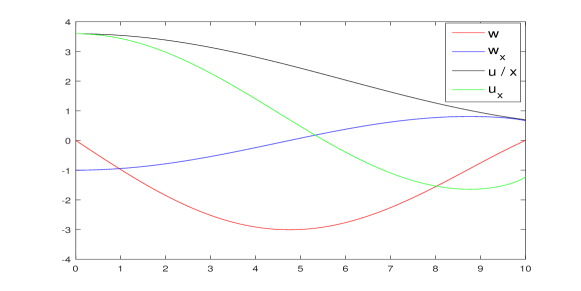
Figure 1. Approximate self-similar profile

All the numerical computations and quantitative verifications are performed by MATLAB (version 2019a) in the double-precision floating-point operation. The MATLAB codes can be found via the link [3]. To make sure that our computer-assisted proof is rigorous, we adopt the standard method of interval arithmetic (see [42, 39]). In particular, we use the MATLAB toolbox INTLAB (version 11 [43]) for the interval computations. Every single real number $p$ in MatLab is represented by an interval $[p_{l},p_{r}]$ that contains $p$, where $p_{l},p_{r}$ are precise floating-point numbers of 16 digits. Every computation of real number summation, multiplication or division is performed using the interval arithmetic, and the outcome is hence represented by the resulting interval $[P_{l},P_{r}]$ that strictly contains $P$. We then obtain a rigorous upper bound on $|P|$ by rounding up $\max\{|P_{l}|,|P_{r}|\}$ to 2 significant digits (or 4 when necessary). We remark that, when encountering a non-essential ill-conditioned computation, especially a division, we will replace it by an alternative well-conditioned one. For example, for some function $f(x)$ such that $f(0)=0,f_{x}(0)<+\infty$, the evaluation of $\frac{f(x)}{x}$ at $x=0$ will be replaced by the evaluation of $f_{x}(0)$.

4.1.1. Compact support of the approximate profile

The approximate profile $\bar{\omega}$ we obtain actually has compact support. Below we explain how we obtain a compactly supported approximate self-similar profile. First let us assume that $\omega$ is a solution of the steady state equation (or equivalently self-similar equation), i.e. taking $\omega_{t}=0$ in (4.1),

$$(c_{l}x+u)\omega_{x}=(c_{\omega}+u_{x})\omega,\quad u_{x}=H\omega.$$

Differentiating both sides and then evaluating the resulting equation at $x=0$, we obtain

$$(c_{l}+u_{x})\omega_{x}|_{x=0}=(c_{\omega}+u_{x})\omega_{x}|_{x=0},$$

which implies $c_{l}=c_{\omega}$, provided that $\omega_{x}(0)\neq 0$. Suppose that we have a finite time self-similar blowup. Then the scaling factor $c_{\omega}$ is negative. See the discussion in Section 3.1. It follows that $c_{l}=c_{\omega}<0$. This also holds true for the approximate profile: $\bar{c}_{l}=\bar{c}_{\omega}<0$. Moreover, we have that $\bar{u}>0$ for $x>0$ and grows sublinearly for large $x$. The difference between the signs of $\bar{c}_{l}x$ and $\bar{u}(x)$ and their different growth rates for large $|x|$ lead to the following change of sign in the approximate profile

$$\bar{c}_{l}x_{0}+\bar{u}(x_{0})=0,\quad\bar{c}_{l}x+\bar{u}(x)>0\textrm{ for }0\leq x<x_{0},\quad\bar{c}_{l}x+\bar{u}(x)<0\textrm{ for }x>x_{0},$$

for some $x_{0}>0$. We expect that a similar change of sign occurs in the dynamic variable $c_{l}x+u$ and the solution of (4.1) will form a shock. When we solve $\bar{\omega}$ numerically, we can fix the point where the sign of $c_{l}x+u$ changes by imposing (4.2). Moreover, the approximate profile satisfies that $\bar{c}_{\omega}+\bar{u}_{x}(x)$ is negative for $x>x_{0}$ (see Figure 1). For $x>x_{0}$, we expect that the dynamic variable $c_{\omega}+u_{x}(x)$ is also negative, which implies that $(c_{\omega}+u_{x}(x))\omega$ in (4.1) is a damping term. For $x>x_{0}$, due to the transport term $(c_{l}x+u)\omega_{x}$ with $c_{l}x+u(x)<0$ and the damping effect $(c_{\omega}+u_{x}(x))\omega$, the solution tends to have compact support. For this reason, in our computation, we have chosen the initial data with compact support and controlled the support of the solution by imposing (4.2). As a result, the approximate profile also has compact support.

4.1.2. Regularity of the approximate profile

In the domain $[-L,L]$, since $\bar{\omega}$ is obtained from the cubic spline interpolation, it has the regularity $C^{2,1}[-L,L]$. Moreover, since $\bar{\omega}(x)=0$ for $|x|\geq L$, $\bar{\omega}$ is a Lipschitz function on the real line. We remark that $\bar{\omega}$ is in $H^{1}(\mathbf{R})$ but not in $H^{2}(\mathbf{R})$ since $\bar{\omega}_{x}$ is discontinuous at $x=\pm L$, i.e. $\omega_{x}(\pm L)\neq 0$ (see Figure 1). Multiplying $(x^{2}-L^{2})$, we get a compactly supported and global Lipschitz function $(x^{2}-L^{2})\bar{\omega}_{x}$. Hence we can define the Hilbert transform of $((x^{2}-L^{2})\bar{\omega}_{x})_{x}$ which is in $L^{p}$ for any $1\leq p<+\infty$.

Applying (A.4) in Lemma A.2, we have

$$\bar{u}_{xx}=H\bar{\omega}_{x},\quad\bar{u}_{xxx}(x^{2}-L^{2})=H(\bar{\omega}_{xx}(x^{2}-L^{2})).$$

Using the regularity of $\bar{\omega}$, we have that $\bar{u}$ is at least $C^{3}$ in $(-L,L)$ and $\bar{u}_{xx}$ grows logarithmically near $x=\pm L$ since $\bar{\omega}_{x}$ is discontinuous at $x=\pm L$.

4.1.3. Regularity of the perturbation

We will choose odd initial perturbation $\omega_{0}$ such that $\omega_{0}+\bar{\omega}\in C_{c}^{\infty}$ and $\omega_{0,x}(0)=0$. Standard local well-posedness result shows that $\omega+\bar{\omega}$ remains smooth locally in time. Hence, the regularity of $\omega$ and $\bar{\omega}$ are the same before blowup. Since the odd symmetry of the solution $\omega+\bar{\omega}$ is preserved and $\bar{\omega}$ is odd, this implies that $\omega$ is odd. From this property and $\omega_{x}(0)=0$ (see (4.3)), $\omega$ is of order $O(x^{3})$ near $x=0$. On the other hand, we have $\omega(\pm L)=0$ since its support lies in $[-L,L]$. In the following derivation, the boundary terms when we perform integration by parts on $\omega$ terms will vanish, which can be justified by these vanishing conditions. We will use this property without explicitly mentioning it.

In [34], the De Gregorio model (1.3) with $a=1$ was solved numerically on $\mathbb{R}$ for $t\in[0,1]$. The author demonstrated the growth of the solution numerically and plotted the solutions at several times that have similar profiles, which share some similar structure with our $\bar{\omega}$.

4.2. Linear stability of the approximate self-similar profile

Linear stability analysis plays a crucial role in establishing the existence and stability of the self-similar profile. We will establish the linear stability of the approximate self-similar profile in this subsection.

Linearizing (4.1) around $\bar{\omega},\bar{u},\bar{c}_{l},\bar{c}_{\omega}$ yields

(4.4) $$\omega_{t}+(\bar{c}_{l}x+\bar{u})\omega_{x}=(\bar{c}_{\omega}+\bar{u}_{x})\omega+(u_{x}+c_{\omega})\bar{\omega}-(u+c_{l}x)\bar{\omega}_{x}+N(\omega)+F(\bar{\omega})\;,$$

where $\omega,u,c_{l},c_{\omega}$ are the perturbations of the approximate self-similar profile, $N$ and $F$ are the nonlinear terms and the residual error, respectively

(4.5) $$N(\omega)=(c_{\omega}+u_{x})\omega-(c_{l}x+u)\omega_{x},\quad F(\bar{\omega})=(\bar{c}_{\omega}+\bar{u}_{x})\bar{\omega}-(\bar{c}_{l}x+\bar{u})\bar{\omega}_{x}.$$

Main ideas in our linear stability analysis

Compared to (3.9), (4.4) does not contain a small parameter $a$ in the nonlocal term $(u+c_{l}x)\bar{\omega}_{x}$, which makes it substantially harder to establish linear stability. There are three key observations in our linear stability estimates. First of all, we observe that the $u_{x}\bar{\omega}$ term (vortex stretching) is harmless to the linear stability analysis as we have shown in Section 3. We construct the weight function carefully to fully exploit the cancellation between $u_{x}$ and $\omega$ (see Lemma A.3). Secondly, we observe that there is a competition between the advection term $u\omega_{x}$ and the vortex stretching term $u_{x}\omega$. We expect some cancellation between their perturbation $u\bar{\omega}_{x}$ and $u_{x}\bar{\omega}$. By exploiting this cancellation, we obtain a sharper estimate of $u/x$ by $\omega$, which improves the corresponding estimate using the Hardy inequality (A.8). Roughly speaking, for $x$ close to $0$, the term $u/x$ can be bounded by $\omega/5$ in some appropriate norm; similarly, for $x$ close to $L$, the term $(u(x)-u(L))/(x-L)$ can be bounded by $\omega/3$ in some appropriate norm. The small constants, $1/5$ and $1/3$, are essential for us to obtain sharp estimates on the non-local term $u$. If we had used a rough estimate with constant $1/5$ replacing by $1/2$, we would have failed to establish linear stability. Using the first two observations, the estimate of most interactions can be reduced to the estimate of some boundary terms. In order to obtain a sharp stability constant, we express these boundary terms as the projection of $\omega$ onto some functions and exploit the cancellation between different projections to obtain the desired linear stability estimate.

Due to the odd symmetry of $u,\omega$, we just need to focus on the positive real line. Denote

$$\langle f,g\rangle\triangleq\int_{0}^{L}fgdx,\quad||f||_{p}=||f||_{L^{p}[0,L]}$$

for any $1\leq p\leq\infty$. For most integrals we consider, it is the same as the integral from $0$ to $+\infty$ since the support of $\omega$ lies in $[-L,L]$. Define a singular weight function on $[0,L]$

(4.6) $$\varphi\triangleq\left(-\frac{1}{x^{3}}-\frac{e}{x}-\frac{f\cdot 2x}{L^{2}-x^{2}}\right)\cdot\left(\chi_{1}\left(\bar{\omega}-\frac{x\bar{\omega}_{x}}{5}\right)+\chi_{2}\left(\bar{\omega}-\frac{(x-L)\bar{\omega}_{x}}{3}\right)\right)^{-1},$$

where $\chi_{1},\chi_{2}\geq 0$ are cutoff functions such that $\chi_{1}+\chi_{2}=1$ and

$$\chi_{1}(x)=\begin{cases}1&x\in[0,4]\\ 0&x\in[6,10]\\ \end{cases},\quad\chi_{1}(x)=\frac{\exp\left(\frac{1}{x-4}+\frac{1}{x-6}\right)}{1+\exp\left(\frac{1}{x-4}+\frac{1}{x-6}\right)}\ \forall x\in[4,6].$$

Note that the denominator in (4.6) is negative in $(0,L)$ and that $\varphi>0$ is a singular weight and is of order $O(x^{-4})$ near $x=0$, $O((x-L)^{-2})$ near $x=L$.

Performing the weighted $L^{2}$ estimate on (4.4) yields

(4.7) $$\frac{1}{2}\frac{d}{dt}\langle\omega^{2},\varphi\rangle =\Big{\langle}-(\bar{c}_{l}x+\bar{u})\omega_{x}+(\bar{c}_{w}+\bar{u}_{x})\omega,\omega\varphi\Big{\rangle}+\Big{\langle}(u_{x}+c_{\omega}),\bar{\omega}\omega\varphi\rangle-\langle(c_{l}x+u),\bar{\omega}_{x}\omega\varphi\Big{\rangle}$$

$$+\langle N(\omega),\omega\varphi\rangle+\langle F(\bar{\omega}),\omega\varphi\rangle\triangleq D+I+N_{1}+F_{1}.$$

Note that the support of the perturbation lies in $[-L,L]$, the above integral is effectively from $0$ to $L$. For $D$, we use integration by parts to obtain

(4.8) $$D=\Big{\langle}\frac{1}{2\varphi}((\bar{c}_{l}x+\bar{u})\varphi)_{x}+(\bar{c}_{w}+\bar{u}_{x}),\omega^{2}\varphi\Big{\rangle}\triangleq\langle D(\bar{\omega}),\omega^{2}\varphi\rangle.$$

From (4.6), we know that $\varphi(x)=O(x^{-4})$ near $x=0$ and $\varphi(x)=O((x-L)^{-2})$ near $x=L$. Using these asymptotic properties of $\varphi$, one can obtain that

$$D(\bar{\omega})(0)=-(\bar{c}_{l}+\bar{u}_{x}(0))/2<0,\quad D(\bar{\omega})(L)=(\bar{c}_{l}+\bar{u}_{x}(L))/2<0.$$

We can verify rigorously that $D(\bar{\omega})(x)$ is negative on $[0,L)$ pointwisely. In particular, we treat $\langle D(\bar{\omega}),\omega^{2}\varphi\rangle$ as a damping term. See Section 2.1 for the discussions on the derivation of the damping term.

We estimate the interaction near $x=0$ and $x=L$ differently. First we split the $I$ term into two terms as follows:

(4.9) $$I=\langle(u_{x}+c_{\omega})\bar{\omega}-(c_{l}x+u)\bar{\omega}_{x},\omega\varphi\chi_{1}\rangle+\langle(u_{x}+c_{\omega})\bar{\omega}-(c_{l}x+u)\bar{\omega}_{x},\omega\varphi\chi_{2}\rangle\triangleq I_{1}+I_{2}.$$

We use different decompositions of $(u_{x}+c_{\omega})\bar{\omega}-(c_{l}x+u)\bar{\omega}_{x}$ for $x$ close to $0$ and to $L$. For $x$ close to $0$ (the $\chi_{1}$ part), we use $c_{\omega}=c_{l}$ to obtain

$$(u_{x}+c_{\omega})\bar{\omega}-(c_{l}x+u)\bar{\omega}_{x}=(u_{x}+c_{\omega})\left(\bar{\omega}-\frac{1}{5}\bar{\omega}_{x}x\right)+x\bar{\omega}_{x}\left(\frac{1}{5}(u_{x}+c_{\omega})-\frac{u+c_{l}x}{x}\right)$$

$$= (u_{x}+c_{\omega})\left(\bar{\omega}-\frac{1}{5}\bar{\omega}_{x}x\right)+x\bar{\omega}_{x}\left(\frac{1}{5}(u_{x}-u_{x}(0))-\frac{u-u_{x}(0)x}{x}-\frac{4}{5}(c_{\omega}+u_{x}(0))\right).$$

For $x$ close to $L$ (the $\chi_{2}$ part), using $c_{\omega}=c_{l}=-u(L)/L$ (4.2), we have

$$u+c_{l}x=u-u(L)+c_{l}(x-L).$$

Therefore, we obtain

$$(u_{x}+c_{\omega})\bar{\omega}-(c_{l}x+u)\bar{\omega}_{x}=(u_{x}+c_{\omega})\bar{\omega}-(x-L)\bar{\omega}_{x}\cdot\frac{u-u(L)+c_{l}(x-L)}{x-L}$$

$$= (u_{x}+c_{\omega})\left(\bar{\omega}-\frac{1}{3}\bar{\omega}_{x}(x-L)\right)+(x-L)\bar{\omega}_{x}\left(\frac{1}{3}(u_{x}+c_{\omega})-\frac{u-u(L)+c_{l}(x-L)}{x-L}\right)$$

$$= (u_{x}+c_{\omega})\left(\bar{\omega}-\frac{1}{3}\bar{\omega}_{x}(x-L)\right)+(x-L)\bar{\omega}_{x}\left(\frac{1}{3}(u_{x}-u_{x}(L))-\frac{u-u(L)-u_{x}(L)(x-L)}{x-L}\right)$$

$$-\frac{2}{3}(x-L)\bar{\omega}_{x}(c_{\omega}+u_{x}(L)).$$

Using (4.9) and the above decompositions near $x=0$, we get

(4.10) $$I_{1} =\Big{\langle}\left(\frac{1}{5}\frac{u_{x}-u_{x}(0)}{x^{2}}-\frac{u-u_{x}(0)x}{x^{3}}\right),x^{3}\bar{\omega}_{x}\omega\varphi\chi_{1}\Big{\rangle}+\Big{\langle}(c_{\omega}+u_{x}),\left(\bar{\omega}-\frac{1}{5}\bar{\omega}_{x}x\right)\omega\chi_{1}\varphi\Big{\rangle}$$

$$-\frac{4}{5}(c_{\omega}+u_{x}(0))\langle x\bar{\omega}_{x},\omega\chi_{1}\varphi\rangle\triangleq I_{11}+I_{12}+I_{13}.$$

Similarly, near $x=L$, we have

(4.11) $$I_{2} =\Big{\langle}\left(\frac{1}{3}\frac{u_{x}-u_{x}(L)}{x-L}-\frac{u-u(L)-u_{x}(L)(x-L)}{(x-L)^{2}}\right)(x-L)^{2}\bar{\omega}_{x}\omega\varphi\chi_{2}\Big{\rangle}$$

$$+\Big{\langle}(c_{\omega}+u_{x}),\left(\bar{\omega}-\frac{1}{3}\bar{\omega}_{x}(x-L)\right)\omega\varphi\chi_{2}\Big{\rangle}-\frac{2}{3}(c_{\omega}+u_{x}(L))\langle(x-L)\bar{\omega}_{x},\omega\varphi\chi_{2}\rangle$$

$$\triangleq I_{21}+I_{22}+I_{23}.$$

4.2.1. The first part: the interior interaction

To handle the first term on the right hand side of (4.10) and (4.11), i.e. $I_{11},I_{21}$, we use the Cauchy-Schwarz inequality to obtain

(4.12) $$I_{11} \leq\Big{|}\Big{|}\left(\frac{1}{5}\frac{u_{x}-u_{x}(0)}{x^{2}}-\frac{u-u_{x}(0)x}{x^{3}}\right)\Big{|}\Big{|}_{2}||x^{3}\bar{\omega}_{x}\omega\varphi\chi_{1}||_{2},$$

$$I_{21} \leq\Big{|}\Big{|}\frac{1}{3}\frac{u_{x}-u_{x}(L)}{x-L}-\frac{u-u(L)-u_{x}(L)(x-L)}{(x-L)^{2}}\Big{|}\Big{|}_{2}||(x-L)^{2}\bar{\omega}_{x}\omega\varphi\chi_{2}||_{2}.$$

Using integration by parts yields

(4.13) $$\Big{|}\Big{|}\left(\frac{1}{5}\frac{u_{x}-u_{x}(0)}{x^{2}}-\frac{u-u_{x}(0)x}{x^{3}}\right)\Big{|}\Big{|}^{2}_{2}$$

$$= \frac{1}{25}\Big{|}\Big{|}\frac{u_{x}-u_{x}(0)}{x^{2}}\Big{|}\Big{|}^{2}_{2}-\frac{2}{5}\int_{0}^{L}\frac{(u_{x}-u_{x}(0))\cdot(u-u_{x}(0)x)}{x^{5}}dx+\Big{|}\Big{|}\frac{u-u_{x}(0)x}{x^{3}}\Big{|}\Big{|}^{2}_{2}$$

$$= \frac{1}{25}\Big{|}\Big{|}\frac{u_{x}-u_{x}(0)}{x^{2}}\Big{|}\Big{|}^{2}_{2}-\frac{1}{5}\frac{(u-u_{x}(0)x)^{2}}{x^{5}}\Big{|}_{0}^{L}-\frac{1}{5}\cdot 5\int_{0}^{L}\frac{(u-u_{x}(0)x)^{2}}{x^{6}}dx+\Big{|}\Big{|}\frac{u-u_{x}(0)x}{x^{3}}\Big{|}\Big{|}^{2}_{2}$$

$$= \frac{1}{25}\Big{|}\Big{|}\frac{u_{x}-u_{x}(0)}{x^{2}}\Big{|}\Big{|}^{2}_{2}-\frac{1}{5L^{5}}(u(L)-u_{x}(0)L)^{2}=\frac{1}{25}\Big{|}\Big{|}\frac{u_{x}-u_{x}(0)}{x^{2}}\Big{|}\Big{|}^{2}_{2}-\frac{1}{5L^{3}}(c_{\omega}+u_{x}(0))^{2}$$

$$\leq \frac{1}{25}\Big{|}\Big{|}\frac{\omega}{x^{2}}\Big{|}\Big{|}^{2}_{2}-\frac{1}{5L^{3}}(c_{\omega}+u_{x}(0))^{2},$$

where we have used $c_{\omega}=c_{l}=-u(L)/L$ in the second to the last line. To obtain the last inequality, we have used estimate (A.8) with $p=4$, the facts that the integral in $||\cdot||_{2}$ is from $0$ to $L$ and that $\omega$ supports in $[-L,L]$. Denote $v\triangleq u-u(L)-u_{x}(L)(x-L).$ Obviously, we have

$$v(L)=v_{x}(L)=0,\ v(0)=-u(L)+u_{x}(L)L=L(c_{\omega}+u_{x}(L)).$$

Using the above formula and integration by parts, we obtain

(4.14) $$\Big{|}\Big{|}\frac{1}{3}\frac{u_{x}-u_{x}(L)}{x-L}-\frac{u-u(L)-u_{x}(L)(x-L)}{(x-L)^{2}}\Big{|}\Big{|}_{2}^{2}=\Big{|}\Big{|}\frac{1}{3}\frac{v_{x}}{x-L}-\frac{v}{(x-L)^{2}}\Big{|}\Big{|}_{2}^{2}$$

$$= \frac{1}{9}\Big{|}\Big{|}\frac{v_{x}}{x-L}\Big{|}\Big{|}_{2}^{2}-\frac{2}{3}\int_{0}^{L}\frac{vv_{x}}{(x-L)^{3}}dx+\Big{|}\Big{|}\frac{v}{(x-L)^{2}}\Big{|}\Big{|}_{2}^{2}$$

$$= \frac{1}{9}\Big{|}\Big{|}\frac{v_{x}}{x-L}\Big{|}\Big{|}_{2}^{2}-\frac{1}{3}\frac{v^{2}}{(x-L)^{3}}\Big{|}^{L}_{0}-\frac{1}{3}\cdot 3\int_{0}^{L}\frac{v^{2}}{(x-L)^{4}}dx+\Big{|}\Big{|}\frac{v}{(x-L)^{2}}\Big{|}\Big{|}_{2}^{2}$$

$$= \frac{1}{9}\Big{|}\Big{|}\frac{v_{x}}{x-L}\Big{|}\Big{|}_{2}^{2}+\frac{1}{3}\frac{v(0)^{2}}{(0-L)^{3}}=\frac{1}{9}\Big{|}\Big{|}\frac{u_{x}-u_{x}(L)}{x-L}\Big{|}\Big{|}_{2}^{2}-\frac{1}{3L}(c_{\omega}+u_{x}(L))^{2}.$$

Using a formula similar to (A.1) yields

$$(u_{x}-u_{x}(L))(x-L)^{-1}=H\left(\omega(x-L)^{-1}\right).$$

We further obtain the following by using the $L^{2}$ isometry of the Hilbert transform

(4.15) $$\int_{0}^{L}\frac{(u_{x}-u_{x}(L))^{2}}{(x-L)^{2}}dx =\int_{x\in R}\frac{\omega^{2}}{(x-L)^{2}}dx-\int_{x\notin[0,L]}\frac{(u_{x}-u_{x}(L))^{2}}{(x-L)^{2}}dx.$$

Note that the Cauchy-Schwarz inequality implies

$$\int_{x\notin[0,L]}\frac{(u_{x}-u_{x}(L))^{2}}{(x-L)^{2}}dx\geq\int_{-L}^{0}\frac{(u_{x}-u_{x}(L))^{2}}{(x-L)^{2}}dx$$

$$\geq \left(\int_{-L}^{0}(u_{x}-u_{x}(L))dx\right)^{2}\left(\int_{-L}^{0}(x-L)^{2}dx\right)^{-1}$$

$$= (u(0)-u(-L)-u_{x}(L)L)^{2}\left(\frac{7}{3}L^{3}\right)^{-1}=\frac{3}{7}\frac{(c_{\omega}+u_{x}(L))^{2}L^{2}}{L^{3}}=\frac{3}{7}\frac{(c_{\omega}+u_{x}(L))^{2}}{L}.$$

Combining (4.14), (4.15) and the above inequality, we get

(4.16) $$\Big{|}\Big{|}\frac{1}{3}\frac{u_{x}-u_{x}(L)}{x-L}-\frac{u-u(L)-u_{x}(L)(x-L)}{(x-L)^{2}}\Big{|}\Big{|}_{2}^{2}$$

$$= \frac{1}{9}\int_{x\in R}\frac{\omega^{2}}{(x-L)^{2}}dx-\frac{1}{9}\int_{x\notin[0,L]}\frac{(u_{x}-u_{x}(L))^{2}}{(x-L)^{2}}dx-\frac{1}{3L}(c_{\omega}+u_{x}(L))^{2}$$

$$\leq \frac{1}{9}\int_{x\in R}\frac{\omega^{2}}{(x-L)^{2}}dx-\left(\frac{1}{3L}+\frac{1}{21L}\right)(c_{\omega}+u_{x}(L))^{2}.$$

Combining (4.12) , (4.13) and (4.16) and using the elementary inequality $xy\leq\lambda x^{2}+\frac{1}{4\lambda}y^{2}$, we obtain the estimate for $I_{11},I_{21}$,

(4.17) $$I_{11}+I_{21} \leq 25a_{1}\Big{|}\Big{|}\left(\frac{1}{5}\frac{u_{x}-u_{x}(0)}{x^{2}}-\frac{u-u_{x}(0)x}{x^{3}}\right)\Big{|}\Big{|}^{2}_{2}+\frac{1}{100a_{1}}||x^{3}\bar{\omega}_{x}\omega\varphi\chi_{1}||^{2}_{2}$$

$$+9a_{2}\Big{|}\Big{|}\frac{1}{3}\frac{u_{x}-u_{x}(L)}{x-L}-\frac{u-u(L)-u_{x}(L)(x-L)}{(x-L)^{2}}\Big{|}\Big{|}^{2}_{2}+\frac{1}{36a_{2}}||(x-L)^{2}\bar{\omega}_{x}\omega\varphi\chi_{2}||^{2}_{2}$$

$$\leq a_{1}\Big{|}\Big{|}\frac{\omega}{x^{2}}\Big{|}\Big{|}^{2}_{2}+\frac{1}{100a_{1}}||x^{3}\bar{\omega}_{x}\omega\varphi\chi_{1}||^{2}_{2}+a_{2}\int_{x\in R}\frac{\omega^{2}}{(x-L)^{2}}dx$$

$$+\frac{1}{36a_{2}}||(x-L)^{2}\bar{\omega}_{x}\omega\varphi\chi_{2}||^{2}_{2}-a_{2}\left(\frac{3}{L}+\frac{3}{7L}\right)(c_{\omega}+u_{x}(L))^{2},$$

where $a_{1},a_{2}>0$ are some parameters to be chosen later.

4.2.2. The second part

Combining $I_{12},I_{22}$ in (4.10), (4.11) respectively, and using the definition of $\varphi$ (4.6), we obtain

(4.18) $$I_{12}+I_{22}=\Big{\langle}(c_{\omega}+u_{x}),\left\{\left(\bar{\omega}-\frac{1}{5}\bar{\omega}_{x}x\right)\chi_{1}+\left(\bar{\omega}-\frac{1}{3}\bar{\omega}_{x}(x-L)\right)\chi_{2}\right\}\omega\varphi\Big{\rangle}$$

$$= \Big{\langle}(c_{\omega}+u_{x})\omega,\left(-\frac{1}{x^{3}}-\frac{e}{x}-\frac{f\cdot 2x}{L^{2}-x^{2}}\right)\Big{\rangle}$$

$$= (c_{\omega}+u_{x}(0))\Big{\langle}\omega,-\frac{1}{x^{3}}-\frac{e}{x}\Big{\rangle}+\Big{\langle}(u_{x}-u_{x}(0))\omega,-\frac{1}{x^{3}}-\frac{e}{x}\Big{\rangle}+\Big{\langle}(c_{\omega}+u_{x})\omega,-\frac{f\cdot 2x}{L^{2}-x^{2}}\Big{\rangle},$$

where $e$ and $f$ are constants in the definition of $\varphi$ (4.6). Since $\omega\in C^{2,1}$ and $\omega(0)=\omega_{x}(0)=\omega_{xx}(0)=0$, we have $\omega\cdot x^{-3}\in L^{1}$ and the above integrals are well-defined. Using (A.5) and (A.6), we obtain

(4.19) $$\Big{\langle}\frac{(u_{x}-u_{x}(0))w}{x^{3}}\Big{\rangle} =\frac{1}{2}\int_{\mathbf{R}}\frac{(u_{x}-u_{x}(0))w}{x^{3}}dx=0,$$

$$\Big{\langle}\frac{(u_{x}-u_{x}(0))\omega}{x}\Big{\rangle} =\frac{1}{2}\int_{\mathbf{R}}\frac{(u_{x}-u_{x}(0))w}{x}dx=\frac{\pi}{4}u_{x}^{2}(0).$$

Note that $(c_{\omega}+u_{x})\omega$ is odd. The Tricomi identity Lemma A.1 implies

(4.20) $$\Big{\langle}(c_{\omega}+u_{x})\omega,-\frac{2x}{L^{2}-x^{2}}\Big{\rangle}=-\int_{\mathbf{R}^{+}}(c_{\omega}+u_{x})\omega\left(\frac{1}{L-x}-\frac{1}{L+x}\right)dx$$

$$= -\int_{\mathbf{R}}\frac{(c_{\omega}+u_{x})\omega}{L-x}dx=-\pi H((c_{\omega}+u_{x})\omega)(L)=-\pi c_{\omega}H\omega(L)-\pi H(u_{x}\omega)(L)$$

$$= -\pi c_{\omega}u_{x}(L)-\frac{\pi}{2}(u_{x}^{2}(L)-\omega^{2}(L))=-\pi c_{\omega}u_{x}(L)-\frac{\pi}{2}u_{x}^{2}(L).$$

Combining (4.18), (4.19) and (4.20), we obtain

(4.21) $$I_{12}+I_{22}=(c_{\omega}+u_{x}(0))\Big{\langle}\omega,\left(-\frac{1}{x^{3}}-\frac{e}{x}\right)\Big{\rangle}-\frac{\pi e}{4}u_{x}^{2}(0)-f\pi c_{\omega}u_{x}(L)-\frac{f\pi}{2}u_{x}^{2}(L).$$

4.2.3. The remaining part: the boundary interaction

Let $a_{3}\triangleq a_{2}(\frac{3}{L}+\frac{3}{7L})$. The negative term that appears in the last term of (4.17) can be written as

(4.22) $$-a_{2}(\frac{3}{L}+\frac{3}{7L})(c_{\omega}+u_{x}(L))^{2}=-a_{3}(c_{\omega}+u_{x}(L))^{2}.$$

Combining (4.22), (4.21), $I_{13},I_{23}$ in (4.10) and (4.11), we obtain

(4.23) $$I_{12}+I_{22}+I_{13}+I_{23}-a_{3}(c_{\omega}+u_{x}(L))^{2}$$

$$= (c_{\omega}+u_{x}(0))\Big{\langle}\omega,\left(-\frac{1}{x^{3}}-\frac{e}{x}\right)\Big{\rangle}-\frac{e\pi}{4}u_{x}^{2}(0)-f\pi c_{\omega}u_{x}(L)-\frac{f\pi}{2}u_{x}^{2}(L)$$

$$-\frac{4}{5}(c_{\omega}+u_{x}(0))\langle\omega,x\bar{\omega}_{x}\chi_{1}\varphi\rangle-\frac{2}{3}(c_{\omega}+u_{x}(L))\langle\omega,(x-L)\bar{\omega}_{x}\chi_{2}\varphi\rangle-a_{3}(c_{\omega}+u_{x}(L))^{2}$$

$$= u_{x}(0)\left(\Big{\langle}\omega,\left(-\frac{1}{x^{3}}-\frac{e}{x}\right)-\frac{4}{5}x\bar{\omega}_{x}\chi_{1}\varphi\Big{\rangle}-\frac{e\pi}{4}u_{x}(0)\right)$$

$$+c_{\omega}\left(\Big{\langle}\omega,\left(-\frac{1}{x^{3}}-\frac{e}{x}\right)-\frac{4}{5}x\bar{\omega}_{x}\chi_{1}\varphi-\frac{2}{3}(x-L)\bar{\omega}_{x}\chi_{2}\varphi\Big{\rangle}-f\pi u_{x}(L)-a_{3}c_{\omega}\right)$$

$$+u_{x}(L)\left(\Big{\langle}w,-\frac{2}{3}(x-L)\bar{\omega}_{x}\chi_{2}\varphi\Big{\rangle}-\frac{f\pi}{2}u_{x}(L)-2a_{3}c_{\omega}-a_{3}u_{x}(L)\right).$$

Note that

$$u_{x}(0) =-\frac{2}{\pi}\int_{0}^{L}\frac{\omega}{x}dx,\quad u_{x}(L)=\frac{1}{\pi}\int_{0}^{L}\frac{2x}{L^{2}-x^{2}}\omega dx,$$

$$c_{\omega} =-\frac{u(L)}{L}=\frac{1}{L\pi}\int_{0}^{L}\log\left(\frac{L+x}{L-x}\right)\omega(x)dx.$$

All the integrals in (4.23) and $c_{\omega},u_{x}(0),u_{x}(L)$ are the projection of $\omega$ onto some explicit functions. We use the cancellation of these functions to obtain a sharp estimate of the right hand side of (4.23). Denote

(4.24) $$g_{c_{\omega}} \triangleq\frac{1}{L\pi}\log\left(\frac{L+x}{L-x}\right),\quad g_{u_{x}(0)}\triangleq-\frac{2}{\pi x},\quad g_{u_{x}(L)}\triangleq\frac{2x}{\pi(L^{2}-x^{2})},$$

$$g_{1} \triangleq\left(-\frac{1}{x^{3}}-\frac{e}{x}\right)-\frac{4}{5}x\bar{\omega}_{x}\chi_{1}\varphi-\frac{e\pi}{4}g_{u_{x}(0)},$$

$$g_{2} \triangleq\left(-\frac{1}{x^{3}}-\frac{e}{x}\right)-\frac{4}{5}x\bar{\omega}_{x}\chi_{1}\varphi-\frac{2}{3}(x-L)\bar{\omega}_{x}\chi_{2}\varphi-f\pi g_{u_{x}(L)}-a_{3}g_{c_{\omega}},$$

$$g_{3} \triangleq-\frac{2}{3}(x-L)\bar{\omega}_{x}\chi_{2}\varphi-\left(\frac{f\pi}{2}+a_{3}\right)g_{u_{x}(L)}-2a_{3}g_{c_{\omega}}.$$

With these notations, we can rewrite (4.23) as follows

(4.25) $$u_{x}(0)\langle\omega,g_{1}\rangle+c_{\omega}\langle\omega,g_{2}\rangle+u_{x}(L)\langle\omega,g_{3}\rangle$$

$$= \langle\omega,g_{u_{x}(0)}\rangle\langle\omega,g_{1}\rangle+\langle\omega,g_{c_{\omega}}\rangle\langle\omega,g_{2}\rangle+\langle\omega,g_{u_{x}(L)}\rangle\langle\omega,g_{3}\rangle.$$

For some function $R\in C([0,L]),R>0$ to be chosen, we introduce

(4.26) $$y \triangleq(R\varphi)^{1/2}\omega,\quad f_{1}\triangleq(R\varphi)^{-1/2}g_{u_{x}(0)},\quad f_{2}\triangleq(R\varphi)^{-1/2}g_{1},\quad f_{3}\triangleq(R\varphi)^{-1/2}g_{c_{\omega}},$$

$$f_{4} \triangleq(R\varphi)^{-1/2}g_{2},\quad f_{5}\triangleq(R\varphi)^{-1/2}g_{u_{x}(L)},\quad f_{6}\triangleq(R\varphi)^{-1/2}g_{3}.$$

Our goal is to find the best constant of the following inequality for any $\omega\in L^{2}(\varphi)$

(4.27) $$\langle f_{1},y\rangle\langle f_{2},y\rangle+\langle f_{3},y\rangle\langle f_{4},y\rangle+\langle f_{5},y\rangle\langle f_{6},y\rangle \leq C_{opt}||y||_{2}^{2},$$

which is equivalent to

$$\langle\omega,g_{u_{x}(0)}\rangle\langle\omega,g_{1}\rangle+\langle\omega,g_{c_{\omega}}\rangle\langle\omega,g_{2}\rangle+\langle\omega,g_{u_{x}(L)}\rangle\langle\omega,g_{3}\rangle\leq C_{opt}\langle R,\omega^{2}\varphi\rangle,$$

so that we can estimate (4.25) by $\langle R,\omega^{2}\varphi\rangle$ with a sharp constant. From the definition of functions $g,f$, we have that $g_{3}\in\mathrm{span}(g_{c_{\omega}},g_{u_{x}(0)},g_{u_{x}(L)},g_{1},g_{2})$ and

(4.28) $$f_{6}\in\mathrm{span}(f_{1},f_{2},..,f_{5})\triangleq V,\quad\mathrm{dim}V=5.$$

Without loss of generality, we assume $y\in V$ since $||Py||_{2}\leq||y||_{2}$ and $\langle y,f_{i}\rangle=\langle Py,f_{i}\rangle$, where $P$ is the orthogonal projector onto $V$. Suppose that $\{e_{i}\}_{i=1}^{5}$ is an orthonormal basis (ONB) in $V$ with respect to the $L^{2}$ inner product on $[0,L]$. It can be obtained via the Gram-Schmidt procedure. Then we have $z=\sum_{i=1}^{5}\langle z,e_{i}\rangle e_{i}$ for any $z\in V$. We consider the linear map $T:V\to R^{5}$ defined by $(Tz)_{i}=\langle z,e_{i}\rangle,\ \forall z\ \in V$. It is obvious that $T$ is a linear isometry from $(V,\langle\cdot,\cdot\rangle_{L^{2}})$ to $R^{5}$ with the Euclidean inner product, i.e. $||Tz||_{l^{2}}=||z||_{L^{2}}$. Denote $v=Ty,v_{i}=Tf_{i}\in R^{5}$ . Using the linear isometry, i.e. $\langle f_{i},y\rangle=v^{T}v_{i}$ and $||y||^{2}_{2}=v^{T}v$, we can reduce (4.27) to

$$\sum_{1\leq i\leq 3}(v^{T}v_{2i-1})(v_{2i}^{T}v)=v^{T}(\sum_{1\leq i\leq 3}v_{2i-1}v_{2i}^{T})v\leq C_{opt}v^{T}v.$$

Denote $M\triangleq\sum_{1\leq i\leq 3}v_{2i-1}v_{2i}^{T}\in R^{5\times 5}$. Then the above inequality becomes $v^{T}Mv\leq C_{opt}v^{T}v$. Using the fact that $v^{T}Mv=v^{T}M^{T}v$, we can symmetrize it to obtain

$$v^{T}\frac{M+M^{T}}{2}v\leq C_{opt}v^{T}v.$$

Since $(M^{T}+M)/2$ is symmetric, the optimal constant $C_{opt}$ is the maximal eigenvalue of $(M+M^{T})/2$, i.e.

(4.29) $$C_{opt}=\lambda_{\max}\left(\frac{M+M^{T}}{2}\right)=\lambda_{\max}(\frac{1}{2}\sum_{1\leq i\leq 3}(v_{2i-1}v_{2i}^{T}+v_{2i}v_{2i-1}^{T})).$$

We remark that maximal eigenvalue $\lambda_{\max}$ is independent of the choice of the ONB of $V$. For other ONB, the resulting $\lambda_{\max}$ will be $\lambda_{\max}(Q(M+M^{T})Q^{T}/2)$ for some orthonormal matrix $Q\in R^{5\times 5}$, which is the same as (4.29). Using (4.23), (4.25), (4.27) and (4.29), we have proved

(4.30) $$I_{12}+I_{22}+I_{13}+I_{23}-a_{3}(c_{\omega}+u_{x}(L))^{2}\leq\lambda_{\max}(\frac{1}{2}\sum_{1\leq i\leq 3}(v_{2i-1}v_{2i}^{T}+v_{2i}v_{2i-1}^{T}))\langle R,\omega^{2}\varphi\rangle,$$

where $v_{i}\in R^{5}$ is the coefficient of $f_{i}$ (see (4.26)) expanded under an ONB $\{e_{i}\}_{i=1}^{5}$ of $V=\mathrm{span}(f_{1},f_{2},..,f_{5})$, i.e. the $j$-th component of $v_{i}$ satisfies $v_{ij}=\langle f_{i},e_{j}\rangle$. We will choose $R$ so that $\lambda_{\max}<1$ and then the left hand side can be controlled by $\langle R,\omega^{2}\varphi\rangle$.

4.2.4. Summary of the estimates

In summary, we collect all the estimates of $I_{ij},i=1,2,j=1,2,3$, (4.10), (4.11), (4.17) and (4.30) to conclude

(4.31) $$\langle(u_{x}+c_{\omega})\bar{\omega}-(c_{l}x+u),\bar{\omega}_{x},\omega\varphi\rangle=I=I_{1}+I_{2}=\sum_{i=1,2,j=1,2,3}I_{ij}$$

$$\leq a_{1}\Big{|}\Big{|}\frac{\omega}{x^{2}}\Big{|}\Big{|}^{2}_{2}+\frac{1}{100a_{1}}||x^{3}\bar{\omega}_{x}\omega\varphi\chi_{1}||^{2}_{2}+a_{2}\int_{x\in R}\frac{\omega^{2}}{(x-L)^{2}}dx$$

$$+ \frac{1}{36a_{2}}||(x-L)^{2}\bar{\omega}_{x}\omega\varphi\chi_{2}||^{2}_{2}+\lambda_{\max}(\frac{1}{2}\sum_{1\leq i\leq 3}(v_{2i-1}v_{2i}^{T}+v_{2i}v_{2i-1}^{T}))\langle R,\omega^{2}\varphi\rangle$$

$$\triangleq \langle A(\bar{\omega}),\omega^{2}\varphi\rangle+\lambda_{\max}(\frac{1}{2}\sum_{1\leq i\leq 3}(v_{2i-1}v_{2i}^{T}+v_{2i}v_{2i-1}^{T}))\langle R,\omega^{2}\varphi\rangle,$$

where $A(\bar{\omega})$ is the sum of the four terms in the first inequality and is given by

$$A(\bar{\omega})=\left(\frac{a_{1}}{x^{4}}+\frac{a_{2}}{(x-L)^{2}}+\frac{a_{2}}{(x+L)^{2}}\right)\varphi^{-1}+\frac{(x^{3}\bar{\omega}_{x}\chi_{1})^{2}\varphi}{100a_{1}}+\frac{((x-L)^{2}\bar{\omega}_{x}\chi_{2})^{2}\varphi}{36a_{2}}.$$

Optimizing the parameters

To optimize the estimate, we choose

(4.32) $$e =0.005,\ f=0.004,\ a_{1}=\frac{1}{6},\ a_{2}=1.4f=0.0056,\ a_{3}=a_{2}(3+\frac{3}{7})/L=0.00192.$$

After specifying these parameters, the coefficient of the damping term $D(\bar{\omega})$ (see (4.7)) and the coefficient of the estimate of the interior interaction $A(\bar{\omega})$ are completely determined. Then we choose

(4.33) $$R(\bar{\omega})=-D(\bar{\omega})-A(\bar{\omega})-0.3$$

in (4.26). The numerical values of $D(\bar{\omega})$, $A(\bar{\omega})$ and $R(\bar{\omega})$ on the grid points are plotted in the first subfigure in Figure 2. We can verify rigorously (see the discussion below) that $R(\bar{\omega})=-D(\bar{\omega})-A(\bar{\omega})-0.3>0$. In particular, the coefficient of the damping term satisfies $D(\bar{\omega})<-0.3-A(\bar{\omega})$ and is negative pointwisely. The corresponding $f_{i}$ in (4.27) are determined. The optimal constant in (4.30) can be computed :

(4.34) $$C_{opt}=\lambda_{\max}(\frac{1}{2}\sum_{1\leq i\leq 3}(v_{2i-1}v_{2i}^{T}+v_{2i}v_{2i-1}^{T}))<1.$$

Combining $\langle D(\bar{\omega}),\omega^{2}\varphi\rangle$ in (4.7), (4.31) and (4.34), we obtain the linear estimate

(4.35) $$\frac{1}{2}\frac{d}{dt}\langle\omega^{2},\varphi\rangle=\langle D(\bar{\omega}),\omega^{2}\varphi\rangle+I+N_{1}+F_{1}$$

$$\leq \langle D(\bar{\omega}),\omega^{2}\varphi\rangle+\langle A(\bar{\omega}),\omega^{2}\varphi\rangle+\langle R(\bar{\omega}),\omega^{2}\varphi\rangle+N_{1}+F_{1}=-0.3\langle\omega^{2},\varphi\rangle+N_{1}+F_{1}.$$

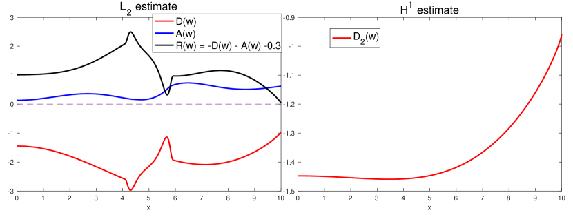
Figure 2. Left: Coefficients of the damping term $D(\bar{\omega})$ in the $L^{2}$ estimate, the estimate of the interior interaction $A(\bar{\omega})$ and the remaining terms $R(\bar{\omega})$. Right: Coefficient of the damping term $D_{2}(\bar{\omega})$ in the $H^{1}$ estimate.

For those who are not interested in the rigorous verification of the numerical values, they can skip the following discussion and jump to Section 4.4 for the weighted $H^{1}$ estimate.

4.3. Rigorous verification of the numerical values

We will use the following strategy to verify $R(\bar{\omega})>0$ (4.33), $C_{opt}<1$ (4.34) and $D_{2}(\bar{\omega})<-0.95$ (4.40) to be discussed later. These quantities appear in the weighted Sobolev estimates and are determined by the profile.

(a) Obtaining an explicit approximate self-similar profile. As described in section 4.1, our approximate self-similar profile $\bar{\omega}$ is expressed in terms of a piece-wise cubic polynomial over the grid points $x_{i}=\frac{iL}{n},i=0,\cdots,n$. The function values, $\bar{\omega}(x_{i}),\bar{\omega}_{x}(x_{i})$, which are used to construct the cubic Hermite spline, are computed accurately up to double-precision, and will be represented in the computations using the interval arithmetic with exact floating-point bounding intervals. All the following computer-assisted estimates are based on the rigorous interval arithmetic.

(b) Accurate point values of $\bar{u},\bar{u}_{x},\bar{u}_{xx}$. We have described how to compute the value of $\bar{u}_{x}(x)$ (or $\bar{u}(x),\bar{u}_{xx}(x)$) from certain integrals involving $\bar{\omega}$ on $[-L,L]$ in paragraph (3) in Section 4.1. For any $x\in[0,L]$, the integral contribution to $\bar{u}_{x}(x)$ from mesh intervals within $m=8$ mesh points distance from $x$ is computed exactly using analytic integration. In the outer domain that is $8h$ distance away from $x$, the integrand $\bar{\omega}(y)/(x-y)$ is not singular and we use a composite $8$-point Legendre-Gauss quadrature. There are two types of errors in this computation. The first type of error is the round-off error in the computation. The second type of error is due to the composite Gaussian quadrature that we use to approximate the integral in the outer domain. Notice that in each interval $[ih,(i+1)h]$ away from $x$, $\bar{\omega}$ is a cubic polynomial and the integrand $\bar{\omega}(y)/(x-y)$ is smooth. We can estimate high order derivatives of the integrand rigorously in these intervals. With the estimates of the derivatives, we can further establish error estimates of the Gaussian quadrature. In particular, we prove the following error estimates of the composite Gaussian quadrature in the computation of $\bar{u}_{x},\bar{u},\bar{u}_{xx}$ in the Supplementary material [4, Section 7]

$$Error_{GQ}(u_{x})<2\cdot 10^{-17},\quad Error_{GQ}(u)<2\cdot 10^{-19},\quad Error_{GQ}(u_{xx})<5\cdot 10^{-18}.$$

These two types of errors will be taken into account in the interval representations of $\bar{u}_{x}$. That is, each $\bar{u}_{x}(x)$ will be represented by $[\lfloor\bar{u}_{x}(x)-\epsilon\rfloor_{f},\lceil\bar{u}_{x}(x)+\epsilon\rceil_{f}]$ in any computation using the interval arithmetic, where $\lfloor\cdot\rfloor_{f}$ and $\lceil\cdot\rceil_{f}$ stand for the rounding down and rounding up to the nearest floating-point value, respectively. We remark that we will need the values of $\bar{u}_{x}(x)$ at finitely many points only. The same arguments apply to $\bar{u}(x)$ and $\bar{u}_{xx}(x)$ as well.

(c) Rigorous estimates of integrals. In many of our discussions, we need to rigorously estimate the integral of some function $g(x)$ on $[0,L]$. In particular, we want to obtain $c_{1},c_{2}$ such that $c_{1}\leq\int_{0}^{L}g(x)dx\leq c_{2}$. A straightforward way to do so is by constructing two sequences of values $g^{up}=\{g^{up}_{i}\}_{i=1}^{n},g^{low}=\{g^{low}_{i}\}_{i=1}^{n}$ such that

$$g^{up}_{i}\geq\max_{x\in[x_{i-1},x_{i}]}g(x)\quad\text{and}\quad g^{low}_{i}\leq\min_{x\in[x_{i-1},x_{i}]}g(x).$$

Then we can bound

$$h\cdot\sum_{i=1}^{n}g^{low}_{i}\leq\int_{0}^{L}g(x)dx\leq h\cdot\sum_{i=1}^{n}g^{up}_{i}.$$

In most cases, we will construct $g^{up}$ and $g^{low}$ from the grid point values of $g$ and an estimate of its first derivative. Let $g^{\max}=\{g^{\max}_{i}\}_{i=1}^{N}$ denote the sequence such that $g^{\max}_{i}=\max\{|g^{up}_{i}|,|g^{low}_{i}|\}$. Then if we already have $g_{x}^{\max}$, we can construct $g^{up}$ and $g^{low}$ as

$$g^{up}_{i}=g(x_{i})+h\cdot(g_{x}^{\max})_{i}\quad\text{and}\quad g^{low}_{i}=g(x_{i})-h\cdot(g_{x}^{\max})_{i}.$$

We can use this method to construct the piecewise upper bounds and lower bounds for many functions we need. For example, our approximate steady state $\bar{\omega}$ is constructed to be piecewise cubic polynomial using the standard cubic spline interpolation. Since $\bar{\omega}_{xxx}$ is piecewise constant, we have $\bar{\omega}_{xxx}^{up}$ and $\bar{\omega}_{xxx}^{low}$ for free from the grid point values of $\bar{\omega}$. Then we can construct $\bar{\omega}_{xx}^{up/low},\bar{\omega}_{x}^{up/low}$ and $\bar{\omega}^{up/low}$ recursively.

Note that for some explicit functions, we can construct the associated sequences of their piecewise upper bounds and lower bounds more explicitly. For example, for a monotone function $g$, $g^{up}$ and $g^{low}$ are just the grid point values.

Moreover, we can construct the piecewise upper bounds and lower bounds for more complicated functions. For instance, if we have $f_{a}^{up/low}$ and $f_{b}^{up/low}$ for two functions, then we can construct $g^{up/low}$ for $g=f_{a}f_{b}$ using standard interval arithmetic. In this way, we can estimate the integral of all the functions we need in our computer-aided arguments.

Sometimes we need to handle the ratio between two functions, which may introduce a removable singularity. For example, in the construction of $D(\bar{\omega})^{up}$ and $D(\bar{\omega})^{low}$ for $D(\bar{\omega})$ in (4.8), it involves $\frac{x\varphi_{x}}{\varphi},\frac{\bar{u}\varphi_{x}}{\varphi}$ and $\varphi$ is a singular weight of order $x^{-4}$ near $x=0$. Directly applying interval arithmetic to the ratio near a removable singularity can lead to large errors. We hence need to treat this issue carefully. For example, let us explain how to reasonably construct $g^{up/low}$ for a $g(x)=f(x)/x$ such that $f(x)$ has continuous first derivatives and $f(0)=0$. Suppose that we already have $f^{up/low}$ and $f_{x}^{up/low}$. Then for some small number $\varepsilon>0$, we let

$$g^{up}_{i}=\max\left\{\frac{f^{up}_{i}}{x_{i-1}},\frac{f^{low}_{i}}{x_{i-1}},\frac{f^{up}_{i}}{x_{i}},\frac{f^{low}_{i}}{x_{i}}\right\}\quad\text{for each index $i$ such that $x_{i-1}\geq\varepsilon$}.$$

Otherwise, for $x\in[0,\varepsilon)$, we have

$$g(x)=\frac{f(x)}{x}=f_{x}(\xi(x))\quad\text{for some $\xi(x)\in[0,x)\subset[0,\varepsilon)$}.$$

Then we choose $g^{up}_{i}=\max_{x\in[0,\varepsilon]}f_{x}^{up}$ for every index $i$ such that $x_{i}\leq\varepsilon$. The parameter $\varepsilon$ needs to be chosen carefully. On the one hand, $\varepsilon$ should be small enough so that the bound $f_{x}(\xi(x))\leq\max_{\tilde{x}\in[L-\varepsilon,L]}|f_{x}(\tilde{x})|$ is almost tight for $x\in[L-\varepsilon,L]$. On the other, the ratio $\varepsilon/h$ must be large enough so that $f^{up}_{i}/x_{i-1},f^{low}_{i}/x_{i-1},f^{up}_{i}/x_{i}$ and $f^{low}_{i}/x_{i}$ are close to each other for $x_{i-1}\geq\varepsilon$. Other kinds of removable singularities can be handled in a similar way.

See more detailed discussions in the Supplementary Material [4, Section 1.3].

(d) Estimates of some (weighted) norms of $\bar{\omega},\bar{u}$. Once we have used the preceding method to obtain $\bar{\omega}_{xxx}^{up/low},\bar{\omega}_{xx}^{up/low},\bar{\omega}_{x}^{up/low}$ and $\bar{\omega}^{up/low}$ from the grid point values of $\bar{\omega}$, we can further estimate some (weighted) norms of $\bar{\omega}$, e.g. $||\bar{\omega}_{x}||_{L^{\infty}},||\bar{\omega}_{xx}||_{L^{\infty}}$, rigorously. Moreover, from the discussion of the regularity of $\bar{u},\bar{\omega}$ in Section (4.1.2), the needed norms of $\bar{u}$, e.g. $||\bar{u}_{x}||_{\infty},||\bar{u}_{xx}||_{L^{2}}$, can be bounded by some norms of $\bar{\omega}$. See more detailed discussions in the Supplementary Material [4, Section 1.3].

(e) Rigorous and accurate estimates of certain integrals. Our rigorous estimate for integrals in the preceding part (c) is only first order accurate. Yet this method is not accurate enough if the target integral is supposed to be a very small number. When we need to obtain a more accurate estimate of the integral of some function $P$, we use the composite Trapezoidal rule

$$\int_{ah}^{bh}P(x)dx=\sum_{a\leq i<b}(P(x_{i})+P(x_{i+1}))h/2+\mathrm{error}(P).$$

The composite Trapezoidal rule uses the values of $P$ on the grid points only, which can be obtained up to the round off error. The numerical integral error, $\mathrm{error}(P)$, can be bounded by the $L^{1}$ norm of its second order derivative, i.e. $C||P^{\prime\prime}||_{L^{1}}h^{2}$ for some absolute constant $C$. We use this approach to obtain integral estimates of some functions involving the residual $F(\bar{\omega})$. For each function $P$ that we integrate, we prove in the Supplementary Material [4, Section 3] that $||P^{\prime\prime}||_{L^{1}}$ can be bounded by some (weighted) norms of $\bar{u},\bar{\omega}$, e.g. $||\bar{\omega}||_{L^{\infty}}$, $||\bar{u}_{x}||_{L^{\infty}}$ and $||\frac{\bar{\omega}_{xx}}{x}||_{L^{2}}$. Since these norms can be estimated by the method discussed previously, we can establish rigorous error bound for the integral.

(f) Rigorous estimates of $C_{opt}$. Denote by $M_{s}$ the matrix in (4.29)

$$M_{s}\triangleq\frac{1}{2}\sum_{i=1}^{3}(v_{2i-1}v_{2i}^{T}+v_{2i}v_{2i-1}^{T})=\frac{1}{2}V_{1}V_{2}^{T},$$

where $V_{1}\triangleq[v_{1},v_{2},v_{3},v_{4},v_{5},v_{6}]\in\mathbb{R}^{6\times 6}$ and $V_{2}\triangleq[v_{2},v_{1},v_{4},v_{3},v_{6},v_{5}]\in\mathbb{R}^{6\times 6}$, and $\{v_{i}\}_{i=1}^{6}$ are defined as in Section 4.2.3. Note that $M_{s}$ is symmetric, but not necessarily positive semidefinite. The optimal constant $C_{opt}$ is then the maximal eigenvalue of $M_{s}$. To rigorously estimate $C_{opt}$, we first bound it by the Schatten $p$-norm of $M_{s}$:

(4.36) $$C_{opt}\leq\|M_{s}\|_{p}\triangleq\mathrm{Tr}[|M_{s}|^{p}]^{1/p}\quad\text{for all $p\geq 1$}.$$

Here $|M_{s}|=\sqrt{M_{s}^{T}M_{s}}=\sqrt{M_{s}^{2}}$. In particular, if $p$ is an even number, we have $|M_{s}|^{p}=M_{s}^{p}$. Therefore,

$$\mathrm{Tr}[|M_{s}|^{p}]=2^{-p}\cdot\mathrm{Tr}[(V_{1}V_{2}^{T})^{p}]=2^{-p}\cdot\mathrm{Tr}[(V_{2}^{T}V_{1})^{p}]\triangleq 2^{-p}\cdot\mathrm{Tr}[X^{p}]$$

where $X=V_{2}^{T}V_{1}$. Note that each entry of $X$ is the inner product between some $v_{i}$ and $v_{j}$, $i,j=1,\dots,6$. Recall from (4.28) and its following paragraph that $v_{i}=Tf_{i},i=1,2,..,6$ and that $T:V\to R^{5}$ is a linear isometry. We have

$$\langle f_{i},f_{j}\rangle=\langle Tf_{i},Tf_{j}\rangle=v_{i}^{T}v_{j}.$$

Therefore, to compute the entries of $X$, we only need to compute the pairwise inner products between $f_{1},\dots,f_{6}$ (we do not need to compute the coordinate vectors $v_{i}$ explicitly). This is done by interval arithmetic based on the discussion in the preceding part (c). Therefore each entry $X_{ij}$ of $X$ is represented by a pair of numbers that we can bound from above and below. Once we have the estimate of $X$, we can compute an upper bound of $\mathrm{Tr}[X^{p}]$ stably and rigorously by interval arithmetic, which then gives a bound on $C_{opt}$ via (4.36). In particular, we choose $p=4$ in our computation, and we can rigorously verify that $C_{opt}<1$.

4.4. Weighted $H^{1}$ estimate

We choose

(4.37) $$\psi=-\frac{1}{\bar{\omega}}\left(\frac{1}{x}-\frac{x}{L^{2}}\right),\quad x\in[0,L],$$

as the weight for the weighted $H^{1}$ estimate. Note that the weight $\psi$ is nonnegative for $0\leq x\leq L$, and is of order $x^{-2}$ near $x=0$ and $O(1)$ near $x=L$. We can perform the weighted $H^{1}$ estimate as follows

(4.38) $$\frac{1}{2}\frac{d}{dt}\langle\omega_{x}^{2},\psi\rangle =\langle-((\bar{c}_{l}x+\bar{u})\omega_{x})_{x}+((\bar{c}_{\omega}+\bar{u}_{x})\omega)_{x},\omega_{x}\psi\rangle+\langle((u_{x}+c_{\omega})\bar{\omega})_{x},\omega_{x}\psi\rangle$$

$$-\langle((u+c_{l}x)\bar{\omega}_{x})_{x},\omega_{x}\psi\rangle+\langle N(\omega)_{x},\omega_{x}\psi\rangle+\langle F(\bar{\omega})_{x},\omega_{x}\psi\rangle$$

$$\triangleq I+II+III+N_{2}+F_{2}.$$

For $I$, we use $\bar{c}_{l}=\bar{c}_{\omega}$ and integration by parts to get

(4.39) $$I =\Big{\langle}-(\bar{c}_{l}x+\bar{u})\omega_{xx}+\bar{u}_{xx}\omega,\omega_{x}\psi\Big{\rangle}$$

$$=\Big{\langle}\frac{1}{2\psi}((\bar{c}_{l}x+\bar{u})\psi)_{x},\omega_{x}^{2}\psi\Big{\rangle}+\langle\bar{u}_{xx}\omega,\omega_{x}\psi\rangle\triangleq\langle D_{2}(\bar{\omega}),\omega_{x}^{2}\psi\rangle+\langle\bar{u}_{xx}\omega,\omega_{x}\psi\rangle.$$

The first term in $I$ is a damping term. We plot the numerical values of $D_{2}(\bar{\omega})$ on the grid points in Figure 2. We can verify rigorously that it is bounded from above by $-0.95$. Thus we have

(4.40) $$I=\langle D_{2}(\bar{\omega}),\omega_{x}^{2}\psi\rangle+\langle\bar{u}_{xx}\omega,\omega_{x}\psi\rangle\leq-0.95\langle\omega_{x}^{2},\psi\rangle+\langle\bar{u}_{xx}\omega,\omega_{x}\psi\rangle\triangleq-0.95\langle\omega_{x}^{2},\psi\rangle+I_{2},$$

where $I_{2}=\langle\bar{u}_{xx}\omega,\omega_{x}\psi\rangle$. For $II,III$, we note that

$$II+III =\langle u_{xx}\bar{\omega}+(u_{x}+c_{\omega})\bar{\omega}_{x}-(u_{x}+c_{l})\bar{\omega}_{x}-(c_{l}x+u)\bar{\omega}_{xx},\omega_{x}\psi\rangle$$

$$=\langle u_{xx}\bar{\omega},\omega_{x}\psi\rangle-\langle(c_{l}x+u)\bar{\omega}_{xx},\omega_{x}\psi\rangle\triangleq II_{1}+II_{2}.$$

Using the definition of $\psi$, we get

$$II_{1}=\langle u_{xx}\bar{\omega},\omega_{x}\psi\rangle=\Big{\langle}u_{xx}\omega_{x},-\frac{1}{x}+\frac{x}{L^{2}}\Big{\rangle}.$$

Since $\omega_{x}(0)=0$ by the normalization condition and $u_{xx}(0)=0$ by the odd symmetry, we can use the same cancellation as we did in (3.25) to get

$$\Big{\langle}u_{xx}\omega_{x},-\frac{1}{x}\Big{\rangle}=0,\quad\langle u_{xx}\omega_{x},x\rangle=0.$$

Therefore $II_{1}$ vanishes and we get

(4.41) $$II+III=II_{2}=-\langle(c_{l}x+u)\bar{\omega}_{xx},\omega_{x}\psi\rangle,$$

which is a cross term. In fact, after performing integration by parts, it becomes interaction among some lower order terms, i.e. of the order lower than $\omega_{x}$ (e.g. $u,u_{x},\omega$).

Remark 4.1.

So far, we have established all the delicate estimates of the linearized operator that exploit cancellations of various nonlocal terms. We have obtained the linear stability at the $L^{2}$ level and the linear stability estimates for the terms of the same order as $\omega_{x}$, e.g. $u_{xx}$, in the weighted $H^{1}$ estimates after performing integration by parts. The remaining estimates do not require specific structure of the equation. Suppose that we have a sequence of approximate steady states $\omega_{h_{i}}$ with $h_{i}$ converging to $0$ that enjoy similar estimates and have approximation error $\langle F(\omega_{h_{i}})^{2},\varphi\rangle+\langle F(\omega_{h_{i}})_{x}^{2},\psi\rangle$ of order $h_{i}^{\beta}$ for some constant $\beta>0$ independent of $h_{i}$, where $F(\omega_{h_{i}})$ is defined similarly as that in (4.5). Then we can apply the above stability analysis to the profile $\omega_{h}$ and the argument in Sections 3.2,3.3 to finish the remaining steps of the proof by choosing a sufficiently small $h=h_{n}$. Here $h$ plays a role similar to the small parameter $a$ in these sections. An important observation is that $h_{n}$ and the required approximation error to close the whole argument can be estimated effectively. Once we have determined $h_{n}$, we can construct the approximate steady state $\omega_{h_{n}}$ numerically and verify whether $\omega_{h_{n}}$ enjoys similar estimates and has the desired approximation error a posteriori.

In the following discussion, we first give some rough bounds and show that the remaining terms can be bounded by the weighted $L^{2}$ or $H^{1}$ norm of $\omega$ with constants depending continuously on $\bar{\omega}$. This property implies that similar bounds will also hold true if we replace the approximate steady state $\bar{\omega}$ by another profile $\hat{\omega}$, if $\bar{\omega}-\hat{\omega}$ is sufficiently small in some energy norm. We will provide other steps in the computer-assisted part of the paper later in this section.

The remaining linear terms in the weighted $H^{1}$ estimate are $I_{2}=\langle\bar{u}_{xx}\omega,\omega_{x}\psi\rangle$ in (4.40) and $II_{2}$ in (4.41). Denote $\rho=x^{-2}+(x-L)^{-2}$. Note that $u+c_{l}x|_{x=0,L}=0,c_{\omega}=c_{l}$. Applying integration by parts to the integral $||u_{x}+c_{l}-\frac{1}{2}(u+c_{l}x)/x||_{2}^{2},||u_{x}+c_{l}-\frac{1}{2}(u+c_{l}x)/(x-L)||_{2}^{2}$ and using an argument similar to those in (4.13), (4.14), we get

$$||(u+c_{l}x)\rho^{1/2}||_{2}^{2}=\int_{0}^{L}(u+c_{l}x)^{2}(\frac{1}{x^{2}}+\frac{1}{(x-L)^{2}})dx\leq 8\int_{0}^{L}(u_{x}+c_{l})^{2}dx.$$

Using the $L^{2}$ isometry of the Hilbert transform, the identity $\int_{0}^{L}u_{x}dx=u(L)=-L\cdot c_{l}$ and expanding the square, we further obtain

$$||(u+c_{l}x)\rho^{1/2}||_{2}^{2}\leq 8||\omega||_{2}^{2}+8(2c_{l}\cdot u(L)+Lc_{l}^{2})\leq 8||\omega||_{2}^{2}\leq 8||\varphi^{-1}||_{L^{\infty}}\langle\omega^{2},\varphi\rangle.$$

Applying the Cauchy-Schwarz inequality, we can estimate $I_{2},II_{2}$ as follows

$$|I_{2}| =|\langle\bar{u}_{xx}\omega,\omega_{x}\psi\rangle|\leq||\bar{u}_{xx}\psi^{1/2}\varphi^{-1/2}||_{L^{\infty}[0,L]}\langle\omega^{2},\varphi\rangle^{1/2}\langle\omega_{x}^{2},\psi\rangle^{1/2},$$

$$|II_{2}| =|\langle(c_{l}x+u)\bar{\omega}_{xx},\omega_{x}\psi|\rangle\leq||\rho^{-1/2}\bar{\omega}_{xx}\psi^{1/2}||_{L^{\infty}[0,L]}\langle(c_{l}x+u)^{2},\rho\rangle^{1/2}\langle\omega_{x}^{2},\psi\rangle^{1/2}.$$

Hence, combining the above estimates, we yield

(4.42) $$|I_{2}|+|II_{2}|\leq C_{1}(\bar{\omega})\langle\omega^{2},\varphi\rangle^{1/2}\langle\omega_{x}^{2},\psi\rangle^{1/2},\\$$

where

(4.43) $$C_{1}(\bar{\omega}) \triangleq||\bar{u}_{xx}\psi^{1/2}\varphi^{-1/2}||_{L^{\infty}[0,L]}+\sqrt{8}||\rho^{-1/2}\bar{\omega}_{xx}\psi^{1/2}||_{L^{\infty}[0,L]}||\varphi^{-1}||^{1/2}_{L^{\infty}}$$

and $\rho=x^{-2}+(x-L)^{-2}$. From the definitions of $\varphi,\psi$ (4.6), (4.37), the quantities appeared in $C_{1}(\bar{\omega})$ satisfy that

$$\varphi^{-1}=O((x^{-4}+(x-L)^{-2})^{-1}),\quad|\bar{u}_{xx}\psi^{1/2}\varphi^{-1/2}|=O(|\bar{u}_{xx}(x^{-1}+(L-x)^{-1})^{-1}|),$$

$$|(x^{-2}+(x-L)^{-2})^{-1/2}\bar{\omega}_{xx}\psi^{1/2}|=O(|(1+(x-L)^{-2})^{-1/2}\bar{\omega}_{xx}|).$$

In particular, these quantities are bounded for any $x\in[0,L]$ and thus $C_{1}(\bar{\omega})$ is finite.

Therefore, combining (4.38), (4.40), (4.41) and (4.42), we prove for any $\varepsilon>0$,

(4.44) $$\frac{1}{2}\frac{d}{dt}\langle\omega_{x}^{2},\psi\rangle\leq-0.95\langle\omega_{x}^{2},\psi\rangle+\varepsilon\langle\omega_{x}^{2},\psi\rangle+(4\varepsilon)^{-1}C_{1}(\bar{\omega})^{2}\langle\omega^{2},\varphi\rangle+N_{2}+F_{2},$$

From (4.35) and (4.44), we can choose $\varepsilon,\mu>0$ and construct the energy $E(t)^{2}=\langle\omega^{2},\varphi\rangle+\mu\langle\omega_{x}^{2},\psi\rangle$ such that

(4.45) $$\frac{d}{dt}E(t)^{2}\leq-C(\mu,\varepsilon)E(t)^{2}+N_{1}+F_{1}+\mu(N_{2}+F_{2}),$$

where $C(\mu,\varepsilon)>0$ depends on $\mu,\varepsilon$. For example, one can choose $\varepsilon=0.65,\;\mu=0.4\varepsilon C_{1}(\bar{\omega})^{-2}$ to obtain $C(\mu,\varepsilon)=0.2$. We have now completed the weighted $L^{2}$ and $H^{1}$ estimates at the linear level.

4.4.1. Nonlinear stability

Recall that $N,F$ are defined in (4.5), $N_{1},F_{1}$ in (4.7), and $N_{2},F_{2}$ in (4.38). Since $c_{l}=c_{\omega}$, a direct calculation yields $\partial_{x}N(\omega)=u_{xx}\omega-(c_{l}x+u)\omega_{xx}$.

Using integration by parts similar to that in (4.8) and (4.39), we obtain

$$N_{1}+\mu N_{2}=\Big{\langle}\frac{1}{2\varphi}(({c}_{l}x+u)\varphi)_{x}+(c_{\omega}+u_{x}),\omega^{2}\varphi\Big{\rangle}+\mu\Big{\langle}\frac{1}{2\psi}((c_{l}x+u)\psi)_{x},\omega_{x}^{2}\psi\Big{\rangle}+\mu\langle u_{xx}\omega,\omega_{x}\psi\rangle.$$

Recall $E(t)=(\langle\omega^{2},\varphi\rangle+\mu\langle\omega_{x}^{2},\psi\rangle)^{1/2}$. We can estimate $u_{x},\omega,u_{xx}$ as follows

$$||u_{x}||_{L^{\infty}} \leq 2||u_{x}||_{L^{2}(\mathbb{R}^{+})}^{1/2}||u_{xx}||_{L^{2}(\mathbb{R}^{+})}^{1/2}\leq 2||\omega||_{2}^{1/2}||\omega_{x}||_{2}^{1/2}$$

$$\leq 2\mu^{-1/4}||\varphi^{-1}||^{1/4}_{L^{\infty}}||\psi^{-1}||^{1/4}_{L^{\infty}}E(t),$$

$$||\omega||_{L^{\infty}} \leq||\omega_{x}||_{L^{1}}\leq\langle\omega_{x}^{2},\psi\rangle^{1/2}||\psi^{-1}||^{1/2}_{L^{1}[0,L]}\leq\mu^{-1/2}||\psi^{-1}||^{1/2}_{L^{1}[0,L]}E(t),$$

$$||u_{xx}x^{-1}||_{2} \leq||\omega_{x}x^{-1}||_{2}\leq\mu^{-1/2}||\psi^{-1/2}x^{-1}||_{L^{\infty}}E(t),$$

where we have used (A.3), $\omega_{x}(0)=0$ and the $L^{2}$ isometry of the Hilbert transform to obtain the last estimate. Recall $c_{l}=c_{\omega}=-u(L)/L$ (4.2). We have $c_{l}x+u|_{x=0,L}=0,|c_{l}|=|c_{\omega}|\leq||u_{x}||_{L^{\infty}}$ and

$$|c_{l}x+u| \leq\min(|x|,|L-x|)\cdot||c_{\omega}+u_{x}||_{L^{\infty}[0,L]}\leq 2\min(|x|,|L-x|)||u_{x}||_{\infty}.$$

For any $x\in[0,L]$, using the Leibniz rule, we derive

$$\Big{|}\frac{((c_{l}x+u)\varphi)_{x}}{\varphi}\Big{|}+\Big{|}\frac{((c_{l}x+u)\psi)_{x}}{\psi}\Big{|}\leq 2(2+\Big{|}\Big{|}(|x|\wedge(L-x))(\frac{|\varphi_{x}|}{\varphi}+\frac{|\psi_{x}|}{\psi})\Big{|}\Big{|}_{L^{\infty}})||u_{x}||_{L^{\infty}}\triangleq C_{2}(\bar{\omega})||u_{x}||_{L^{\infty}}.$$

Combining the above estimates, we prove

(4.46) $$N_{1}+\mu N_{2} \leq(C_{2}(\bar{\omega})+2)||u_{x}||_{L^{\infty}}(\langle\omega^{2},\varphi\rangle+\mu\langle\omega_{x}^{2},\psi\rangle)$$

$$+\mu||x\psi^{1/2}||_{L^{\infty}}||u_{xx}x^{-1}||_{2}||\omega||_{L^{\infty}}\langle\omega_{x}^{2},\psi\rangle^{1/2}\leq C_{3}(\bar{\omega},\mu)E(t)^{3},$$

where

$$C_{3}(\bar{\omega},\mu)=2\mu^{-1/4}(C_{2}(\bar{\omega})+2)||\varphi^{-1}||^{1/4}_{L^{\infty}}||\psi^{-1}||^{1/4}_{L^{\infty}}+\mu^{-1/2}||x\psi^{1/2}||_{L^{\infty}}||x^{-1}\psi^{-1/2}||_{L^{\infty}}||\psi^{-1}||^{1/2}_{L^{1}[0,L]}.$$

We remark that the above $L^{\infty}$ norms are taken over $[0,L]$. From the definition of $\varphi,\psi$, it is not difficult to verify that $C_{3}(\bar{\omega},\mu)<+\infty$.

To estimate the error term, we use the Cauchy-Schwarz inequality

(4.47) $$F_{1}+\mu F_{2} =\langle F(\bar{\omega}),\omega\varphi\rangle+\mu\langle F(\bar{\omega})_{x},\omega_{x}\psi\rangle$$

$$\leq(\langle F(\bar{\omega})^{2},\varphi\rangle+\mu\langle F(\bar{\omega})_{x}^{2},\psi\rangle)^{1/2}E(t)\triangleq\mathrm{error}(\bar{\omega})E(t),$$

Guideline for the remaining computer assisted steps

Recall the definition of $\varphi,\psi$ in (4.6) and (4.37). From the weighted $L^{2}$ and $H^{1}$ estimates, and the estimates of the nonlinear terms, we see that the coefficients and constants, e.g. $D(\bar{\omega})$ in (4.8), $C_{1}(\bar{\omega})$ in (4.43) and $C_{3}(\bar{\omega},\mu)$ in (4.46), depend continuously on $\bar{\omega}$. Hence, for two different approximate steady states $\omega_{h_{1}},\omega_{h_{2}}$ computed using different mesh $h_{2}<h_{1}$, if $\omega_{h_{1}}-\omega_{h_{2}}$ is small in some norm, e.g. some weighted $L^{2}$ or $H^{1}$ norm, we expect that all of these estimates hold true for these two profiles with very similar coefficients and constants. At the same time, the residual error of the profile computed using the finer mesh $\mathrm{error}(\omega_{h_{2}})$ can be much smaller than that of the coarse mesh $\mathrm{error}(\omega_{h_{1}})$. In particular, if the numerical solution $\omega_{h}$ exhibits convergence in a suitable norm as we refine the mesh size $h$, then we can obtain a sequence of approximate steady states that enjoy similar estimates with decreasing residual $\mathrm{error(\omega_{h})}$. See also the Remark 4.1. From our numerical computation, we did observe such convergence of $\omega_{h}$ computed using several meshes with decreasing mesh size $h$. Using the estimates that we have established, we can obtain nonlinear estimate for each profile $\bar{\omega}$ similar to (3.32)

$$\frac{1}{2}\frac{d}{dt}E^{2}(t)\leq-K_{1}(\bar{\omega})E^{2}(t)+K_{2}(\bar{\omega})E^{3}(t)+\mathrm{error}(\bar{\omega})E(t),$$

where $E(t)^{2}=\langle\omega^{2},\varphi\rangle+\mu(\bar{\omega})\langle\omega_{x}^{2},\psi\rangle$ and the positive constants $K_{1}(\bar{\omega}),K_{2}(\bar{\omega}),\mu(\bar{\omega})$ depend continuously on $\bar{\omega}$. From this inequality, we can estimate the size of $\mathrm{error}(\bar{\omega})$ that is required to close the bootstrap argument. A sufficient condition is that there exists $y>0$ such that $-K_{1}(\bar{\omega})y^{2}+K_{2}(\bar{\omega})y^{3}+\mathrm{error}(\bar{\omega})y<0$, which is equivalent to

(4.48) $$4\cdot\mathrm{error}(\bar{\omega})\cdot K_{2}(\bar{\omega})<K_{1}(\bar{\omega})^{2}.$$

Hence, we obtain a good estimate on $\mathrm{error}(\bar{\omega})$ that is required to close the whole estimate.

In practice, we first compute an approximate steady state $\bar{\omega}_{h}$ using a relatively coarse mesh, e.g. mesh size $h=L/1000$ or $L/2000$ (correspond to 1000 or 2000 grid points). Then we can perform all the weighted $L^{2}$, $H^{1}$ estimates and determine the weights $\varphi,\psi$, the decomposition in the estimates and all the parameters in (4.32) to obtain the linear stability, and perform the nonlinear estimates. After we obtain these estimates, we can determine a upper bound of $\mathrm{error}(\bar{\omega})$ using (4.48) and choose a finer mesh with mesh size $h_{2}$ to construct a profile $\bar{\omega}_{h_{2}}$ with a residual error less than this upper bound. After we extend all the corresponding estimates to the profile $\bar{\omega}_{h_{2}}$, we found that the corresponding constants and coefficients in the estimates are almost the same as those that we have obtained using $\bar{\omega}_{h}$ constructed by a coarser mesh. Therefore, we can perform analysis on $\bar{\omega}_{h_{2}}$ and close the whole argument.

In the Supplementary material [4, Sections 2,4], we will provide much sharper estimates of the cross terms (4.42), (4.44) and the nonlinear terms (4.46). These sharper estimates provide an estimate of the upper bound of $\mathrm{error}(\bar{\omega})$ in (4.48) that is not too small. This enables us to choose a modest mesh to construct an approximate profile with a residual error less than this upper bound. In particular, we choose $h=2.5\cdot 10^{-5}$ and the computational cost of $\bar{\omega}_{h}$ is affordable even for a personal laptop computer. The rigorous estimate for the residual error of this profile in the energy norm is established in the Supplementary material [4, Section 3]. More specifically, we can prove the following estimate, which improves the estimate given by (4.44) significantly.

Lemma 4.2.

The weighted $H^{1}$ estimate satisfies

$$\frac{1}{2}\frac{d}{dt}\langle\omega_{x}^{2},\psi\rangle=I+II_{2}+N_{2}+F_{2}\leq-0.25\langle\omega_{x}^{2},\psi\rangle+7.5\langle\omega^{2},\varphi\rangle+N_{2}+F_{2},$$

where $I,II_{2}$ combine the damping and the cross terms and are defined in (4.40), (4.41), respectively.

These refinements are not necessary if one can construct an approximate profile with a much smaller residual error using a more powerful computer with probably $10-100$ times more grid points. With these refined estimates and the rigorous estimate of the residual error of $\bar{\omega}_{h}$, we choose $\mu=0.02$ and bootstrap assumption $E(t)=\langle\omega^{2},\varphi\rangle+\mu\langle\omega_{x}^{2},\psi\rangle<5\cdot 10^{-4}$ to complete the final bootstrap argument. We refer the reader to the Supplementary material [4, Section 5] for the detailed estimates in the bootstrap argument.

The remaining steps are the same as those in the proof of Theorem 2. Recall the weights $\varphi$ (4.6) and $\psi$ (4.37) in the weighted $L^{2}$ and $H^{1}$ estimates and the regularity of the approximate profile $\bar{\omega}$ in Section 4.1.2. Note that $\varphi$ is of order $O(x^{-4})$ near $x=0$ and $O((x-L)^{-2})$ near $x=L$, and $\psi$ is of order $O(x^{-2})$ near $x=0$ and $O(1)$ near $x=L$. We can choose a small and odd initial perturbation $\omega$ supported in $[-L,L]$ with vanishing $\omega_{x}(0)=0$ such that $\omega$ restricted to $[0,L]$ satisfies $\omega\in L^{2}(\varphi),\omega_{x}\in L^{2}(\psi)$ and $\omega+\bar{\omega}\in C_{c}^{\infty}$. The bootstrap result implies that for all time $t>0$, the solution $\omega(t)+\bar{\omega}$, $c_{l}+\bar{c}_{l}=c_{\omega}(t)+\bar{c}_{\omega}$ remain close to $\bar{\omega},\bar{c}_{\omega}(\bar{c}_{\omega}<-0.69)$, respectively. Moreover, in the Supplementary Material [4, Section 6], we have established the following estimate

$$\frac{1}{2}\frac{d}{dt}\langle\omega_{t}^{2},\varphi\rangle\leq-0.15\langle\omega_{t}^{2},\varphi\rangle.$$

Using this estimate and a convergence argument similar to that in Section 3.3, we prove that the solution eventually converges to the self-similar profile $\omega_{\infty}$ with scaling factors $c_{l,\infty}=c_{\omega,\infty}<0$. Since $\gamma=-\frac{c_{l,\infty}}{c_{\omega,\infty}}=-1<0$, the asymptotically self-similar singularity is expanding. Thus we obtain an expanding and asymptotically self-similar blowup of the original De Gregorio model with scaling exponent $\gamma=-1$ in finite time.

5. Finite Time Blowup for $C^{\alpha}$ Initial Data

In [16], Elgindi and Jeong obtained the $C^{\alpha}$ self-similar solution $\omega_{\alpha}$ of the Constantin-Lax-Majda equation

$$c_{l}x\omega_{x}=(c_{\omega}+u_{x})\omega$$

for all $\alpha\in(0,1]$, which reads

(5.1) $$w_{\alpha} =-\frac{2\sin\left(\frac{\alpha\pi}{2}\right)\textrm{sgn}(x)|x|^{\alpha}}{1+2\cos\left(\frac{\alpha\pi}{2}\right)|x|^{\alpha}+|x|^{2\alpha}},\quad u_{\alpha,x}=\frac{2(1+\cos\left(\frac{\alpha\pi}{2}\right)|x|^{\alpha})}{1+2\cos\left(\frac{\alpha\pi}{2}\right)|x|^{\alpha}+|x|^{2\alpha}}\;,$$

$$c_{l} =\frac{1}{\alpha},\quad c_{\omega}=-1,$$

where $c_{l},c_{\omega}$ are the scaling parameters.

In this section, we will use the above solutions to construct approximate self-similar solutions analytically and use the same method of analysis presented in Section 3 to prove finite time asymptotically self-similar singularity for $C^{\alpha}$ initial data with small $\alpha$ on both the real line and on the circle. We will focus on solution of (1.3) with odd symmetry that is preserved during the evolution. In particular, we will construct odd approximate steady state and analyze the stability of odd perturbation around the approximate steady state.

5.1. Finite time blowup on $\mathbb{R}$ with $C_{c}^{\alpha}$ initial data

In this section, we prove Theorem 3. Throughout the proof, we impose $|a\alpha|<1$ and $\alpha<\frac{1}{4}$. We choose the following weights in the stability analysis

(5.2) $$\varphi_{\alpha}=-\frac{1}{\mathrm{sgn}(x)\omega_{\alpha}}\frac{1+2\cos\left(\frac{\alpha\pi}{2}\right)|x|^{\alpha}+|x|^{2\alpha}}{|x|^{1+2\alpha}},\quad\psi_{\alpha}=\frac{1}{\alpha^{2}}\varphi_{\alpha}x^{2}.$$

We choose these weights so that the estimates of $\langle\omega^{2},\varphi_{\alpha}\rangle$ and $\langle\omega_{x}^{2},\psi_{\alpha}\rangle$ are comparable in the energy estimates.

5.1.1. Normalization Conditions and Approximate Steady State

The self-similar equation of DG model with parameter $a$ reads

(5.3) $$(c_{l}x+au)\omega_{x}=(c_{\omega}+u_{x})\omega\;.$$

For any $a>0,\alpha\in(0,1)$, we construct $C^{\alpha}$ approximate self-similar profile of (5.3) below

(5.4) $$\omega_{\alpha},\quad u_{\alpha},\quad\bar{c}_{l,\alpha} =\frac{1}{\alpha}-au_{\alpha,x}(0)=\frac{1}{\alpha}-2a,\quad\bar{c}_{\omega}=-1.$$

The only difference between the above solution and the $C^{\alpha}$ self similar solutions of CLM (5.1) is the $c_{l}$ term. The above solution satisfies (5.3) up to an error

(5.5) $$F_{\alpha}(\omega_{\alpha})=-(\bar{c}_{l}x-\frac{1}{\alpha}x+au_{\alpha})\omega_{\alpha,x}=-a(u_{\alpha}-u_{\alpha,x}(0)x)\omega_{\alpha,x}.$$

Linearizing the dynamic rescaling equation (2.1) around the approximate self-similar profile in (5.4), we obtain the following equation for the perturbation $\omega,u,c_{l},c_{\omega}$

(5.6) $$\omega_{t}+(\bar{c}_{l,\alpha}x+au_{\alpha})\omega_{x}=(\bar{c}_{\omega}+u_{\alpha,x})\omega+(u_{x}+c_{\omega})\omega_{\alpha}-(au+c_{l}x)\omega_{\alpha,x}+N(\omega)+F_{\alpha}(\omega_{\alpha})\;,$$

where the error term $F_{\alpha}(\omega_{\alpha})$ is given in (5.5) and the nonlinear part is given by

$$N(\omega)=(c_{\omega}+u_{x})\omega-(c_{l}x+au)\omega_{x}.$$

We choose the following normalization conditions for $c_{l}(t),c_{\omega}(t)$

(5.7) $$c_{l}(t)=-au_{x}(t,0),\quad c_{\omega}(t)=-u_{x}(t,0).$$

Using (5.4) and $u_{\alpha,x}(0)=2$, we can rewrite the above conditions as

(5.8) $$c_{l}(t)+\bar{c}_{l}=\frac{1}{\alpha}-a(u_{x}(t,0)+u_{\alpha,x}(0)),\quad c_{\omega}+\bar{c}_{\omega}=1-(u_{x}(t,0)+u_{\alpha,x}(0)).$$

5.1.2. Estimate of the velocity, the self-similar solution and the error

We introduce the notation

(5.9) $$\tilde{u}\triangleq u-u_{x}(0)x,\quad\tilde{u}_{x}=u_{x}-u_{x}(0)\;,$$

and use the weighs defined in (5.2) to perform the $L^{2},H^{1}$ estimates.

We first state some useful properties of the $C^{\alpha}$ approximate self-similar solution that we will use in our stability analysis.

Lemma 5.1.

For $\alpha\in(0,1]$, we have the following estimates for the self-similar solutions defined in (5.1). (a) Uniform estimates on the damping effect

(5.10) $$\frac{1}{2\varphi_{\alpha}}\left(\frac{1}{\alpha}x\varphi_{\alpha}\right)_{x}+(\bar{c}_{\omega}+u_{\alpha,x})=-1/2\;,$$

$$\frac{1}{2\psi_{\alpha}}\left(\frac{1}{\alpha}x\psi_{\alpha}\right)_{x}+(\bar{c}_{\omega}+u_{\alpha,x})-\frac{1}{\alpha}=-1/2\;,$$

$$\frac{(u_{\alpha,xx}\psi_{\alpha})_{x}}{2\psi_{\alpha}}x^{2}=\frac{4\alpha^{2}|x|^{\alpha}(|x|^{\alpha}+\cos\left(\frac{\alpha\pi}{2}\right))}{(1+2\cos\left(\frac{\alpha\pi}{2}\right)|x|^{\alpha}+|x|^{2\alpha})^{2}}\geq 0\;.$$

(b) Vorticity and velocity estimates:

(5.11) $$\Big{|}\Big{|}\frac{xw_{\alpha,x}}{w_{\alpha}}\Big{|}\Big{|}_{\infty}\lesssim\alpha,\quad\Big{|}\Big{|}\frac{x^{2}w_{\alpha,xx}}{w_{\alpha}}\Big{|}\Big{|}_{\infty}\lesssim\alpha,\quad\Big{|}\Big{|}\frac{x^{2}\omega_{\alpha,xx}+x\omega_{\alpha,x}}{\omega_{\alpha}}\Big{|}\Big{|}_{\infty}\lesssim\alpha^{2}\;,$$

(5.12) $$\Big{|}\frac{u_{\alpha}}{x}-u_{\alpha,x}(0)\Big{|}\lesssim|x|^{\alpha}\wedge 1,\quad\Big{|}\frac{u_{\alpha}}{x}-u_{\alpha,x}\Big{|}\lesssim\alpha(|x|^{\alpha}\wedge 1)\;.$$

(c) Asymptotic estimates of $\varphi_{\alpha},\psi_{\alpha}$:

(5.13) $$\varphi_{\alpha}\asymp\frac{1}{\alpha}(|x|^{-1-3\alpha}+|x|^{-1+\alpha})\;,$$

$$\psi_{\alpha}=\frac{1}{\alpha^{2}}x^{2}\varphi_{\alpha}\asymp\frac{1}{\alpha^{3}}(|x|^{1-3\alpha}+|x|^{1+\alpha})\;,$$

$$\Big{|}\Big{|}\frac{x\psi_{\alpha,x}}{\psi_{\alpha}}-1\Big{|}\Big{|}_{\infty}\lesssim\alpha,\quad\Big{|}\Big{|}\frac{x\varphi_{\alpha,x}}{\varphi_{\alpha}}+1\Big{|}\Big{|}_{\infty}\lesssim\alpha\;,$$

where $A\asymp B$ means that $A\leq CB$ and $B\leq CA$ for some universal constant $C$.

(d) The smallness of the weighted $L^{2}$ and $H^{1}$ errors:

(5.14) $$\langle F_{\alpha}(\omega_{\alpha})^{2},\varphi_{\alpha}\rangle\lesssim a^{2}\alpha^{2},\quad\langle(F_{\alpha}(\omega_{\alpha}))_{x}^{2},\psi_{\alpha}\rangle\lesssim a^{2}\alpha^{2},$$

(5.15) $$\langle(|x|^{\alpha}\wedge 1)^{2}\omega^{2}_{\alpha,x},\psi_{\alpha}\rangle\lesssim 1.$$

These estimates are elementary and we defer the proof to the Appendix A.2.

Remark 5.2.

We will use (5.10) to derive the damping terms in the weighted $L^{2}$ and $H^{1}$ estimates. Using (5.11), we gain a small factor $\alpha$ from the derivatives of $\omega_{\alpha}$. This enables us to show that the perturbation term $u\omega_{\alpha,x}$ is small. Estimates (5.13) shows that $x\psi_{\alpha,x}/\psi_{\alpha},\ x\varphi_{\alpha,x}/\varphi_{\alpha}$ are close to $1$ and $-1$, respectively, which allows us to estimate $\varphi_{\alpha,x},\psi_{\alpha,x}$ effectively.

Lemma 5.3 ($L^{\infty}$ estimate).

(5.16) $$||u_{x}||_{\infty} \lesssim\langle\omega^{2},\varphi_{\alpha}\rangle^{1/4}\langle\omega_{x}^{2},\psi_{\alpha}\rangle^{1/4},$$

(5.17) $$\Big{|}\tilde{u}_{x}-\frac{\tilde{u}}{x}\Big{|} \lesssim\alpha\langle\omega_{x}^{2},\psi_{\alpha}\rangle^{1/2}|x^{\alpha}|\wedge 1\lesssim\alpha\langle\omega_{x}^{2},\psi_{\alpha}\rangle^{1/2},$$

(5.18) $$|\omega(x)| \lesssim\alpha\langle\omega_{x}^{2},\psi_{\alpha}\rangle^{1/2}|x^{\alpha}|\wedge 1,$$

where $\tilde{u}=u-u_{x}(0)x$.

We also defer the proof to the Appendix A.2. (5.17) shows that we can gain a small factor $\alpha$ from $\tilde{u}_{x}-\frac{\tilde{u}}{x}=u_{x}-u/x$.

We use a strategy similar to that in the proof of Theorem 2 to prove Theorem 3. The key step is establishing linear stability by taking advantage of the following:

(a) the stretching effect $\bar{c}_{l,\alpha}x\omega_{x}$ and the damping term $(\bar{c}_{\omega}+u_{x,\alpha})\omega$ ;

(b) the cancellation (A.11), (A.5) involving the vortex stretching term $u_{x}\omega_{\alpha}$;

(c) the smallness of the advection term $au\omega_{\alpha,x}$ (see (5.11)) by choosing $|a\alpha|$ to be sufficiently small .

To control the velocity $u$, we need to use Lemma A.4 in the Appendix, which states some nice properties of the Hilbert transform for a Hölder continuous function.

5.1.3. Linear Estimate

We first perform the weighted $L^{2}$ estimate with respect to (5.6). We proceed as follows

(5.19) $$\frac{1}{2}\frac{d}{dt}\langle\omega^{2},\varphi_{\alpha}\rangle =\langle-(\bar{c}_{l,\alpha}x+au_{\alpha})\omega_{x}+(\bar{c}_{\omega}+u_{\alpha,x})\omega,\omega\varphi_{\alpha}\rangle+\langle(u_{x}+c_{\omega})\omega_{\alpha},\omega\varphi_{\alpha}\rangle$$

$$-\langle(au+c_{l}x)\omega_{\alpha,x},\omega\varphi_{\alpha}\rangle+\langle N(\omega),\omega\varphi_{\alpha}\rangle+\langle F_{\alpha}(\omega_{\alpha}),\omega\varphi_{\alpha}\rangle$$

$$\triangleq I+II+III+N+F.$$

For $I$, we use integration by parts, (5.10) and $\bar{c}_{l,\alpha}=\frac{1}{\alpha}-au_{\alpha,x}(0)$ to get

(5.20) $$I =\Big{\langle}\frac{1}{2\varphi_{\alpha}}((\bar{c}_{l,\alpha}x+au_{\alpha})\varphi_{\alpha})_{x}+(\bar{c}_{\omega}+u_{\alpha,x}),\omega^{2}\varphi_{\alpha}\Big{\rangle}$$

$$=-\frac{1}{2}\langle\omega^{2},\varphi_{\alpha}\rangle+a\Big{\langle}\frac{1}{2\varphi_{\alpha}}((u_{\alpha}-u_{\alpha,x}(0)x)\varphi_{\alpha})_{x},\omega^{2}\varphi_{\alpha}\Big{\rangle}.$$

For the second term, we use (5.12) and (5.13) to yield

$$\Big{|}\frac{1}{2\varphi_{\alpha}}((u_{\alpha}-u_{\alpha,x}(0)x)\varphi_{\alpha})_{x}\Big{|}=\Big{|}\frac{1}{2}(u_{\alpha,x}-u_{\alpha,x}(0))+\frac{u_{\alpha}-u_{\alpha,x}(0)x}{x}\frac{x\varphi_{\alpha,x}}{2\varphi_{\alpha}}\Big{|}$$

$$= \Big{|}\frac{1}{2}(u_{\alpha,x}-\frac{u_{\alpha}}{x})+\frac{u_{\alpha}-u_{\alpha,x}(0)x}{x}\left(\frac{x\varphi_{\alpha,x}}{2\varphi_{\alpha}}+\frac{1}{2}\right)\Big{|}\lesssim\alpha+1\cdot\alpha\lesssim\alpha\;.$$

Combining (5.20) with the above estimate, we derive

(5.21) $$I\leq-\frac{1}{2}\langle\omega^{2},\varphi_{\alpha}\rangle+C|a|\alpha\langle\omega^{2},\varphi_{\alpha}\rangle=-\left(\frac{1}{2}-C|a|\alpha\right)\langle\omega^{2},\varphi_{\alpha}\rangle,$$

where $C>0$ is some universal constant.

Recall the definitions of $\varphi_{\alpha}$ in (5.2), $c_{l}=-au_{x}(0),c_{\omega}=-u_{x}(0)$ in (5.7) and $\tilde{u},\tilde{u}_{x}$ in (5.9). We have $c_{l}x+au=a\tilde{u},c_{\omega}+u_{x}=\tilde{u}_{x}$. For $II$, we use the cancellation (A.11) and (A.5) to get

(5.22) $$II =\langle\tilde{u}_{x}\omega_{\alpha},\omega\varphi_{\alpha}\rangle=-\Big{\langle}\tilde{u}_{x}\omega\cdot\mathrm{sgn}(x),|x|^{-1-2\alpha}+2\cos\left(\frac{\alpha\pi}{2}\right)||x|^{-1-\alpha}+|x|^{-1}\Big{\rangle}$$

$$\leq-\langle\tilde{u}_{x}\omega\cdot\mathrm{sgn}(x),|x|^{-1}\rangle=-\frac{\pi}{2}u_{x}^{2}(0)\leq 0.$$

For $III$, we have

$$|III| =|\langle(au+c_{l}x)\omega_{\alpha,x},\omega\varphi_{\alpha}\rangle|=\Big{|}a\Big{\langle}\frac{\tilde{u}}{x}\frac{\omega_{\alpha,x}x}{\omega_{\alpha}},\omega\frac{1+2\cos\left(\frac{\alpha\pi}{2}\right)|x|^{\alpha}+|x|^{2\alpha}}{|x|^{1+2\alpha}}\Big{\rangle}\Big{|}$$

$$\lesssim|a|\Big{\langle}\Big{|}\frac{\tilde{u}}{x}\Big{|}\Big{|}\frac{\omega_{\alpha,x}x}{\omega_{\alpha}}\Big{|},|\omega|(|x|^{-1-2\alpha}+|x|^{-1})\Big{\rangle}.$$

Using the estimate for $\omega_{\alpha}$ (5.11) and the Hardy inequality (A.12), we obtain

(5.23) $$|III| \lesssim|a|\alpha\Big{\langle}\Big{|}\frac{\tilde{u}}{x}\Big{|},|\omega|(|x|^{-1-2\alpha}+|x|^{-1})\rangle$$

$$\lesssim|a|\alpha\langle\tilde{u}^{2},|x|^{-3-3\alpha}\rangle^{1/2}\langle\omega^{2},|x|^{-1-\alpha}\rangle^{1/2}+|a|\alpha\langle\tilde{u}^{2},|x|^{-3-\alpha}\rangle^{1/2}\langle\omega^{2},|x|^{-1+\alpha}\rangle^{1/2}$$

$$\lesssim|a|\alpha\alpha^{-1}\langle\omega^{2},|x|^{-1-3\alpha}\rangle^{1/2}\langle\omega^{2},|x|^{-1-\alpha}\rangle^{1/2}+|a|\alpha\alpha^{-1}\langle\omega^{2},|x|^{-1-\alpha}\rangle^{1/2}\langle\omega^{2},|x|^{-1+\alpha}\rangle^{1/2}$$

$$\lesssim|a|\alpha\langle\omega^{2},\varphi_{\alpha}\rangle,$$

where we have used (5.13) to obtain the last inequality.

Plugging (5.21), (5.22) and (5.23) in (5.19), we arrive at

(5.24) $$\frac{1}{2}\frac{d}{dt}\langle\omega^{2},\varphi_{\alpha}\rangle\leq-\left(\frac{1}{2}-C|a|\alpha\right)\langle\omega^{2},\varphi_{\alpha}\rangle+\langle N(\omega),\omega\varphi_{\alpha}\rangle+\langle F_{\alpha}(\omega_{\alpha}),\omega\varphi_{\alpha}\rangle.$$

5.1.4. Weighted $H^{1}$ Estimate

Recall the definition of the weight $\psi_{\alpha}$ in (5.2). We now perform the weighted $H^{1}$ estimate with respect to (5.6)

(5.25) $$\frac{1}{2}\frac{d}{dt}\langle\omega_{x}^{2},\psi_{\alpha}\rangle =\langle-((\bar{c}_{l,\alpha}x+au_{\alpha})\omega_{x})_{x}+((\bar{c}_{\omega}+u_{\alpha,x})\omega)_{x},\ \omega_{x}\psi_{\alpha}\rangle$$

$$+\langle((u_{x}+c_{\omega})\omega_{\alpha})_{x},\ \omega_{x}\psi_{\alpha}\rangle-\langle((au+c_{l}x)\omega_{\alpha,x})_{x},\ \omega_{x}\psi_{\alpha}\rangle$$

$$+\langle N(\omega)_{x}.\omega_{x}\psi_{\alpha}\rangle+\langle F_{\alpha}(\omega_{\alpha})_{x},\ \omega_{x}\psi_{\alpha}\rangle\triangleq I+II+III+N_{2}+F_{2}.$$

For $I$, we again use integration by parts to obtain

$$I =\langle-(\bar{c}_{l,\alpha}x+au_{\alpha})\omega_{xx}-(\bar{c}_{l,\alpha}+au_{\alpha,x})\omega_{x}+(\bar{c}_{\omega}+u_{\alpha,x})\omega_{x},\omega_{x}\psi_{\alpha}\rangle+\langle u_{\alpha,xx}\omega,\omega_{x}\psi\rangle$$

$$=\Big{\langle}\frac{((\bar{c}_{l,\alpha}x+au_{\alpha})\psi_{\alpha})_{x}}{2\psi_{\alpha}}-(\bar{c}_{l,\alpha}+au_{\alpha,x})+(\bar{c}_{\omega}+u_{\alpha,x}),\omega_{x}^{2}\psi_{\alpha}\Big{\rangle}-\Big{\langle}\frac{(u_{\alpha,xx}\psi_{\alpha})_{x}}{2\psi_{\alpha}},\omega^{2}\psi\Big{\rangle}\triangleq I_{1}+I_{2}.$$

From (5.10), we get

$$I_{2}\leq 0.$$

Recall that $\bar{c}_{l,\alpha}=\frac{1}{\alpha}-au_{\alpha,x}$ and

$$\bar{c}_{l,\alpha}x+au_{\alpha,x}=\frac{1}{\alpha}+a(u_{\alpha}-u_{\alpha,x}x)=\frac{1}{\alpha}+a\tilde{u}_{\alpha},\quad\bar{c}_{l,\alpha}+au_{\alpha;x}=\frac{1}{\alpha}+\tilde{u}_{\alpha,x}.$$

We can use (5.10) to obtain

$$I_{1} =-\frac{1}{2}\langle\omega_{x}^{2},\psi_{\alpha}\rangle+a\Big{\langle}\frac{(\tilde{u}_{\alpha}\psi_{\alpha})_{x}}{2\psi_{\alpha}}-\tilde{u}_{\alpha,x},\omega_{x}^{2}\psi_{\alpha}\Big{\rangle}$$

$$=-\frac{1}{2}\langle\omega_{x}^{2},\psi_{\alpha}\rangle+a\Big{\langle}\frac{\tilde{u}_{\alpha}}{x}\frac{x\psi_{\alpha,x}}{2\psi_{\alpha}}-\frac{\tilde{u}_{\alpha,x}}{2},,\omega_{x}^{2}\psi_{\alpha}\Big{\rangle}.$$

Using (5.12) and (5.13), we get

$$\Big{|}\frac{\tilde{u}_{\alpha}}{x}\frac{x\psi_{\alpha,x}}{2\psi_{\alpha}}-\frac{\tilde{u}_{\alpha,x}}{2}\Big{|}\leq\Big{|}\frac{\tilde{u}_{\alpha}}{x}\Big{|}\cdot\Big{|}\frac{x\psi_{\alpha,x}}{2\psi_{\alpha}}-\frac{1}{2}\Big{|}+\frac{1}{2}\Big{|}\frac{\tilde{u}_{\alpha}}{x}-\tilde{u}_{\alpha,x}\Big{|}\lesssim||u_{\alpha,x}||_{\infty}\alpha+\alpha\lesssim\alpha.$$

It follows that

$$I_{1} \leq-\frac{1}{2}\langle\omega_{x}^{2},\psi_{\alpha}\rangle+C|a|\alpha\langle\omega_{x}^{2},\psi_{\alpha}\rangle=-\left(\frac{1}{2}-C|a|\alpha\right)\langle\omega_{x}^{2},\psi_{\alpha}\rangle,$$

(5.26) $$\Rightarrow I =I_{1}+I_{2}\leq I_{1}\leq-\left(\frac{1}{2}-C|a|\alpha\right)\langle\omega_{x}^{2},\psi_{\alpha}\rangle.$$

For $II$, we have

(5.27) $$II=-\langle u_{xx}\omega_{\alpha},\omega_{x}\psi_{\alpha}\rangle+\langle\tilde{u}_{x}\omega_{\alpha,x},\omega_{x}\psi_{\alpha}\rangle\triangleq II_{1}+II_{2}.$$

Note that

$$H(\omega_{x})=u_{xx},\ H(\omega_{x}x)(0)=0\Rightarrow H(\omega_{x}x)=u_{xx}x.$$

Moreover, we have that $\omega_{x}x$ is odd, $(xu_{xx})(0)=(x\omega_{x})(0)=0$. Applying the cancellation (A.11), (A.5) with $(u_{x},\omega)$ replaced by $(xu_{xx},x\omega_{x})$, we can estimate $II_{1}$ as follows

(5.28) $$II_{1} =-\Big{\langle}(xu_{xx})(x\omega_{x}),\frac{1}{\alpha^{2}}\frac{(1+2\cos\left(\frac{\alpha\pi}{2}\right)|x|^{\alpha}+|x|^{2\alpha})}{\mathrm{sgn}(x)|x|^{1+2\alpha}}\Big{\rangle}$$

$$\leq-\Big{\langle}(xu_{xx})(x\omega_{x}),\frac{1}{\mathrm{sgn}(x)\alpha^{2}|x|}\Big{\rangle}=-\frac{\pi}{2\alpha^{2}}(xu_{xx})(0)^{2}=0.$$

The remaining terms in the weighted $H^{1}$ estimate are $II_{2}$ in (5.27) and $III$ in (5.25), which can be decomposed as follows

$$III =-\langle((au+c_{l}x)\omega_{\alpha,x})_{x},\omega_{x}\psi_{\alpha}\rangle=-a\langle\tilde{u}_{x}\omega_{\alpha,x}+\tilde{u}\omega_{\alpha,xx},\omega_{x}\psi_{\alpha}\rangle$$

$$=-a\Big{\langle}(\tilde{u}_{x}-\frac{\tilde{u}}{x})\omega_{\alpha,x},\omega_{x}\psi_{\alpha}\Big{\rangle}-a\Big{\langle}\frac{\tilde{u}}{x}(\omega_{\alpha,x}+x\omega_{\alpha,xx}),\omega_{x}\psi_{\alpha}\Big{\rangle}\triangleq III_{1}+III_{2}.$$

We perform the estimate of $III_{1},III_{2}$ and the estimate of $II_{2}$ can be done similarly. Using the pointwise estimate (5.17) and the Cauchy Schwarz inequality, we can estimate $III_{1}$ as follows

(5.29) $$III_{1} \leq|a|\alpha\langle\omega_{x}^{2},\psi_{\alpha}\rangle^{1/2}\cdot\langle(|x|^{\alpha}\wedge 1)|\omega_{\alpha,x}|,|\omega_{x}|\psi_{\alpha}\rangle$$

$$\lesssim|a|\alpha\langle\omega_{x}^{2},\psi_{\alpha}\rangle\cdot\langle(|x|^{\alpha}\wedge 1)^{2}\omega^{2}_{\alpha,x},\psi_{\alpha}\rangle^{1/2}\lesssim|a|\alpha\langle\omega_{x}^{2},\psi_{\alpha}\rangle,$$

where we have used (5.15) to obtain the last inequality.

For $III_{2}$, we first use (5.11) to obtain

$$|III_{2}| =|a|\Big{|}\Big{\langle}\frac{\tilde{u}}{x}(\omega_{\alpha,x}+x\omega_{\alpha,xx}),\omega_{x}|x|^{1-2\alpha}\frac{(1+2\cos\left(\frac{\alpha\pi}{2}\right)|x|^{\alpha}+|x|^{2\alpha})}{\alpha^{2}\mathrm{sgn}(x)\omega_{\alpha}}\Big{\rangle}\Big{|}$$

$$=|a|\Big{|}\Big{\langle}\frac{\tilde{u}}{x^{2}}\frac{x(\omega_{\alpha,x}+x\omega_{\alpha,xx})}{\mathrm{sgn}(x)\omega_{\alpha}},\omega_{x}|x|^{1-2\alpha}\frac{(1+2\cos\left(\frac{\alpha\pi}{2}\right)|x|^{\alpha}+|x|^{2\alpha})}{\alpha^{2}}\Big{\rangle}\Big{|}$$

$$\lesssim|a|\Big{\langle}\Big{|}\frac{\tilde{u}}{x^{2}}\Big{|}\alpha^{2},|\omega_{x}|\ |x|^{1-2\alpha}\frac{(1+2\cos\left(\frac{\alpha\pi}{2}\right)|x|^{\alpha}+|x|^{2\alpha})}{\alpha^{2}}\Big{\rangle}$$

$$=|a|\Big{\langle}\Big{|}\frac{\tilde{u}}{x}\Big{|},|\omega_{x}|\left(1+2\cos\left(\frac{\alpha\pi}{2}\right)|x|^{-\alpha}+|x|^{-2\alpha}\right)\Big{\rangle}\lesssim|a|\Big{\langle}\Big{|}\frac{\tilde{u}}{x}\Big{|},|\omega_{x}|(1+|x|^{-2\alpha})\Big{\rangle}.$$

Then we use the Hardy inequality (A.12) to estimate $\tilde{u}$

$$|III_{2}| \lesssim|a|\Big{\langle}\Big{|}\frac{\tilde{u}}{x}\Big{|},|\omega_{x}|(1+|x|^{-2\alpha})\Big{\rangle}$$

$$\lesssim|a|\langle\tilde{u}^{2},|x|^{-3-3\alpha}\rangle^{1/2}\langle\omega_{x}^{2},|x|^{1-\alpha}\rangle^{1/2}+|a|\langle\tilde{u}^{2},|x|^{-3-\alpha}\rangle^{1/2}\langle\omega_{x}^{2},|x|^{1+\alpha}\rangle^{1/2}$$

$$\lesssim|a|\alpha^{-1}\langle\omega^{2},|x|^{-1-3\alpha}\rangle^{1/2}\langle\omega_{x}^{2},|x|^{1-\alpha}\rangle^{1/2}+|a|\alpha^{-1}\langle\omega^{2},|x|^{-1-\alpha}\rangle^{1/2}\langle\omega_{x}^{2},|x|^{1+\alpha}\rangle^{1/2}.$$

Using (5.13), we derive

(5.30) $$|III_{2}|\lesssim|a|\alpha^{-1}\alpha^{1/2}\langle\omega^{2},\varphi_{\alpha}\rangle^{1/2}\alpha^{3/2}\langle\omega_{x}^{2},\psi_{\alpha}\rangle^{1/2}=|a|\alpha\langle\omega^{2},\varphi_{\alpha}\rangle^{1/2}\langle\omega_{x}^{2},\psi_{\alpha}\rangle^{1/2}.$$

Similarly, for $II_{2}$, using the smallness $\Big{|}\Big{|}\frac{xw_{\alpha,x}}{w_{\alpha}}\Big{|}\Big{|}_{\infty}\lesssim\alpha$ in (5.11), the weighted estimate (A.9) and estimate of $\psi_{\alpha},\varphi_{\alpha}$ (5.13), one can obtain

(5.31) $$|II_{2}|\lesssim\langle\omega^{2},\varphi_{\alpha}\rangle^{1/2}\langle\omega_{x}^{2},\psi_{\alpha}\rangle^{1/2}.$$

Plugging (5.26), (5.27), (5.28), (5.29), (5.30) and (5.31) in (5.25), we obtain

(5.32) $$\frac{1}{2}\frac{d}{dt}\langle\omega_{x}^{2},\psi_{\alpha}\rangle \leq-\left(\frac{1}{2}-C|a|\alpha\right)\langle\omega_{x}^{2},\psi_{\alpha}\rangle+C\langle\omega^{2},\varphi_{\alpha}\rangle^{1/2}\langle\omega_{x}^{2},\psi_{\alpha}\rangle^{1/2}$$

$$+\langle N(\omega)_{x},\omega_{x}\psi_{\alpha}\rangle+\langle F_{\alpha}(\omega_{\alpha})_{x},\ \omega_{x}\psi_{\alpha}\rangle,$$

for some universal constant $C$, where we have used $|a\alpha|<1$.

In the following two subsections, we aim to control the nonlinear and error terms

$$\langle N(\omega),\omega\varphi_{\alpha}\rangle,\ \langle F_{\alpha}(\omega_{\alpha}),\omega\varphi_{\alpha}\rangle,\ \langle N(\omega)_{x},\omega_{x}\psi_{\alpha}\rangle,\langle F_{\alpha}(\omega_{\alpha})_{x},\ \omega_{x}\psi_{\alpha}\rangle\\$$

in (5.24) and (5.32).

5.1.5. Estimates of nonlinear terms

Recall from (5.7) and (5.9) that

$$c_{l}x+au=a(u-u_{x}(0)x)=a\tilde{u},\quad c_{\omega}+u_{x}=u_{x}-u_{x}(0)=\tilde{u}_{x}.$$

For the nonlinear terms in (5.24) and (5.32), we use integration by parts to obtain

$$\langle N(\omega),\omega\varphi_{\alpha}\rangle =\langle(c_{\omega}+u_{x})\omega-(c_{l}x+au)\omega_{x},\omega\varphi_{\alpha}\rangle=\Big{\langle}\tilde{u}_{x}+\frac{(a\tilde{u}\varphi_{\alpha})_{x}}{2\varphi_{\alpha}},\omega^{2}\varphi_{\alpha}\Big{\rangle}$$

$$=\langle\tilde{u}_{x},\omega^{2}\varphi_{\alpha}\rangle+\frac{a}{2}\Big{\langle}\left(\tilde{u}_{x}+\frac{\tilde{u}}{x}\frac{x\varphi_{\alpha,x}}{\varphi_{\alpha}}\right),\omega^{2}\varphi_{\alpha}\Big{\rangle}\triangleq I_{1}+I_{2},$$

$$\langle N(\omega)_{x},\omega_{x}\psi_{\alpha}\rangle =\langle((c_{\omega}+u_{x})\omega-(c_{l}x+au)\omega_{x})_{x},\omega_{x}\psi_{\alpha}\rangle$$

$$=\langle u_{xx}\omega+\tilde{u}_{x}\omega_{x},\omega_{x}\psi_{\alpha}\rangle-a\Big{\langle}\tilde{u}_{x}\omega_{x}+\tilde{u}\omega_{xx},\omega_{x}\psi_{\alpha}\Big{\rangle}$$

$$=\langle\tilde{u}_{x}\omega_{x},\omega_{x}\psi_{\alpha}\rangle+\langle u_{xx}\omega,\omega_{x}\psi_{\alpha}\rangle+a\Big{\langle}-\tilde{u}_{x}+\frac{(\tilde{u}\psi_{\alpha})_{x}}{2\psi_{\alpha}},\omega^{2}_{x}\psi_{\alpha}\Big{\rangle}\triangleq II_{1}+II_{2}+II_{3}.$$

For each term $I_{i},II_{j}$, we use Lemma 5.3 to control the $L^{\infty}$ norm of $\omega,\tilde{u}/x,\tilde{u}_{x}$ or $\tilde{u}_{x}-\tilde{u}/x$, and use $\langle\omega^{2},\varphi_{\alpha}\rangle$, $\langle\omega_{x}^{2},\psi_{\alpha}\rangle$ to control other terms. We present the estimate of $II_{3}$ that has a large coefficient $a$ and is more complicated. Other terms can be estimated similarly. For $II_{3}$, we notice that

$$-\tilde{u}_{x}+\frac{(\tilde{u}\psi_{\alpha})_{x}}{2\psi_{\alpha}} =-\frac{1}{2}\tilde{u}_{x}+\frac{1}{2}\frac{\tilde{u}}{x}\frac{\psi_{\alpha,x}x}{\psi_{\alpha}}=-\frac{1}{2}\left(\tilde{u}_{x}-\frac{\tilde{u}}{x}\right)+\frac{1}{2}\frac{\tilde{u}}{x}\left(\frac{\psi_{\alpha,x}x}{\psi_{\alpha}}-1\right).$$

Then we use the $L^{\infty}$ estimate (5.17) to control $\tilde{u}_{x}-\tilde{u}/x$, (5.16) to control $\tilde{u}/x=u/x-u_{x}(0)$ and (5.13) to estimate the terms involving $\psi_{\alpha}$. This gives

(5.33) $$II_{3}=\frac{a}{2}\Big{\langle}-\left(\tilde{u}_{x}-\frac{\tilde{u}}{x}\right)+\frac{\tilde{u}}{x}\left(\frac{\psi_{\alpha,x}x}{\psi_{\alpha}}-1\right),\omega_{x}^{2}\psi_{\alpha}\Big{\rangle}$$

$$\lesssim|a|\left(\Big{|}\Big{|}\tilde{u}_{x}-\frac{\tilde{u}}{x}\Big{|}\Big{|}_{L^{\infty}}+||u_{x}||_{\infty}\Big{|}\Big{|}\frac{\psi_{\alpha,x}x}{\psi_{\alpha}}-1\Big{|}\Big{|}_{L^{\infty}}\right)\langle\omega_{x}^{2},\psi_{\alpha}\rangle$$

$$\lesssim(|a|\alpha\langle\omega_{x}^{2},\psi_{\alpha}\rangle^{1/2}+|a|\alpha\langle\omega^{2},\varphi_{\alpha}\rangle^{1/4}\langle\omega_{x}^{2},\psi_{\alpha}\rangle^{1/4})\langle\omega_{x}^{2},\psi_{\alpha}\rangle\lesssim(\langle\omega^{2},\varphi_{\alpha}\rangle+\langle\omega_{x}^{2},\psi_{\alpha}\rangle)^{3/2},$$

where we have used $|a\alpha|<1$. Similarly, we have

(5.34) $$I_{1},I_{2},II_{1},II_{2}\lesssim(\langle\omega^{2},\varphi_{\alpha}\rangle+\langle\omega_{x}^{2},\psi_{\alpha}\rangle)^{3/2}.$$

Combining (5.33) and (5.34), we obtain the following estimates for the nonlinear terms

(5.35) $$\langle N(\omega),\omega\varphi_{\alpha}\rangle =I_{1}+I_{2}\lesssim(\langle\omega^{2},\varphi_{\alpha}\rangle+\langle\omega_{x}^{2},\psi_{\alpha}\rangle)^{3/2},$$

$$\langle N(\omega)_{x},\omega_{x}\psi_{\alpha}\rangle =II_{1}+II_{2}+II_{3}\lesssim(\langle\omega^{2},\varphi_{\alpha}\rangle+\langle\omega_{x}^{2},\psi_{\alpha}\rangle)^{3/2}.$$

5.1.6. Estimates of the error terms

Recall the error terms in the weighted $L^{2}$, $H^{1}$ estimates in (5.24) and (5.32) are given by

$$\langle F_{\alpha}(\omega_{\alpha}),\omega\varphi_{\alpha}\rangle,\quad\langle(F_{\alpha}(\omega_{\alpha}))_{x},\omega_{x}\psi_{\alpha}\rangle.$$

Using the Cauchy-Schwarz inequality and the error estimate (5.14), we obtain

(5.36) $$\langle F_{\alpha}(\omega_{\alpha}),\omega\varphi_{\alpha}\rangle \leq\langle F_{\alpha}(\omega_{\alpha})^{2},\varphi_{\alpha}\rangle^{1/2}\langle\omega^{2},\varphi_{\alpha}\rangle^{1/2}\lesssim|a|\alpha\langle\omega^{2},\varphi_{\alpha}\rangle^{1/2},$$

$$\langle(F_{\alpha}(\omega_{\alpha}))_{x},\omega_{x}\psi_{\alpha}\rangle \leq\langle(F_{\alpha}(\omega_{\alpha}))_{x}^{2},\psi_{\alpha}\rangle^{1/2}\langle\omega_{x}^{2},\psi_{\alpha}\rangle^{1/2}\lesssim|a|\alpha\langle\omega_{x}^{2},\psi_{\alpha}\rangle^{1/2}.$$

5.1.7. Nonlinear stability and convergence to self-similar solution

Now, we combine the weighted $L^{2}$, $H^{1}$ estimates (5.24), (5.32), the estimates of nonlinear terms (5.35) and error terms (5.36). Using these estimates and an argument similar to that in the analysis of nonlinear stability in Section 3.2 , we can choose an absolute constant $0<\mu$ such that the following energy

$$E^{2}(t)\triangleq\langle\omega^{2},\varphi_{\alpha}\rangle+\mu\langle\omega_{x}^{2},\psi_{\alpha}\rangle$$

satisfies the differential inequality

(5.37) $$\frac{1}{2}\frac{d}{dt}E^{2}(t)\leq-\left(\frac{3}{8}-C|a|\alpha\right)E^{2}(t)+C|a|\alpha E(t)+CE^{3}(t),$$

where $C>0$ is an absolute constant. From (5.13), we have

$$|u_{x}(0)|\lesssim\int|\omega_{x}(y)||\log(y)|dy\lesssim(\int\omega_{x}^{2}\psi_{\alpha})^{1/2}(\int\psi_{\alpha}^{-1}|\log y|^{2})^{1/2}$$

$$\lesssim E(t)\left(\alpha^{3}\int|\log y|^{2}(|y|^{1+\alpha}+|y|^{1-3\alpha})^{-1}dy\right)^{1/2}\lesssim E(t)(\alpha^{3}\alpha^{-1})^{1/2}\lesssim\alpha E(t).$$

The normalization condition (5.7) implies

(5.38) $$|c_{\omega}(t)|=|u_{x}(t,0)|\leq C_{3}\alpha E(t),\quad|c_{l}(t)|=|au_{x}(0)|\leq C_{3}|a|\alpha E(t),$$

for some absolute constant $C_{3}>0$.

Finally, we perform the bootstrap argument. We first choose $C_{2}=16C$, where $C$ is defined in (5.37), and then choose $C_{1}$ small such that

(5.39) $$C_{2}=16C,\quad CC_{1}+CC_{2}C_{1}+C_{3}C_{2}C_{1}+C_{1}<1/16.$$

Using the bootstrap argument and an argument similar to that in (3.32), we obtain that if

$$|a|\alpha<C_{1},\quad E(0)<C_{2}|a|\alpha,$$

then we must have $E(t)<C_{2}|a|\alpha<C_{2}C_{1}$. This is because the right hand side of (5.37) at $E(t)=C_{2}|a|\alpha$ is given by

$$E(t)^{2}\left(-\frac{3}{8}+C|a|\alpha+\frac{C|a|\alpha}{E(t)}+CE(t)\right)=E(t)^{2}\left(-\frac{3}{8}+(C+CC_{2})|a|\alpha+\frac{C}{C_{2}}\right)<-\frac{1}{4}E^{2}(t)<0.$$

Finally, we show that $c_{\omega}+\bar{c}_{\omega}<0$. The bootstrap results, (5.38) and (5.39) imply that

$$|c_{\omega}(t)|,|c_{l}(t)|<C_{3}E(t)<C_{3}C_{2}C_{1}<\frac{1}{16}\;.$$

It follows

(5.40) $$\bar{c}_{\omega}+c_{\omega}(t)=-1+c_{\omega}(t)<-\frac{1}{2},\quad\bar{c}_{l}+c_{l}(t)=\frac{1}{\alpha}-2a+c_{l}(t)>\frac{1}{2\alpha}-\frac{1}{16}\geq\frac{1}{4\alpha}.$$

As a result, we can choose small initial perturbation $\omega_{0}$ with $E(0)<C_{2}|a|\alpha$. Moreover, we choose $\omega_{0}$ in such a way that it modifies $\omega_{\alpha}$ at the far field to make the initial data $\bar{\omega}+\omega_{0}$ have compact support. The bootstrap result and $\bar{c}_{\omega}+c_{\omega}(\tau)<-1/2<0$ imply that the physical solution blows up in finite time.

5.1.8. Convergence to the steady state

Using the same argument as that in the analysis of the case of small $|a|$ in Section 3.3 and the a-priori estimate (5.40), we can prove that there exists

$$c_{l,\infty}\geq(4\alpha)^{-1},\ c_{\omega,\infty}<-1/2,\ \omega_{\infty}\in H^{1}(\psi_{\alpha})\cap L^{2}(\varphi_{\alpha}),\ u_{\infty,x}=H\omega_{\infty},$$

which satisfy the self-similar equation (5.3) in $L^{2}(\varphi_{\alpha})$ and in the dynamic rescaling equation, $\omega(t)+\omega_{\alpha}$ converges to $\omega_{\infty}$ exponentially fast in $L^{2}(\varphi_{\alpha})$. Therefore, the solution of (1.3) develops a focusing ($c_{l,\infty}>0$) and asymptotically self-similar singularity in finite time.

5.2. Finite Time Blowup on Circle

In this subsection, we consider the De Gregorio model on $S^{1}$

(5.41) $$\omega_{t}+au\omega_{x} =u_{x}\omega\quad x\in[-\pi/2,\pi/2]\;,\quad u_{x}=H_{c}\omega\;,$$

where $\omega,u$ are $\pi$-periodic and $H_{c}$ is the Hilbert transform on the circle

(5.42) $$u_{x}=H_{c}\omega=\frac{1}{\pi}\int_{-\pi/2}^{\pi/2}\omega(y)\cot(x-y)dy.$$

Our goal is to prove Theorem 4. The proof is based on the comparison of the Hilbert transform on the real line and on $S^{1}$, and on the control of the support of the vorticity $\omega$. If the asymptotically self-similar blowup on $\mathbb{R}$ from compactly supported initial data is focusing, we can show that the support of the solution at the blow-up time remains finite. Moreover, we show that the difference between the velocities generated by different Hilbert transforms in the support of $\omega$ can be arbitrarily small by choosing initial data with small support. Therefore, the blowup mechanism of (1.3) on the real line applies to (1.3) on the circle.

We focus on the $C^{\alpha}$ case, i.e. case (2) in Theorem 4. The proof of the other case for small $|a|$ is similar and simpler.

5.2.1. Dynamical Rescaling

We consider the following dynamic rescaling of (5.41)

$$\Omega(x,\tau) =C_{\omega}(\tau)\omega(C_{l}(\tau)x,t(\tau)),\quad U_{x}(x,\tau)=C_{\omega}(\tau)u_{x}(C_{l}(\tau)x,t(\tau)).$$

Denote by $S(\tau)$ the size of support of $\Omega(\cdot,t(\tau))$, i.e. $\mathrm{supp}(\Omega)=[-S(\tau),S(\tau)]$. This is equivalent to assuming that the size of $supp(\omega)$ is $C_{l}(\tau)S(\tau)$. We will choose $C_{l}(0)S(0)$ to be small and show that $C_{l}(\tau)S(\tau)$ remains small up to the blowup time. We have

(5.43) $$U_{x}(x,\tau) =C_{\omega}(\tau)u_{x}(C_{l}x,t(\tau))=\frac{1}{\pi}C_{\omega}(\tau)\int_{-\pi/2}^{\pi/2}\omega(y,t(\tau))\cot(C_{l}(\tau)x-y)dy$$

$$=\frac{1}{\pi}C_{\omega}(\tau)\int_{-C_{l}(\tau)S(\tau)}^{C_{l}(\tau)S(\tau)}\omega(y,t(\tau))\cot(C_{l}(\tau)x-y)dy$$

$$=\frac{C_{\omega}(\tau)}{\pi}\int_{-S(\tau)}^{S(\tau)}\omega(C_{l}y,t(\tau))\cot(C_{l}(\tau)x-C_{l}(\tau)y)C_{l}(\tau)dy$$

$$=\frac{1}{\pi}\int_{-S(\tau)}^{S(\tau)}\Omega(y,\tau)\cot(C_{l}(\tau)x-C_{l}(\tau)y)C_{l}(\tau)dy\triangleq H_{\tau}\Omega(x).$$

We introduce the time-dependent Hilbert transform $H_{\tau}$. The corresponding $U$ is given by

(5.44) $$U(x,\tau) =\int_{0}^{x}U_{x}(y,\tau)dy=\frac{1}{\pi}\int_{-S(\tau)}^{S(\tau)}\Omega(y)\log|\sin(C_{l}(\tau)x-C_{l}(\tau)y)|dy$$

$$=\frac{1}{\pi}\int_{0}^{S(\tau)}\Omega(y)\log\Big{|}\frac{\sin(C_{l}(\tau)x-C_{l}(\tau)y)}{\sin(C_{l}(\tau)x+C_{l}(\tau)y)}\Big{|}dy.$$

With this notation, we can formulate the dynamic rescaling equation below

(5.45) $$\Omega_{\tau}+(c_{l}x+aU)\Omega_{x} =(c_{\omega}+U_{x})\Omega,$$

$$U_{x} =H_{\tau}\Omega.$$

To simplify our notations, we still denote $\Omega,U,\tau$ in the dynamic rescaling space by $\omega,u,t$ i.e.

$$(\Omega,U,\tau)\to(\omega,u,\ t).$$

5.2.2. The bootstrap assumption

We make the following bootstrap assumption.

(a) Support of $\omega$ in the physical space : For all $t>0$ we have

(5.46) $$C_{l}(t)S(t)<\frac{\pi}{4}.$$

(b) Boundedness of the solution: Let $\varphi_{\alpha},\psi_{\alpha}$ be the weights in (5.2). We assume

(5.47) $$\langle\omega^{2},|y|^{-1-\alpha}+|y|^{-1+\alpha}\rangle+\langle\omega_{x}^{2},|y|^{1-\alpha}+|y|^{1+\alpha}\rangle$$

$$< 10\langle\omega_{\alpha}^{2},|y|^{-1-\alpha}+|y|^{-1+\alpha}\rangle+10\langle\omega_{\alpha,x}^{2},|y|^{1-\alpha}+|y|^{1+\alpha}\rangle+\alpha^{-2}+1,$$

$$|c_{\omega}(t)+1|<\frac{1}{2},\quad|c_{l}(t)-\frac{1}{\alpha}|<\frac{1}{2\alpha},$$

where $c_{l},c_{\omega},\omega$ is the solution of (5.45). We remark that we do not require smallness of $\omega,\omega_{x}$ in the assumption.

5.2.3. Control of the support

We choose the same weights $\varphi_{\alpha},\psi_{\alpha}$ as in (5.2) for later energy estimate. The evolution of the support of $\Omega$ in (5.45), i.e. $S(t)$, is given by

(5.48) $$\frac{d}{dt}S(t)=c_{l}(t)S(t)+aU(S(t),t).$$

Firstly, we show that $U$ has a sublinear growth if $\langle\omega^{2},\varphi_{\alpha}\rangle$ is bounded. Using (5.44) and the Cauchy-Schwarz inequality, we get

(5.49) $$|U(S(t)| \lesssim\langle\omega^{2},|y|^{-1+\alpha}\rangle^{1/2}\left(\int_{0}^{S(t)}|y|^{1-\alpha}\left(\log\Big{|}\frac{\sin(C_{l}(t)S(t)-C_{l}(t)y)}{\sin(C_{l}(t)S(t)+C_{l}(t)y)}\Big{|}\right)^{2}dy\right)^{1/2}.$$

Since $0<y<S(t)$ and $(|y|+S(t))C_{l}(t)<\pi/2$ (5.46), we can use

$$\frac{2}{\pi}x\leq\sin(x)\leq x,\quad x\in[0,\pi/2]$$

to obtain for any $y\in[0,S(t)]$

$$\left(\log\Big{|}\frac{\sin(C_{l}(t)S(t)-C_{l}(t)y)}{\sin(C_{l}(t)S(t)+C_{l}(t)y)}\Big{|}\right)^{2}\lesssim 1+\left(\log\Big{|}\frac{C_{l}(t)(S(t)-y)}{C_{l}(t)(S(t)+y)}\Big{|}\right)^{2}=1+\left(\log\Big{|}\frac{S(t)-y}{S(t)+y}\Big{|}\right)^{2}.$$

Substituting the above estimate in the integral in (5.49), we obtain

$$|U(S(t)| \lesssim\langle\omega^{2},|y|^{-1+\alpha}\rangle^{1/2}\left(\int_{0}^{S(t)}|y|^{1-\alpha}\left(1+\left(\log\Big{|}\frac{S(t)-y}{S(t)+y}\Big{|}\right)^{2}\right)dy\right)^{1/2}$$

$$\lesssim\langle\omega^{2},|y|^{-1+\alpha}\rangle^{1/2}\left(|S(t)|^{2-\alpha}\int_{0}^{1}|z|^{1-\alpha}\left(1+\left(\log\Big{|}\frac{1-z}{1+z}\Big{|}\right)^{2}\right)dz\right)^{1/2},$$

where we have used the change of variable $y=S(t)z$ to get the second inequality. Using the above estimate and (5.47), we obtain

$$|U(S(t)|\lesssim\langle\omega^{2},|y|^{-1+\alpha}\rangle^{1/2}S(t)^{1-\alpha/2}\lesssim_{\alpha}S(t)^{1-\alpha/2}.$$

Substituting the above estimate in (5.48), we yield

(5.50) $$\frac{d}{dt}S(t)\leq c_{l}(t)S(t)+C(a,\alpha)S(t)^{1-\alpha/2},$$

where the constant $C(a,\alpha)$ only depends on $a,\alpha$. Recall

$$C_{l}(t)=C_{l}(0)\exp\left(-\int_{0}^{t}c_{l}(s)ds\right).$$

Denote $P(t)\triangleq C_{l}(t)S(t)$. (5.50) implies the following differential inequality

(5.51) $$\frac{d}{dt}P(t) =\frac{d}{dt}(C_{l}(t)S(t))\leq C(a,\alpha)C_{l}(t)^{\alpha/2}(C_{l}(t)S(t))^{1-\alpha/2}$$

$$=C(a,\alpha)C_{l}(t)^{\alpha/2}P(t)^{1-\alpha/2}.$$

Using the bootstrap assumption $c_{l}(t)>\frac{1}{2\alpha}$ (5.47), we have $C_{l}(t)\leq C_{l}(0)e^{-\frac{t}{2\alpha}}.$ From this estimate and (5.51), we further obtain

$$\frac{d}{dt}P(t)^{\alpha/2}\leq C(a,\alpha)C_{l}(t)^{\alpha/2}\leq C(a,\alpha)C_{l}(0)^{\alpha/2}\exp\left(-\frac{t}{4}\right)\;,$$

which implies

$$P(t)^{\alpha/2}\leq P(0)^{\alpha/2}+C(a,\alpha)C_{l}(0)^{\alpha/2}\int_{0}^{t}\exp\left(-\frac{s}{4}\right)ds<P(0)^{\alpha/2}+C(a,\alpha)C_{l}(0)^{\alpha/2},$$

where the $C(a,\alpha)$ only depends on $a,\alpha$ and may vary from line to line. Recall $P(0)=C_{l}(0)S(0)$. As a result of the above estimate, we obtain

(5.52) $$P(t)^{\alpha/2}\leq(1+C(a,\alpha)S(0)^{-\alpha/2})P(0)^{\alpha/2}\Rightarrow P(t)\leq C(a,\alpha,S(0))P(0),$$

where the constant $C(a,\alpha,S(0))$ depends on $a,\alpha$ and $S(0)$.

5.2.4. Comparison between different Hilbert transforms

Lemma 5.4 (Comparison of Hilbert transforms).

With the bootstrap assumptions (5.46) and (5.47), for $|x|\leq S(t)$, the difference between $H_{t}$ (5.43) on the circle and the Hilbert transform on the real line $H$ can be controlled by

(5.53) $$|(H_{t}\omega)(x)-H\omega(x)| \lesssim_{\alpha}C_{l}(t)S(t)\;,$$

$$|x(H_{t}\omega_{x})(x)-x(H\omega_{x})(x)| \lesssim_{\alpha}C_{l}(t)S(t)\;.$$

Remark 5.5.

We only care about $x$ in the support of $\Omega$ since for $x$ outside the support of $\Omega$, $U(x)$ does not enter the equation (5.45).

Proof.

It suffices to consider $x\in[0,S(t)]$ due to the symmetry. We only prove the second inequality in (5.53) and the first one can be proved similarly. Firstly, from (5.43), we have

(5.54) $$|x(H_{t}\omega_{x})(x)-x(H\omega_{x})(x)|=\Big{|}\frac{x}{\pi}\int_{-S(t)}^{S(t)}\omega_{x}(y,t)\left(\cot(C_{l}(t)x-C_{l}(t)y)C_{l}(t)-\frac{1}{x-y}\right)dy\Big{|}.$$

The bootstrap assumption (5.46) shows that $|C_{l}(x-y)|\leq\frac{\pi}{2}$ for $|x|,|y|\leq S(t)$. Using the elementary inequality $\Big{|}\frac{1}{z}-\cot z\Big{|}\lesssim\min(|z|,1)\lesssim 1,\ \forall|z|\lesssim\frac{\pi}{2}$, we obtain

$$\Big{|}\cot(C_{l}(t)x-C_{l}(t)y)C_{l}(t)-\frac{1}{x-y}\Big{|}=C_{l}(t)\Big{|}\cot(C_{l}(t)x-C_{l}(t)y)-\frac{1}{C_{l}(t)(x-y)}\Big{|}\lesssim C_{l}(t).$$

Using the Cauchy-Schwarz inequality, we can estimate (5.54) as follows

$$|x(H_{t}\omega_{x})(x)-x(H\omega_{x})(x)|\lesssim C_{l}(t)|x|\int_{-S(t)}^{S(t)}|\omega_{x}(y,t)|dy$$

$$\leq C_{l}(t)|x|\langle\omega_{x}^{2},|y|^{1-\alpha}+|y|^{1+\alpha}\rangle^{1/2}\left(\int_{R}\frac{1}{|y|^{1+\alpha}+|y|^{1-\alpha}}dy\right)^{1/2}\;.$$

Using $|x|\leq S(t)$ and (5.47), we yield

$$|x(H_{t}\omega_{x})(x)-x(H\omega_{x})(x)|\lesssim_{\alpha}C_{l}(t)S(t).$$

MM $\square$

5.2.5. Finite time blowup

Recall that for compactly supported solution $\omega(x,\tau)$ with support size $S(\tau)<+\infty$ in the dynamic rescaling equation (5.45), it corresponds to a solution $\omega_{phy}$ at time $t(\tau)$ in the physical space (5.41) via

$$\omega_{phy}(x,t(\tau))=C_{\omega}(\tau)^{-1}\omega(C_{l}(\tau)^{-1}x,\tau),$$

$$C_{l}(\tau)=C_{l}(0)\exp\left(-\int_{0}^{\tau}c_{l}(s)ds\right),\quad t(\tau)=\int_{0}^{\tau}\exp\left(\int_{0}^{s}c_{\omega}(r)dr\right)ds.$$

See the discussion in Section 3.1. By abusing the notation, we still use $t$ as the time variable in the dynamic rescaling equation. We can rewrite (5.45) as follows

(5.55) $$\omega_{t}+(c_{l}x+au)\omega_{x} =(c_{\omega}+u_{x})\omega+((H_{t}\omega)(x)-(H\omega)(x))\omega+a((I\omega)(x)-(I_{t}\omega)(x))x\omega_{x}$$

$$u_{x} =H\omega$$

where $u=x(I\omega)(x)$ and the operator $I_{t}\omega,I\omega$ are

$$(I_{t}\omega)(x) =\frac{1}{x}\int_{0}^{x}(H_{t}\omega)(y)dy,\quad(I\omega)(x) =\frac{1}{x}\int_{0}^{x}(H\omega)(y)dy,$$

i.e. $1/x$ times the velocity generated by different Hilbert transforms. We choose the following normalization condition

(5.56) $$c_{l}(t)=\frac{1}{\alpha}-a(H_{t}\omega(t,\cdot))(0),\quad c_{\omega}(t)=1-(H_{t}\omega(t,\cdot))(0).$$

The difference between (5.7) and the above condition is the Hilbert transform, which can be bounded by (5.53).

For the difference of the Hilbert transform in (5.55), we use (5.53) to obtain the pointwise estimate of $H_{t}\omega-H\omega$ and $x(H_{t}\omega-H\omega)_{x}$. Similarly, we have the pointwise estimate of $I\omega(x)-I_{t}\omega(x)$ for all $|x|\leq S(t)$

(5.57) $$|(I\omega)(x)-(I_{t}\omega)(x)| \leq\sup_{|y|\leq|x|}|(H_{t}\omega)(x)-H\omega(x)|\lesssim_{\alpha}C_{l}(t)S(t)\;,$$

$$|x(I\omega-I_{t}\omega)_{x}(x)| \leq|(x(I\omega-I_{t}\omega))_{x}|+|(I\omega-I_{t}\omega)(x)|$$

$$=|((H_{t}\omega)(x)-H\omega(x)|+|(I\omega-I_{t}\omega)(x)|\lesssim_{\alpha}C_{l}(t)S(t).$$

The proof of Theorem 4 for the $C^{\alpha}$ case is essentially the same as that of Theorem 2 and Theorem 3 so we only give a sketch. We construct compactly supported approximate steady state $\bar{\omega}_{c}$ by truncating the approximate steady state $\omega_{\alpha}$ in (5.4). This truncation allows us to have compactly supported perturbation $\omega-\bar{\omega}_{c}$ if the initial data $\omega$ has compact support and then apply the comparison Lemma 5.4. The associated profiles for the velocity and $\bar{c}_{l},\bar{c}_{\omega}$ are

(5.58) $$\bar{u}_{x}=H_{t}\bar{\omega}_{c},\quad\bar{c}_{l}=\frac{1}{\alpha}-a\bar{u}_{x}(0),\quad\bar{c}_{\omega}=1-\bar{u}_{x}(0).$$

We remark that the above profiles are time dependent due to the transform $H_{t}$. Yet, they are close to the counterparts with $H_{t}$ replaced by the Hilbert transform $H$ on $\mathbb{R}$ and we can treat them as almost time independent. The above choices of $\bar{c}_{\omega},\bar{c}_{l}$ are consistent with those in (5.56) and (5.7) for the $C^{\alpha}$ case on $\mathbb{R}$. We can truncate $\omega_{\alpha}$ in the far field so that $\bar{\omega}_{c}$ is sufficiently close to $\omega_{\alpha}$ in the sense that

(5.59) $$|H\bar{\omega}_{c}(0)-H\omega_{\alpha}(0)|<\alpha^{10}10^{-10},\quad\langle(\bar{\omega}_{c}-\omega_{\alpha})^{2},\varphi_{\alpha}\rangle+\langle(\bar{\omega}_{c,x}-\omega_{\alpha,x})^{2},\psi_{\alpha}\rangle<\alpha^{10}10^{-10},$$

where $\varphi_{\alpha},\psi_{\alpha}$ are the weights used in the analysis of the $C^{\alpha}$ case in (5.2).

Denote by $\bar{S}$ the size of support of $\bar{\omega}_{c}$. We remark that $\bar{u}_{x}(0)$ and $\bar{c}_{l},\bar{c}_{\omega}$ given above are close to $2,\frac{1}{\alpha}-2a,-1$, respectively, since we have

(5.60) $$\bar{u}_{x}(0)=H_{t}\bar{\omega}(0)=(H_{t}(\bar{\omega}_{c}(0))-H\bar{\omega}_{c}(0))+(H\bar{\omega}_{c}(0)-H\omega_{\alpha}(0))+2,$$

where we have used $H\omega_{\alpha}(0)=2$ (see (5.1)). The second term is small according to (5.59) and the first term can be made arbitrarily small by choosing $C_{l}(0)$ to be sufficiently small later.

For compactly supported initial data $\omega\in C^{\alpha}$ with support size $S(0)>\bar{S}$, all the nonlinear stability analysis in the proof of Theorem 3 can be derived for the perturbation $\omega-\bar{\omega}_{c}$ in almost the same way with two minor differences. Firstly, the resulting estimates have slightly larger constants due to the small difference between $\omega_{\alpha}$ and $\bar{\omega}_{c}$, which is of order $\alpha$ due to (5.59). Secondly, they contain additional terms depending on the difference between two Hilbert transforms, which can be bounded using (5.57).

Therefore, under the bootstrap assumption (5.46) and (5.47), we can derive the following estimates similar to (5.37), (5.38)

(5.61) $$\frac{1}{2}\frac{d}{dt}E^{2}(t) \leq-\left(\frac{3}{8}-C|a|\alpha\right)E^{2}(t)+C|a|\alpha E(t)+CE^{3}(t)+C_{4}(a,\alpha)C_{l}(t)S(t)E^{2}(t),$$

$$|c_{\omega}(t)-\bar{c}_{\omega}| \leq C_{3}\alpha E(t)+C_{4}(a,\alpha)C_{l}(t)S(t),$$

$$|c_{l}(t)-\bar{c}_{l}| \leq C_{3}|a|\alpha E(t)+C_{4}(a,\alpha)C_{l}(t)S(t),$$

$$|H_{t}(\bar{\omega}_{c}(0))- H\bar{\omega}_{c}(0)|<C_{4}(a,\alpha)C_{l}(t)S(t),$$

where

(5.62) $$E^{2}(t)=\langle(\omega(t)-\bar{\omega}_{c})^{2},\varphi_{\alpha}\rangle+\mu\langle(\omega_{x}(t)-\bar{\omega}_{c,x})^{2},\psi_{\alpha}\rangle$$

for some absolute constant $0<\mu<1$ and the constant $C_{4}(a,\alpha)$ depends on $a,\alpha$. Using the control of the support (5.52), we have

(5.63) $$C_{l}(t)S(t)=P(t)\leq C(a,\alpha,S(0))P(0)=C(a,\alpha,S(0))C_{l}(0)S(0).$$

Consider a function

(5.64) $$f(x)=-(\frac{3}{8}-C|a|\alpha)x^{2}+\frac{1}{8}x^{2}+C|a|\alpha x+Cx^{3}.$$

Clearly, if $|a|\alpha<C_{1}$ for some sufficiently small constant $C_{1}$, there exists an absolute constant $C_{2}$ such that $f(C_{2}|a|\alpha)<0$. We can further require that $C_{1}$ be so small that

(5.65) $$C_{2}|a|\alpha<C_{2}C_{1}<\frac{\mu}{100},\quad(C_{3}+1)C_{2}|a|\alpha<(C_{3}+1)C_{2}C_{1}<\frac{1}{100}.$$

Note that $C_{l}(0)$ is independent of the initial data $\omega(0,\cdot)$ in the dynamic rescaling space and only depends on how we rescale $\omega(0,\cdot)$ to get the data in the physical space. We first choose compactly supported $\omega(0,\cdot)$ with $\bar{S}\leq S(0)<+\infty$ that satisfies $E(0)<C_{2}|a|\alpha$, where $\bar{S}$ is the size of support of $\bar{\omega}_{c}$. Then we choose $C_{l}(0)$ sufficiently small such that

$$(C(a,\alpha,S(0))+C_{4}(a,\alpha)C(a,\alpha,S(0))+1)C_{l}(0)S(0)<\frac{1}{16}.$$

Under the bootstrap assumption (5.46) and (5.47), we plug the above inequality in (5.63) and (5.61) to get

$$(C_{4}(a,\alpha)+1)C_{l}(t)S(t)\leq(C_{4}(a,\alpha)+1)C(a,\alpha,S(0))C_{l}(0)S(0)<\frac{1}{16}<\frac{\pi}{4},$$

$$\frac{1}{2}\frac{d}{dt}E^{2}(t)\leq-\left(\frac{3}{8}-C|a|\alpha\right)E^{2}(t)+C|a|\alpha E(t)+CE^{3}(t)+\frac{1}{16}E^{2}(t).$$

From the definitions of $f$ in (5.64), $C_{2}$ and $f(C_{2}|a|\alpha)<0$, we know that the additional bootstrap assumption $E(t)<C_{2}|a|\alpha$ can be continued. Finally, we verify that $E(t)<C_{2}|a|\alpha$ implies the bootstrap assumptions (5.46), (5.47) so that all of these assumptions can be continued. From (5.65), we have $E(t)<C_{2}|a|\alpha<\min(\frac{\mu}{100},\frac{1}{100})$. Denote

$$\rho_{1}(x)\triangleq|x|^{-1-\alpha}+|x|^{-1+\alpha},\quad\rho_{2}(x)\triangleq|x|^{1-\alpha}+|x|^{1+\alpha}.$$

Using the triangle inequality and $\rho_{1}(x)\leq\varphi_{\alpha},\rho_{2}(x)\leq\psi_{\alpha}$ (see (5.2)), we get

$$\langle\omega^{2},\rho_{1}\rangle+\langle\omega_{x}^{2},\rho_{2}\rangle \leq 5(\langle\omega_{\alpha}^{2},\rho_{1}\rangle+\langle\omega_{\alpha,x}^{2},\rho_{2}\rangle)+5(\langle(\omega_{\alpha}-\bar{\omega}_{c})^{2},\varphi_{\alpha}\rangle+\langle(\omega_{\alpha,x}-\bar{\omega}_{c,x})^{2},\psi_{\alpha}\rangle)$$

$$+5(\langle(\omega-\bar{\omega}_{c})^{2},\varphi_{\alpha}\rangle+\langle(\omega_{x}-\bar{\omega}_{c,x})^{2},\psi_{\alpha}\rangle)\triangleq J_{1}+J_{2}+J_{3}.$$

Using (5.59), (5.62) and $E(t)<\frac{\min(\mu,1)}{100}$, we have $J_{2}<\frac{1}{10},J_{3}<\frac{1}{10}$. Hence, we prove the first inequality in (5.47). From (5.58) and (5.60), we have

$$\bar{c}_{\omega}+1=2-\bar{u}_{x}(0)=-(H_{t}(\bar{\omega}_{c}(0))-H\bar{\omega}_{c}(0))-(H\bar{\omega}_{c}(0)-H\omega_{\alpha}(0)).$$

Using the triangle inequality and (5.60), we obtain

$$|c_{\omega}+1|\leq|\bar{c}_{\omega}-c_{\omega}|+|H_{t}(\bar{\omega}_{c}(0))-H\bar{\omega}_{c}(0)|+|H\bar{\omega}_{c}(0)-H\omega_{\alpha}(0)|.$$

The estimate of each term on the right hand side follows from (5.59), (5.61) and the estimates of $E(t),S(t)C_{l}(t)$ established above. Similarly, we can estimate $c_{l}-\frac{1}{\alpha}$. These estimates imply the second inequality in (5.47).

The remaining steps to obtain finite time blowup are exactly the same as those in the proof of Theorem 2 and we conclude the proof of Theorem 4 for the $C^{\alpha}$ case. For the case of small $|a|$, the proof is completely similar and we omit the proof here.

5.3. Criticality of the $C^{\alpha}$ Regularity

Note that the self-similar solutions in (5.1) all satisfy that $w_{\alpha}$ is odd and $w_{\alpha}$ is negative for $x>0$, we shall consider general initial datum within this class. We remark that the results in this Section only hold true for positive $a$.

5.3.1. The DG equation on the real line

In this Section, we prove Theorem 5, which implies that for large positive $a$, the Hölder regularity in the initial datum is crucial for the focusing self-similar blow-up.

Remark 5.6.

In the later proof, we choose $C_{1}=(1+0.015)/(1-0.015)\approx 1.03$ in Theorem 5. The compact support assumption in Theorem can be relaxed easily by imposing a growth condition on $\omega_{0}$, e.g. $\omega_{0}$ is bounded.

To prove Theorem 5, we need the following crucial Lemma, which indicates that the advection term can be stronger than the nonlinear term.

Lemma 5.7.

Let $\varepsilon=0.015$. Suppose that $\beta\in[1,2)$ and $a>0$ satisfies

(5.66) $$a>\frac{\varepsilon(\beta-1)+1}{(1-\varepsilon)(\beta-1)}.$$

The following inequality

(5.67) $$\int_{0}^{\infty}\frac{u_{x}\omega-au\omega_{x}}{y^{\beta}}dy\geq 0$$

holds as long as the left hand side is well-defined and that $\omega$ is odd and non-positive for $x>0$.

Proof.

From the assumption of $\omega$, we know

$$\omega(x)=O(|x|^{\alpha}),u(x)=O(|x|)\;,$$

for small $|x|$. Denote by $I$ the integral in (5.67). Using integration by parts and expanding the kernel, we get

$$I =\int_{0}^{\infty}(1+a)\frac{u_{x}\omega}{x^{\beta}}-a\beta\frac{u\omega}{x^{1+\beta}}dx=\frac{1}{\pi}\int_{0}^{\infty}(1+a)\frac{\omega(x)}{x^{\beta}}\int_{0}^{\infty}\omega(y)\left(\frac{1}{x-y}-\frac{1}{x+y}\right)dydx$$

$$\quad\quad+\frac{1}{\pi}\int_{0}^{\infty}a\beta\frac{\omega(x)}{x^{1+\beta}}\int_{0}^{\infty}\log\Big{|}\frac{y+x}{y-x}\Big{|}\omega(y)dydx$$

$$=\frac{1+a}{\pi}\int_{0}^{\infty}\int_{0}^{\infty}\left[\frac{1}{x^{\beta}}\left(\frac{1}{x-y}-\frac{1}{x+y}\right)+\frac{a\beta}{1+a}\frac{1}{x^{\beta+1}}\log\Big{|}\frac{y+x}{y-x}\Big{|}\right]\omega(x)\omega(y)dxdy.$$

Since $\omega$ is odd, we can symmetrize the integral kernel

$$I=\frac{1+a}{2\pi}\int_{0}^{\infty}\int_{0}^{\infty} \left[\frac{1}{x^{\beta}}\left(\frac{1}{x-y}-\frac{1}{x+y}\right)+\frac{a\beta}{1+a}\frac{1}{x^{\beta+1}}\log\Big{|}\frac{y+x}{y-x}\Big{|}\right.$$

$$+ \left.\frac{1}{y^{\beta}}\left(\frac{1}{y-x}-\frac{1}{x+y}\right)+\frac{a\beta}{1+a}\frac{1}{y^{\beta+1}}\log\Big{|}\frac{y+x}{y-x}\Big{|}\right]\omega(x)\omega(y)dxdy.$$

Denote

$$\tau=\frac{a\beta}{1+a},\quad s=\frac{y}{x}.$$

We can simplify the integrand as follows

$$\frac{1}{x^{\beta}}\left(\frac{1}{x-y}-\frac{1}{x+y}\right)+\frac{1}{y^{\beta}}\left(\frac{1}{y-x}-\frac{1}{x+y}\right)$$

$$= \frac{1}{y^{1+\beta}}\frac{y^{1+\beta}}{x^{1+\beta}}\left(\frac{x}{x-y}-\frac{x}{x+y}\right)+\frac{1}{y^{1+\beta}}\left(\frac{y}{y-x}-\frac{y}{x+y}\right)$$

$$= \frac{1}{y^{1+\beta}}s^{1+\beta}\left(\frac{1}{1-s}-\frac{1}{1+s}\right)+\frac{1}{y^{1+\beta}}\left(\frac{s}{s-1}-\frac{s}{s+1}\right)=-\frac{1}{y^{1+\beta}}(s^{1+\beta}-1)\frac{2s}{s^{2}-1},$$

$$\frac{1}{x^{\beta+1}}\log\Big{|}\frac{y+x}{y-x}\Big{|}+\frac{1}{y^{\beta+1}}\log\Big{|}\frac{y+x}{y-x}\Big{|}=\frac{1}{y^{1+\beta}}(s^{1+\beta}+1)\log\Big{|}\frac{s+1}{s-1}\Big{|}.$$

Then $I$ becomes

(5.68) $$I=\frac{1+a}{2\pi}\int_{0}^{\infty}\int_{0}^{\infty}\frac{1}{y^{1+\beta}}\left(\tau(s^{\beta+1}+1)\log\Big{|}\frac{s+1}{s-1}\Big{|}-(s^{1+\beta}-1)\frac{2s}{s^{2}-1}\right)\omega(x)\omega(y)dxdy.$$

Denote

$$F(s,\beta)\triangleq\frac{1-s^{1+\beta}}{1+s^{1+\beta}}\frac{2s}{1-s^{2}}\left(\log\Big{|}\frac{s+1}{s-1}\Big{|}\right)^{-1},\quad s\in[0,1],\ \beta\in[1,2].$$

We have the following basic property for $F(s,\beta)$.

Lemma 5.8.

Assume that $s\in[0,1],\beta\in[1,2]$. Then (a) $F(s,\beta)$ is monotonically increasing with respect to $\beta$. (b) For any $s\in[0,1]$, we have

(5.69) $$F(s,1)\leq 1,\quad F(s,\beta)<1+0.015(\beta-1)\quad\forall\beta\in(1,2].$$

We defer the proof of the above Lemma to the Appendix. Let $\varepsilon=0.015$. As a result, if

(5.70) $$\tau=\frac{a\beta}{1+a}>1+\varepsilon(\beta-1)\iff a>\frac{\varepsilon(\beta-1)+1}{(1-\varepsilon)(\beta-1)},$$

then $I$ in (5.68) is non-negative

$$I=\frac{1+a}{2\pi}\int_{0}^{\infty}\int_{0}^{\infty}\frac{1}{y^{1+\beta}}\left((s^{\beta+1}+1)\log\Big{|}\frac{s+1}{s-1}\Big{|}(\tau-F(s,\beta))\right)\omega(x)\omega(y)dxdy\geq 0,$$

where we have used $\omega(x)\omega(y)\geq 0\ \forall x,y\geq 0$. MM $\square$

Now, we are in a position to prove Theorem 5.

Proof of Theorem 5.

Denote $a_{0}=\frac{1+\varepsilon}{1-\varepsilon}$. If $1\geq\alpha>a_{0}/a$, we get

$$a\alpha>a_{0}=\frac{1+\varepsilon}{1-\varepsilon}\geq\frac{\varepsilon\alpha+1}{1-\varepsilon}\Rightarrow a>\frac{1+\varepsilon\alpha}{(1-\varepsilon)\alpha}.$$

Therefore, we can choose $1\leq\beta<\alpha+1$, e.g. $\beta=1+\alpha-\delta$ for some sufficiently small $\delta$, such that

$$a>\frac{1+\varepsilon(\beta-1)}{(1-\varepsilon)(\beta-1)},$$

i.e. $(a,\beta)$ satisfies the assumption (5.66) in Lemma 5.7. For $\omega\in C^{\alpha}$ with compact support (or some growth condition at the far field), we have $\omega(y)|y|^{-\beta}\in L^{1}$. Using (1.3) and Lemma 5.7, we get

$$\frac{d}{dt}\int_{0}^{\infty}\frac{\omega(t,y)}{y^{\beta}}dy=\int_{0}^{\infty}\frac{u_{x}\omega-au\omega_{x}}{y^{\beta}}dy\geq 0.$$

Note that $\omega$ is odd and non-positive for $x>0$. We yield

$$0\geq\int_{0}^{\infty}\frac{\omega(t,y)}{y^{\beta}}dy\geq\int_{0}^{\infty}\frac{\omega(0,y)}{y^{\beta}}dy\ \Rightarrow\ \Big{|}\Big{|}\frac{\omega(t,\cdot)}{|y|^{\beta}}\Big{|}\Big{|}_{1}\leq\Big{|}\Big{|}\frac{\omega(0,\cdot)}{|y|^{\beta}}\Big{|}\Big{|}_{1}<+\infty$$

for all $t>0$. If $\omega$ blows up in a self-similar fashion, i.e.

$$\omega(t)\to(T-t)^{-1}\Omega\left(\frac{x}{(T-t)^{c_{l}}}\right)\;,$$

in some suitable functional space, (the convergence can be measured in the dynamic rescaling space), we can plug the self-similar blowup ansatz in $I(t)$ to yield

$$\Big{|}\Big{|}\frac{\omega(t,\cdot)}{|y|^{\beta}}\Big{|}\Big{|}_{1}\to(T-t)^{-1}\int_{\mathbf{R}}\Big{|}\Omega\left(\frac{x}{(T-t)^{c_{l}}}\right)\Big{|}|x|^{-\beta}dx=(T-t)^{-1+c_{l}-\beta c_{l}}\int_{\mathbf{R}}\Big{|}\frac{\Omega(x)}{x^{\beta}}\Big{|}dx$$

as $t\to T$. Since $\Big{|}\Big{|}\frac{\omega(t,\cdot)}{|y|^{\beta}}\Big{|}\Big{|}_{1}$ is bounded uniformly in $t$, we get

$$-1+c_{l}-\beta c_{l}\geq 0\Rightarrow c_{l}\leq-\frac{1}{\beta-1}\;,$$

for any $\beta<1+\alpha$. Letting $\beta\to\alpha+1$, we get $c_{l}\leq-\alpha^{-1}$. MM $\square$

5.3.2. DG equation on the circle

For the DG equation the circle, we can prove a stronger result.

Theorem 6.

Suppose that $\omega\in C^{\alpha}$ is odd, $\pi$ periodic, $\omega\leq 0$ for $x\in(0,\pi/2)$ and $1\geq\alpha>a_{0}/a$. Then the result in Theorem 5 holds true. Furthermore, $u_{x}(0,t)$ and $||\omega||_{1}$ do not blow up at the first singularity time $T$, if it exists, and grow at most exponentially fast up to $T$.

Remark 5.9.

From our numerical experiments, we found that for various initial data, $u_{x}(0,t)=\max u_{x}(x,t)$ for some finite time. Theorem 6 gives a strong indication that $u_{x}$ is bounded from above if $u_{x}(0)$ is bounded. From

$$\frac{d}{dt}\max\omega\leq(\max u_{x})\max\omega,$$

( $\max\omega>0$) and the assumption $u_{x}(0,t)=\max u_{x}(x,t)$, we obtain the boundedness of $\max\omega$ for all time. Since $\omega$ is odd, we get $||\omega||_{\infty}=\max\omega$ is bounded globally. Applying the BKM-type blowup criterion yields the global well-posedness.

The following Lemma is an analogy of Lemma 5.7 on the circle.

Lemma 5.10.

With the assumption as Lemma 5.7,

$$\int_{0}^{\pi/2}(u_{x}\omega-au\omega_{x})\left(\cot y\right)^{\beta}dy\geq 0.$$

The proof is similar to that of Lemma 5.7 and we defer it to the Appendix.

Proof of Theorem 5.10.

Using Lemma 5.10 and an argument similar to that in the proof of Theorem 5, we derive

$$\int_{0}^{\pi/2}\omega_{0}\left(\cot y\right)^{\beta}\leq\int_{0}^{\pi/2}\omega\left(\cot y\right)^{\beta}\leq 0\Rightarrow||\omega(t,\cdot)|\cot y|^{\beta}||_{L^{1}}\leq||\omega_{0}|\cot y|^{\beta}||_{1}<+\infty\;,$$

for some $1<\beta<1+\alpha$. Next, we estimate the $L^{1}$ norm of $\omega$. Integrating (5.41) from $\pi/2$ to $\pi$ yields

(5.71) $$\frac{d}{dt}\int_{0}^{\pi/2}\omega\left(y+\frac{\pi}{2}\right)dy=-(1+a)\int_{0}^{\pi/2}\int_{0}^{\pi/2}\omega\left(x+\frac{\pi}{2}\right)\omega\left(y+\frac{\pi}{2}\right)\cot\left(x+y\right)dxdy$$

$$= -2(1+a)\int_{0\leq x\leq y\leq\pi/2}\omega\left(x+\frac{\pi}{2}\right)\omega\left(y+\frac{\pi}{2}\right)\cot\left(x+y\right)dxdy.$$

$$= -2(1+a)\int_{0}^{\pi/2}\omega\left(x+\frac{\pi}{2}\right)\left(\int_{x}^{\pi/2}\omega\left(y+\frac{\pi}{2}\right)\cot\left(x+y\right)dy\right)dx.$$

Note that $\omega\geq 0$ on $(\pi/2,\pi)$ and $\cot(x+y)\geq 0$ if $x+y\leq\pi/2$. We yield

$$-\int_{x}^{\pi/2}\omega(y+\pi/2)\cot\left(x+y\right)dy\leq-\int_{x\vee(\pi/2-x)}^{\pi/2}\omega(y+\pi/2)\cot\left(x+y\right)dy.$$

For $x\in[0,\pi/2],x\vee(\pi/2-x)\leq y\leq\pi/2$, we have

$$0\leq x+y-\pi/2\leq y\leq\pi/2,\ \pi/4\leq y\ \Rightarrow\ -\cot(x+y)=\tan(x+y-\pi/2)\leq\tan y\leq(\tan y)^{\beta}\;,$$

where $\beta\geq 1$ satisfies the assumption in Lemma 5.7. It follows that

$$-\int_{x}^{\pi/2}\omega(y+\pi/2)\cot\left(x+y\right)dy\leq\int_{x\vee(\pi/2-x)}^{\pi/2}\omega(y+\pi/2)\tan ydy$$

$$\leq \int_{0}^{\pi/2}\omega(y+\pi/2)(\tan y)^{\beta}dy\leq||\omega(t,\cdot)|\cot y|^{\beta}||_{L^{1}}\leq||\omega_{0}|\cot y|^{\beta}||_{L^{1}}.$$

Plugging the above estimate in (5.71) implies

$$\frac{d}{dt}\int_{0}^{\pi/2}\omega(y+\pi/2)dy\lesssim(1+a)||\omega_{0}|\cot y|^{\beta}||_{L^{1}}\int_{0}^{\pi/2}\omega(y+\pi/2)dy.$$

Note that $\omega\geq 0$ on $[\pi/2,\pi]$ and $||\omega||_{L^{1}}=2\int_{0}^{\pi/2}\omega(y+\pi/2)$. Using the Gronwall inequality, we obtain

$$||\omega(t,\cdot)||_{L^{1}}\leq\exp\left(C(1+a)\Big{|}\Big{|}\omega_{0}|\cot y|^{\beta}\Big{|}\Big{|}_{L^{1}}t\right)||\omega_{0}||_{L^{1}},$$

where $C$ is some universal constant. Interpolating $||\omega||_{L^{1}}$ and $\Big{|}\Big{|}\omega|\cot y\|^{\beta}\Big{|}\Big{|}_{L^{1}}$ gives

$$|u_{x}(0)|=\Big{|}\frac{2}{\pi}\int_{0}^{\pi/2}\omega\cot ydy\Big{|}\lesssim||\omega||_{L^{1}}^{1-1/\beta}\Big{|}\Big{|}\omega|\cot y|^{\beta}\Big{|}\Big{|}^{1/\beta}_{L^{1}}\lesssim K_{1}\exp\left(K_{2}t\right),$$

where $K_{1},K_{2}$ depend on the initial datum and $a,\alpha$ only. MM $\square$

Finally, we state a result for $a=1$.

Proposition 5.11.

For $a=1$, suppose that $\omega_{0}\in H^{s}(S^{1}),s>5/2$, $\omega_{0,x}(0)=0$ and $\omega_{0}\leq 0$ for $x\in(0,\pi/2)$, then $u_{x}(t,0),\;||\omega||_{1}$ do not blow up at the blowup time $T<+\infty$, if it exists.

Proof.

Since $\omega\in H^{s},s>5/2$, we have local well-posedness and that $\omega(t,\cdot)\in C^{2}$ by the Sobolev embedding. Note that for $a=1$, $\omega_{x}(t,0)\equiv\omega_{x}(0,0)=0$. Since $\omega(t,0)=\omega_{x}(t,0)=0$, we have $\omega(t,x)=O(x^{2})$ near $x=0$. Define

$$I\triangleq\int_{0}^{\pi/2}(u_{x}\omega-u\omega_{x})\left(\cot y\right)^{\beta}dy.$$

for any $\beta\in(1,3)$. In particular, for $\beta=2.2$, using an argument similar to that in the proof of Lemma 5.10, one can show that $I>0$. The boundedness of $u_{x}(0),||\omega||_{1}$ follows by using an argument similar to that in the proof of Theorem 6. MM $\square$

Remark 5.12.

The regularity of $\omega_{0}$ can be relaxed easily and we do not explore it.

6. Finite Time Blowup for Negative $a$ with $C^{\infty}$ initial data

For the sake of completeness, we state the finite time blowup result of (1.3) for negative $a$ with smooth initial data.

Theorem 7.

Let $\omega\in C_{c}^{\infty}(\mathbf{R})$ or $\omega\in C^{\infty}(S^{1})$ be an odd function such that $u_{x}(0)=H\omega(0)>0$. Then (1.3) with $a<0$ develops a singularity in finite time.

The real line case was proved in the work of Castro and Córdoba [1]. We will present a proof for $S^{1}$. We consider $\pi$ periodic and use the Hilbert transform given in (5.42).

Proof.

Taking the Hilbert transform on (1.3) yields

$$(u_{x})_{t}=\frac{1}{2}(u_{x}^{2}-w^{2})-aH(u\omega_{x}).$$

Note that $\omega(0)=0$. Choosing $x=0$ gives

(6.1) $$\frac{d}{dt}u_{x}(t,0)=\frac{1}{2}u_{x}(t,0)^{2}-aH(u\omega_{x})(t,0).$$

Next we show that $H(u\omega_{x})(t,0)\leq 0$. Since $\omega$ is odd, $\pi$-periodic and smooth locally in time , it admits a decomposition

$$\omega(t,x)=\sum_{n\geq 1}a_{n}(t)\sin(2nx),\quad\omega_{x}=\sum_{n\geq 1}2na_{n}(t)\cos(2nx),$$

for some $a_{n}(t)$ decays sufficiently fast as $n\to+\infty$. It is easy to show that

$$u(t,x)=-\sum_{n\geq 1}\frac{a_{n}}{2n}\sin(2nx).$$

Next, we compute $u/\sin(x),\omega_{x}\cos x$. Using telescoping, we get

$$\frac{\sin(2nx)}{\sin(x)}=\sum_{1\leq k\leq n}2\cos((2k-1)x),\quad\cos(2nx)\cos x=\frac{\cos(2n-1)x+\cos(2n+1)x}{2}.$$

It follows that

$$\frac{u}{\sin x} =-\sum_{n\geq 1}\frac{a_{n}}{2n}\sum_{1\leq k\leq n}2\cos((2k-1)x)=-\sum_{k\geq 1}\cos((2k-1)x)\sum_{n\geq k}\frac{a_{n}}{n},$$

$$\omega_{x}\cos x =\sum_{n\geq 1}2na_{n}\frac{\cos(2n-1)x+\cos(2n+1)x}{2}=\sum_{n\geq 1}\cos((2n-1)x)(na_{n}+(n-1)a_{n-1}),$$

where $a_{0}=0$ and we have used summation by parts to get the last two identities, which are valid since $a_{n}$ decays sufficiently fast. Using the orthogonality of $\{\cos((2n-1)x)\}_{n\geq 1}$ on $L^{2}(-\pi/2,\pi/2)$, we derive

$$H(u\omega_{x})(t,0)=-\frac{1}{\pi}\int_{-\pi/2}^{\pi/2}\frac{u}{\sin x}\omega_{x}\cos(x)dx=\frac{1}{2}\sum_{k\geq 1}(\sum_{n\geq k}\frac{a_{n}}{n})(ka_{k}+(k-1)a_{k-1}).$$

Denote $S_{k}\triangleq\sum_{n\geq k}\frac{a_{n}}{n}$ for $k\geq 1$ and $S_{0}=0$. Since $a_{n}$ decays sufficiently fast, so does $S_{n}$. We then have $a_{k}=k(S_{k}-S_{k+1})$ and

$$ka_{k}+(k-1)a_{k-1}=k^{2}(S_{k}-S_{k+1})+(k-1)^{2}(S_{k-1}-S_{k}).$$

We can reduce $H(u\omega_{x})(t,0)$ to

$$H(u\omega_{x})(t,0)=\frac{1}{2}\sum_{k\geq 1}S_{k}(k^{2}(S_{k}-S_{k+1})+(k-1)^{2}(S_{k-1}-S_{k}))$$

$$= \frac{1}{2}\sum_{k\geq 1}S_{k}^{2}(2k-1)-\frac{1}{2}\sum_{k\geq 1}S_{k}S_{k+1}k^{2}+\frac{1}{2}\sum_{k\geq 1}S_{k}S_{k-1}(k-1)^{2}=\frac{1}{2}\sum_{k\geq 1}S_{k}^{2}(2k-1)\geq 0.$$

Consequently, for $a<0$, (6.1) implies

$$\frac{d}{dt}u_{x}(t,0)\geq\frac{1}{2}u_{x}^{2}(t,0).$$

Since $u_{x}(0,0)>0$, it follows that the solution must develop a finite time singularity. MM $\square$

Appendix A

A.1. Properties of the Hilbert transform

Throughout this section, without specification, we assume that $\omega$ is smooth and decays sufficiently fast. The general case can be obtained easily by approximation. The following identity is very well known whose proof can be found in, e.g. [16].

Lemma A.1 (The Tricomi identity).

We have

$$H(\omega H\omega)=\frac{1}{2}((H\omega)^{2}-\omega^{2}).$$

The Hilbert transform has a nice property that it almost commutes with the power $x^{-1},x$.

Lemma A.2.

Suppose that $u_{x}=H\omega$. Then we have

(A.1) $$\frac{u_{x}-u_{x}(0)}{x}=H\left(\frac{\omega}{x}\right),\textrm{ or equivalently }\ (H\omega)(x)=(H\omega)(0)+xH\left(\frac{\omega}{x}\right).$$

Similarly, we have

(A.2) $$u_{xx}=H\omega_{x},\quad xu_{xx}=H(x\omega_{x}).$$

Suppose that in addition $\omega$ is odd. Then we further have

(A.3) $$x^{2}u_{xx}=H(x^{2}\omega_{x}),\quad xu_{x}=H(x\omega),\quad\frac{u_{xx}}{x}=H\left(\frac{\omega_{x}-\omega_{x}(0)}{x}\right).$$

If $\omega$ is odd and a piecewise cubic polynomial supported on $[-L,L]$ with $\omega(L)=\omega(-L)=0$ ($\omega^{\prime},\omega^{\prime\prime}$ may not be continuous at $x=\pm L$), then we have

(A.4) $$u_{xxx}(x^{2}-L^{2})=H(\omega_{xx}(x^{2}-L^{2})).$$

Proof.

The identity (A.1) is very well known. We have

$$\frac{u_{x}-u_{x}(0)}{x}=\frac{1}{\pi x}P.V.\int\omega(y)\left(\frac{1}{x-y}+\frac{1}{y}\right)dy=\frac{1}{\pi}P.V.\int\frac{\omega(y)}{(x-y)y}dy=H\left(\frac{\omega}{y}\right)(x).$$

For (A.2), note that

$$H\omega_{x}=u_{xx},\quad H(x\omega_{x})(0)=-\frac{1}{\pi}\int\omega_{x}dx=0.$$

From (A.1), we get

$$H(x\omega_{x})(x)=H(x\omega_{x})(0)+x(H\omega_{x})(x)=xu_{xx}(x).$$

For (A.3), if $\omega$ is odd, then we obtain

$$H(x^{2}\omega_{x})(0)=-\frac{1}{\pi}\int x\omega_{x}dx=\frac{1}{\pi}\int\omega dx=0.$$

Applying (A.1) again yields

$$H(x^{2}\omega_{x})=H(x^{2}\omega_{x})(0)+xH(x\omega_{x})=xH(x\omega_{x})=x^{2}u_{xx}.$$

For the second identity, since $\omega$ is odd, we can apply a similar argument to yield $H(x\omega)(0)=-\frac{1}{\pi}\int\omega dx=0$ and

$$H(x\omega)(x)=H(x\omega)(0)+xH\omega=xH\omega=xu_{x}.$$

For the third identity in (A.3), first of all, we have

$$\omega_{x}=-Hu_{xx}.$$

If $\omega$ is odd, then $u,u_{xx}$ are also odd. $\frac{\omega_{x}-\omega_{x}(0)}{x}$ and $\frac{u_{xx}}{x}$ are $L^{2}$ for $\omega$ smooth with suitable decay at infinity. Using an argument similar to that in the proof of (A.1) implies

$$\frac{\omega_{x}-\omega_{x}(0)}{x}=-H\left(\frac{u_{xx}}{x}\right).$$

Applying the Hilbert transform on both sides proves the third identity.

Next, we consider (A.4). From the assumption of $\omega$, we know $\omega\in H^{1}(\mathbf{R})$. We can apply (A.3) to yield

$$x^{2}u_{xx}=H(x^{2}\omega_{x}),\quad L^{2}u_{xx}=L^{2}H(\omega_{x}),$$

which implies $(x^{2}-L^{2})u_{xx}=H(\omega_{x}(x^{2}-L^{2}))$. Since $\omega$ is a piecewise cubic polynomial on $[-L,L]$ and is continuous globally, we further have that $\omega_{x}(x^{2}-L^{2})$ is globally Lipschitz and it is in $H^{1}(\mathbf{R})$. By the $L^{2}$ isometry of the Hilbert transform, we get $u_{xx}(x^{2}-L^{2})\in H^{1}(\mathbf{R})$. Using the fact that the derivative commutes with the Hilbert transform, we yield

$$\partial_{x}H(\omega_{x}(x^{2}-L^{2}))=H(\partial_{x}(\omega_{x}(x^{2}-L^{2}))),$$

which implies

$$u_{xxx}(x^{2}-L^{2})+2u_{xx}x=H(\omega_{xx}(x^{2}-L^{2})+2x\omega_{x}).$$

Using the linearity of the Hilbert transform and $u_{xx}x=H(x\omega_{x})$(A.2), we conclude the proof of (A.4). MM $\square$

The cancellation in the following Lemma is crucial in our linear stability analysis.

Lemma A.3.

Suppose $u_{x}=H\omega$. (a) We have

(A.5) $$\int_{\mathbf{R}}\frac{(u_{x}-u_{x}(0))\omega}{x}dx =\frac{\pi}{2}(u_{x}^{2}(0)+\omega^{2}(0))\geq 0.$$

Furthermore, if $\omega$ is odd (so is $u_{xx}$ due to the symmetry of Hilbert transform), we have

(A.6) $$\int_{\mathbf{R}}\frac{(u_{x}-u_{x}(0))\omega}{x^{3}}dx =\frac{\pi}{2}(\omega_{x}^{2}(0)-u^{2}_{xx}(0))=\frac{\pi}{2}\omega_{x}^{2}(0)\geq 0.$$

In particular, the right hand side of (A.5) vanishes if $u_{x}(0)=\omega(x)=0$.

(b) We have

(A.7) $$\int_{\mathbf{R}}u_{xx}\omega_{x}xdx=0.$$

(c) The Hardy inequality: Suppose that $\omega$ is odd and $\omega_{x}(0)=0$. For $p=2,4$, we have

(A.8) $$\int\frac{(u-u_{x}(0)x)^{2}}{|x|^{p+2}}dx\leq\left(\frac{2}{p+1}\right)^{2}\int\frac{(u_{x}-u_{x}(0))^{2}}{|x|^{p}}dx=\left(\frac{2}{p+1}\right)^{2}\int\frac{\omega^{2}}{|x|^{p}}dx.$$

Proof of (A.5).

Note that $u_{x}=H\omega,\ u_{x}(0)=-\frac{1}{\pi}\int\frac{\omega}{x}dx.$ Using Lemma A.1, we get

$$\int\frac{(u_{x}-u_{x}(0))\omega}{x}dx =\int\frac{\omega\cdot H\omega}{x}dx-u_{x}(0)\int\frac{\omega}{x}dx=-\pi H(\omega\cdot H\omega)(0)+\pi u_{x}(0)\cdot u_{x}(0)$$

$$=\frac{\pi}{2}(\omega^{2}(0)-u^{2}_{x}(0))+\pi u_{x}^{2}(0)=\frac{\pi}{2}(\omega^{2}(0)+u^{2}_{x}(0)).$$

If $\omega(0)=0$, the above estimates are reduced to $\frac{\pi}{2}u^{2}_{x}(0)$. MM $\square$

Proof of (A.6).

If $\omega$ is odd and smooth, then $\omega/x$ is even and smooth and $H(\omega/x)$ is odd. Using (A.1) and Lemma A.1, we have

$$\int\frac{(u_{x}-u_{x}(0))\omega}{x^{3}}dx =\int\frac{1}{x}\frac{\omega}{x}H\left(\frac{\omega}{x}\right)dx=-\pi H\left(\frac{\omega}{x}H\left(\frac{\omega}{x}\right)\right)(0)$$

$$=\frac{\pi}{2}\left\{\left(\frac{\omega}{x}(0)\right)^{2}-H\left(\frac{\omega}{x}\right)(0)^{2}\right\}=\frac{\pi}{2}(\omega_{x}^{2}(0)-u^{2}_{xx}(0)).$$

If $u_{xx}(0)=0$, the above equality is reduced to $\frac{\pi}{2}\omega^{2}_{x}(0)$. MM $\square$

Proof of (A.7).

Applying (A.5) with $(u_{x},\omega)$ replaced by $(u_{xx},\omega_{x})$ yields

$$\langle u_{xx}\omega_{x},x\rangle =\int\frac{(x\omega_{x})H(x\omega_{x})}{x}dx=\int\frac{(x\omega_{x})(H(x\omega_{x})-H(x\omega_{x})(0))}{x}dx$$

$$=\frac{\pi}{2}((x\omega_{x})^{2}(0)+(xu_{xx})^{2}(0))=0,$$

where we have used $(xu_{xx})(0)=(x\omega_{x})(0)=0$ to obtain the last equality. MM $\square$

Proof of (A.8).

The first inequality in (A.8) is the standard Hardy inequality [20]. Since $\omega$ is odd and $\omega_{x}(0)=0$, $\omega/x,\omega/x^{2}\in L^{2}(\mathbf{R})$. From (A.3), we have

$$\frac{u_{x}-u_{x}(0)}{x}=H\left(\frac{\omega}{x}\right),\quad H\left(\frac{\omega}{x^{2}}\right)=\frac{1}{x}\left(H\left(\frac{\omega}{x}\right)-H\left(\frac{\omega}{x}\right)(0)\right).$$

Since $\omega$ is odd, we obtain $H(\frac{\omega}{x})=0$. Hence, we can simplify the second equality as follows

$$H\left(\frac{\omega}{x^{2}}\right)=\frac{1}{x}H\left(\frac{\omega}{x}\right)=\frac{1}{x}\frac{u_{x}-u_{x}(0)}{x}=\frac{u_{x}-u_{x}(0)}{x^{2}}.$$

Applying the $L^{2}$ isometry property of the Hilbert transform $H$ to $H(\frac{\omega}{x}),H(\frac{\omega}{x^{2}})$, we establish the equality in (A.8). MM $\square$

The following Lemma is an analogy of Lemma A.3 for Hölder continuous functions. (A.9),(A.10) and (A.11) are from Córdoba & Córdoba [11].

Lemma A.4 (Weighted estimate for $C^{\alpha}$ functions).

Suppose that $u_{x}=H\omega$ and $\omega$ is odd in (A.9), (A.11) and (A.12). (a) For $\beta\in(0,2)$, we have

(A.9) $$\int\frac{(u_{x}-u_{x}(0))^{2}}{|x|^{1+\beta}}dx\leq\frac{1}{\tan^{2}\frac{\beta\pi}{4}\wedge\cot^{2}\frac{\beta\pi}{4}}\int\frac{w^{2}}{|x|^{1+\beta}}dx\lesssim\frac{1}{(\beta\wedge(2-\beta))^{2}}\int\frac{w^{2}}{|x|^{1+\beta}}dx,$$

(A.10) $$\int\frac{u_{x}^{2}}{|x|^{1-\beta}}dx\leq\frac{1}{\tan^{2}\frac{\beta\pi}{4}\wedge\cot^{2}\frac{\beta\pi}{4}}\int\frac{w^{2}}{|x|^{1-\beta}}dx\lesssim\frac{1}{(\beta\wedge(2-\beta))^{2}}\int\frac{w^{2}}{|x|^{1-\beta}}dx,$$

provided that the right hand side is finite, where $a\wedge b=\min(a,b)$. Note that we do not need to assume that $\omega$ is odd in (A.10).

(b) For $\beta\in(0,2)$, we have

(A.11) $$\int\frac{(u_{x}-u_{x}(0))\omega}{\mathrm{sgn}(x)|x|^{1+\beta}}dx\geq 0.$$

(c) 1D Hardy inequality [20]: For $\beta\in(0,1)$, we have

(A.12) $$\int\frac{(u-u_{x}(0)x)^{2}}{|x|^{3+\beta}}dx\leq\left(\frac{2}{\beta+2}\right)^{2}\int\frac{(u_{x}-u_{x}(0))^{2}}{|x|^{\beta+1}}dx\lesssim\frac{1}{\beta^{2}}\int\frac{\omega^{2}}{|x|^{\beta+1}}.$$

The first inequality in (A.12) is the Hardy inequality [20] and the second inequality in (A.12) follows from (A.9).

A.2. Estimate of the $C^{\alpha}$ approximate self-similar solution

We establish the estimates of the approximate self-similar solution in Lemma 5.1 in this section.

Proof of Lemma 5.1

Proof of (5.10)

Recall the explicit formula for $\omega_{\alpha},u_{\alpha,x}$ in (5.1) and the weight $\varphi_{\alpha},\psi_{\alpha}$ in (5.2). Denote $c_{\alpha}=\cos(\alpha\pi/2),s_{\alpha}=\sin(\alpha\pi/2)$. Without loss of generality, we consider $x>0$. We have

$$\varphi_{\alpha}=\frac{1}{2s_{\alpha}}\frac{(1+2c_{\alpha}x^{\alpha}+x^{2\alpha})^{2}}{x^{1+3\alpha}},\quad\frac{x\varphi_{\alpha,x}}{\varphi_{\alpha}}=x(\log(\varphi_{\alpha})_{x}=\frac{2(2\alpha x^{2\alpha}+2\alpha c_{\alpha}x^{\alpha})}{1+2c_{\alpha}x^{\alpha}+x^{2\alpha}}-(1+3\alpha),$$

which implies

$$\frac{1}{2\varphi_{\alpha}}\left(\frac{1}{\alpha}x\varphi_{\alpha}\right)_{x}+(\bar{c}_{\omega}+u_{\alpha,x})=\frac{1}{2\alpha}+\frac{x\varphi_{\alpha,x}}{2\alpha\varphi_{\alpha}}-1+\frac{2(1+c_{\alpha}x^{\alpha})}{1+2c_{\alpha}x^{\alpha}+x^{2\alpha}}$$

$$= -\frac{1+3\alpha}{2\alpha}+\frac{2(x^{2\alpha}+c_{\alpha}x^{\alpha})}{1+2c_{\alpha}x^{\alpha}+x^{2\alpha}}+\frac{1}{2\alpha}-1+\frac{2(1+c_{\alpha}x^{\alpha})}{1+2c_{\alpha}x^{\alpha}+x^{2\alpha}}=-\frac{3}{2}-1+2=-\frac{1}{2},$$

which is the first identity in (5.10). The second identity can be proved similarly. For the third inequality, we have

$$u_{\alpha,xx}\psi_{\alpha}=\partial_{x}\left(\frac{2(1+c_{\alpha}x^{\alpha})}{1+2c_{\alpha}x^{\alpha}+x^{2\alpha}}\right)\frac{(1+2c_{\alpha}x^{\alpha}+x^{2\alpha})^{2}}{2s_{\alpha}\alpha^{2}}x^{1-3\alpha}$$

$$= \left(2\alpha c_{\alpha}x^{\alpha-1}(1+2c_{\alpha}x^{\alpha}+x^{2\alpha})-2(1+c_{\alpha}x^{\alpha})2\alpha(c_{\alpha}x^{\alpha-1}+x^{2\alpha-1})\right)x^{1-3\alpha}(2s_{\alpha}\alpha^{2})^{-1}$$

$$= 2\alpha(-c_{\alpha}x^{3\alpha-1}-2x^{2\alpha-1}-c_{\alpha}x^{\alpha-1})x^{1-3\alpha}(2s_{\alpha}\alpha^{2})^{-1}=-(2x^{-\alpha}+c_{\alpha}(x^{-2\alpha}+1))(s_{\alpha}\alpha)^{-1},$$

which is monotone increasing with respect to $x$ and the desired inequality follows.

Proof of (5.11)

Since all quantities are symmetric, we only consider $x\geq 0$. For (5.11), we have

$$\Big{|}\frac{x\omega_{\alpha,x}}{\omega}\Big{|} =\alpha\Big{|}\frac{1-x^{\alpha}}{1+2\cos\left(\frac{\alpha\pi}{2}\right)|x|^{\alpha}+|x|^{2\alpha}}\Big{|}\leq\alpha\;,$$

$$\Big{|}\frac{x^{2}\omega_{\alpha,xx}+x\omega_{\alpha,x}}{\omega_{\alpha}}\Big{|} =\alpha^{2}\Big{|}\frac{1-6x^{2\alpha}+x^{4\alpha}-2\cos\left(\frac{\alpha\pi}{2}\right)x^{\alpha}(1+x^{2\alpha})}{(1+2\cos\left(\frac{\alpha\pi}{2}\right)x^{\alpha}+x^{2\alpha})^{2}}\Big{|}\lesssim\alpha^{2},$$

uniformly for all $x\geq 0$. Using the triangle inequality, we get

$$\Big{|}\Big{|}\frac{x^{2}\omega_{\alpha,xx}}{\omega_{\alpha}}\Big{|}\Big{|}_{\infty}\leq\Big{|}\Big{|}\frac{x\omega_{\alpha,x}}{\omega}\Big{|}\Big{|}_{\infty}+\Big{|}\Big{|}\frac{x^{2}\omega_{\alpha,xx}+x\omega_{\alpha,x}}{\omega_{\alpha}}\Big{|}\Big{|}_{\infty}\lesssim\alpha.$$

Proof of (5.12)

Assume $y\geq 0$. For (5.12), we have

$$\Big{|}\frac{u_{\alpha}(y)}{y}-u_{\alpha,x}(0)\Big{|} =\Big{|}\frac{1}{y}\int_{0}^{y}\left(\frac{2(1+\cos\left(\frac{\alpha\pi}{2}\right)|x|^{\alpha})}{1+2\cos\left(\frac{\alpha\pi}{2}\right)|x|^{\alpha}+|x|^{2\alpha}}-2\right)dx\Big{|}=\Big{|}\frac{1}{y}\int_{0}^{y}\frac{2|x|^{2\alpha}+2\cos\left(\frac{\alpha\pi}{2}\right)|x|^{\alpha}}{1+\cos\left(\frac{\alpha\pi}{2}\right)|x|^{\alpha}+|x|^{2\alpha}}dx\Big{|}$$

$$\lesssim\Big{|}\frac{1}{y}\int_{0}^{y}|x|^{\alpha}\wedge 1dx\Big{|}\leq\min\left(\Big{|}\frac{1}{y}\frac{|y|^{1+\alpha}}{1+\alpha}\Big{|},\ 1\right)\lesssim|y|^{\alpha}\wedge 1\;,$$

$$\Big{|}\frac{u_{\alpha}(y)}{y}-u_{\alpha,x}(y)\Big{|} =\Big{|}\frac{1}{y}\int_{0}^{y}(u_{\alpha,x}(x)-u_{\alpha,x}(y))dx\Big{|}=\Big{|}\frac{1}{y}\int_{0}^{y}xu_{\alpha,xx}(x)dx\Big{|}$$

$$=\Big{|}\frac{2\alpha}{y}\int_{0}^{y}\frac{x^{\alpha}(2x^{\alpha}+\cos\left(\frac{\alpha\pi}{2}\right)(1+x^{2\alpha}))}{(1+\cos\left(\frac{\alpha\pi}{2}\right)|x|^{\alpha}+|x|^{2\alpha})^{2}}dx\Big{|}\lesssim\Big{|}\frac{2\alpha}{y}\int_{0}^{y}|x|^{\alpha}\wedge 1dx\Big{|}\lesssim\alpha|y|^{\alpha}\wedge 1.$$

Proof of (5.13)

For (5.13), the first two inequalities follow from the definition of $\varphi_{\alpha},\psi_{\alpha}$ in (5.2) and

$$-\frac{1}{\omega_{\alpha}}\asymp\frac{1}{\alpha}(|x|^{\alpha}+|x|^{-\alpha}).$$

From the definition $\psi_{\alpha}=x^{2}\varphi_{\alpha}/\alpha^{2}$, we know

$$\frac{x\psi_{\alpha,x}}{\psi_{\alpha}}-1=\frac{x(x^{2}\varphi_{\alpha})_{x}}{x^{2}\varphi_{\alpha}}-1=\frac{x^{3}\varphi_{\alpha,x}+2x^{2}\varphi_{\alpha}}{x^{2}\varphi_{\alpha}}-1=\frac{x\varphi_{\alpha,x}}{\varphi_{\alpha}}+1.$$

Hence, for the third inequality in (5.13), we get

$$\Big{|}\frac{x\psi_{\alpha,x}}{\psi_{\alpha}}-1\Big{|}=\Big{|}\frac{x\varphi_{\alpha,x}}{\varphi_{\alpha}}+1\Big{|} =\alpha\Big{|}\frac{-3+x^{2\alpha}-2\cos\left(\frac{\alpha\pi}{2}\right)x^{\alpha}}{1+\cos\left(\frac{\alpha\pi}{2}\right)x^{\alpha}+x^{2\alpha}}\Big{|}\lesssim\alpha.$$

Proof of (5.14)

Recall the definition of error term in (5.5)

$$F_{\alpha}(\omega_{\alpha})=-a(u_{\alpha}-u_{\alpha,x}(0)x)\omega_{\alpha,x}.$$

For the first inequality in (5.14), we use the result (5.11) and (5.12) that we just proved to yield

$$\langle F_{\alpha}(\omega_{\alpha})^{2},\varphi_{\alpha}\rangle =a^{2}\Big{\langle}(u_{\alpha}-u_{\alpha,x}(0)x)^{2}\omega^{2}_{\alpha,x},-\frac{1}{\mathrm{sgn}(x)\omega_{\alpha}}\frac{1+2\cos\left(\frac{\alpha\pi}{2}\right)|x|^{\alpha}+|x|^{2\alpha}}{|x|^{1+2\alpha}}\Big{\rangle}$$

$$\lesssim a^{2}\Big{\langle}(u_{\alpha}-u_{\alpha,x}(0)x)^{2}\omega^{2}_{\alpha,x},-\frac{1}{\mathrm{sgn}(x)\omega_{\alpha}}(|x|^{-1}+|x|^{-1-2\alpha})\Big{\rangle}$$

$$=a^{2}\Big{\langle}\left(\frac{u_{\alpha}}{x}-u_{\alpha,x}(0)\right)^{2}\frac{x^{2}\omega^{2}_{\alpha,x}}{\omega^{2}_{\alpha}},|\omega_{\alpha}|(|x|^{-1}+|x|^{-1-2\alpha})\Big{\rangle}$$

$$\lesssim a^{2}\Big{\langle}(|x|^{\alpha}\wedge 1)^{2}\alpha^{2},|\omega_{\alpha}|(|x|^{-1}+|x|^{-1-2\alpha})\Big{\rangle}$$

$$\lesssim a^{2}\alpha^{2}\Big{\langle}|\omega_{\alpha}|,|x|^{-1}\rangle=a^{2}\alpha^{2}\Big{|}\int_{\mathbf{R}}\frac{\omega_{\alpha}}{x}dx\Big{|}=a^{2}\alpha^{2}\pi|u_{\alpha,x}(0)|\lesssim a^{2}\alpha^{2},$$

where we have used $\omega_{\alpha}/x\leq 0$ for all $x\in\mathbf{R}$ to obtain the last line.

For the second inequality in (5.14), we first rewrite $(F_{\alpha}(\omega_{\alpha}))_{x}$ as follows

$$(F_{\alpha}(\omega_{\alpha}))_{x} =-a((u_{\alpha}-u_{\alpha,x}(0)x)\omega_{\alpha,x})_{x}=-a\left\{\left(\frac{u_{\alpha}}{x}-u_{\alpha,x}(0)\right)(x\omega_{\alpha,x})\right\}_{x}$$

$$=-a\left(\frac{u_{\alpha}}{x}-u_{\alpha,x}(0)\right)_{x}(x\omega_{\alpha,x})-a\left(\frac{u_{\alpha}}{x}-u_{\alpha,x}(0)\right)(x\omega_{\alpha,x})_{x}$$

$$=a\left(\frac{u_{\alpha}(x)}{x}-u_{\alpha,x}(x)\right)\omega_{\alpha,x}-a\left(\frac{u_{\alpha}}{x}-u_{\alpha,x}(0)\right)\frac{x^{2}\omega_{\alpha,xx}+x\omega_{\alpha,x}}{x}.$$

We can use (5.12) to estimate $u_{\alpha}$ and $u_{\alpha,x}$ as follows:

$$|(F_{\alpha}(\omega_{\alpha}))_{x}|\lesssim a\alpha\left(|x|^{\alpha}\wedge 1\right)|\omega_{\alpha,x}|+a(|x|^{\alpha}\wedge 1)\Big{|}\frac{x^{2}\omega_{\alpha,xx}+x\omega_{\alpha,x}}{x}\Big{|}.$$

Then we use (5.11) to estimate $\omega_{\alpha,x},x^{2}\omega_{\alpha,xx}+x\omega_{\alpha,x}$

(A.13) $$|(F_{\alpha}(\omega_{\alpha}))_{x}|\lesssim a\alpha\left(|x|^{\alpha}\wedge 1\right)\alpha\Big{|}\frac{\omega_{\alpha}}{x}\Big{|}+a(|x|^{\alpha}\wedge 1)\alpha^{2}\Big{|}\frac{\omega_{\alpha}}{x}\Big{|}\lesssim a\alpha^{2}(|x|^{\alpha}\wedge 1)\Big{|}\frac{\omega_{\alpha}}{x}\Big{|}.$$

Hence, we can estimate the weighted $H^{1}$ error as follows

(A.14) $$\langle(F_{\alpha}(\omega_{\alpha}))^{2}_{x},\psi\rangle=\Big{\langle}(F_{\alpha}(\omega_{\alpha}))^{2}_{x},\frac{x^{2}}{\alpha^{2}|\omega_{\alpha}|}\frac{1+2\cos\left(\frac{\alpha\pi}{2}\right)|x|^{\alpha}+|x|^{2\alpha}}{|x|^{1+2\alpha}}\Big{\rangle}$$

$$\lesssim \Big{\langle}(F_{\alpha}(\omega_{\alpha}))^{2}_{x},\frac{x^{2}}{\alpha^{2}|\omega_{\alpha}|}(|x|^{-1}+|x|^{-1-2\alpha})\Big{\rangle}$$

$$\lesssim a^{2}\alpha^{4}\Big{\langle}(|x|^{\alpha}\wedge 1)^{2}\Big{|}\frac{\omega_{\alpha}}{x}\Big{|}^{2},\frac{x^{2}}{\alpha^{2}|\omega_{\alpha}|}(|x|^{-1}+|x|^{-1-2\alpha})\Big{\rangle}$$

$$\lesssim a^{2}\alpha^{4}\Big{\langle}\Big{|}\frac{\omega_{\alpha}}{x}\Big{|}^{2},\frac{x^{2}}{\alpha^{2}|\omega_{\alpha}|}|x|^{-1}\Big{\rangle}=a^{2}\alpha^{2}\langle|\omega_{\alpha}|,|x|^{-1}\rangle=a^{2}\alpha^{2}\pi|u_{\alpha,x}(0)|\lesssim a^{2}\alpha^{2}.$$

Proof of (5.15)

Using (5.11), we get

$$(|x|^{\alpha}\wedge 1)|\omega_{\alpha,x}|\lesssim\alpha(|x|^{\alpha}\wedge 1)\Big{|}\frac{\omega_{\alpha}}{x}\Big{|}.$$

Note that the above bound is the same as (A.13) up to a factor $a\alpha$. Hence, we can use the same estimate as in (A.14) to yield

$$\langle(|x|^{\alpha}\wedge 1)^{2}\omega^{2}_{\alpha,x},\psi_{\alpha}\rangle\lesssim 1.\qed$$

Proof of Lemma 5.3

Proof of (5.16)

Firstly, we apply the weighted inequality (A.10) with $\beta=\alpha,2-\alpha$ to yield

$$\int\frac{u_{x}^{2}}{|x|^{1-\alpha}}dx\lesssim\frac{1}{\alpha^{2}}\int\frac{\omega^{2}}{|x|^{1-\alpha}}dx,\quad\int u_{xx}^{2}|x|^{1-\alpha}dx\lesssim\frac{1}{\alpha^{2}}\int\omega_{x}^{2}|x|^{1-\alpha}dx.$$

It follows that

$$||u_{x}||^{2}_{\infty} \leq 2\int|u_{x}u_{xx}|dx\leq 2\left(\int\frac{u_{x}^{2}}{|x|^{1-\alpha}}dx\right)^{1/2}\left(\int u_{xx}^{2}|x|^{1-\alpha}dx\right)^{1/2}$$

$$\lesssim\frac{1}{\alpha^{2}}\left(\int\frac{\omega^{2}}{|x|^{1-\alpha}}dx\right)^{1/2}\left(\int\omega_{x}^{2}|x|^{1-\alpha}dx\right)^{1/2}.$$

Using the asymptotic properties of $\varphi_{\alpha},\psi_{\alpha}$ in (5.13) and $|x|^{1-\alpha}\leq|x|^{1-3\alpha}+|x|^{1+\alpha}$, we conclude

$$||u_{x}||_{\infty}\lesssim\langle\omega^{2},\varphi_{\alpha}\rangle^{1/4}\langle\omega_{x}^{2},\psi_{\alpha}\rangle^{1/4}.$$

Proof of (5.17)

Firstly, we use $\omega(0)=0$ and integration by parts to get

$$J\triangleq \int_{0}^{\infty}\omega_{x}(y)\left(\frac{y}{x}\log\Big{|}\frac{x+y}{x-y}\Big{|}-2\right)dy=-P.V.\int_{0}^{+\infty}\omega(y)\left(\frac{1}{x}\log\Big{|}\frac{x+y}{x-y}\Big{|}+\frac{y}{x}(\frac{1}{y+x}-\frac{1}{y-x})\right)dy\;.$$

Using

$$\frac{y}{x}(\frac{1}{y+x}-\frac{1}{y-x})=\frac{1}{x-y}-\frac{1}{x+y},$$

$\tilde{u}=u-u_{x}(0)x$ and that $\omega$ is odd, we derive

$$J=-P.V.\int_{0}^{+\infty}\omega(y)\left(\frac{1}{x}\log\Big{|}\frac{x+y}{x-y}\Big{|}+(\frac{1}{x-y}-\frac{1}{x+y})\right)dy=\pi\left(\frac{u}{x}-u_{x}\right)=\pi\left(\frac{\tilde{u}}{x}-\tilde{u}_{x}\right).$$

Using this integral formula of $\tilde{u}/x-\tilde{u}_{x}=J$, the asymptotic property (5.13) and the Cauchy-Schwartz inequality, we have

$$\Big{|}\frac{\tilde{u}}{x}-\tilde{u}_{x}\Big{|} \lesssim\langle\omega_{x}^{2},|y|^{1-3\alpha}+|y|^{1+\alpha}\rangle^{1/2}\left(\int_{0}^{\infty}\left(\frac{y}{x}\log\Big{|}\frac{x+y}{x-y}\Big{|}-2\right)^{2}\frac{1}{|y|^{1-3\alpha}+|y|^{1+\alpha}}dy\right)^{1/2}$$

$$\lesssim\alpha^{3/2}\langle\omega_{x}^{2},\psi_{\alpha}\rangle\left(\int_{0}^{\infty}\left(\frac{y}{x}\log\Big{|}\frac{1+y/x}{1-y/x}\Big{|}-2\right)^{2}\frac{1}{|y|^{1-3\alpha}+|y|^{1+\alpha}}dy\right)^{1/2}.$$

Next, we estimate the integral

$$I(x)\triangleq\int_{0}^{\infty}\left(\frac{y}{x}\log\Big{|}\frac{1+y/x}{1-y/x}\Big{|}-2\right)^{2}\frac{1}{|y|^{1-3\alpha}+|y|^{1+\alpha}}dy.$$

To conclude (5.17), it suffices to prove

$$|I(x)|\lesssim\frac{1}{\alpha}(|x|^{2\alpha}\wedge 1).$$

Without loss of generality, we assume $x\geq 0$. Using change of variable $s=y/x$ yields

$$I(x) =\int_{0}^{\infty}\left(s\log\Big{|}\frac{s+1}{s-1}\Big{|}-2\right)^{2}\frac{x}{(xs)^{1-3\alpha}+(xs)^{1+\alpha}}ds$$

$$=\left(\int_{0}^{x^{-1}\wedge 1/2}+\int_{x^{-1}\wedge 1/2}^{1/2}+\int^{\infty}_{1/2}\right)\left(s\log\Big{|}\frac{s+1}{s-1}\Big{|}-2\right)^{2}\frac{x}{(xs)^{1-3\alpha}+(xs)^{1+\alpha}}ds$$

$$\triangleq I_{1}(x)+I_{2}(x)+I_{3}(x).$$

We introduce $f(s)$ and it satisfies the following estimate

(A.15) $$f(s)\triangleq\Big{|}s\log\Big{|}\frac{s+1}{s-1}\Big{|}-2\Big{|}\lesssim s^{-1},\ \forall s>2\ ;\quad\Big{|}s\log\Big{|}\frac{s+1}{s-1}\Big{|}-2\Big{|}\lesssim 1,\ \forall s<1/2.$$

For $I_{3}(x)$, we use $(xs)^{1-3\alpha}+(xs)^{1-\alpha}\geq xs$ and the decay of $f(s)$ in (A.15) to obtain

$$I_{3}(x) \leq\min\left\{\int^{\infty}_{1/2}\left(s\log\Big{|}\frac{s+1}{s-1}\Big{|}-2\right)^{2}\frac{x}{xs}ds,\int^{\infty}_{1/2}\left(s\log\Big{|}\frac{s+1}{s-1}\Big{|}-2\right)^{2}\frac{x}{(xs)^{1-3\alpha}}ds\right\}$$

$$=\min\left\{\int^{\infty}_{1/2}f(s)^{2}\frac{1}{s}ds,|x|^{3\alpha}\int^{\infty}_{1/2}f(s)^{2}\frac{1}{s^{1-3\alpha}}ds\right\}\lesssim\min\left(1,|x|^{3\alpha}\right).$$

Next, we estimate $I_{1}(x)$. For $s\in[0,1/2]$, we use the boundedness of $f(s)$ in (A.15) to obtain

$$I_{1}(x) \lesssim\int_{0}^{x^{-1}\wedge 1/2}\frac{x}{(xs)^{1-3\alpha}+(xs)^{1+\alpha}}ds\leq\int_{0}^{x^{-1}\wedge 1/2}\frac{x}{(xs)^{1-3\alpha}}ds$$

$$=x^{3\alpha}\int_{0}^{x^{-1}\wedge 1/2}s^{-1+3\alpha}ds=\frac{1}{3\alpha}x^{3\alpha}(x^{-1}\wedge 1/2)^{3\alpha}\lesssim\frac{1}{\alpha}|x|^{2\alpha}\wedge 1.$$

For $I_{2}(x)$, by definition, $I_{2}(x)=0$ if $x^{-1}\geq 1/2$ (i.e. $x\leq 2$). For $x>2$, we have

$$I_{2}(x) \lesssim\int_{x^{-1}}^{1/2}\frac{x}{(xs)^{1-3\alpha}+(xs)^{1+\alpha}}ds\leq\int_{x^{-1}}^{1/2}\frac{x}{(xs)^{1+\alpha}}ds$$

$$=x^{-\alpha}\int_{x^{-1}}^{1/2}s^{-1-\alpha}ds\leq x^{-\alpha}\frac{1}{\alpha}(x^{-1})^{-\alpha}\leq\frac{1}{\alpha}\leq\frac{1}{\alpha}|x|^{2\alpha}\wedge 1.$$

Therefore, we conclude

$$I(x)=I_{1}(x)+I_{2}(x)+I_{3}(x)\lesssim\frac{1}{\alpha}(|x|^{2\alpha}\wedge 1).$$

This completes the proof of (5.17).

Proof of (5.18)

Without loss of generality, we assume $x\geq 0$. Using (5.13) and the Cauchy-Schwartz inequality, we get

(A.16) $$|\omega(x)| \leq\int_{0}^{x}|\omega_{x}|dx\leq\langle\omega_{x}^{2},|x|^{1-3\alpha}+|x|^{1+\alpha}\rangle^{1/2}\left(\int_{0}^{x}\frac{1}{|x|^{1-3\alpha}+|x|^{1+\alpha}}dx\right)^{1/2}$$

$$\lesssim\alpha^{3/2}\langle\omega_{x}^{2},\psi\rangle^{1/2}\left(\int_{0}^{x}\frac{1}{|x|^{1-3\alpha}+|x|^{1+\alpha}}dx\right)^{1/2}.$$

If $x\in[0,1]$, the integral is bounded by

(A.17) $$\int_{0}^{x}|x|^{-1+3\alpha}dx\lesssim\frac{1}{\alpha}|x|^{3\alpha}\leq\frac{1}{\alpha}|x|^{2\alpha}\leq\frac{1}{\alpha}(|x|^{2\alpha}\wedge 1).$$

Otherwise, it is bounded by

(A.18) $$\int_{0}^{1}|x|^{-1+3\alpha}dx+\int_{1}^{x}|x|^{-1-\alpha}dx\lesssim\frac{1}{\alpha}\leq\frac{1}{\alpha}(|x|^{2\alpha}\wedge 1).$$

Therefore, combining (A.16), (A.17) and (A.18), we conclude

$$|\omega(x)|\lesssim\alpha^{3/2}\langle\omega_{x}^{2},\psi\rangle^{1/2}\alpha^{-1/2}(|x|^{2\alpha}\wedge 1)^{1/2}=\alpha\langle\omega_{x}^{2},\psi\rangle^{1/2}(|x|^{\alpha}\wedge 1).$$

A.3. Proof of other Lemmas

Proof of Lemma 5.8.

Recall the definition of $F(s,\beta)$

$$F(s,\beta)\triangleq\frac{1-s^{1+\beta}}{1+s^{1+\beta}}\frac{2s}{1-s^{2}}\left(\log\Big{|}\frac{s+1}{s-1}\Big{|}\right)^{-1},\quad s\in[0,1],\ \beta\in[1,2].$$

For $s\in[0,1]$, $s^{1+\beta}$ is decreasing with respect to $\beta$. Hence

$$\frac{1-s^{1+\beta}}{1+s^{1+\beta}}\textrm{ is increasing w.r.t. }\beta\ \Rightarrow\ F(s,\beta)\textrm{ is increasing w.r.t. }\beta.$$

Next, we show that $F(s,1)\leq 1$. Denote

$$G(s)=\log\Big{|}\frac{s+1}{s-1}\Big{|}-\frac{2s}{1+s^{2}},\quad s\in[0,1].$$

Note that

$$G^{\prime}(s)=\frac{2}{1-s^{2}}-\frac{2}{1+s^{2}}+\frac{4s^{2}}{(1+s^{2})^{2}}\geq 0,\quad\lim_{s\to 0^{+}}G(s)=0.$$

We conclude $G(s)\geq 0$ for $s\in[0,1]$. It follows that

$$F(s,1)=\frac{1-s^{2}}{1+s^{2}}\frac{2s}{1-s^{2}}\left(\log\Big{|}\frac{s+1}{s-1}\Big{|}\right)^{-1}=\frac{2s}{1+s^{2}}\left(\log\Big{|}\frac{s+1}{s-1}\Big{|}\right)^{-1}\leq 1.$$

The equality is achieved at $s=0$. Next, we verify that $F(s,\beta)\leq 1+0.015(\beta-1)$. We split $s,\beta\in[0,1]\times[1,2]$ into several domains and prove this inequality separately.

Case a. $(s,\beta)\in[0.5,1]\times[1,2]$

Using the fact that $F(s,\beta)$ is increasing w.r.t. $\beta$, we know

$$F(s,\beta)\leq F(s,2)<0.96<1\quad\forall s\geq 0.5,\beta\in[1,2],$$

where the inequality $F(s,2)<1$ for $s\in[0.5,1]$ can be verified numerically with rigorous error control. For $s$ close to 1, $F(s,\beta)$ goes to $0$ since $\log((1+s)/(1-s))$ blows up at $s=1$.

Case b. $(s,\beta)\in[0.04,0.5]\times[1,2]$

In this domain, $F(s,\beta)$ is smooth. Denote

$$M(\beta)\triangleq\max_{s\in[0.04,0.5]}F(s,\beta).$$

For $\beta=2$, we can estimate $F(s,\beta)$ using Matlab (evaluating the function at some discrete points with error control and then using the boundedness of $\partial_{s}F(s,\beta)$ to estimate other points)

$$M(2) =\max_{s\in[0.04,0.5]}F(s,2)\leq 1.0123\;,$$

$$\Rightarrow M(\beta)-1 \leq M(2)-1\leq 0.0123\leq 0.015(\beta-1)\quad\forall\beta\in[1.85,2].$$

The constant $0.015$ in (5.69) comes from the above inequality $M(2)\leq 1.0123$. Similarly, we can estimate $M(1.85),M(1.5),M(1.1)$ to get

$$M(1.85)\leq 1.0071 \Rightarrow M(\beta)-1\leq M(1.85)-1\leq 0.0071\leq 0.015(\beta-1)\;,\ \forall\beta\in[1.5,1.85],$$

$$M(1.5)\leq 1.0007 \Rightarrow M(\beta)-1\leq 0.0007\leq 0.015(\beta-1)\;,\quad\forall\beta\in[1.1,1.5],$$

$$M(1.1)\leq 0.9989 \Rightarrow M(\beta)-1\leq 0\leq 0.015(\beta-1)\;,\quad\forall\beta\in[1,1.1].$$

Therefore, for $s,\beta\in[0.04,0.5]\times[1,2]$, the above inequalities imply $F(s,\beta)\leq M(\beta)\leq 1+0.015(\beta-1)$. All the above inequalities on $\max F(s,\beta)$ can be established rigorously using the method discussed in paragraphs (c), (d) in Section 4.3.

Case c. $(s,\beta)\in[0,0.04]\times[1,2]$

The partial derivative $\partial_{\beta}F(s,\beta)$ is given by

$$\partial_{\beta}F(s,\beta)=-\frac{2s^{1+\beta}\log s}{(1+s^{1+\beta})^{2}}\frac{2s}{1-s^{2}}\left(\log\Big{|}\frac{s+1}{s-1}\Big{|}\right)^{-1}.$$

It is not singular near $s=0$ due to the power $s^{2+\beta}$. Since $s^{1+\beta}$ is decreasing with respect to $\beta$ and $t/(1+t)^{2}$ is increasing for $t\in[0,1]$, we get

$$\frac{s^{1+\beta}}{(1+s^{1+\beta})^{2}}\leq\frac{s^{2}}{(1+s^{2})^{2}}.$$

Notice that $-\log(s)\geq 0$ for $s\in[0,1]$. We obtain

$$0\leq\partial_{\beta}F(s,\beta)\leq\frac{-2s^{2}\log s}{(1+s^{2})^{2}}\frac{2s}{1-s^{2}}\left(\log\Big{|}\frac{s+1}{s-1}\Big{|}\right)^{-1}\triangleq H(s).$$

For $s\in[0,0.04]$, we can estimate $H(s)$ numerically with rigorous error control using the method discussed in paragraphs (c), (d) in Section 4.3 and obtain $H(s)\leq 0.011$. Therefore for $s\in[0,0.04]$, we yield

$$F(s,\beta)\leq F(s,1)+0.011(\beta-1)\leq 1+0.015(\beta-1).$$

Combining case (a), (b) and (c) , we conclude the proof of (5.69) and Lemma 5.8.

MM $\square$

Proof of Lemma 5.10 .

Assume that $S^{1}$ is $\pi$- periodic. Then we have

$$u_{x}(x)=\frac{1}{\pi}\int_{0}^{\pi}\omega(y)\cot(x-y)dy,\quad u(x)=-\frac{1}{\pi}\int_{0}^{\pi/2}\log\Big{|}\frac{\tan y+\tan x}{\tan y-\tan x}\Big{|}\omega(y)dy.$$

Symmetrizing the convolution kernel as we did in the proof of Lemma 5.7 and (5.68), we obtain

(A.19) $$I\triangleq\frac{1}{\pi}\int_{0}^{\pi/2}(u_{x}\omega-au\omega_{x})\left(\cot x\right)^{\beta}dx=\frac{1}{\pi}\int_{0}^{\pi}\omega(x)\omega(y)K_{sym}(x,y)dxdy,$$

where the symmetrized kernel $K_{sym}$ is given by

(A.20) $$K_{sym}(x,y) =\frac{1+a}{2}(\cot y)^{\beta-1}\left(\tau(s^{\beta-1}+1)\log\Big{|}\frac{s+1}{s-1}\Big{|}-(s^{\beta-1}-1)\frac{2s}{s^{2}-1}\right)$$

$$+\frac{1+a}{2}(\cot y)^{\beta+1}\left(\tau(s^{\beta+1}+1)\log\Big{|}\frac{s+1}{s-1}\Big{|}-(s^{\beta+1}-1)\frac{2s}{s^{2}-1}\right),$$

with

$$\tau=\frac{a\beta}{1+a},\quad s=\frac{\tan y}{\tan x}=\frac{\cot x}{\cot y}.$$

Since $a,\;\beta$ satisfy the assumption in Lemma 5.7, from the proof of Lemma 5.7, we know that

(A.21) $$\tau(s^{\beta+1}+1)\log\Big{|}\frac{s+1}{s-1}\Big{|}-(s^{\beta+1}-1)\frac{2s}{s^{2}-1}\geq 0,\quad\forall s\geq 0.$$

Recall $\beta>1$. For $s\in[0,1]$, we have $s^{\beta-1}\geq s^{\beta+1}$ and

(A.22) $$\frac{s^{\beta-1}+1}{1-s^{\beta-1}}(1-s^{2})\geq\frac{s^{\beta+1}+1}{1-s^{\beta+1}}(1-s^{2}).$$

It is not difficult to show that the above inequality also holds true for $s\geq 1$ if we replace $s$ by $s^{-1}$. Combining (A.21) and (A.22), we get

$$\frac{s^{\beta-1}+1}{1-s^{\beta-1}}(1-s^{2})\geq\frac{s^{\beta+1}+1}{1-s^{\beta+1}}(1-s^{2})\geq\frac{1}{\tau}2s\left(\log\Big{|}\frac{s+1}{s-1}\Big{|}\right)^{-1},$$

which implies

(A.23) $$\tau(s^{\beta-1}+1)\log\Big{|}\frac{s+1}{s-1}\Big{|}-(s^{\beta-1}-1)\frac{2s}{s^{2}-1}\geq 0,\quad\forall s\geq 0.$$

Substituting (A.21) and (A.23) in (A.20), we conclude

$$K_{sym}(x,y)\geq 0,\quad\forall x,y\in[0,\pi/2].$$

Finally, noticing that $\omega(x)\omega(y)\geq 0$ for all $x,y\in[0,\pi/2]$, we prove $I\geq 0$ in (A.19). MM $\square$

Acknowledgments. The authors would like to acknowledge the generous support from the National Science Foundation under Grant No. DMS-1907977 and DMS-1912654. We would like to thank Tarek Elgindi for valuable comments and suggestion related to Remark 1.3. We would also like to thank the two referees for their constructive comments on the original manuscript, which improve the quality of our paper.

References

- [1] A Castro and D Córdoba. Infinite energy solutions of the surface quasi-geostrophic equation. Advances in Mathematics, 225(4):1820–1829, 2010.
- [2] Angel Castro, Diego Córdoba, and Javier Gómez-Serrano. Global smooth solutions for the inviscid sqg equation. 2020.
- [3] J. Chen, T. Y. Hou, and D. Huang. Matlab codes for computer-aided proofs in the paper “on the finite time blowup of the De Gregorio model for the 3D Euler equations”. https://www.dropbox.com/sh/jw3hkkgx9q6m9fj/AAC46ea4QorTCNAzVTkMQQnOa?dl=0.
- [4] J Chen, T. Y. Hou, and D Huang. Supplementary materials for the paper “on the finite time blowup of the de gregorio model for the 3d euler equations”. preprint, 2019.
- [5] Jiajie Chen. On the slightly perturbed de gregorio model on . arXiv preprint arXiv:2010.12700, 2020.
- [6] Jiajie Chen. Singularity formation and global well-posedness for the generalized Constantin–Lax–Majda equation with dissipation. Nonlinearity, 33(5):2502, 2020.
- [7] Jiajie Chen and Thomas Y Hou. Finite time blowup of 2D boussinesq and 3D euler equations with velocity and boundary. arXiv preprint arXiv:1910.00173, 2019.
- [8] K Choi, TY Hou, A Kiselev, G Luo, V Sverak, and Y Yao. On the finite-time blowup of a 1D model for the 3D axisymmetric Euler equations. CPAM, 70(11):2218–2243, 2017.
- [9] P Constantin. On the Euler equations of incompressible fluids. Bulletin of the American Mathematical Society, 44(4):603–621, 2007.
- [10] P Constantin, P. D. Lax, and A. Majda. A simple one‐dimensional model for the three‐dimensional vorticity equation. CPAM, 38(6):715–724, 1985.
- [11] A Córdoba, D Córdoba, and M. A. Fontelos. Integral inequalities for the hilbert transform applied to a nonlocal transport equation. Journal de Mathématiques Pures et Appliquées, 88(6):529–540, 2006.
- [12] S De Gregorio. On a one-dimensional model for the three-dimensional vorticity equation. Journal of Statistical Physics, 59(5-6):1251–1263, 1990.
- [13] S De Gregorio. A partial differential equation arising in a 1d model for the 3d vorticity equation. Mathematical Methods in the Applied Sciences, 19(15):1233–1255, 1996.
- [14] Tarek M Elgindi. Finite-time singularity formation for solutions to the incompressible Euler equations on . arXiv preprint arXiv:1904.04795, 2019.
- [15] Tarek M Elgindi, Tej-Eddine Ghoul, and Nader Masmoudi. Stable self-similar blowup for a family of nonlocal transport equations. arXiv preprint arXiv:1906.05811, 2019.
- [16] Tarek M. Elgindi and In-Jee Jeong. On the effects of advection and vortex stretching. Archive for Rational Mechanics and Analysis, Oct 2019.
- [17] CL Fefferman. Existence and smoothness of the Navier-Stokes equation. The millennium prize problems, pages 57–67, 2006.
- [18] JD Gibbon. The three-dimensional Euler equations: Where do we stand? Physica D: Nonlinear Phenomena, 237(14):1894–1904, 2008.
- [19] Javier Gómez-Serrano. Computer-assisted proofs in pde: a survey. SeMA Journal, 76(3):459–484, 2019.
- [20] GH Hardy, JE Littlewood, and G Pólya. Inequalities. Cambridge university press, 1952.
- [21] TY Hou. Blow-up or no blow-up? a unified computational and analytic approach to 3D incompressible Euler and Navier-Stokes equations. Acta Numerica, 18(1):277–346, 2009.
- [22] TY Hou and Z Lei. On the stabilizing effect of convection in three-dimensional incompressible flows. Comm. Pure Appl. Math., 62(4):501–564, 2009.
- [23] TY Hou and C Li. Dynamic stability of the three-dimensional axisymmetric Navier-Stokes equations with swirl. Comm. Pure Appl. Math., 61(5):661–697, 2008.
- [24] TY Hou and G Luo. On the finite-time blowup of a 1D model for the 3D incompressible Euler equations. arXiv preprint arXiv:1311.2613, 2013.
- [25] H Jia, S Stewart, and V Sverak. On the de gregorio modification of the constantin–lax–majda model. ARMA, 231(2):1269–1304, 2019.
- [26] Carlos E Kenig and Frank Merle. Global well-posedness, scattering and blow-up for the energy-critical, focusing, non-linear Schrödinger equation in the radial case. Inventiones mathematicae, 166(3):645–675, 2006.
- [27] Alexander Kiselev. Special issue editorial: small scales and singularity formation in fluid dynamics. Journal of Nonlinear Science, 28(6):2047–2050, 2018.
- [28] MJ Landman, GC Papanicolaou, C Sulem, and PL Sulem. Rate of blowup for solutions of the nonlinear Schrödinger equation at critical dimension. Physical Review A, 38(8):3837, 1988.
- [29] Zhen Lei, Jie Liu, and Xiao Ren. On the Constantin–Lax–Majda model with convection. Communications in Mathematical Physics, pages 1–19, 2019.
- [30] G Luo and TY Hou. Potentially singular solutions of the 3D axisymmetric Euler equations. PNAS, 111(36):12968–12973, 2014.
- [31] G Luo and TY Hou. Toward the finite-time blowup of the 3D incompressible Euler equations: a numerical investigation. SIAM Multiscale Modeling and Simulation, 12(4):1722–1776, 2014.
- [32] AJ Majda and AL Bertozzi. Vorticity and incompressible flow, volume 27. Cambridge University Press, 2002.
- [33] Yvan Martel, Frank Merle, and Pierre Raphaël. Blow up for the critical generalized Korteweg–de Vries equation. I: Dynamics near the soliton. Acta Mathematica, 212(1):59–140, 2014.
- [34] Angel Castro Martınez. Nonlinear and nonlocal models in fluid mechanics. 2010. https://www.icmat.es/Thesis/ACastro.pdf.
- [35] DW McLaughlin, GC Papanicolaou, C Sulem, and PL Sulem. Focusing singularity of the cubic Schrödinger equation. Physical Review A, 34(2):1200, 1986.
- [36] Frank Merle and Pierre Raphael. The blow-up dynamic and upper bound on the blow-up rate for critical nonlinear schrödinger equation. Annals of mathematics, pages 157–222, 2005.
- [37] Frank Merle and Hatem Zaag. Stability of the blow-up profile for equations of the type . Duke Math. J, 86(1):143–195, 1997.
- [38] Frank Merle and Hatem Zaag. On the stability of the notion of non-characteristic point and blow-up profile for semilinear wave equations. Communications in Mathematical Physics, 333(3):1529–1562, 2015.
- [39] Ramon E Moore, R Baker Kearfott, and Michael J Cloud. Introduction to interval analysis, volume 110. Siam, 2009.
- [40] H Okamoto, T Sakajo, and M Wunsch. On a generalization of the constantin–lax–majda equation. Nonlinearity, 21(10):2447–2461, 2008.
- [41] Hisashi Okamoto, Takashi Sakajo, and Marcus Wunsch. Steady-states and traveling-wave solutions of the generalized constantin–lax–majda equation. Discrete & Continuous Dynamical Systems-A, 34(8):3155, 2014.
- [42] Siegfried M Rump. Verification methods: Rigorous results using floating-point arithmetic. Acta Numerica, 19:287–449, 2010.
- [43] S.M. Rump. INTLAB - INTerval LABoratory. In Tibor Csendes, editor, Developments in Reliable Computing, pages 77–104. Kluwer Academic Publishers, Dordrecht, 1999. http://www.ti3.tuhh.de/rump/.