Schema-agnostic Progressive Entity Resolution

Abstract

Entity Resolution (ER) is the task of finding entity profiles that correspond to the same real-world entity. Progressive ER aims to efficiently resolve large datasets when limited time and/or computational resources are available. In practice, its goal is to provide the best possible partial solution by approximating the optimal comparison order of the entity profiles. So far, Progressive ER has only been examined in the context of structured (relational) data sources, as the existing methods rely on schema knowledge to save unnecessary comparisons: they restrict their search space to similar entities with the help of schema-based blocking keys (i.e., signatures that represent the entity profiles). As a result, these solutions are not applicable in Big Data integration applications, which involve large and heterogeneous datasets, such as relational and RDF databases, JSON files, Web corpus etc. To cover this gap, we propose a family of schema-agnostic Progressive ER methods, which do not require schema information, thus applying to heterogeneous data sources of any schema variety. First, we introduce two naïve schema-agnostic methods, showing that straightforward solutions exhibit a poor performance that does not scale well to large volumes of data. Then, we propose four different advanced methods. Through an extensive experimental evaluation over 7 real-world, established datasets, we show that all the advanced methods outperform to a significant extent both the naïve and the state-of-the-art schema-based ones. We also investigate the relative performance of the advanced methods, providing guidelines on the method selection.

1 Introduction

When dealing with heterogeneous data, real-world entities may have different representations; for instance, they can be records in a relational database, sets of RDF triples, JSON objects, text snippets in a web corpus, etc. We call entity profile (or simply profile) each representation of a real-world entity in data sources. The task of identifying different profiles that refer to the same real-world entity is called Entity Resolution (ER) and constitutes a critical process that has many applications in areas such as Data Integration, Social Networks, and Linked Data [1, 2, 3].

ER can be distinguished into two broad categories [4, 5]: (i) Off-line or Batch ER, which aims to provide a complete solution, after all processing is terminated, and (ii) On-line or Progressive ER, which aims to provide the best possible partial solution, when the response time, or the available computational resources are limited. The latter is driven by modern pay-as-you-go applications that do not require the complete solution to produce useful results.

Progressive ER is becoming increasingly important [6, 4, 5], as the number of data sources and the amount of available data multiply. For example, the number of high-quality HTML tables on the Web is in the hundreds of millions, while the Google dataset search system alone has indexed $\sim$26 billion datasets [6]. This huge volume of data can only be resolved in a pay-as-you-go fashion, especially for applications with strict time requirements, e.g., the catalog update in large online retailers that is carried out every few hours. Most importantly, Web data abound in highly diverse, multilingual, noisy and incomplete schemata to such an extent that it is practically impossible to unify them under a global schema [6]. Inevitably, this unprecedented variety renders schema-based progressive methods inapplicable to Web data. For these reasons, we propose novel, schema-agnostic Progressive ER methods that go beyond the current state-of-the-art approaches in all respects - we outperform them significantly even when reliable schema information is available.

Progressive Methods. A core characteristic of the existing methods for Progressive ER is that they rely on blocking in order to scale to large datasets [4, 5]. Blocking is a typical pre-processing step for Batch ER that aims to index together likely-to-match profiles into buckets (called blocks), according to an indexing criterion (called blocking key). Thus, comparisons are limited to pairs of profiles that co-occur in at least one block, avoiding the quadratic complexity of the naïve ER solution, which compares every profile with all others. In this way, progressive methods generate on-line the most promising pairs of profiles to be compared by a match function, i.e., a (usually) binary function that decides whether two given profiles are matching, or not.

In fact, progressive methods use blocking to generate on-line pairs of profiles in decreasing order of matching likelihood. So far, however, they have been exclusively combined with schema-based blocking [4, 5], which is specifically crafted for structured (relational) data. That is, they rely on schema knowledge in order to build blocks of low noise and high discriminativeness, assuming implicitly that all input records abide by a schema with attributes of known quality.

Limitations of Existing Approaches. The existing progressive methods suffer from the following major drawbacks:

(1) In practice, their fundamental assumption that schema is a-priori known holds for a small portion of the data we would like to handle. For instance, Web data typically comprises large, semi-structured, heterogeneous entities that manifest two main challenges of Big Data [1, 2]: (i) Volume, as they involve millions of entities that are described by billions of statements, and (ii) Variety, since their descriptions entail thousands of different attribute names. More generally, in a Big Data integration scenario, schema-alignment is too expensive and time consuming when multiple heterogeneous data sources are involved [6, 2], thus yielding a prohibitively high cost for pay-as-you-go applications.

(2) Even when the schema assumption holds, there is plenty of room for improving the performance of existing schema-based progressive methods. We demonstrate this in Figure 1 over four established, real-world and diverse datasets: the state-of-the-art schema-based method, Progressive Sorted Neighborhood (PSN) [4, 5], finds only $\sim$60% and $\sim$85% of all matches for Cora and US Census, respectively, after executing 10 times the number of comparisons required by the optimal algorithm to identify 100% of the matches (i.e., 1 comparison per pair of duplicates). For the rest of the datasets, the performance is also far from optimal: for Restaurant, PSN identifies almost all matches only after performing 2 orders of magnitude more comparisons than the optimal algorithm, while for Cddb, it detects less than 80% of all matches with the same (excessive) number of comparisons.

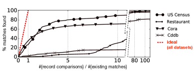
Figure 1: The performance of Progressive Sorted Neighborhood on 4 real-world structured datasets.

Our Contributions. We propose novel and unsupervised methods for Progressive ER that inherently address the Variety of Big Data: they operate in a schema-agnostic fashion, which overrides the need to search for and identify highly discriminative attributes, rendering schema knowledge unnecessary. Our methods are also more effective in addressing the Volume of Big Data, since they identify matches earlier than the top-performing schema-based method. They actually go beyond the state-of-the-art in Progressive ER by introducing and exploiting redundancy, i.e., by associating every profile with multiple blocking keys. Instead, existing schema-based progressive methods typically rely on highly discriminative attributes, which yield redundancy-free keys such that two profiles appear together in at most one block.

More specifically, our redundancy-based methods rely on two principles. The first one is called similarity principle, as it assumes that any two matching profiles have blocking keys that are closer in alphabetical order than those of non-matching ones. The second one is called equality principle, since it assumes that the matching likelihood of any two profiles is proportional to the number of blocks they share. Both principles have been successfully applied in Batch ER [7], but their application to the progressive context is non-trivial, as we show empirically. For this reason, we introduce more advanced methods for every principle.

Through an exhaustive experimental evaluation over 7 well-known datasets, we verify that similarity-based methods excel in structured datasets, outperforming even the state-of-the-art schema-based progressive method. These datasets typically involve a large portion of textual information, which provides reliable matching evidence when sorted alphabetically. In contrast, our equality-based method is the top-performer over semi-structured datasets (e.g., RDF data); it can exploit the semantics of the URIs that abound in this type of datasets, disregarding the useless information of URI prefixes, which introduce high levels of noise when sorted alphabetically.

On the whole, we make the following contributions:

$\bullet$ We introduce a schema-agnostic approach to Progressive ER, which inherently addresses the Variety of Big Data.

$\bullet$ We demonstrate that adapting existing schema-based methods to schema-agnostic Progressive ER is a non-trivial task: we introduce 2 naïve, schema-agnostic methods, showing experimentally that they fail to address the Volume issue of Big Data.

$\bullet$ We present 4 novel advanced, schema-agnostic progressive methods, which address both the Volume and the Variety of Big Data. They are classified in two categories: those based on a sorted list of profiles, leveraging the similarity principle, and those based on a graph of profiles, leveraging the equality principle.

$\bullet$ We perform a series of experiments over 7 established, real-world datasets, verifying experimentally the superiority of our methods over the existing schema-based state-of-the-art method, both in terms of effectiveness and time efficiency. We also investigate the relative performance of our methods, highlighting the top-performing ones, and providing guidelines for method selection.

The rest of the paper is structured as follows: Section 2 discusses the main works in the literature, while Section 3 describes the background of our methods. We present two naïve schema-agnostic solutions to Progressive ER in Section 4, and four advanced ones in Section 5. We elaborate on our extensive experimental evaluation in Section 7 and conclude the paper in Section 8, along with directions for future work.

2 Related Work

Schema-based Progressive Methods. The state-of-the-art progressive method is Progressive Sorted Neighborhood (PSN) [4, 5]. Based on Batch Sorted Neighborhood [8], it associates every profile with a schema-based blocking key. Then, it produces a sorted list of profiles by ordering all blocking keys alphabetically. Comparisons are progressively defined through a sliding window, $w$, whose size is iteratively incremented: initially, all profiles in consecutive positions ($w$=1) are compared, starting from the top of the list; then, all profiles at distance $w$=2 are compared and so on and so forth, until the processing is terminated.

However, the performance of PSN depends heavily on the attribute(s) providing the schema-based blocking keys that form the sorted list(s) of profiles. In case of low recall, the entire process is repeated, using multiple blocking keys per profile. As a result, PSN requires domain experts, or supervised learning on top of labeled data in order to achieve high performance. In contrast, our methods are completely unsupervised and schema-agnostic.

Two more schema-based methods were proposed in [5]: Hierarchy of Record Partitions (HRP) and Ordered List of Records (OLR). The main idea of HRP is to build a hierarchy of blocks, such that the matching likelihood of two profiles is proportional to the level in which they appear together for the first time: the blocks at the bottom of the hierarchy contain the profiles with the highest matching likelihood, and vice versa for the top hierarchy levels. Thus, the hierarchy of blocks can be progressively resolved, level by level, from the leaves to the root. This approach has been improved in the literature in two ways: (i) OLR exploits this hierarchy in order to produce a list of records sorted by their likelihood to produce matches, involving a lower memory consumption than HRP at the cost of a slightly worse performance. (ii) A schema-based variation of HRP is adapted to the MapReduce parallelization framework for even higher efficiency in [9]. It divides every block into a hierarchy of child blocks and uses an advanced strategy for optimizing their parallel processing.

However, both HRP and OLR are difficult to apply in practice. The hierarchies that lie at their core can be generated only when the distance of two records can be naturally estimated through a certain attribute (e.g., product price) [5]. The number of the hierarchy layers, $L$, has to be determined a-priori, along with $L$ similarity thresholds and the similarity measure that compares attribute values. Moreover, they both exhibit a performance inferior to PSN [5]. For these reasons, we do not consider these two methods any further.

Altowim et al. [10] propose a progressive joint solution in the context of multiple datasets containing different entity types. Similarly, in joint ER [11], the result on one dataset can be exploited to resolve the others. As an example, let us consider a joint ER on a movie dataset and on an actor dataset: discovering matches among actors can help to determine whether two movies associated to those actors are matching too (and vice versa). Both approaches, though, are only applicable to Relational ER.

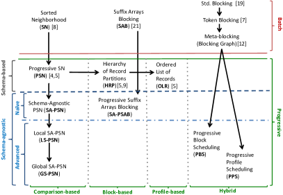
Figure 2: Overview of all discussed progressive methods. $A{\rightarrow}B$ means that method $B$ builds on method $A$ in order to offer a new functionality.

Taxonomy of Progressive Methods. We now present a taxonomy that organizes the existing progressive methods and those presented in the following with respect to the granularity of their functionality. This results in four categories, which generalize the hint types discussed in [5]:

(1) Comparison-based methods provide a list of profile pairs (i.e., comparisons) that are sorted in descending order of matching likelihood (from the highest to the lowest one). With every method call, these profile pairs are then emitted, one at a time, following that ordered list. This category is a generalization of the category “sorted list of record pairs” [5] and includes the methods PSN [4, 5], SA-PSN (see Section 4.1), LS-PSN (see Section 5.1.1), and GS-PSN (see Section 5.1.2).

(2) Block-based methods produce a list of blocks that are sorted in descending order of the likelihood that they include duplicates among their profiles. In every call, all the comparisons for each block are generated, one block at a time, following that ordered list; all comparisons in the same block have the same matching likelihood. This is a generalization of the category “hierarchy of record partitions” [5] and includes the homonymous method HRP [5] together with SA-PSAB (see Section 4.2).

(3) Profile-based methods provide a list of profiles that are sorted in descending order of duplication likelihood. Then, in every call, all comparisons of every entity are generated, one entity at a time, following that ordered list. This category is a generalization of the category “ordered list of records” [5] and includes the homonymous method OLR [5].

(4) Hybrid methods combine characteristics from two or all of the previous categories. This category includes PBS (see Section 5.2.1), which involves both block- and comparison-based characteristics, as well as PPS (see Section 5.2.2), which combines comparison-based characteristics with profile-based ones.

We illustrate our taxonomy in Figure 2, where every column corresponds to a different type of granularity (horizontal axis). On the vertical axis, we consider the relation of every progressive method to schema knowledge, with the topmost part corresponding to batch methods. Every arrow from method $A$ to method $B$ means that $B$ extends $A$ to offer a new functionality. For instance, PBS and PPS are based on the Blocking Graph, which is the core data structure of Batch Meta-blocking [12].

Crowdsourced (or Oracle) Methods. In Crowdsourced ER [13], humans are asked to label candidate profile pairs as either matching or non-matching, i.e., they are asked to behave like a binary match function. Such a function is typically assumed to be perfect (i.e., being equivalent to an oracle [14]) and transitive [15]. For example, given three profiles ($p_{1}$, $p_{2}$, $p_{3}$), if the crowd finds that $p_{1}$ matches with $p_{2}$, and $p_{2}$ with $p_{3}$, then the comparison between $p_{1}$ and $p_{3}$ is not crowdsourced, but is automatically deduced as a match. Progressive crowdsourced methods [15, 14, 16] exploit this transitivity to maximize the progressive recall of ER. In this work, though, we propose general methods for Progressive ER that are independent of the employed match function, i.e., we do not assume the match function to be transitive, nor to be perfect—a setting that is common for (non-crowdsourced) match functions [17]. We exclusively consider progressive methods that define a static processing order, without relying on the feedback of the “match function” to dynamically re-adjust it, as in crowdsourced methods or the “look-ahead strategy” that lies at the core of [4].

3 Preliminaries

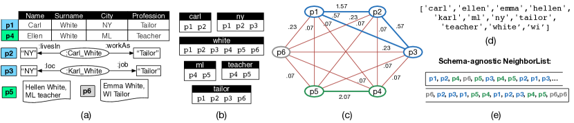
Figure 3: (a) A set of profiles $P$ that is extracted from a data lake with a variety of data formats: structured/relational data ($p_{1}$, $p_{4}$), semi-structured/RDF data ($p_{2}$, $p_{3}$) and unstructured/free-text data ($p_{5}$, $p_{6}$). Note that $p1{\equiv}p2{\equiv}p3$ and $p4{\equiv}p5$. (b) The block collection $B$ derived from $P$ by applying Token Blocking [18] to its profiles. (c) The Blocking Graph derived from $B$, with every edge representing a profile comparison that is weighted by the ARCS function. (d) The sorted list of attribute value tokens that appear in the profiles of $P$. (e) The corresponding schema-agnostic Neighbor List.

At the core of ER lies the notion of entity profile (or simply profile), which constitutes a uniquely identified set of attribute name-value pairs. An individual profile is denoted by $p_{i}$, with $i$ standing for its id in a profile collection $P$. Two profiles $p_{i},p_{j}\in P$ are called duplicates or matches ($\mathbf{p_{i}\equiv p_{j}}$) if they represent the same real-world entity.

Depending on the input data, ER takes two forms [1, 2]: (1) Clean-clean ER receives as input two duplicate-free, but overlapping profile collections, $P_{1}$ and $P_{2}$, and returns as output all pairs of duplicate profiles they contain, $P_{1}\cap P_{2}$. (2) Dirty ER takes as input a single profile collection that contains duplicates in itself and produces a set of equivalence clusters, with each one corresponding to a distinct profile.

To scale ER to large data collections, blocking is employed to cluster similar profiles into blocks so that it suffices to consider comparisons among the profiles of every block [19]. Each profile is indexed into blocks according to one or more criteria called blocking keys. If a blocking key depends on the schema(ta) of the data, we call it schema-based, otherwise schema-agnostic.

An individual block is symbolized by $b_{i}$, with $i$ corresponding to its id. The size of $b_{i}$ (i.e., the number of profiles it contains) is denoted by $|b_{i}|$ and its cardinality (i.e., the number of comparisons that it yields) by $\|b_{i}\|$. For instance, in Figure 3(b), $|b_{tailor}|{=}4$ and $\|b_{tailor}\|{=}{4\choose 2}{=}6$. A set of blocks $B$ is called block collection, with $|B|$ standing for its size (i.e., total number of blocks) and $\|B\|$ for its aggregate cardinality (i.e., the total number of comparisons entailed by $B$): $\|B\|$=$\sum_{b_{i}\in B}\|b_{i}\|$. The set of blocks associated with a specific profile $p_{i}$ is denoted by $B_{i}$, and the average number of profiles per block by $\mathbf{\bar{|b|}}$=$\sum_{b\in B}{|b|}/{|B|}$. The comparison between profiles $p_{i}$ and $p_{j}$ is symbolized by $c_{ij}$.

3.1 Progressive ER

In Batch ER, the profile comparisons entailed in block collection $B$ are executed without a specific order. Let $T_{o}$ be the overall time required for performing Batch ER on $B$. Based on $T_{o}$, Progressive ER is formally defined by two requirements [4, 5]:

$\bullet$ Improved Early Quality. If both Progressive and Batch ER are applied to $B$ and terminated at the same time $t{\ll}T_{o}$, then the former should detect significantly more matches than the latter.

$\bullet$ Same Eventual Quality. The result produced at time $T_{o}$ by Progressive and Batch ER should be identical. Even though progressive methods rarely run for so a long time as $T_{o}$, this requirement ensures their correctness, verifying that they yield the exact same outcome as batch methods.

In the following, we break the functionality of progressive methods into two phases:

(1) The initialization phase takes as input the profiles to be resolved, builds the data structures needed for their processing, and processes them to produce the overall best comparison.

(2) The emission phase returns the next best comparison from a list of candidates that are ranked in non-increasing order of matching likelihood. In other words, it identifies the remaining pair of profiles that has the highest matching likelihood.

By definition, the initialization phase is activated just once, while the emission phase is repeated whenever a new comparison is requested for processing.

3.2 Core Data Structures

We now describe two fundamental data structures for our progressive methods: the Blocking Graph and the Neighbor List. Every method discussed in the following has at its core either the former or the latter. Note that both data structures are known from the literature, sometimes with different names (e.g., the Neighbor List is called sorted list of records in [5]).

Blocking Graph — This data structure lies at the core of Batch Meta-blocking [1, 2, 12, 20], which aims at restructuring an existing block collection $B$ into a new one $B^{\prime}$ that has similar recall, but significantly higher precision than $B$. Meta-blocking relies on the assumption that the matching likelihood of any two profiles is analogous to their degree of co-occurrence in a block collection. This means that $B$ has to be generated by a blocking method that yields redundancy-positive blocks, where the similarity of two profiles is proportional to the number of blocks they share.

Based on redundancy, which is common for schema-agnostic blocking methods [12], Meta-blocking represents the block collection as a blocking graph. This is an undirected weighted graph $\mathcal{G}_{B}(V_{B},E_{B})$, where $V_{B}$ is the set of nodes, and $E_{B}$ is the set of weighted edges. Every node $n_{i}\in V_{B}$ represents a profile $p_{i}\in P$, while every edge $e_{i,j}$ represents a comparison $c_{i,j}\in B\subseteq P\times P$. A schema-agnostic weighting function is employed to weight the edges, leveraging the co-occurrence patterns of profiles in $B$: each edge is assigned a weight that is derived exclusively from the (characteristics of the) blocks its adjacent profiles have in common. For example, the ARCS function sums the inverse cardinality of common blocks, assigning higher scores to pairs of profiles sharing smaller (i.e., more distinctive) blocks: $ARCS(p_{i},p_{j},B)=\sum_{b_{k}\in B_{i}\cap B_{j}}1/\|b_{k}\|$. Similarly, all other weighting functions [12, 20] assign high weights to edges connecting profiles with strong co-occurrence patterns and low weights to casual co-occurrences.

Example 1.

Figure 3a shows a set of entity profiles, $P$. Figure 3b illustrates the block collection that is generated by applying Token Blocking to $P$, i.e., by creating a separate block for every token that appears in any attribute value of the input profiles (these tokens are called attribute value tokens in the following). Figure 3c depicts the Blocking Graph that is derived from the blocks of Figure 3b, when using the ARCS function for edge weighting.

Note that materializing and sorting all edges of a blocking graph is impractical for large datasets, due to the resulting huge graph size (i.e., the number of edges it contains) [12]. For this reason, all existing Meta-blocking methods [12, 20] discard low-weighted edges through a pruning algorithm, while building the Blocking Graph. As a result, they retain only the most promising comparisons, which are collected and employed for Batch ER. Based on such a Blocking Graph, we present in Section 5.2 a novel algorithm that generates comparisons in a progressive way.

Neighbor List — The Neighbor List is the core data structure of Sorted Neighborhood [8] and its derived methods (i.e., PSN [4, 5]). It is a list of profiles that is generated by sorting all profiles alphabetically, according to the blocking keys that represent them. This data structure is exploited to generate comparisons under the assumption that the matching likelihood of any two profiles is analogous to their proximity after sorting.

The Neighbor List can be built from schema-based [19] or from schema-agnostic [7] blocking keys and is typically employed to generate blocks: a window slides over the Neighbor List, and blocks correspond to groups of profiles that fall into the same window. The size of the window is iteratively incremented. The resulting blocks are called redundancy-neutral blocks, because the similarity of two profiles is not related to the number of blocks they share; the corresponding blocking keys might be close when sorted alphabetically, but rather dissimilar.

Example 2.

To understand the notion of redundancy-neutral blocks, consider the sorted schema-agnostic blocking keys (i.e., the attribute value tokens) of the profiles in Figure 3a, which are depicted in Figure 3d. The keys ‘carl’ and ‘ellen’ are placed in consecutive positions, but the corresponding profiles have nothing in common. Figure 3e shows the Neighbor List that corresponds to this sorted list of schema-agnostic blocking keys.

Note that in the schema-agnostic Neighbor List, every profile typically has multiple placements (e.g., once for each attribute value token) [7]. Hence, multiple distances can be measured for any pair of matching profiles. In Section 5.1, we present two approaches that leverage this phenomenon to improve the early quality of Progressive ER.

4 Naïve Methods

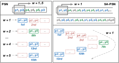
(a)                                  (b)

Figure 4: Progressive emission of comparisons for (a) PSN, and (b) SA-PSN; dashed boxes indicate non-matching comparisons.

Schema-based progressive methods (see Section 2) are hard to apply in a domain like Web data, where Variety renders the selection of schema-based blocking keys into a non-trivial task. Yet, we can convert the state-of-the-art schema-based progressive method (PSN) into a schema-agnostic one with minor modifications, as explained in Section 4.1. We can also adapt the established batch blocking method (Suffix Array Blocking [21, 19, 7]) into a progressive method, based on the ideas of HLR [9, 5], as explained in Section 4.2. However, our experimental analysis (Section 7) shows that both methods have inherent limitations that lead to poor performance, thus calling for the development of more advanced schema-agnostic progressive methods.

4.1 Schema-Agnostic PSN (SA-PSN)

The gist of this approach is to combine the sliding window with incremental size of PSN [5] with the Neighbor List of the schema-agnostic Sorted Neighborhood [7]. The resulting method is called Schema-Agnostic Progressive Sorted Neighborhood (SA-PSN).

Inevitably, the Neighbor List of SA-PSN may involve consecutive places with the same profile (i.e., a profile which contains two alphabetically consecutive tokens), or two profiles from the same source. The same applies to entire windows. For this reason, the comparisons extracted from every window should involve different profiles (Dirty ER), or profiles stemming from different sources (Clean-clean ER).

Example 3.

Figure 4 applies PSN and SA-PSN to the profiles of Figure 3a. For PSN, we assume that the schema of $p_{1}$ and $p_{4}$ describes all other profiles, even $p5$ and $p6$, which represent unstructured data and would require an information extraction preprocessing step. This assumption allows for defining a schema-based blocking key that concatenates the surname and the first two letters of the name. In this context, PSN in Figure 4a starts by emitting all comparisons produced by the initial window size, $w=1$; then, it continues with those comparisons entailed by window $w=2$ etc. The final pair of matches is emitted during the $15^{th}$ comparison, i.e., after raising the window size to $w=5$. In Figure 4b, SA-PSN applies the same procedure to the schema-agnostic Neighbor List, finding all matching profiles within the initial window frame $w=1$, after the $14^{th}$ comparison.

The main advantage of SA-PSN is that it involves a parameter-free functionality that requires no schema-based blocking key definition and has low space and time complexities (see Section 6). On the flip side, SA-PSN may perform repeated comparisons: the same pair of profiles might co-occur multiple times in the various windows. For example, in Figure 4b, $c_{12}$ is emitted as the $1^{st}$ and the $9^{th}$ comparison within the same window frame, $w=1$. Moreover, the proximity of two profiles in the list may be partially random; if more than two profiles share the same blocking key, they are inserted with a relatively random order in the Neighbor List. We call this phenomenon coincidental proximity. As an example, consider all 6 profiles in Figure 4b that are associated with the token white; they are placed in random order at the end of the Neighbor List. Note that PSN also suffers from coincidental proximity, which is a critical point to consider when devising the schema-based blocking keys.

4.2 Schema-Agnostic Progressive SAB (SA-PSAB)

Suffix Arrays Blocking (SAB) is a schema-based blocking technique that addresses noise at the start of blocking keys by converting them into all suffixes that contain at least $l_{min}$ characters (minimum suffix length) [21, 19]. Basically, SAB uses these suffixes to generate hierarchical blocks such that: the lowest levels in the hierarchy correspond to blocks generated with the initial blocking keys (e.g., “coin”, “join”, “pain”, ”gain”), the intermediate levels correspond to blocks generated with the intermediate suffixes (e.g., “oin”, “ain”), and the highest levels correspond to blocks generated with the shortest allowed suffixes (e.g., “in” for $l_{min}$=2). This hierarchy of blocks follows the corresponding hierarchies of suffixes, which we call suffix forest. Notice that there are as many suffix trees as the number of distinct suffixes of size $l_{min}$. Figure 5 depicts an example of suffix tree. To address the Variety of Big Data in a schema-agnostic fashion, every attribute value token can be considered as a blocking key [7].

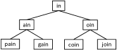
Figure 5: An example of a suffix tree employed by SA-PSAB.

The processing of an individual suffix tree follows a “leaves first, root last” approach.This means that the candidate pairs that appear in a lower level block (e.g., in a “leaf block”) are emitted before candidate pairs in a higher level block (e.g., a “root block”). Thus, for the entire suffix forest, the processing starts from the leaf node of the lowest layer (i.e., the overall largest attribute value token) and moves on to the tree roots; nodes of the same layer are ordered in increasing number of comparisons (i.e., the smallest nodes are processed first). We call the resulting method Schema-Agnostic Progressive Suffix Arrays Blocking (SA-PSAB).

Despite its complex functionality, SA-PSAB is probably the easiest-to-configure HRP or OLR progressive method. Its data-driven functionality simply extracts from every profile all attribute value tokens and for every such token, it considers as blocking keys all suffixes with at least $l_{min}$ characters. Therefore, $l_{min}$ is the only configuration parameter of SA-PSAB. Note also that SA-PSAB can be considered as the schema-agnostic version of the hierarchical progressive method proposed in [9].

5 Advanced Methods

We now introduce more elaborate methods for schema-agnostic Progressive ER, using a broad spectrum of techniques. We distinguish them into two categories: the similarity-based ones (Section 5.1), which employ a weighted Neighbor List, and the equality-based ones (Section 5.2), which employ a Blocking Graph. The former are based on the similarity principle, the latter on the equality principle (see Section 1).

Note that all our methods employ a data structure called Comparison List, which essentially constitutes a list of comparisons sorted in non-increasing order of matching likelihood. Its purpose is to store the best comparisons that were detected during the initialization phase so that they are efficiently emitted during the emission phase. Whenever the Comparison List gets empty, it is refilled with the next batch of the best remaining comparisons, during the next emission phase.

5.1 Similarity-based Methods

These methods extend the similarity principle of SA-PSN, assuming that the closer the blocking keys of two profiles are, when sorted alphabetically, the more likely they are to be matching. As explained above, SA-PSN suffers from two drawbacks: it contains numerous repeated comparisons and it defines a processing order of comparisons that is partially random, due to coincidental proximity. To address both disadvantages, we propose the use of a weighted Neighbor List, which employs a weighting scheme in order to associate every comparison with a numerical estimation of the likelihood that it involves a pair of matching profiles. This weighting scheme leverages the Neighbor List, with a functionality that is both schema- and domain-agnostic. Consequently, our approach addresses inherently the Variety of Web data.

To this end, we propose the Relative Co-occurrence Frequency (RCF) weighting scheme. RCF counts how many times a pair of profiles lies at a distance of $w$ positions in the Neighbor List and then normalizes it by the number of positions corresponding to each profile. To efficiently implement RCF and weighted Neighbor List, we go beyond Neighbor List by introducing a new data structure called Position Index. In essence, this is an inverted index that associates every profile (id) with its positions in the Neighbor List. Thus, it is generic enough to accommodate any weighting scheme that similarly to RCF relies on the co-occurrence frequency of profile pairs.

Below, we present two algorithms that exploit the RCF weighting scheme. Both of them are compatible with any other schema-agnostic weighting scheme that infers the similarity of profiles exclusively from their co-occurrences in the incremental sliding window. The core idea of these algorithms is to trade a higher computational cost of the initialization phase, and probably the emission phase, for a significantly better comparison order.

5.1.1 Local Schema-Agnostic PSN (LS-PSN)

This approach applies the selected weighting scheme only to the comparisons of a specific window size, thus defining a local execution order. At its core lie two data structures:

i) $NL$, which is an array that encapsulates the Neighbor List such that $NL[i]$ denotes the profile id that is placed in the $i^{th}$ position of the Neighbor List. An exemplary $NL$ array is shown in Step 1.i of Figure 6.

ii) $PI$, which stands for Position Index, is an inverted index that points from profile ids to positions in $NL$. It is implemented with an array that uses profile ids as indexes, such that $PI[i]$ returns the list of the positions associated with profile $p_{i}$ in $NL$. This array accelerates the estimation of comparison weights, since it minimizes the computational cost of retrieving the neighbors of any profile in the current window, as described below. Note that instead of a Position Index, LS-PSN could use a hash index that has comparisons as keys and weights as values. This approach, however, would increase both the space and the time complexity of comparison weighting.

Input: (i) Profile collection $P$, (ii) Weighting scheme, $wScheme$

Output: The overall best comparison

1 $windowSize$ = 1;

2 $ComparisonList$ $\leftarrow$ $\emptyset$;

3 $NL$[] $\leftarrow$ buildNeighborList($P$);

4 $PI$[] $\leftarrow$ buildPositionIndex($NL$[]);

5 foreach $p_{i}$ $\in$ $P$ do

6       $distinctNeighbors$ $\leftarrow$ $\emptyset$; // a set containing distinct neighbors;

7       $frequency$[] $\leftarrow$ $\emptyset$;

8       foreach $position$ $\in$ $PI$[$i$] do

9             $p_{j}$ $\leftarrow$ $NL$[$position$+$windowSize$];

10             if isValidNeighbor($p_{j}$) then

11                   $frequency$[$j$]++;

12                   $distinctNeighbors$.add($j$);

13                  

14            

15            $p_{k}$ $\leftarrow$ $NL$[$position$-$windowSize$];

16             if isValidNeighbor($p_{k}$) then

17                   $frequency$[$k$]++;

18                   $distinctNeighbors$.add($k$);

19                  

20            

21      

22      foreach $j$ $\in$ $distinctNeighbors$ do

23             $weight_{i,j}$ $\leftarrow$ $wScheme$($frequency$[$j$], $j$, $i$);

24             $ComparisonList$.add(getComparison($i$, $j$, $weight_{i,j}$);

25            

26      

27

28sortInDescreasingWeight($ComparisonList$);

29

30return $ComparisonList$.removeFirst();

Algorithm 1 Initialization phase for LS-PSN.

Output: The next best comparison

1 while $ComparisonList$.isEmpty() do

2       $windowSize$++;

3       if $NL$.size() $<$ $windowSize$  then

4             return null;

5            

      /* repeat lines 5 - 20 in Algorithm 1 */

6      

7return $ComparisonList$.removeFirst();

Algorithm 2 Emission phase for LS-PSN.

Based on these data structures, the initialization phase of LS-PSN is outlined in Algorithm 1. Initially, it sets the window size to 1 (Line 1), considering only consecutive profiles. Then, it creates its data structures (Lines 2-4) and for every profile $p_{i}$ (Line 5), it iterates over all its positions in the Position Index (Line 8). In every position, LS-PSN checks the neighbors in both directions, i.e., the profiles located $windowSize$ places before and after $p_{i}$ (Lines 13 and 9, respectively) - provided that the corresponding positions are within the limits of the Neighbor List. For every neighbor $p_{j}$, LS-PSN checks if $j{<}i$ (Line 10) and $k{<}i$ (Line 14) to avoid repeated comparisons. For every valid neighbor, LS-PSN increases its frequency (Lines 11 and 15) and adds it into the set of neighbors (Lines 12 and 16). Then, the overall weight for every comparison is computed according to the selected weighting scheme (Line 18) - assuming a comparison between $p_{i}$ and $p_{j}$, i.e., $c_{i,j}$, the corresponding RCF weight is equal to $\frac{frequency[j]}{PI[i].length()+PI[j].length()-frequency[j]}$. Finally, all comparisons are aggregated and sorted from the highest weight to the lowest (Line 20) and the top one is returned (Line 21).

Note that Algorithm 1 pertains to Dirty ER. Yet, it can be adapted to Clean-clean ER with two minor modifications: (i) Line 5 iterates over the profiles of $P_{1}$, and (ii) in Lines 10 and 14, a neighbor $p_{j}$ is considered valid only if $p_{j}\in P_{2}$.

The emission phase of LS-PSN is illustrated in Algorithm 2 and is common for both Clean-clean and Dirty ER: if the Comparison List corresponding to the current window is not empty, the top weighted one is removed and returned as output (Line 3). If the list is empty, the window size is incremented (Line 2) and the process for extracting all comparisons of the new window (Lines 5 - 20 in Algorithm 1) is repeated. After each emission, the processing can be interrupted. In the worst case, the emission phase is terminated when the window size is equal to the size of the Neighbor List (Lines 3-4). This means that the window is so large that it ends up comparing every profile with all others.

Example 4.

We demonstrate the functionality of LS-PSN by applying it to the profiles of Figure 3a. The result appears in Figure 6. Step 0 extracts all blocking keys and sorts them alphabetically, while Step 1.i forms $NL$ and slides a window of size 1 over it. In Step 1.ii, we see the result of the nested loops in Lines 5 - 16 for the RCF weighting scheme for $windowSize$=1. In Step 1.iii, all comparisons are weighted and sorted from the highest to the lowest weight. Finally, the sorted comparisons are emitted one by one in Step 1.iv. Note that the first three comparisons correspond to the three pairs of duplicate profiles.

5.1.2 Global Schema-Agnostic PSN (GS-PSN)

The main drawback of LS-PSN is the local execution order it defines for a specific window size. This means that LS-PSN is likely to emit the same comparison(s) multiple times, for two or more different window sizes, since it does not remember past emissions. GS-PSN aims to overcome this drawback by defining a global execution order for all the comparisons in a range of window sizes $[1,w_{max}]$. To this end, its initialization phase differs from Algorithm 1 in that Line 1 is converted into an iteration over all window sizes in $[1,w_{max}]$; this loop starts before Line 8 and ends before Line 20. This allows for a simpler emission phase, which just returns the next best comparison, until the Comparison List gets empty.

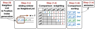
Figure 6: Applying LS-PSN to the profiles of Figure 3a.

Compared to LS-PSN, GS-PSN takes into account more co-occurrence patterns, when determining comparison weights. Consequently, its matching likelihood estimations are expected to be more accurate than those of LS-PSN. This is achieved through an additional configuration parameter, $w_{max}$, which eliminates all repeated comparisons in a particular range of windows.

5.2 Equality-based Methods

These methods rely on the equality principle of the redundancy-positive blocks that are derived from any schema-agnostic blocking method or workflow [12]: they assume that the more blocks two entities share, the more likely they are to be matching. From these blocks, we extract the Blocking Graph of Meta-blocking, using the weights of its edges as approximations for the matching likelihood of the corresponding comparison. In particular, we order the graph edges in decreasing weight in order to produce a sorted list of comparisons at the level of individual blocks or profiles. Below, we propose two novel algorithms of this type.

5.2.1 Progressive Block Scheduling (PBS)

This algorithm is specifically designed for Progressive ER, but relies on a Batch ER technique. Indeed, Block Scheduling has been proposed in order to optimize the processing order of blocks in the context of Batch ER, based on the probability that they contain duplicates [1]. It assigns to every block a weight that is proportional to the likelihood that it contains duplicates and then, it sorts all blocks in descending weight order. Even though we would like to use such a functionality for Progressive ER, it is not applicable, because: (i) its weighting cannot generalize to Dirty ER, applying exclusively to Clean-clean ER, and (ii) it does not specify the execution order of comparisons inside blocks with more than two profiles.

Our algorithm, PBS, deals with both issues in two ways:

(1) PBS introduces a weighting mechanism that applies uniformly to Clean-clean and Dirty ER. In fact, it relies on the reasonable hypothesis that the smaller a block is, the more distinctive information it encapsulates and the more likely it is to contain duplicate profiles, and vice versa: the larger a block is, the more frequent is the corresponding blocking key/token and the more likely it corresponds to a stop word, thus ingesting noise into the matching likelihood of two entities. Therefore, our scheme sets weights inversely proportional to block cardinalities (i.e., $1/\|b_{i}\|$) and sorts blocks in decreasing weights; the fewer comparisons a block entails, the higher it is ranked.

(2) PBS defines the processing order of comparisons inside every block using the Blocking Graph. For each block $b_{i}$ with $\|b_{i}\|$$>$$1$, PBS associates all comparisons with a weight derived from any schema-agnostic weighting scheme of Meta-blocking. Then, it sorts them from the highest weight to the lowest one.

It is worth noting that all repeated comparisons are discarded before computing their weight. In fact, the efficient detection of repeated comparisons is crucial for PBS. This functionality is based on a data structure called Profile Index, which constitutes an inverted index that associates every profile with the ids of the blocks that contain it. In this way, it facilitates the efficient computation of comparison weights, similar to the Position Index of LS/GS-PSN. Note that the Profile Index is generic enough to accommodate any weighting scheme that is based on the block co-occurrence frequency of profile pairs.

In practice, the Profile Index is implemented as a two-dimensional array. The first dimension is of size $|P|$ such that $ProfileIndex[i]$ points to an array that contains all ids of the blocks involving profile $p_{i}$. As a result, the second dimension contains arrays of variable length. The block ids in every such array are sorted from the lowest to the highest one in order to ensure high efficiency for the two operations that are built on top of the Profile Index.

Input: (i) Profile collection $P$, (ii) Weighting scheme, $wScheme$

Output: The overall best comparison

1 $B$ $\leftarrow$ buildRedundancyPositiveBlocks($P$);

2 $B^{\prime}$ $\leftarrow$ blockScheduling($B$);

3 $ProfileIndex$ $\leftarrow$ buildProfileIndex($B^{\prime}$);

4 $b_{k}$ $\leftarrow$ $B^{\prime}$.removeFirst();

5 $ComparisonList$ $\leftarrow$ $\emptyset$;

6 foreach $c_{ij}$ $\in$ $b_{k}$ do

7       $B_{i}$ $\leftarrow$ $ProfileIndex$.getBlocks($p_{i}$);

8       $B_{j}$ $\leftarrow$ $ProfileIndex$.getBlocks($p_{j}$);

9       if nonRepeated($k$, $B_{i}$, $B_{j}$) then

10             $w_{i,j}$ $\leftarrow$ $wScheme$($k$, $B_{i}$, $B_{j}$);

11             $ComparisonList$.add(getComparison($i$, $j$, $w_{i,j}$));

12            

13      

14sortInDescreasingWeight($ComparisonList$);

15

16return $ComparisonList$.removeFirst();

Algorithm 3 Initialization phase for PBS.

Output: The next best comparison

1 if $ComparisonList$.isEmpty() then

       /* repeat lines 4 - 12 in Algorithm 3 */

2      

3return $ComparisonList$.removeFirst();

Algorithm 4 Emission phase for PBS.

The first operation is the Least Common Block Index (LeCoBI) condition, which checks whether a comparison is repeated in Line 9 of Alg. 3: given a comparison $c_{ij}$ in block $b_{Y}$, the LeCoBI condition identifies the least common block id, X, between the profiles $p_{i}$ and $p_{j}$ and compares it with the id of $b_{Y}$, Y. If the two ids match ($X=Y$), $c_{ij}$ corresponds to a new comparison. Otherwise $X<Y$, which means that $c_{ij}$ has already been compared in block $b_{X}$, but is repeated in block $b_{Y}$. Note that $X>Y$ is impossible, because the id of every block indicates its position in the processing list after sorting all blocks in increasing cardinalities (i.e., $b_{k}$ denotes the block placed in the $k^{th}$ position after sorting). Note also that by ordering the block ids of the second dimension in increasing order, the Profile Index minimizes the checks required for detecting the least common block id, thus accelerating the LeCoBI condition.

The second operation is Edge Weighting, which in Line 10 of Alg. 3 infers the matching likelihood of every comparison from the weight of the corresponding edge in the blocking graph. Given a non-repeated comparison $c_{ij}$, it compares the block lists associated with profiles $p_{i}$ and $p_{j}$ in order to estimate the number of blocks they share. This number, which lies at the core of practically all Meta-blocking weighting schemes [12], can be derived from the evidence provided by the Profile Index. Note that by ordering the block ids of its second dimension in increasing order, the Profile Index allows for accelerating Edge Weighting by traversing the two block lists in parallel.

On the whole, the initialization phase of PBS appears in Algorithm 3. Initially, it creates a redundancy-positive block collection and sorts its elements in non-decreasing order of comparisons (Lines 1-2). Then, it builds the corresponding Profile Index (Line 3) and goes on to remove the first (i.e., smallest) block, iterating over its comparisons (Lines 4-6). For every comparison $c_{ij}$, PBS gets the block lists that are associated with profiles $p_{i}$ and $p_{j}$ from the Profile Index (Lines 7-8). Based on these lists, it evaluates the LeCoBI condition, checking whether $c_{ij}$ is repeated or not (Line 9). If $c_{ij}$ is a new comparison, it is placed in the Comparison List along with the weight of the corresponding Blocking Graph edge (Lines 10-11). After processing all comparisons in the current block, the elements of the Comparison List are sorted in decreasing weight and the first one is emitted (Lines 12-13).

The emission phase of PBS appears in Algorithm 4. If the Comparison List is empty, it processes the next block $b^{\prime}$$\in$$B^{\prime}$, applying the Lines 4-12 of Algorithm 3 to it. Otherwise, the next best comparison is emitted from the Comparison List.

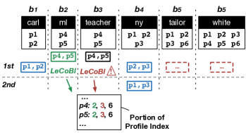
Figure 7: Applying PBS to the blocks of Figure 3b.

Example 5.

Figure 7 illustrates the functionality of PBS by applying it to the blocks of Figure 3b. First, it sorts them in non-decreasing cardinality and assigns to each one an incremental block id that indicates its processing order (note that we chose a random permutation of the blocks that have the same number of comparisons, without affecting the end result). Then, PBS processes the sorted list of blocks one block at a time, emitting iteratively the comparisons entailed in every block. Inside every block, all comparisons that satisfy the LeCoBl condition (i.e., non-repeated comparisons) are sorted according to the corresponding edge weight in the Blocking Graph of Figure 3c. For instance, when PBS processes $b_{2}$, the comparison $c_{45}$ satisfies the LeCoBl condition, since the least common block id shared by $p4$ and $p5$ is 2. This means that PBS encounters $c_{45}$ for the first time in $b_{2}$, assigning the edge weight 1.33 to it. In contrast, when PBS processes $b_{3}$, the comparison $c_{45}$ does not satisfy the LeCoBl condition anymore and is thus discarded.

5.2.2 Progressive Profile Scheduling (PPS)

The block-centric functionality of PBS is crafted for an Edge Weighting approach that operates at the level of individual comparisons. We now propose a novel progressive method with entity-centric functionality, called Progressive Profile Scheduling (PPS).

PPS is based on the concept of duplication likelihood, i.e., the likelihood of an individual profile $p_{i}$ to have matches. In Clean-clean ER, the duplication likelihood of $p_{i}\in P_{1}$ corresponds to its likelihood to have a match in $P_{2}$, since there can be up to one matching profile per entity in every profile collection. In Dirty ER, though, the duplication likelihood of $p_{i}$ is analogous to the size of its equivalence cluster, i.e., high values indicate that $p_{i}$ matches with many other profiles, and vice versa for low values.

In fact, PPS aims to sort all profiles in decreasing duplication likelihood, forming a data structure that is called Sorted Profile List. Then, moving from the top to the bottom of this list, PPS goes iteratively through every profile, emitting the top-$k$ weighted comparisons that entail it in decreasing matching likelihood.

To build the Sorted Profile List, PPS derives the duplication likelihood of every profile from a given Blocking Graph. The underlying assumption is the same as for all methods based on a Blocking Graph: the weight of a blocking graph edge captures the matching likelihood between the adjacent profiles. Thus, the duplication likelihood of each node (i.e., profile) is estimated by aggregating the weights of its incident edges. In particular, our implementation of PPS approximates the duplication likelihood of a profile through the average weight of the edges that are incident to the corresponding node - other aggregation functions can be employed instead, but the average one consistently exhibited high performance across different datasets.

Input: (i) Profile collection: $P$, (ii) Weighting scheme, $wScheme$

Output: The overall best comparison

1 $B$ $\leftarrow$ buildRedundancyPositiveBlocks($P$);

2 $ProfileIndex$ $\leftarrow$ buildProfileIndex($B$);

3 $SortedProfileList$ $\leftarrow$ $\emptyset$;

4 $topComparisonsSet$ $\leftarrow$ $\emptyset$;

5 foreach $p_{i}$ $\in$ $P$ do

6       $weights$[] $\leftarrow$ $\emptyset$;

7       $distinctNeighbors$ $\leftarrow$ $\emptyset$;

8       foreach $b_{k}$ $\in$ $ProfileIndex$.getBlocks($p_{i}$) do

9             foreach $p_{j}$($\neq$$p_{i}$) $\in$ $b_{k}$ do

10                   $weights$[$j$] += wScheme($p_{j}$, $p_{i}$, $b_{k}$);

11                   $distinctNeighbors$.add($j$);

12                  

13            

14      

15      $topComparison$ $\leftarrow$ $null$;

16       $duplicationLikelihood$ $\leftarrow$ 0;

17       foreach $j$ $\in$ $distinctNeighbors$ do

18             $duplicationLikelihood$ += $weights$[$j$];

19             if $topComparison$.getWeight() $<$ $weights$[$j$] then

20                   $topComparison$ $\leftarrow$ getComparison($i$, $j$, $weights$[$j$];

21                  

22            

23      $topComparisonsSet$.add($topComparison$);

24      

25      $duplicationLikelihood$ /= $distinctNeighbors$.size();

26       $SortedProfileList$.add($p_{i}$, $duplicationLikelihood$);

27      

28

29$ComparisonList$.addAll($topComparisonsSet$);

30 sortInDescreasingWeight($ComparisonList$);

31 sortInDescreasingWeight($SortedProfileList$);

32

33return $ComparisonList$.removeFirst();

Algorithm 5 Initialization phase for PPS.

Output: The next best comparison

1 $checkedEntities$ $\leftarrow$ $\emptyset$;

2 if $ComparisonList$.isEmpty() then

3       if $SortedProfileList$.isNotEmpty() then

4             $p_{i}$ = $SortedProfileList.removeFirst()$;

5             $checkedEntities$.add($i$);

6             $weights$[] $\leftarrow$ $\emptyset$;

7             $distinctNeighbors$ $\leftarrow$ $\emptyset$;

8             $SortedStack$ $\leftarrow$ $\emptyset$;

9             foreach $b_{k}$ $\in$ $ProfileIndex$.getBlocks($p_{i}$) do

10                   foreach $p_{j}$($\neq$$p_{i}$) $\in$ $b_{k}$ do

11                         if $checkedEntities$.contains($j$) then

12                               continue;

13                              

14                        $weights$[$j$] += wScheme($p_{j}$, $p_{i}$, $b_{k}$);

15                         $distinctNeighbors$.add($j$);

16                        

17                  

18            

19            foreach $j$ $\in$ $distinctNeighbors$ do

20                   $SortedStack$.push(getComparison($i$, $j$, $weights$[$j$]);

21                   if $K_{max}$ $<$ $SortedStack$.size() then

22                         $SortedStack$.pop();

23                        

24                  

25            $ComparisonList$ $\leftarrow$ sortInDescreasingWeight($SortedStack$);

26            

27      

28return $ComparisonList$.removeFirst();

Algorithm 6 Emission phase for PPS.

During the creation of the Sorted Profile List, PPS also initializes the Comparison List with the set of the top-weighted comparisons of each node. This step does not require any additional computational cost. While investigating the neighborhood of a particular node, PPS retains in a local variable the highest edge weight along with the corresponding comparison. After traversing all edges in the neighborhood, the overall best comparison is added to the set $topComparisonsSet$. As soon as all nodes have been processed, PPS sorts the elements of $topComparisonsSet$ in decreasing matching likelihood and adds them to the Comparison List. In the end, this process allows for emitting the comparison with the highest weight across the entire Blocking Graph, i.e., the comparison placed in the first position of the Comparison List.

In more detail, the initialization phase of PPS is outlined in Algorithm 5. First, a redundancy block collection is created along with the corresponding $ProfileIndex$ (Lines 1-2). Subsequently, PPS iterates over all input profiles (Line 5) and for every profile $p_{i}$, it goes through the blocks that contain it, $B_{i}$, which are derived from the Profile Index (Line 8). For every such block, it iterates over the co-occurring profiles, placing them into the set of neighbor ids and updating their overall weight (Lines 9-11). After examining all blocks, it goes through the set of neighbor profiles in order to estimate the overall duplication likelihood and identify the top-weighted comparison (Lines 12-17). The selected comparison is then added to the set of top-weighted comparisons, which makes sure that none of them is repeated, while the current profile is added to the Sorted Profile List along with its duplication likelihood (Lines 18-20). After processing all profiles, the top-weighted comparisons are added to the Comparison List to be sorted in decreasing order of weights; the same applies to Sorted Profile List (Lines 21-23). Finally, the overall top-weighted comparison is emitted (Line 24).

The emission phase of PPS relies on two pillars:

(i) A data structure called $SortedStack$, which contains a set of comparisons such that they are constantly sorted in non-decreasing weight, from the lowest to the highest one. Thus, its head always corresponds to the comparison with the lowest weight and can be efficiently removed with the a pop operation of constant computational cost, $O(1)$.

(ii) A custom mechanism for avoiding repeated comparisons that relies on a set with all entities that have already been processed, called $checkedEntities$. Before considering the comparison of the current profile $p_{i}$ with a co-occurring one $p_{j}$, $c_{ij}$, we investigate whether $checkedEntities$ contains the id $j$. If yes, $c_{ij}$ is skipped, based on the observation that the most important comparisons of $p_{j}$ have already been emitted. In this way, we disregard even comparisons that are among the $K_{max}$ top-weighted ones for the current entity, $p_{i}$, but not for the previously examined one, $p_{j}$. The reason is that $p_{j}$’s higher duplication likelihood provides more reliable evidence for $c_{ij}$’s low matching likelihood.

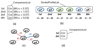
Figure 8: (a) The Comparison List after the initialization phase, containing the top-weighted comparison of every node in the Blocking Graph of Figure 3c. (b) The corresponding Sorted Profile List. (c) The node neighborhood of $p_{2}$ in the same Blocking Graph. (d) The Comparison List after processing $p_{2}$ during the emission phase.

TABLE I: Space and time complexities of our methods. In some cases, the emission phase complexity depends on the status of the Comparison List.

Method	Acronym	Space	Time complexity
		Complexity	Initialization Phase	Emission Phase
Schema-agnostic Progressive Sorted Neighborhood	SA-PSN	$O($$\mathbf{\bar{|p|}}$$\cdot$$|P|)$	$O($$\mathbf{\bar{|p|}}$$\cdot$$|P|$$\cdot$$\log$$(\mathbf{\bar{|p|}}$$\cdot$$|P|))$	$O(1)$
Schema-agnostic Progressive Suffix Arrays Blocking	SA-PSAB	$O($$\bar{s_{e}}$$\cdot$$|P|)$	$O($$\bar{s_{e}}$$\cdot$$|P|$$\cdot$$\log$$(\bar{s_{e}}$$\cdot$$|P|))$	$O(1)$
Global Scheam-agnostic Progressive Sorted Neighborhood	GS-PSN	$O(w_{max}$$\cdot$$\mathbf{\bar{|p|}}$$\cdot$$|P|)$	$O($$\mathbf{\bar{|p|}}$$\cdot$$|P|$$\cdot$$\log$$(\mathbf{\bar{|p|}}$$\cdot$$|P|))$	$O(1)$
Local Scheam-agnostic Progressive Sorted Neighborhood	LS-PSN	$O(\mathbf{\bar{|p|}}$$\cdot$$|P|)$	$O($$\mathbf{\bar{|p|}}$$\cdot$$|P|$$\cdot$$\log$$(\mathbf{\bar{|p|}}$$\cdot$$|P|$))	$O(1)$ or $O($$\mathbf{\bar{|p|}}$$\cdot$$|P|)$
Progressive Profile Scheduling	PPS	$O(\mathbf{\bar{|p|}}$$\cdot$$|P|)$	$O(|V_{B}|+|E_{B}|)$	$O(1)$ or $O(\mathbf{\bar{|p|}}$$\cdot$$\mathbf{\bar{|b|}})$
Progressive Block Scheduling	PBS	$O(\mathbf{\bar{|p|}}$$\cdot$$|P|)$	$O(|B|$$\cdot$$\log|B|)$	$O(1)$ or $O(\|\bar{b}\|$$\cdot$$\log\|\bar{b}\|)$

In more detail, the emission phase of PPS is outlined in Algorithm 6. Initially, it emits the top-weighted comparisons that were placed in the Comparison List during initialization. As soon as this list gets empty, PPS iterates over the individual profiles according to their duplication likelihood, from the highest to the lowest one (Lines 2-4). For the next available profile, PPS retrieves the associated blocks from the Profile Index (Line 9) and iterates over their contents in order to gather their $K_{max}$ top-weighted comparisons (Lines 10-19): initially, PPS goes through the co-occurring profiles, skipping the already examined ones (Lines 10-12). The non-examined ones are then added to the set of neighbor ids and their overall weight is updated (Lines 13-14). After examining all blocks, PPS estimates the overall weight for every neighbor, pushing the corresponding comparison in the sorted stack (Lines 15-16). If the size of the stack exceeds $K_{max}$, the comparison with the lowest weight is popped (Lines 17-18).

Finally, the remaining comparisons are sorted in decreasing weights and placed in the Comparison List (Line 19), followed by emission of the top-weighted comparison (Line 20).

Example 6.

To illustrate the functionality of PPS, consider the example in Figure 8. During the initialization phase, PPS iterates over all nodes of the Blocking Graph to compute the average weight of the incident edges along with the top-weighted comparison in every node neighborhood. At the end of this iteration, all top-weighted comparisons and all profiles are sorted in non-increasing weights, from the highest to the lowest one, in order to form the Comparison List in Figure 8a and the Sorted Profile List in Figure 8b, respectively. During the emission phase, PPS initially emits all comparisons in the Comparison List of Figure 8a. Then, it goes through the Sorted Profile List, one node at a time, gathering the top-k comparisons in the corresponding node neighborhood. For instance, Figure 8c shows the neighborhood of $p_{2}$, whose top-2 edges are inserted in the Comparison List of Figure 8d. Note that $p_{1}$ has already been processed, since it was placed first in the Sorted Profile List of Figure 8b. As a result, the control in Line 11 in Algorithm 6, checkedEntities.contains(1), returns true and $c_{12}$ is not inserted in the Comparison List of Figure 8d, despite its high edge weight.

6 Complexity Analysis

We now elaborate on the space and time complexities of all algorithms presented in Sections 4 and 5. All complexities are summarized in Table I.

6.1 Space Complexity.

We observe that for most methods, the space complexity is linear with respect to the size of the input dataset, $|P|$. For SA-PSN and LS-PSN, it is just $O($$\mathbf{\bar{|p|}}$$\cdot$$|P|)$, where $\mathbf{\bar{|p|}}$ is the average number of name-value pairs ($\sim$ blocking keys per entity), because they mainly keep in memory the Profile List. LS-PSN additionally maintains the Position Index, but it has exactly the same complexity. The same holds for the Profile Index, which dominates the space requirements of PPS and PBS. GS-PSN occupies more space, $O(w_{max}{\cdot}\mathbf{\bar{|p|}}{\cdot}|P|)$, due to the Comparison List, which, in the worst case, contains 1 comparison per position in the Profile List for every window size. To keep the suffix forest in memory, SA-PSAB has a space complexity of $O($$\bar{s_{e}}$$\cdot$$|P|)$, where $\bar{s_{e}}$ is the average number of suffixes per profile. Thus, we can conclude that all methods scale well to the Volume of Web data.

6.2 Time Complexity

Initialization phase. All methods are also scalable with respect to the time complexity of their initialization phase. For the similarity-based methods, SA-PSN, LS-PSN and GS-PSN, the time complexity is dominated by the sorting of blocking keys in alphabetical order, $O($$\mathbf{\bar{|p|}}$$\cdot$$|P|$$\cdot$$\log$$(\mathbf{\bar{|p|}}$$\cdot$$|P|))$. For SA-PSAB, it is $O($$\bar{s_{e}}$$\cdot$$|P|$$\cdot$$\log$$(\bar{s_{e}}$$\cdot$$|P|))$, as it sorts all suffixes (i.e., tree nodes) in non-increasing order of length and non-decreasing order of comparisons. For PPS, the initialization time complexity is $O(|V_{B}|+|E_{B}|)$, as this method iterates over all nodes and edges of the blocking graph $G_{B}$, without any pruning. Finally, the time complexity of PBS is dominated by the sorting of blocks in non-decreasing comparisons, i.e., $O(|B|{\cdot}\log|B|)$. Note that for both equality-based methods, the cost of building the block collection $B$ is insignificant, as it typically requires a single iteration over the input profiles, $O(|P|)$.

Emission phase. We distinguish all methods into three categories with respect to the time complexity of this phase. The first one includes the naïve methods, SA-PSN and SA-PSAB, which simply return the next comparison in a window or tree node, thus exhibiting a constant time complexity, $O(1)$. Yet, a large part of the emitted comparisons is repeated, as every profile is associated with multiple keys. Due to their simplicity, though, these methods make no provision for detecting repeated comparisons.

The second category includes GS-PSN, which exhibits a constant time complexity, $O(1)$, without emitting repeated comparisons. The reason is that it precomputes all comparisons, discarding the repeated ones.

The third category involves all methods with unstable response time, namely LS-PSN, PPS and PBS. In most cases, their time complexity is constant, but whenever their Comparison List gets empty, they renew its contents by repeating (part of) their initialization phase. In fact, the emission time complexity of LS-PSN is equal to that of the initialization phase, as the same process is applied to the entire Sorted Profile List; the only difference is the incremented window size. PBS also applies the same procedure as the initialization phase in order to refill its Comparison List. Yet, the time complexity is now much lower, as it is dominated by the sorting of all comparisons in an individual block, i.e., $O(\|\bar{b}\|$$\cdot$$\log\|\bar{b}\|)$, on average, rather than by the sorting of the entire block collection, $B$. Finally, the emission phase of PPS is significantly more efficient than its initialization phase: it merely sorts the comparisons associated with a single entity in non-increasing matching likelihood, $O($$\mathbf{\bar{|p|}}$$\cdot$$|P|)$, on average, instead of sorting all profiles in non-increasing duplication likelihood.

7 Experiments

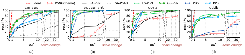
Figure 9: Recall progressiveness over the structured datasets.

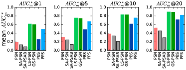
Figure 10: Mean $AUC_{m}^{*}$ over the structured datasets.

Datasets. For the experimental evaluation, we employ 7 diverse real-world datasets that are widely adopted in the literature as benchmark data for ER [19, 12, 20, 22, 23]. Their characteristics are reported in Table II. The census, restaurant, cora, and cddb datasets are extracted from a single data source containing duplicated profiles, hence they are meant to test Dirty ER tasks. The remaining datasets (movies, dbpedia, and freebase) are suitable for testing scalability, as well as Clean-clean ER, since they are extracted from two different data sources, where matching profiles exist only between a source and another: movies from imdb.com and dbpedia.org; dbpedia from two different snapshots of DBpedia (dbpedia.org 2007-2009); freebase from developers.google.com/freebase/ and dbpedia.org (extracted from [23]). For all the datasets, the ground truth is known and provided with the data.

TABLE II: Dataset characteristics: ER type, number of entity profiles ($|P|$), number of attribute names, number of existing matches ($|\mathcal{D}_{P}|$) and average number of name-value pairs per entity ($|\bar{p}|$).

	ER type	$|P|$	#attr.	$|\mathcal{D}_{P}|$	$|\bar{p}|$
Structured Datasets
census	Dirty ER	841	5	344	4.65
restaurant	Dirty ER	864	5	112	5.00
cora	Dirty ER	1.3k	12	17k	5.53
cddb	Dirty ER	9.8k	106	300	18.75
Large, Heterogeneous Datasets
movies	Clean-clean ER	28k—23k	4—7	23k	7.11
dbpedia	Clean-clean ER	1.2M—2.2M	30k—50k	893k	15.47
freebase	Clean-clean ER	4.2M—3.7M	37k—11k	1.5M	24.54

For the structured datasets, the best schema-based blocking keys for PSN are known from the literature [7, 19]. Note that the schema-based methods are inapplicable to the large, heterogeneous datasets. This is due to the size of the attribute set and the lack of a schema-alignment for Clean-clean datasets. Finally, in dbpedia and freebase, there is a very small overlap in the attributes describing their profile collections.

System setup. All methods are implemented in Java 8 and the code is publicly available. All experiments have been performed on a server running Ubuntu 14.04, with 80GB RAM, and an Intel Xeon E5-2670 v2 @ 2.50GHz CPU. Note that we limited the maximum heap size parameter of the JVM to 8GB for the structured datasets and for movies, while for DBPedia and Freebase we set that parameter to 80GB.

Parameter configuration. We apply the following settings to all datasets. For GS-PSN, we set $w_{max}$=20 for structured datasets and $w_{max}$=200 for large, heterogeneous datasets—preliminary experiments have shown that these values work for all the datasets. For PBS and PPS, we can use any schema-agnostic blocking method that produces redundancy-positive blocks, like DisNGram [24].

We opted for the Token Blocking Workflow, which has been experimentally verified to address effectively and efficiently the Volume and Variety of Web data [12]. It consists of the following steps: (1) Schema-agnostic Standard Blocking [7] creates a separate block for every attribute value token that stems from at least two profiles. (2) Block Purging [12] discards large blocks that correspond to stop words, involving more than 10% of the input profiles. (3) Block Filtering [12] retains every profile in 80% of its most important (i.e., smallest) blocks. (4) ARCS performs edge weighting on the Blocking Graph.

Metrics. Recall is typically employed to evaluate the effectiveness of a Batch ER method $m$ over a profile collection $P$. It measures the portion of detected matches: $recall{=}|\mathcal{D}_{m}|/|\mathcal{D}_{P}|$, where $\mathcal{D}_{m}$ is the set of matches detected (emitted) by $m$, while $\mathcal{D}_{P}$ is the set of all matches in $P$.

In Progressive ER, we are interested in how fast matches are emitted. To illustrate this, we consider recall progressiveness by plotting the evolution of recall (vertical axis) with respect to the normalized number of emitted comparisons (horizontal axis): $ec^{*}{=}ec/|\mathcal{D}_{P}|$, where $ec$ is the number of emitted comparisons at a certain time during the processing. The purpose of this normalization is twofold: (i) it allows for using the same scale among different datasets, and (ii) it facilitates the comparison of all progressive methods with the ideal one, which achieves recall=1 after emitting just the first $|\mathcal{D}_{P}|$ comparisons, i.e., at $ec^{*}{=}1$.

To facilitate the comparisons between progressive methods, we quantify their progressive recall using the area under the curve (AUC) of the above plot (the AUC expressed in function of $ec$ - not the normalized $ec^{*}$ - is known in the literature as progressive recall [16], and is employed for the same purpose). For a method $m$, we indicate with $AUC_{m}@ec^{*}$ the value of AUC for a given $ec^{*}$; for instance, $AUC_{PSN}@5$ is the area under the recall curve of the method PSN after the emission of $ec{=}5{\cdot}|\mathcal{D}_{P}|$ comparisons. To restrict $AUC_{m}@ec^{*}$ to the interval $[0,1]$, we normalize it with the performance of the ideal method: $AUC_{m}^{*}@ec^{*}=\frac{AUC_{m}@ec^{*}}{AUC_{ideal}@ec^{*}}$. $AUC_{m}^{*}@ec^{*}$ is called normalized area under the curve: higher values correspond to a better progressiveness, with the ideal method having $AUC_{ideal}^{*}{=}1$ for any value of $ec^{*}$.

For the time performance evaluation of a method $m$, we consider the initialization time and the comparison time: the former is the time required to emit the first comparison, considering all the pre-processing steps (e.g., Schema-agnostic Standard Blocking, Block Purging, Block Filtering for PBS); the comparison time is the average time between two consecutive comparison emissions. It includes both the emission time (i.e., the time required for generating the next best comparison) and the time required for applying the selected match function to that comparison.

Baselines. In the following, we use PSN and SA-PSN as baseline methods. As explained above, the best schema-based blocking keys, which are necessary for PSN, are only known for the Dirty ER datasets. For the Clean-clean ER ones, no such blocking keys have been reported in the literature. As a result, we consider only SA-PSN as baseline method for Clean-clean ER datasets.

7.1 Structured Datasets

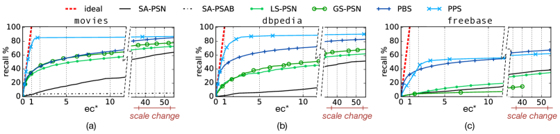
Figure 11: Recall progressiveness over the large, heterogeneous datasets.

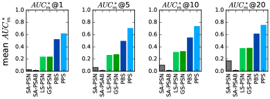
Figure 12: Mean $AUC_{m}^{*}$ over the large, heterogeneous datasets.

We now compare our schema-agnostic methods against the state-of-the-art schema-based method, i.e. PSN [4, 5], on the structured datasets. We assess the relative effectiveness of all methods with respect to recall progressiveness. The corresponding plots appear in Figure 9. They depict the performance of all methods for up to $ec^{*}{=}30$, i.e., we measure the recall for a number of comparisons thirty times the comparisons required by the ideal method to complete each ER task. We focus, though, on the interval [0,10] so as to highlight the behavior of the methods in the early stage of ER, the most critical for pay-as-you-go applications.

We observe that the advanced schema-agnostic methods outperform PSN, SA-PSN and SA-PSAB across all datasets. Only for census does PSN perform better than PBS (but not better that LS/GS-PSN) – see Figure 9a. This is because census contains very discriminative attributes, whose values are employed as blocking keys for PSN, identifying its duplicates with very high precision. Moreover, the profiles of census have short strings as attribute values: on average, every profile contains just 4-5 distinct tokens in its values. Inevitably, this sparse information has significant impact on the performance of similarity- and equality-based methods, restricting the co-occurrence patterns that lie at their core, i.e., the co-occurrences in windows for the former, and in blocks for the latter. The impact is larger in the latter case, due to the stricter definition of co-occurrence, which requires the equality of tokens, not just their similarity.

On the other hand, for datasets with high token overlap between matching profiles (i.e., they share many attribute value tokens) and non-discriminative attributes, which have the same value for many different profiles, our methods significantly outperform the schema-based PSN. For instance, the performance of PPS in the restaurant dataset (Figure 9b) is very close to the ideal method: $AUC_{PPS}^{*}@1$=0.93, i.e., 104 out of the first 112 emitted comparisons are matches.

Among the advanced methods, we now list the best performer for each dataset. On census (Figure 9a), GS-PSN is the best performer, but LS-PSN is only slightly worse. On restaurant (Figure 9b), PPS has the best progressiveness until recall 98%, but LS-PSN has a similar progressiveness and reaches 100% earlier than PPS (due to the plot scale, though, this is not evident in Figure 9). On cora (Figure 9c), GS-PSN has the best initial progressiveness, but equality-based methods reach the highest recall from $ec^{*}{=}4$ on—note that the final recall of PBS and PPS is lower than 100%, because the underlying Token Blocking cannot identify all duplicates in cora. On cddb (Figure 9d), PPS has the best progressiveness for recall up to 65%, but for higher recall, LS-PSN is the best performer.

We now compare all the methods with respect to their mean value of normalized area under the curve. Figure 10 shows the mean $AUC^{*}$ of all methods across all structured datasets for four different values of $ec^{*}$: 1, 5, 10 and 20. We observe that, on average, for any level of $AUC^{*}$, LS-PSN and GS-PSN are the top performers, in particular for the earliest phase of Progressive ER: their $AUC^{*}@1$ is three times the $AUC^{*}@1$ of PSN and PBS, and ${\sim}18\%$ higher than that of PPS.

Overall, we conclude that the best performing methods for structured datasets are LS-PSN and GS-PSN (the difference in their performance is insignificant. Thus, the selection of one method over the other should be driven by the differences in their space and time complexities for the initialization and emission phases, depending on $w_{max}$. The higher $w_{max}$ is, the higher gets the space complexity of GS-PSN in comparison to LS-PSN; thus, LS-PSN should be preferred when the availability of memory may be a issue. Yet, if memory is not an issue, GS-PSN should be preferred, as it avoids multiple emissions of the same comparisons.

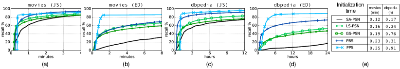
Figure 13: Time experiments with jaccard-sim (a,c) and edit-dist (b,d); initialization times (e).

7.2 Large, Heterogeneous Datasets

We now assess the relative performance of all methods with respect to recall progressiveness over the large, heterogeneous datasets movies, dbpedia, freebase. The corresponding plots appear in Figure 11.

The results confirm our intuition about the ineffectiveness of the naïve SA-PSN and SA-PSAB, since all advanced methods outperform it to a significant extent across all datasets. SA-PSAB also cannot scale to the largest datasets (see Figure 11b-c) due to the huge blocks in the highest layers of its suffix trees, which entail too many comparisons.

The only exceptions are LS-PSN and GS-PSN on freebase (Figure 11c), which perform poorly: the performance of LS-PSN is similar to that of SA-PSN, while GS-PSN has lower recall progressiveness than SA-PSN, terminating before achieving a recall greater that 20%. The performance of these two advanced methods can be explained by the characteristics of the dataset. Freebase is composed of RDF triples. The extracted tokens consist of RDF keywords, URI, and other RDF properties, which generate a noisy Neighbor List, since their alphabetical ordering is often meaningless. Thus, the RCF weighting scheme cannot approximate correctly the similarity of the profiles. On the other hand, PBS is able to get the most of the semantics in URI tokens, due to the equality requirement, thus being more robust on freebase than the similarity-based methods.

Overall, PPS is the best performer on movies (Figure 11a) and dbpedia (Figure 11b); while, on freebase (Figure 11c), PBS achieves the highest recall progressiveness for $ec^{*}{<}2$ and $ec^{*}{>}12$ (PPS is the best performer for $2{<}ec^{*}{<}12$). Again, to understand which method is the top performer, we compare them with respect to their mean value of normalized area under the curve. Figure 12 shows the mean $AUC_{m}^{*}$ of all methods across all datasets for four different values of $ec^{*}$: 1, 5, 10 and 20. We observe that PPS is the best performer for any level of $AUC_{m}^{*}$, and conclude that, overall, it is the best performing progressive method over large, heterogeneous datasets.

7.3 Time Efficiency Evaluation.

We note that our methods are general and decoupled from the match function employed to determine whether two profiles are matching or not. Yet, to assess their efficiency in terms of execution time, we evaluate them in combination with two match functions: edit distance (ED) [25] and Jaccard similarity (JS) [26]. The former is meant to test the performance of our methods with an expensive match function, while the latter with a cheap one. The time complexities of edit-distance and jaccard-sim are $O(s{\cdot}t)$ and $O(s{+}t)$, respectively, where $s$ and $t$ are the lengths of the two strings to be compared (i.e., the two profiles compared with the match function).

The schema-based methods are not considered in this evaluation, since they inherently require an additional overhead time to select the blocking keys (and to perform the schema-alignment in the case of Clean-clean ER). There is a plethora of techniques to perform these two tasks [27, 28, 29], but it is out of the scope of this work to determine which one is the best, since our proposed methods do not rely on them.

In Figure 13, we report the result of the time experiments on the datasets movies and dbpedia. (We do not consider freebase for this test, because Entity Matching for Linked Data typically requires more advanced, iterative algorithms like SiGMa [30]. In particular, Figures 13a-d plot the performance of all methods, considering both the initialization time and the comparison time. We did not plot the execution time for SA-PSAB because it is more than an order of magnitude slower than the other methods. The initialization times are listed in Figure 13e and are independent of the match function. Note that we do not report the emission time, as it is at least two orders of magnitude smaller than that required by the match functions to compare two profiles - this applies to all methods and datasets.

The results in Figure 13 clearly show that our advanced methods produce most of the matches much earlier than the baseline, in combination with both the expensive and the cheap match functions. Similarity- and equality-based methods show different performance characteristics, though. The difference in the initialization times between PBS/LS-PSN and the baseline is negligible for both match functions (see the left part of Figures 13a-d); hence, they are able to outperform the baseline since the early stages of the process. For PPS, the same consideration is valid only in case the expensive match function is employed (see the left part of Figures 13b,d). In fact, when the cheap match function is employed, its initialization time (55 minutes over DBPedia) may slightly affect the early stages of the process (Figures 13a,c);

8 Conclusions and Future Work

We have introduced schema-agnostic methods to maximize the recall progressiveness of Entity Resolution for pay-as-you-go applications, while addressing the Volume and Variety dimensions of Big Data. They can be distinguished into equality-based (PBS and PPS) and similarity-based methods (LS-PSN and GS-PSN). Our experimental evaluation with several real, structured datasets demonstrates that the proposed methods significantly outperform the schema-based state-of-the-art method in the field, PSN, identifying most of the matches much earlier.

Our experiments also indicate that both equality-based methods exhibit a quite robust performance across both structured and semi-structured (heterogeneous) datasets. In contrast, both similarity-based techniques achieve very high performance over structured datasets and very low over semi-structured datasets. The reason is the structured datasets are usually curated, principally containing character-level errors, whereas the semi-structured datasets abound in both character- and token-level noise (e.g., URIs as attribute values). In the latter cases, it is harder for two matching entities with similar attribute values to be placed in consecutive positions. We can conclude, therefore, that the similarity-based techniques can only be used over structured datasets, while the equality-based techniques perform well under all settings. In fact, PBS is suited for ER tasks involving cheap match functions and with very limited time budget (its initialization time is the lowest among the advanced methods). Otherwise, PPS achieves the best performance, both in terms of recall progressiveness (Figure 12) and execution time (Figure 13).

An interesting direction for extending our work is to examine the massive parallelization of our approach based on existing methods for parallelizing Sorted Neighborhood [31, 32] and Meta-blocking [33] in the context of MapReduce.

Giovanni Simonini is a postdoctoral researcher at the department of Engineering “Enzo Ferrari” of the University of Modena and Reggio Emilia, Italy. He received the PhD degree in Computer Science from the University of Modena and Reggio Emilia. His doctoral dissertation won the Best Thesis Award from the IEEE Computer Society Italy Section. His research focuses on data integration and big data management. George Papadakis is an internal auditor of information systems and a research fellow at the University of Athens. He has also worked at the NCSR ”Demokritos”, National Technical University of Athens (NTUA), L3S Research Center and ”Athena” Research Center. He holds a PhD in Computer Science from Hanover University and a Diploma in Computer Engineering from NTUA. His research focuses on web data mining. Themis Palpanas is Senior Member of the Institut Universitaire de France (IUF), and Professor of computer science at the Paris Descartes University (France), where he is the director of diNo, the data management group. He is the author of nine US patents, three of which have been implemented in world-leading commercial data management products. He is the recipient of three Best Paper awards, and the IBM Shared University Research (SUR) Award. He is serving as Editor in Chief for BDR Journal, Associate Editor for PVLDB 2019 and TKDE journal, and Editorial Advisory Board member for IS journal. Sonia Bergamaschi is full professor of Computer Engineering at the Engineering Department ”Enzo Ferrari” of the University of Modena and Reggio Emilia, where she is leading the database research group ”DBGroup”. Her research activity has been mainly devoted to knowledge representation and management in the context of very large databases. She was coordinator and participant of many ICT European projects. She has published more than two hundred international journal and conference papers. She has served on the committees of the main international Database and AI conferences. She is an ACM Distinguished Scientist and an IEEE senior Member.

References

- [1] V. Christophides, V. Efthymiou, and K. Stefanidis, Entity Resolution in the Web of Data. Morgan & Claypool, 2015.
- [2] X. L. Dong and D. Srivastava, Big Data Integration. Morgan & Claypool, 2015.
- [3] L. Getoor and A. Machanavajjhala, “Entity resolution: Theory, practice & open challenges,” PVLDB, vol. 5, no. 12, pp. 2018–2019, 2012.
- [4] T. Papenbrock, A. Heise, and F. Naumann, “Progressive duplicate detection,” IEEE TKDE, vol. 27, no. 5, pp. 1316–1329, 2015.
- [5] S. E. Whang, D. Marmaros, and H. Garcia-Molina, “Pay-as-you-go entity resolution,” IEEE TKDE, vol. 25, no. 5, pp. 1111–1124, 2013.
- [6] B. Golshan, A. Y. Halevy, G. A. Mihaila, and W. Tan, “Data integration: After the teenage years,” in PODS, 2017, pp. 101–106.
- [7] G. Papadakis, G. Alexiou, G. Papastefanatos, and G. Koutrika, “Schema-agnostic vs schema-based configurations for blocking methods on homogeneous data,” PVLDB, vol. 9, no. 4, pp. 312–323, 2015.
- [8] M. A. Hernández and S. J. Stolfo, “The merge/purge problem for large databases,” in SIGMOD, 1995, pp. 127–138.
- [9] Y. Altowim and S. Mehrotra, “Parallel progressive approach to entity resolution using mapreduce,” in ICDE, 2017, pp. 909–920.
- [10] Y. Altowim, D. V. Kalashnikov, and S. Mehrotra, “Progressive approach to relational entity resolution,” PVLDB, vol. 7, no. 11, 2014.
- [11] S. E. Whang and H. Garcia-Molina, “Joint entity resolution,” in ICDE, 2012, pp. 294–305.
- [12] G. Papadakis, G. Papastefanatos, T. Palpanas, and M. Koubarakis, “Scaling entity resolution to large, heterogeneous data with enhanced meta-blocking,” in EDBT, 2016, pp. 221–232.
- [13] J. Wang, T. Kraska, M. J. Franklin, and J. Feng, “Crowder: Crowdsourcing entity resolution,” PVLDB, vol. 5, no. 11, pp. 1483–1494, 2012.
- [14] N. Vesdapunt, K. Bellare, and N. N. Dalvi, “Crowdsourcing algorithms for entity resolution,” PVLDB, vol. 7, no. 12, pp. 1071–1082, 2014.
- [15] J. Wang, G. Li, T. Kraska, M. J. Franklin, and J. Feng, “Leveraging transitive relations for crowdsourced joins,” in SIGMOD, 2013.
- [16] D. Firmani, B. Saha, and D. Srivastava, “Online entity resolution using an oracle,” PVLDB, vol. 9, no. 5, pp. 384–395, 2016.
- [17] O. Benjelloun, H. Garcia-Molina, D. Menestrina, Q. Su, S. E. Whang, and J. Widom, “Swoosh: a generic approach to entity resolution,” VLDB J., vol. 18, no. 1, pp. 255–276, 2009.
- [18] G. Papadakis, E. Ioannou, C. Niederée, and P. Fankhauser, “Efficient entity resolution for large heterogeneous information spaces,” in WSDM, 2011, pp. 535–544.
- [19] P. Christen, “A survey of indexing techniques for scalable record linkage and deduplication,” IEEE TKDE, vol. 24, no. 9, pp. 1537–1555, 2012.
- [20] G. Simonini, S. Bergamaschi, and H. V. Jagadish, “BLAST: a loosely schema-aware meta-blocking approach for entity resolution,” PVLDB, vol. 9, no. 12, pp. 1173–1184, 2016.
- [21] A. Aizawa and K. Oyama, “A fast linkage detection scheme for multi-source information integration,” in WIRI, 2005.
- [22] H. Köpcke, A. Thor, and E. Rahm, “Evaluation of entity resolution approaches on real-world match problems,” PVLDB, vol. 3, no. 1, pp. 484–493, 2010.
- [23] A. Harth, “Billion Triples Challenge data set,” Downloaded from http://km.aifb.kit.edu/projects/btc-2009/, 2009.
- [24] D. Song, Y. Luo, and J. Heflin, “Linking heterogeneous data in the semantic web using scalable and domain-independent candidate selection,” IEEE TKDE., vol. 29, no. 1, pp. 143–156, 2017.
- [25] G. Bard, “Spelling-error tolerant, order-independent pass-phrases via the damerau-levenshtein string-edit distance metric,” in ACSW Frontiers 2007, 2007, pp. 117–124.
- [26] J. Leskovec, A. Rajaraman, and J. D. Ullman, Mining of Massive Datasets, 2nd Ed. Cambridge University Press, 2014.
- [27] S. Melnik, H. Garcia-Molina, and E. Rahm, “Similarity flooding: A versatile graph matching algorithm and its application to schema matching,” in ICDE, 2002, pp. 117–128.
- [28] P. Shvaiko and J. Euzenat, “Ontology matching: State of the art and future challenges,” IEEE TKDE, vol. 25, no. 1, pp. 158–176, 2013.
- [29] M. Michelson and C. A. Knoblock, “Learning blocking schemes for record linkage,” in AAAI, pp. 440–445.
- [30] S. Lacoste-Julien, K. Palla, A. Davies, G. Kasneci, T. Graepel, and Z. Ghahramani, “Sigma: simple greedy matching for aligning large knowledge bases,” in KDD, 2013, pp. 572–580.
- [31] K. Ma, F. Dong, and B. Yang, “Large-scale schema-free data deduplication approach with adaptive sliding window using mapreduce,” Comput. J., vol. 58, no. 11, pp. 3187–3201, 2015.
- [32] D. G. Mestre, C. E. S. Pires, and D. C. Nascimento, “Adaptive sorted neighborhood blocking for entity matching with mapreduce,” in ACM SIGAPP, 2015, pp. 981–987.
- [33] V. Efthymiou, G. Papadakis, G. Papastefanatos, K. Stefanidis, and T. Palpanas, “Parallel meta-blocking for scaling entity resolution over big heterogeneous data,” Inf. Syst., vol. 65, pp. 137–157, 2017.