Evidence for a circumplanetary disk around protoplanet PDS 70 b

Abstract

We present the first observational evidence for a circumplanetary disk around the protoplanet PDS 70 b, based on a new spectrum in the $K$ band acquired with VLT/SINFONI. We tested three hypotheses to explain the spectrum: Atmospheric emission from the planet with either (1) a single value of extinction or (2) variable extinction, and (3) a combined atmospheric and circumplanetary disk model. Goodness-of-fit indicators favour the third option, suggesting circumplanetary material contributing excess thermal emission — most prominent at $\lambda\gtrsim 2.3\mu$m. Inferred accretion rates ($\sim 10^{-7.8}$–$10^{-7.3}M_{J}$ yr^-1) are compatible with observational constraints based on the H$\alpha$ and Br$\gamma$ lines. For the planet, we derive an effective temperature of 1500–1600 K, surface gravity $\log(g)\sim 4.0$, radius $\sim 1.6R_{J}$, mass $\sim 10M_{J}$, and possible thick clouds. Models with variable extinction lead to slightly worse fits. However, the amplitude ($\Delta A_{V}\gtrsim 3$mag) and timescale of variation ($\lesssim$ years) required for the extinction would also suggest circumplanetary material.

1 Introduction

Discovery of the Galilean moons of Jupiter (Galilei, 1610) led to the overthrow of Geocentric cosmology, and Galileo’s subsequent denouncement, trial and house arrest. Their hypothesised origin is a circumplanetary disk (CPD) of gas and dust (e.g. Lunine & Stevenson, 1982; Lissauer, 1993). Analytic work (Pollack et al., 1979; Canup & Ward, 2002; Papaloizou & Nelson, 2005) and increasingly sophisticated numerical simulations (e.g. Lubow et al., 1999; Ayliffe & Bate, 2009; Gressel et al., 2013; Szulágyi et al., 2017) have consolidated this hypothesis.

Observational evidence has so far remained elusive. Searches using mm-continuum have produced only non-detections (e.g. Isella et al., 2014; Wu et al., 2017; Wolff et al., 2017). High-contrast infrared (IR) observations have been suggested instead to capture the thermal excess from the CPD (e.g. Zhu, 2015; Eisner, 2015; Montesinos et al., 2015). The power of high-contrast IR spectroscopy to characterize young substellar companions has been demonstrated over the last few years (e.g. Allers & Liu, 2013; Bonnefoy et al., 2014; Delorme et al., 2017). Observed spectra are fitted to either synthetic atmospheric models or observed template spectra which enable the estimation of effective temperature, surface gravity and radius of the planet, which can then be used to estimate its mass and age. Constraints on clouds or haze in the atmosphere can also be obtained (e.g. Madhusudhan et al. 2011, hereafter M11; see Madhusudhan (2019) for a recent review).

We present evidence for a circumplanetary disk around the recently discovered protoplanet PDS 70 b. PDS 70 is a young K7-type star surrounded by a pre-transitional disk with a large annular gap (Hashimoto et al., 2012; Dong et al., 2012). The protoplanet was first detected in this gap using VLT/SPHERE (Keppler et al., 2018; Müller et al., 2018, hereafter M18). Subsequent search for sub-mm emission from a CPD using ALMA was inconclusive (Keppler et al., 2019). Spectral characterisation of the planet was presented in M18, suggesting an effective temperature of $\sim$1000-1500 K, surface gravity $\lesssim 3.5$dex and mass $\leq 17M_{\rm J}$. We present a new spectral characterization of PDS 70 b, including both the measurements presented in M18 and a new spectrum in $K$ band obtained with VLT/SINFONI (Christiaens et al., 2019, hereafter C19). The spectrum shows excess emission at $\lambda\gtrsim 2.3\mu$m inconsistent with naked model atmospheres of young planets, indicating the presence of circumplanetary material.

2 Observations

M18 presented a $YJH$ spectrum and multi-epoch broadband photometric measurements, acquired with SPHERE/IFS ($YJH$), SPHERE/IRDIS ($H1$/$H2$ and $K1$/$K2$), NICI ($L^{\prime}$) and NACO ($L^{\prime}$). We gathered all measurements quoted in M18, but considered updated values for their $L^{\prime}$-band flux estimates. M18 fitted the SED of the star to estimate its $L^{\prime}$ flux, without including possible excess disk emission. That value was then multiplied by the contrast of the companion to infer its flux. However, most of excess IR emission compared to the star likely arises from hot dust in the inner disk that would be unresolved from the star at $L^{\prime}$ band, and should hence be included. By contrast, the contribution from resolved scattered light from the disk at $L^{\prime}$ band is negligible (see images in Keppler et al., 2018). Given the importance of the thermal IR flux to the hypothesis of a CPD around PDS 70 b, we re-estimated the $L^{\prime}$ flux of the companion considering (1) the $L^{\prime}$ flux of the star + unresolved inner disk by interpolating the photometric measurements in the W1 ($3.35\mu$m) and W2 ($4.60\mu$m) filters of WISE (Wright et al., 2010), and (2) the same values for the contrast of the companion as in M18. The new $L^{\prime}$ estimates of the companion are: $(8.55\pm 3.38)\times 10^{-17}$ W m^-2 $\mu$m^-1 and $(6.70\pm 4.05)\times 10^{-17}$ W m${}^{-2}\mu$m for the NICI and NACO data, respectively.

In a recent paper (C19), we inferred the contrast of the protoplanet with respect to the star as a function of wavelength, $c(\lambda)$, in the $K$ band at unprecedented spectral resolution ($R\sim 100$ after spectral binning) using VLT/SINFONI. We employed two different methods for extracting $c(\lambda)$, both leading to flux estimates consistent with each other at all wavelengths. Here, we consider only the spectrum inferred with ANDROMEDA (Cantalloube et al., 2015, Cantalloube et al. 2019 in prep.) since it has smaller uncertainties and higher spectral resolution, and avoids the risk of contamination by extended (resolved) disk signals.

Despite the higher quality of the ANDROMEDA $c(\lambda)$, some spectral channels contain outliers. In order to minimize the risk of bias, we first removed spectral channels with a detection below 3$\sigma$ and lying in strong telluric lines, then used a Savitzky-Golay filter of order 3 with a 81-channel window to smooth the $c(\lambda)$ curve before binning it by a factor of 20 (Savitzky & Golay, 1964). We obtained the final $K$-band spectrum of the protoplanet by multiplying $c(\lambda)$ with the calibrated spectrum of the star measured with the SpeX spectrograph (Long et al., 2018), after resampling the latter at the spectral resolution of the binned SINFONI spectral channels.

In total, our SED has 86 data points; 49 from M18 and 37 obtained with SINFONI (C19). Measurements span 6 years, extending from 2012/03 to 2018/02. Flux estimates at overlapping wavelengths are all consistent with each other except one. Namely, our SINFONI flux estimates (2014/05 epoch) are slightly higher than the 2018/02 epoch SPHERE measurement in the $K2$ filter (2.25$\mu$m).

3 Spectral analysis

We first attempted to fit the observed SED with synthetic spectra modeling pure atmospheric emission (Section 3.1). We considered a single value of extinction for all epochs, treated as a free parameter in the spectral fit (referred to as Type I models hereafter). Given the discrepancy between the SPHERE $K2$ and SINFONI $K$-band measurements, we also considered a fit with variable amount of extinction for different epochs (Type II models). Finally, we also examined models consisting of combined emission from an atmosphere and a circumplanetary disk with a variable accretion rate (Type III models; Section 3.2). In order to minimise the number of free parameters, we considered only two possible values of extinction (for Type II models) and two accretion rates (for Type III models); one value for the SINFONI (2014/05), SPHERE (2016/05) and NICI (2012/03) epochs, and the other for all other epochs. This division was chosen because (1) the SPHERE IFS ($YJH$)+IRDIS ($K1$/$K2$) were obtained simultaneously on 2018/02, and the IRDIS $H1$/$H2$ points of 2015/05 are consistent with the IFS spectrum, and (2) the SINFONI 2014/05 data are brighter than the IRDIS $K2$ point of 2018/02, while the IRDIS $K2$ point of 2016/05 is in better agreement with the SINFONI data. For the NICI and NACO points, we arbitrarily assigned them to the first and second group, respectively.

For all model types, we minimised the following goodness-of-fit indicator:

$$\chi^{2}=\sum_{i}\omega_{i}\big{[}\frac{F_{\rm obs}(\lambda_{i})-F_{\rm model}(\lambda_{i})}{\sigma_{i}}\big{]}^{2}$$ (1)

where $\sigma_{i}$ is the uncertainty in the flux measurement $F_{\rm obs}(\lambda_{i})$ at wavelength $\lambda_{i}$, and weights $\omega_{i}$ are defined for photometric and spectroscopic observations following a similar strategy as in Ballering et al. (2013) and Olofsson et al. (2016). Weights are proportional to the FWHM of the filters used (for broadband photometric measurements), or the spectral resolution (for SPHERE/IFS and SINFONI data). The sum of all weights is normalized to the total number of points. We define a reduced goodness-of-fit indicator $\chi_{r}^{2}$ as $\chi^{2}$ divided by the respective number of degrees of freedom for each type of model.

3.1 Atmospheric models

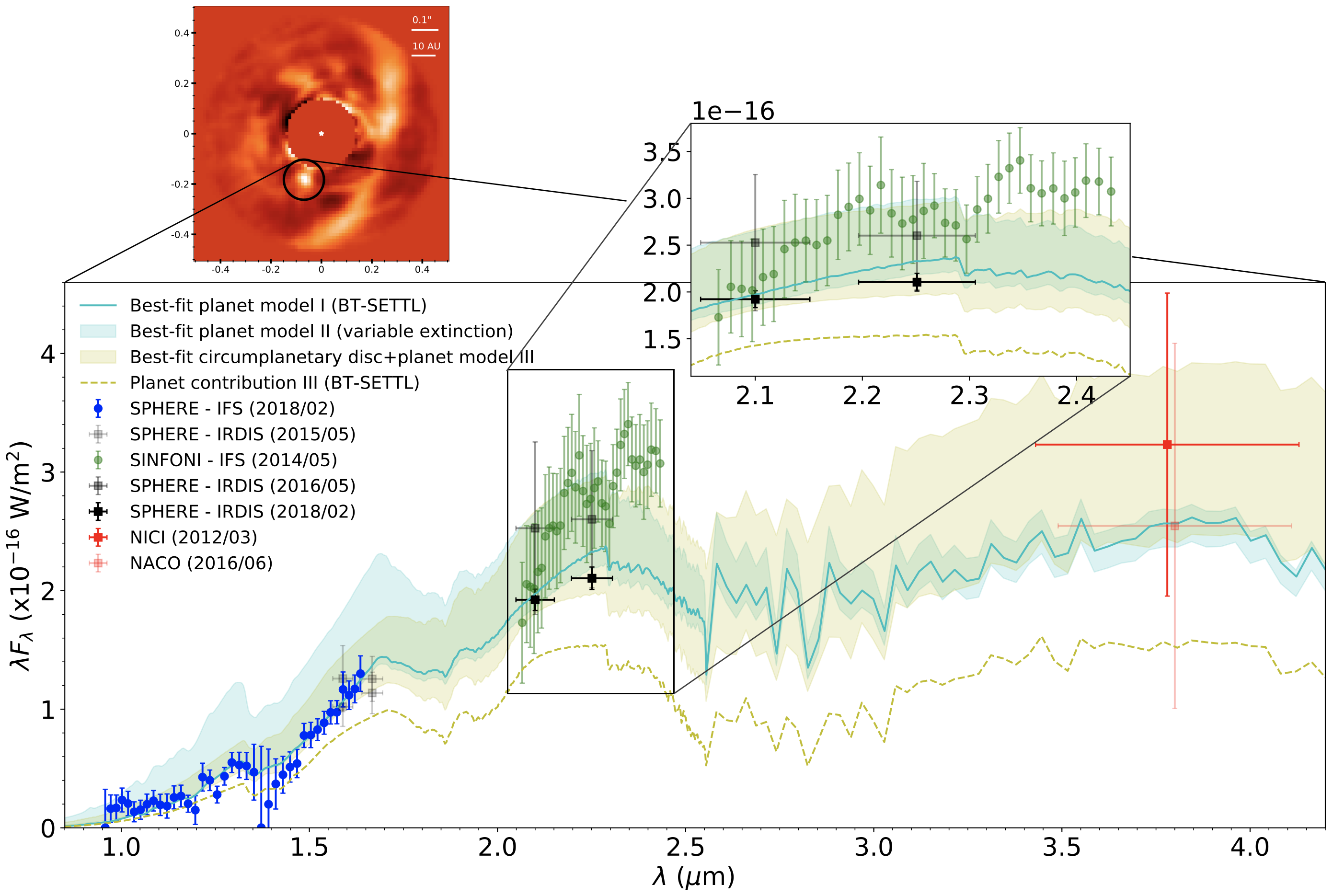
Figure 1: Combined spectrum of PDS 70 b compared to best-fit BT-SETTL models consisting of pure atmospheric emission without (solid cyan line) or with variable extinction (shaded blue area). Shaded yellow area shows best-fit atmosphere+CPD model. Circles with vertical error bars are IFS measurements, while squares with vertical and horizontal error bars are broad-band measurements. Inset highlights new SINFONI spectrum (green points). The SINFONI spectrum shows a $\sim 2\sigma$ IR excess at $\lambda>2.3\mu$m compared to best-fit atmospheric models, best accounted for by the presence of a CPD. Top image shows image of PDS 70 b with SINFONI (from C19, ).

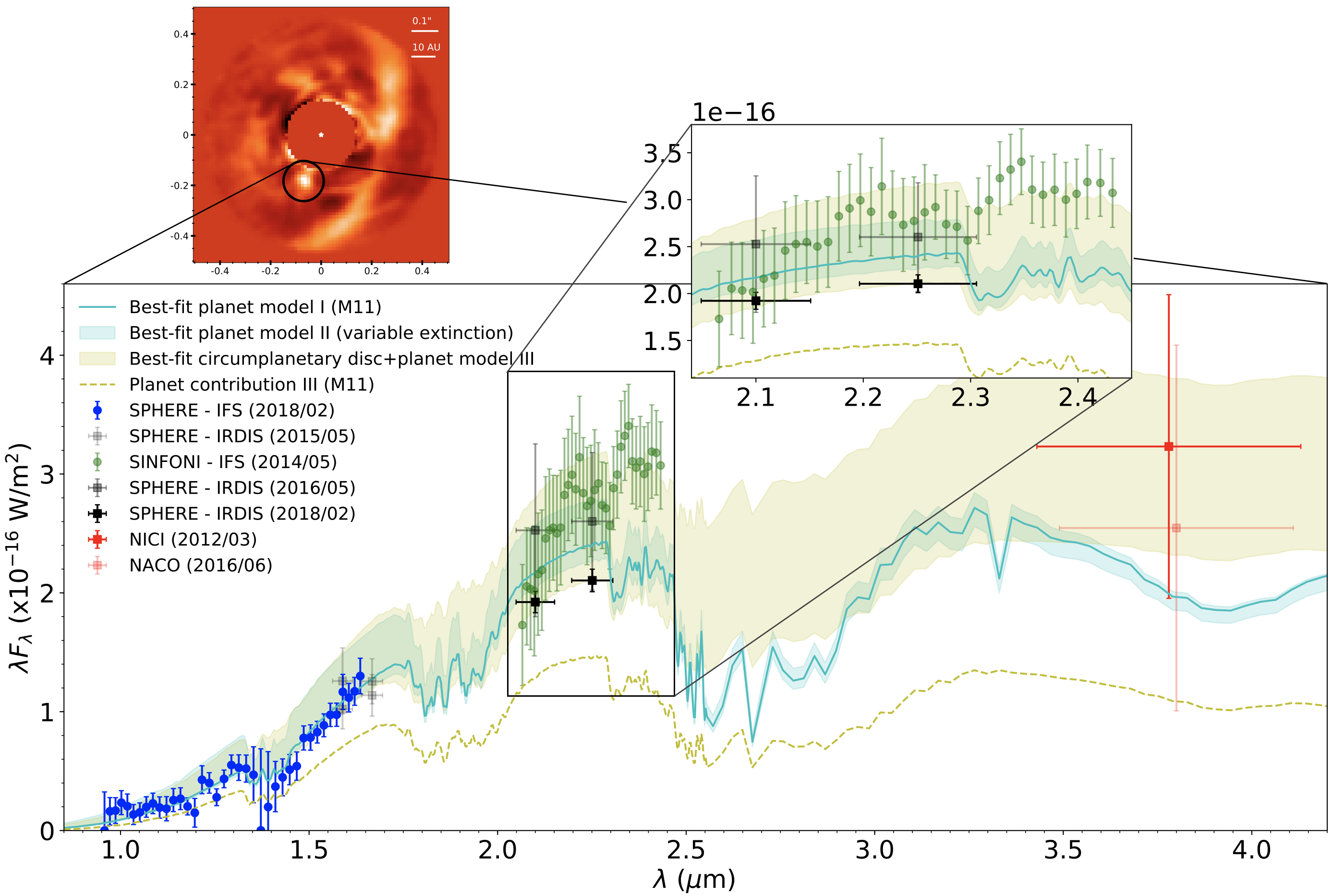
Figure 2: Same as Figure 1 but using M11 models. Again, the best fit is obtained with a circumplanetary disc.

We considered two grids of synthetic spectra: BT-SETTL models (Allard et al., 2012; Baraffe et al., 2015), and the grid of atmospheric models presented in M11. These models treat dust and clouds differently. BT-SETTL models account for dust formation using a parameter-free cloud model. They consider cloud microphysics — the particle size of each species is calculated self-consistently based on condensation and sedimentation mixing timescales. Free parameters are the effective temperature, varied between 1200 and 1900 K (steps of 100 K), and the surface gravity, $\log(g)$, explored between 3.0 and 5.0 (steps of 0.5 dex). We assumed Solar metallicity.

M11 considered a wide grid of cloud models, with different geometrical and optical thickness, particle size and metallicities. The M11 models do not include microphysics. They consider different cloud spatial structure and particle sizes; labeled A, AE, AEE or E, based on the rapidity with which clouds are cut off at their upper end. Several modal particle sizes are considered, including 1, 60 and 100 $\mu$m. The grid also includes cloud-free models (NC), with both equilibrium and non-equilibrium chemistry. In the latter case, two additional free parameters arise: the eddy diffusion coefficient $K_{zz}$ taking possible values of $10^{2}$, $10^{4}$ or $10^{6}$ cm² s^-1, and the sedimentation parameter $f_{\rm sed}$ (defined as in Ackerman & Marley, 2001). M11 varied these parameters on a grid of effective temperature and surface gravity ranging from 600 to 1800 K (steps of 100 K) and from 3.5 to 5.0 (steps of 0.5 dex), respectively.

For both BT-SETTL and M11 models, we treated the planet radius as a free parameter to scale the total emergent flux. We explored values between 0.1 and 5.0 $R_{\rm J}$ in steps of 0.1 $R_{\rm J}$. We also considered dust extinction as an additional free parameter, with allowed values between $A_{V}=0$ and $10.0$ mag (steps of 0.2 mag). For Type II models, we explored both minimum and maximum extinction values within this grid. We considered the extinction curve for interstellar dust (Draine, 1989). Considering other dust species (e.g. typical species found in the atmosphere of brown dwarfs) would increase the number of free parameters, and is not expected to give qualitatively different slopes after dereddening (see e.g. Marocco et al., 2014). We assumed a distance of 113 pc (Gaia Collaboration et al., 2018).

Table 1: Best fit parameters for PDS 70 b

I. Planet alone			II. Planet alone (variable extinction)			III. Planet and circumplanetary disc
Parameter	Range	Best fit	Parameter	Range	Best fit	Parameter	Range	Best fit
BT-SETTL atmospheric models
$T_{\mathrm{eff}}$ [K]	1200–1900	1500	$T_{\mathrm{eff}}$ [K]	1200–1900	1500	$T_{\mathrm{eff}}$ [K]	1200–1900	1500
$\log(g)$	3.0–5.0	3.0	$\log(g)$	3.0–5.0	3.0	$\log(g)$	3.0–5.0	4.0
$R_{\rm b}$ [$R_{\rm J}$]	0.1–5.0	2.2	$R_{\rm b}$ [$R_{\rm J}$]	0.1–5.0	2.1	$R_{\rm b}$ [$R_{\rm J}$]	0.1–2.0	1.6
$A_{V}$ [mag]	0.0–10.0	4.34	$A_{V\mathrm{,1}}$ [mag]	0.0–10.0	0.60	$A_{V}$ [mag]	0.0–10.0	6.40
			$A_{V\mathrm{,2}}$ [mag]	0.0–10.0	4.00	$M_{\rm b}\dot{M}_{\rm b,1}$ [$M_{\rm J}^{2}$yr-1]	$10^{-7}$–$10^{-6}$	$10^{-6.4}$
						$M_{\rm b}\dot{M}_{\rm b,2}$ [$M_{\rm J}^{2}$yr-1]	$10^{-7}$–$10^{-6}$	$10^{-6.8}$
$M_{\rm b}^{\dagger}$ [$M_{\rm J}$]	–	1.9	$M_{\rm b}^{\dagger}$ [$M_{\rm J}$]	–	1.7	$M_{\rm b}^{\dagger}$ [$M_{\rm J}$]	–	9.9
						$\dot{M}_{\rm b}^{\dagger}$ [$M_{\rm J}$yr-1]	–	$10^{-7.8}$–$10^{-7.4}$
		$\chi_{r}^{2}\sim 1.01$			$\chi_{r}^{2}\sim 0.52$			$\chi_{r}^{2}\sim 0.41$
M11 atmospheric models
$T_{\mathrm{eff}}$ [K]	600–1800	1100	$T_{\mathrm{eff}}$ [K]	600–1800	1200	$T_{\mathrm{eff}}$ [K]	600–1800	1600
$\log(g)$	3.5–5.5	4.0	$\log(g)$	3.5–5.5	4.0	$\log(g)$	3.5–5.5	4.0
$R_{\rm b}$ [$R_{\rm J}$]	0.1–5.0	3.3	$R_{\rm b}$ [$R_{\rm J}$]	0.1–5.0	2.8	$R_{\rm b}$ [$R_{\rm J}$]	0.1–2.0	1.6
$c$	[NC,E,A,…]‡	A	$c$	[NC,E,A,…]‡	A	$c$	[NC,E,A,…]‡	A60‡
$f_{\rm sed}$	[eq.,0,1,2]	eq.	$f_{\rm sed}$	[eq.,0,1,2]	eq.	$f_{\rm sed}$	[eq.,0,1,2]	eq.
$K$ [cm2s-1]	[eq.,$10^{2}$–$10^{6}$]	eq.	$K$ [cm2s-1]	[eq.,$10^{2}$–$10^{6}$]	eq.	$K$ [cm2s-1]	[eq.,$10^{2}$–$10^{6}$]	eq.
$A_{V}$ [mag]	0.0–10.0	3.00	$A_{V\mathrm{,1}}$ [mag]	0.0–10.0	0.80	$A_{V}$ [mag]	0.0–10.0	8.72
			$A_{V\mathrm{,2}}$ [mag]	0.0–1.2	4.00	$M_{\rm b}\dot{M}_{\rm b,1}$ [$M_{\rm J}^{2}$yr-1]	$10^{-7}$–$10^{-6}$	$10^{-6.3}$
						$M_{\rm b}\dot{M}_{\rm b,2}$ [$M_{\rm J}^{2}$yr-1]	$10^{-7}$–$10^{-6}$	$10^{-6.7}$
$M_{\rm b}^{\dagger}$ [$M_{\rm J}$]	–	42.0	$M_{\rm b}^{\dagger}$ [$M_{\rm J}$]	–	30.2	$M_{\rm b}^{\dagger}$ [$M_{\rm J}$]	–	9.9
						$\dot{M}_{\rm b}^{\dagger}$ [$M_{\rm J}$yr-1]	–	$10^{-7.7}$–$10^{-7.3}$
		$\chi_{r}^{2}\sim 1.20$			$\chi_{r}^{2}\sim 0.70$			$\chi_{r}^{2}\sim 0.44$
† $M_{\rm b}$ is inferred from the best-fit $\log(g)$ and $R_{\rm b}$ values, and $\dot{M}_{\rm b}$ is inferred from $M_{\rm b}$ and the best-fit $M_{\rm b}\dot{M}_{\rm b}$.
‡ See Section 3.1 and M11. A60 refers to model cloud A (thickest) with a modal particle size of 60 $\mu$m.

Figures 1 and 2 compare our best-fit models from the BT-SETTL and M11 grids, respectively, with the SED of PDS 70 b. Table 1 gives the explored parameter ranges, best-fit parameter values and corresponding $\chi_{r}^{2}$, for each model. Best-fit Type I BT-SETTL and M11 models reproduce most of the observed SED but are a poor match to the red end of the SINFONI spectrum, with a $>2\sigma$ discrepancy for most data points at wavelengths $\gtrsim 2.3\mu$m. They lead to reduced goodness-of-fit indicators $\chi_{r}^{2}\sim 1.01$ and 1.20.

Allowing for variable extinction (Type II) yields best-fit models (shaded cyan areas in Figures 1 and 2) in better agreement with flux estimates longward of $\sim 2.3\mu$m ($\chi_{r}^{2}\sim 0.52$ and 0.70). Upper and lower edges of the shaded areas correspond to the minimum and maximum extinction values ($A_{V,1}$ and $A_{V,2}$, in Table 1) of our best-fit model, with $A_{V,1}$ better accounting for the 2014/05 SINFONI, 2016/05 SPHERE and 2012/03 NICI data points and $A_{V,2}$ accounting for data points at all other epochs. The difference in extinction is $A_{V}\gtrsim 3$ mag for both BT-SETTL and M11 models.

For both Type I and II models, the best-fit effective temperatures (1100–1500 K), surface gravity ($\log(g)\sim 3.0$–$4.0$), planet radius ($2.1$–$3.3R_{J}$) and hence mass (1.7–42.0 $M_{J}$) are in approximate agreement with the previous estimates made in M18. Our mass estimates are uncertain because of the large steps in $\log(g)$ (0.5 dex) in our model grids, and hence do not rule out a brown dwarf. Our best-fit M11 models correspond to the thickest cloud models (labelled A); extending to the top of the atmosphere.

3.2 Combined atmospheric+CPD models

For our Type III models (combined atmosphere+CPD emission), we considered the same two grids of atmospheric models as in Section 3.1, coupled with the CPD models presented in Eisner (2015). The latter add a single free parameter, the mass accretion rate, which sets the brightness and shape of the CPD spectrum. We explored values of mass accretion rates $\log(\dot{M}_{b}M_{b}[M_{J}^{2}\textrm{yr}^{-1}])$ ranging from -7.0 to -6.0, in steps of 0.1 dex. We did not consider accretion rates smaller than $10^{-7}M_{J}^{2}$ yr^-1 because the corresponding models do not contribute significantly at NIR wavelengths. We assume a fixed inner truncation radius of $2R_{\rm J}$ in our CPD models, as in Eisner (2015). We thus truncated our grid of planetary radii to $2R_{\rm J}$ for consistency. Other parameters were explored on the same grids as for Type I and II models.

Figures 1 and 2 show the best-fit combined planet+CPD models (shaded yellow areas). Dashed lines show the contribution from the atmosphere alone. Upper and lower edges of the shaded areas correspond to maximum and minimum mass accretion rates of our best fit model ($M_{b}\dot{M}_{b,1}$ and $M_{b}\dot{M}_{b,2}$, respectively, in Table 1), accounting for the 2014/05 SINFONI and 2016/05 SPHERE data points and, respectively, data points at all other epochs. The planet+CPD best-fit models reproduce better the observed spectrum than pure atmospheric models (with or without variable accretion), with reduced goodness-of-fit indicators $\chi_{r}^{2}\sim 0.41$ and 0.44 using BT-SETTL and M11 models, respectively. Interestingly, the best-fit parameters for both the CPD and the planet are similar using either BT-SETTL or M11 models: mass accretion rates ranging between $\sim 10^{-6.4}$ and $\sim 10^{-6.8}$ $M_{J}^{2}$ yr^-1, effective temperature of 1500–1600 K, surface gravity $\log(g)\sim 4.0$, radius of $\sim 1.6R_{J}$, and mass of $\sim 10M_{J}$. The M11 best-fit model also suggests the thickest cloud geometry, with a modal particle size of 60 $\mu$m.

The estimate of 10 $M_{J}$ is larger than that inferred from the planet-only BT-SETTL models because the estimated $\log(g)$ is significantly larger, while the inferred $R_{b}$ is slightly smaller. For M11 models the opposite is true because $\log(g)$ is similar but $R_{b}$ is smaller. This suggests an older planet when considering a CPD in the model. Interestingly, the estimated planet parameters ($T_{\rm eff}$, $\log(g)$, $R_{b}$, $M_{b}$) agree with the BT-SETTL models for a mass of $10M_{J}$ and age 9–11 Myr (Baraffe et al., 2015). The inferred age is consistent with estimates for the star in Pecaut & Mamajek (2016), but not with the newer estimate of $5.4\pm 1.0$ Myr (M18). In contrast, parameters in planet-only models are inconsistent with Baraffe et al. (2015) evolutionary models for any combination of mass and age.

4 Discussion

We explored the hypothesis of variability for PDS 70 b because of the absence of atmospheric models red enough to account for both the 2018/02 SPHERE $K2$ measurement and the points at $\gtrsim 2.3\mu$m in our 2014/05 SINFONI spectrum. This is further supported by the disagreement (albeit slight) between the SPHERE and SINFONI measurements at $\sim 2.25\mu$m. Since the variability of classical T-Tauri stars is thought to be related to either variable amounts of extinction from intervening circumstellar dust (e.g. Bozhinova et al., 2016) or irregular accretion (e.g. Bouvier et al., 2004; Rigon et al., 2017), we tested similar hypotheses in our type II and III models, respectively. Accretion variability has also been predicted in magnetohydrodynamics simulations of forming planets (e.g. Gressel et al., 2013), further justifying type III models.

The best fit to the SED of PDS 70 b is obtained with an atmosphere+CPD model. Nonetheless, our caveats are:

1. We considered a limited range of atmospheric models. Atmospheric models have been proposed in recent years with different levels of complexity, including for example microphysics, non-equilibrium chemistry, or clouds/hazes (see Madhusudhan, 2019, and references therein). We used the two most complete publicly available synthetic atmospheric model grids, which successfully reproduce the spectrum of adolescent giant exoplanets such as Beta Pic b or HR 8799 b, c, d and e (M11; Bonnefoy et al., 2013; Currie et al., 2014). Given that our best-fit type I (purely atmospheric) BT-SETTL and M11 models are similar to the reddest atmospheric models (around $\sim 2.3\mu$m) presented in M18, we do not expect our conclusion of an excess at $\gtrsim 2.3\mu$m to change using different grids of atmospheric models.

2. The fit is not perfect. Although the best-fit atmosphere+CPD model best reproduces the excess at the end of the $K$ band, it does not perfectly reproduce the observed slope around 2.3$\mu$m. For both the BT-SETTL and M11 type III models, most photometric points at wavelengths shorter than 2.3 $\mu$m lie below the model (albeit all within 2$\sigma$), while most points longward of 2.3 $\mu$m are slightly brighter than the model (but within 2$\sigma$ also).

3. The assumptions behind our CPD models may be incorrect. Incorrect assumptions may explain why our CPD models do not reproduce perfectly the observed steep slope. We fixed the inner truncation radius to 2$R_{J}$. As shown in Zhu (2015), different inner truncation radii can lead to different predicted CPD spectra for a given mass accretion rate. Furthermore, neither the models in Zhu (2015) nor in Eisner (2015) take into account radiative feedback from the protoplanet itself. The best-fit effective temperature and radius found for PDS 70 b suggest a protoplanet luminosity $L_{p}\sim 10^{-4}L_{\odot}$. Montesinos et al. (2015) showed that the effect of such bright protoplanet would be to further increase the IR excess of the CPD with a steeper spectral slope, hence possibly improving the match with the K-band spectrum of PDS 70 b. New dedicated simulations are required to verify this hypothesis.

However, several lines of evidence support the hypothesis of circumplanetary material:

1. Our best-fit accretion rates agree with observations. Assuming a similar relationship between H$\alpha$ luminosity and mass accretion rate as T-Tauri stars, Wagner et al. (2018) estimated the PDS 70 b accretion rate as $\sim 10^{-7.8}M_{\rm J}^{2}R_{\rm J}^{-1}$ yr^-1 in the absence of extinction. However, the protoplanet is likely to be embedded within the circumplanetary material from which it feeds. The observed accretion rate would then be $\sim 10^{-6.7}M_{\rm J}^{2}R_{\rm J}^{-1}$ yr^-1 for $A_{V}\approx 3$mag. Assuming a similar relationship for Br$\gamma$ emission, C19 also constrained the accretion rate to be $<10^{-6.2}M_{\rm J}^{2}R_{\rm J}^{-1}$ yr^-1, considering negligible extinction at $K$ band. Our best-fit models suggest strong extinction towards the protoplanet ($A_{V}>6$mag), consistent with the presence of a CPD. Our estimates of mass ($M_{b}\sim 10M_{J}$), accretion rates ($\sim 10^{-7.5}M_{J}$ yr^-1), extinction ($\gtrsim 6$ mag) and radii $R_{\rm b}$ ($\sim 1.6R_{J}$), appear roughly compatible with both observational constraints. Monitoring of the H$\alpha$ luminosity would confirm the variability of the accretion rate.

2. The photometric variability is only observed at relatively long NIR wavelength ($\sim 2.2\mu$m). The best-fit models involving variable extinction lead to only slightly worse fits to the data than the atmosphere+CPD best-fit models. However, for the former models the amplitude of the variability is larger at short than at long NIR wavelengths, which is not observed despite multiple epoch observations at wavelengths shorter than 1.7 $\mu$m. Even if the variability was due to extinction, given the radial separation of the protoplanet ($\sim 20$au), both the amplitude ($\Delta A_{V}\gtrsim 3$ mag) and timescale of extinction variability (less than several years) suggests it would also be caused by circumplanetary dust.

3. Tentative excess with respect to the atmosphere+CPD models at 2.29–2.35 $\mu$m might suggest CO bandhead emission. For young stellar objects, CO bandhead emission ($\Delta v=2$; first transitions at 2.294, 2.323 and 2.352 $\mu$m) is an indicator of disk presence (Geballe & Persson, 1987; Davis et al., 2011). CPD models in Ayliffe & Bate (2009) and Szulágyi (2017) predict temperatures up to several thousand K, which might also produce CO bandhead emission.

4. Presence of a spiral arm. Our conclusion regarding the presence of circumplanetary material around PDS 70 b is consistent with recent images obtained with VLT/SINFONI, suggesting the presence of an outer spiral arm likely feeding the CPD (C19).

5 Conclusions

The SED of PDS 70 b is best fit by models that include a circumplanetary disc. Atmospheric models alone are not able to account for the observed flux at wavelengths $\gtrsim~{}2.3~{}\mu$m. We infer an accretion rate of $10^{-7.8}$–$10^{-7.3}M_{J}$ yr^-1 for a $\sim~{}10~{}M_{J}$ planet with significant extinction, consistent with prior observations. Simultaneous follow-up observations of PDS 70 b with wide spectral coverage in NIR including the H$\alpha$ line should confirm the scenario of variable accretion through a circumplanetary disc.

References

- Ackerman & Marley (2001) Ackerman, A. S., & Marley, M. S. 2001, ApJ, 556, 872
- Allard et al. (2012) Allard, F., Homeier, D., & Freytag, B. 2012, Royal Society of London Philosophical Transactions Series A, 370, 2765
- Allers & Liu (2013) Allers, K. N., & Liu, M. C. 2013, ApJ, 772, 79
- Ayliffe & Bate (2009) Ayliffe, B. A., & Bate, M. R. 2009, MNRAS, 397, 657
- Ballering et al. (2013) Ballering, N. P., Rieke, G. H., Su, K. Y. L., & Montiel, E. 2013, ApJ, 775, 55
- Baraffe et al. (2015) Baraffe, I., Homeier, D., Allard, F., & Chabrier, G. 2015, A&A, 577, A42
- Bonnefoy et al. (2014) Bonnefoy, M., Chauvin, G., Lagrange, A.-M., et al. 2014, A&A, 562, A127
- Bonnefoy et al. (2013) Bonnefoy, M., Boccaletti, A., Lagrange, A.-M., et al. 2013, A&A, 555, A107
- Bouvier et al. (2004) Bouvier, J., Dougados, C., & Alencar, S. H. P. 2004, Ap&SS, 292, 659
- Bozhinova et al. (2016) Bozhinova, I., Scholz, A., & Eislöffel, J. 2016, MNRAS, 458, 3118
- Cantalloube et al. (2015) Cantalloube, F., Mouillet, D., Mugnier, L. M., et al. 2015, A&A, 582, A89
- Canup & Ward (2002) Canup, R. M., & Ward, W. R. 2002, AJ, 124, 3404
- Christiaens et al. (2019) Christiaens, V., Casassus, S., Absil, O., et al. 2019, MNRAS, in press
- Currie et al. (2014) Currie, T., Muto, T., Kudo, T., et al. 2014, ApJ, 796, L30
- Davis et al. (2011) Davis, C. J., Cervantes, B., Nisini, B., et al. 2011, A&A, 528, A3
- Delorme et al. (2017) Delorme, P., Schmidt, T., Bonnefoy, M., et al. 2017, A&A, 608, A79
- Dong et al. (2012) Dong, R., Hashimoto, J., Rafikov, R., et al. 2012, ApJ, 760, 111
- Draine (1989) Draine, B. T. 1989, in ESA Special Publication, Vol. 290, Infrared Spectroscopy in Astronomy, ed. E. Böhm-Vitense
- Eisner (2015) Eisner, J. A. 2015, ApJ, 803, L4
- Gaia Collaboration et al. (2018) Gaia Collaboration, Brown, A. G. A., Vallenari, A., et al. 2018, ArXiv e-prints, arXiv:1804.09365
- Galilei (1610) Galilei, G. 1610, Sidereus nuncius (Thomas Baglioni, Venice, Italy), doi:10.3931/e-rara-695
- Geballe & Persson (1987) Geballe, T. R., & Persson, S. E. 1987, ApJ, 312, 297
- Gomez Gonzalez et al. (2017) Gomez Gonzalez, C. A., Wertz, O., Absil, O., et al. 2017, AJ, 154, 7, mypaper
- Gressel et al. (2013) Gressel, O., Nelson, R. P., Turner, N. J., & Ziegler, U. 2013, ApJ, 779, 59
- Hashimoto et al. (2012) Hashimoto, J., Dong, R., Kudo, T., et al. 2012, ApJ, 758, L19
- Isella et al. (2014) Isella, A., Chandler, C. J., Carpenter, J. M., Pérez, L. M., & Ricci, L. 2014, ApJ, 788, 129
- Keppler et al. (2018) Keppler, M., Benisty, M., Müller, A., et al. 2018, A&A, 617, A44
- Keppler et al. (2019) Keppler, M., Teague, R., Bae, J., et al. 2019, arXiv e-prints, arXiv:1902.07639
- Lissauer (1993) Lissauer, J. J. 1993, ARA&A, 31, 129
- Long et al. (2018) Long, Z. C., Akiyama, E., Sitko, M., et al. 2018, ArXiv e-prints, arXiv:1804.00529
- Lubow et al. (1999) Lubow, S. H., Seibert, M., & Artymowicz, P. 1999, ApJ, 526, 1001
- Lunine & Stevenson (1982) Lunine, J. I., & Stevenson, D. J. 1982, Icarus, 52, 14
- Madhusudhan (2019) Madhusudhan, N. 2019, arXiv e-prints, arXiv:1904.03190
- Madhusudhan et al. (2011) Madhusudhan, N., Burrows, A., & Currie, T. 2011, ApJ, 737, 34
- Marocco et al. (2014) Marocco, F., Day-Jones, A. C., Lucas, P. W., et al. 2014, MNRAS, 439, 372
- Montesinos et al. (2015) Montesinos, M., Cuadra, J., Perez, S., Baruteau, C., & Casassus, S. 2015, ApJ, 806, 253
- Müller et al. (2018) Müller, A., Keppler, M., Henning, T., et al. 2018, A&A, 617, L2
- Olofsson et al. (2016) Olofsson, J., Samland, M., Avenhaus, H., et al. 2016, A&A, 591, A108
- Papaloizou & Nelson (2005) Papaloizou, J. C. B., & Nelson, R. P. 2005, A&A, 433, 247
- Pecaut & Mamajek (2016) Pecaut, M. J., & Mamajek, E. E. 2016, MNRAS, 461, 794
- Pollack et al. (1979) Pollack, J. B., Burns, J. A., & Tauber, M. E. 1979, Icarus, 37, 587
- Rigon et al. (2017) Rigon, L., Scholz, A., Anderson, D., & West, R. 2017, MNRAS, 465, 3889
- Savitzky & Golay (1964) Savitzky, A., & Golay, M. J. E. 1964, Anal. Chem., 36, 1627
- Szulágyi (2017) Szulágyi, J. 2017, ApJ, 842, 103
- Szulágyi et al. (2017) Szulágyi, J., Mayer, L., & Quinn, T. 2017, MNRAS, 464, 3158
- Wagner et al. (2018) Wagner, K., Follete, K. B., Close, L. M., et al. 2018, ApJ, 863, L8
- Wolff et al. (2017) Wolff, S. G., Ménard, F., Caceres, C., et al. 2017, AJ, 154, 26
- Wright et al. (2010) Wright, E. L., Eisenhardt, P. R. M., Mainzer, A. K., et al. 2010, AJ, 140, 1868
- Wu et al. (2017) Wu, Y.-L., Close, L. M., Eisner, J. A., & Sheehan, P. D. 2017, AJ, 154, 234
- Zhu (2015) Zhu, Z. 2015, ApJ, 799, 16