Collaborative Global-Local Networks for Memory-Efficient Segmentation of Ultra-High Resolution Images

Abstract

Segmentation of ultra-high resolution images is increasingly demanded, yet poses significant challenges for algorithm efficiency, in particular considering the (GPU) memory limits. Current approaches either downsample an ultra-high resolution image or crop it into small patches for separate processing. In either way, the loss of local fine details or global contextual information results in limited segmentation accuracy. We propose collaborative Global-Local Networks (GLNet) to effectively preserve both global and local information in a highly memory-efficient manner. GLNet is composed of a global branch and a local branch, taking the downsampled entire image and its cropped local patches as respective inputs. For segmentation, GLNet deeply fuses feature maps from two branches, capturing both the high-resolution fine structures from zoomed-in local patches and the contextual dependency from the downsampled input. To further resolve the potential class imbalance problem between background and foreground regions, we present a coarse-to-fine variant of GLNet, also being memory-efficient. Extensive experiments and analyses have been performed on three real-world ultra-high aerial and medical image datasets (resolution up to 30 million pixels). With only one single 1080Ti GPU and less than 2GB memory used, our GLNet yields high-quality segmentation results and achieves much more competitive accuracy-memory usage trade-offs compared to state-of-the-arts.

1 Introduction

Table 1: Comparison of existing image segmentation datasets: the first three fall into the ultra-high resolution category.

Dataset		Max Size		Average Size		% of 4K UHR Images		#Images
DeepGlobe [1]		6M pixels (2448$\times$2448)		(uniform size)		100%		803
ISIC [9, 10]		30M pixels (6748$\times$4499)		9M pixels		64.1%		2594
Inria Aerial [11]		25M pixels (5000$\times$5000)		(uniform size)		100%		180
Cityscapes [12]		2M pixels (2048$\times$1024)		(uniform size)		0		25000
CamVid [13]		0.7M pixels (960$\times$720)		(uniform size)		0		101
COCO-Stuff [14]		0.4M pixels (640$\times$640)		0.3M pixels		0		123287
VOC2012 [15]		0.25M pixels (500$\times$500)		0.2M pixels		0		2913

With the advancement of photography and sensor technologies, the accessibility to ultra-high resolution images has opened new horizons to the computer vision community and increased demands for effective analyses. Currently, an image with at least 2048$\times$1080 ($\sim$2.2M) pixels are regarded as 2K high resolution media [16]. An images with at least 3840$\times$1080 ($\sim$4.1M) pixels reaches the bare minimum bar of 4K resolution [17], and 4K ultra-high definition media usually refers to a minimum resolution of 3840$\times$2160 ($\sim$8.3M) [18]. Such images come from a wide range of scientific imaging applications, such as geospatial and histopathological images. Semantic segmentation allows better understanding and automatic annotations for these images. During the segmentation process, the image is pixel-wise parsed into different semantic categories, such as urban/forest/water areas in a satellite image, or lesion regions in a dermoscopic image. Segmentation of ultra-high resolution images plays important roles in a wide range of fields, such as urban planning and sensing [19, 20], as well as disease monitoring [9, 10].

The recent development of deep convolutional neural networks (CNNs) has made remarkable progress in semantic segmentation. However, most models work on full resolution images and perform dense prediction, which requires more GPU memories comparing to image classification and object detection. This hurdle becomes significant when the image resolution grows to be ultra high, leading to the pressing dilemma between memory efficiency (even feasibility) and segmentation quality. Table 1 lists a handful of existing ultra-high resolution segmentation datasets: DeepGlobe [1], ISIC [9, 10], and Inria Aerial [11], in comparison to a few classical normal resolution segmentation datasets, to illustrate their drastic differences that result in new challenges. A more detailed discussion of the three ultra-high resolution datasets will be presented in Section 2.3.

Among the extensive research efforts on semantic segmentation, only limited attention have been devoted towards ultra-high resolution images. Typical ad-hoc strategies, such as downsampling or patch cropping, will result in the loss of either high-resolution details or spatial contextual information (see Section 3.1 for visual examples). Our in-depth studies show that high-accuracy methods like FCN-8s [5] and SegNet [8] requires 5GB to 10GB of GPU memory to segment one 6M-pixel ultra-high resolution image during inference. These methods fall into the top-right area in Fig. LABEL:deep_globe_acc_mem(a) with high accuracy and high GPU memory usage. Contrarily, recent fast segmentation methods like ICNet [2], whose memory usage is much alleviated, drops in its accuracy. These methods locate in the lower left corner in Fig. LABEL:deep_globe_acc_mem(a). Further studies with different sizes of global images and local patches (Fig. LABEL:deep_globe_acc_mem (b) and (c)) prove that typical models fail to achieve a good trade-off between the accuracy and the GPU memory usage.

1.1 Our Contributions

This paper tackles memory-efficient segmentation of ultra-high resolution images, which presents the first dedicated analysis of this new topic to our best knowledge. The performance aim will be not only segmentation accuracy, but also reduced memory usage, and eventually, the trade-off between the two.

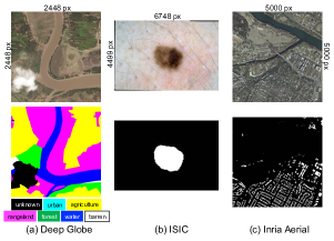
Figure 1: Three public datasets that fall into the ultra-high resolution category. DeepGlobe [11] provides satellite images with 2448$\times$2448 pixels uniformly, labeled into seven categories of land regions. ISIC [9, 10] collects dermoscopy images of size up to 6748$\times$4499 pixels, with binary labels for segmenting foreground lesions. Inria Aerial [11] provides binary masks for building/non-building areas in aerial images with 5000$\times$5000 pixels uniformly.

Our proposed model, named Collaborative Global-Local Networks (GLNet), integrates both global images and local patches, for both training and inference. GLNet has a global branch and a local branch, handling downsampled global images and cropped local patches respectively. They further interact and “modulate” each other, through deeply shared and/or mutually regularized features maps across layers. This special design enables our GLNet the capability of well-balancing its accuracy and GPU memory usage (red dots in Fig. LABEL:deep_globe_acc_mem). To further resolve the class imbalance problem that often occurs, e.g., when one is primarily interested in segmenting small foreground regions, we provide a coarse-to-fine variant of our GLNet, where the global branch provides an additional bounding box localization. The GLNet design enables the seamless integration between global contextual information and necessary local fine details, balanced by learning, to ensure accurate segmentation. It meanwhile greatly trims down the GPU memory usage, as we only operate on downsampled global images plus cropped local patches; the original ultra-high resolution image is never loaded into the GPU memory. We summarize our main contributions as follows:

• We develop a memory-efficient GLNet for the emerging new problem of ultra-high resolution image segmentation. The training requires only one 1080Ti GPU and inference requires less than 2GB GPU memory, for ultra-high resolution images of up to 30M pixels.

• GLNet can effectively and efficiently integrate global context and local high-resolution fine structures, yielding high-quality segmentation. Either local or global information is proven to be indispensable.

• We further propose a coarse-to-fine variant of GLNet to resolve the class imbalance problem in ultra-high resolution image segmentation, boosting the performance further while keeping the computation cost low.

2 Related Work

2.1 Semantic Segmentation: Quality & Efficiency

Fully convolutional network (FCN) [5] was the first CNN architecture adopted for high-quality segmentation. U-Net [6, 21, 22] used skip-connections to concatenate low-level feature to high-level ones, with an encoder-decoder architecture. Similar structures were also adopted by DeconvNet [23] and SegNet [8]. DeepLab [24, 25, 26, 3] used dilated convolution to enlarge the field of view of filters. Conditional random fields (CRF) were also utilized to model the spatial relationship. Unfortunately, these models will suffer from prohibitively high GPU memory requirements when applied to ultra-high resolution images (Fig. LABEL:deep_globe_acc_mem).

As semantic segmentation grows important in many real-time/low-latency applications (e.g. autonomous driving), efficient or fast segmentation models have recently gained more attention. ENet [27] used an asymmetric encoder-decoder structure with early downsampling, to reduce the floating point operations. ICNet [2] cascaded feature maps from multi-resolution branches under proper label guidance, together with model compression. However, these models were not customized for nor evaluated on ultra-high resolution images, and our experiments show that they did not achieve sufficiently satisfactory trade-off in such cases.

2.2 Multi-Scale and Context Aggregation

Multi-scale [24, 28, 29, 30] has proven to be powerful for segmentation, via integrating high-level and low-level features to capture patterns of different granularity. In RefineNet [31], a multi-path refinement block was utilized to combine multi-scale features via upsampling lower-resolution features. [32] adopted a Laplacian pyramid to utilize higher-level features to refine boundaries reconstructed from lower-resolution maps. Feature Pyramid Networks (FPN) [4] progressively upsampled feature maps of different scales and aggregated them in a top-down fashion. Hierarchical Auto-Zoom Net (HAZN) [29] utilized a two-step automatic zoom-in strategy to pass the coarse-stage bounding box and prediction scores to the finer stage.

Context aggregation also plays a key role in encoding the local spatial neighborhood, or even non-local information. Global pooling was adopted in ParseNet [33] to aggregate different levels of context for scene parsing. The dilated convolution and ASPP (atrous spatial pyramid pooling) module in DeepLab [25] helped enlarge the receptive field without losing feature map resolution too fast, leading to the aggregation of global contexts into local information. Similar goal was accomplished by the pyramid pooling in PSPNet [7]. In ContextNet [34], BiSeNet [35] and GUN [36], the deep/shallow branches were combined to aggregate global context and high-resolution details. [37] considered the contextual information as a long-range dependency modeled by RNNs. It is worth noting that in our GLNet, the context aggregation is adopted in both input level (global/local branch) and feature level.

2.3 Ultra-high Resolution Segmentation Datasets

We summarize three public datasets with ultra-high images (studied in Section 4). Basic information and visual examples are shown in Table 1 and Fig. 1, respectively.

The DeepGlobe Land Cover Classification dataset (DeepGlobe) [1] is the first public benchmark offering high-resolution sub-meter satellite imagery focusing on rural areas. DeepGlobe provides ground truth pixel-wise masks of seven classes: urban, agriculture, rangeland, forest, water, barren, and unknown. It contains 1146 annotated satellite images, all of size 2448$\times$2448 pixels. DeepGlobe is of significantly higher resolution and more challenging than previous land cover classification datasets.

The International Skin Imaging Collaboration (ISIC) [9, 10] dataset collects a large number of dermoscopy images. Its subset, the ISIC Lesion Boundary Segmentation dataset, consists of 2594 images from patient samples presented for skin cancer screening. All images are annotated with ground truth binary masks, indicating the locations of the primary skin lesion. Over 64% images have ultra-high resolutions: the largest image has 6682$\times$4401 pixels.

The Inria Aerial Dataset [11] covers diverse urban landscapes, ranging from dense metropolitan districts to alpine resorts. It provides 180 images (from five cities) of 5000$\times$5000 pixels, each annotated with a binary mask for building/non-building areas. Different from DeepGlobe, it splits the training/test sets by city instead of random tiles.

3 Collaborative Global-Local Networks

3.1 Motivation: Why Not Global or Local Alone

For training and inference on ultra-high resolution images with limited GPU memory, two ad-hoc ideas may come up first: downsampling the global image, or cropping it into patches. However, they both often lead to undesired artifacts and poor performance. Fig. 2(1) displays a 2448$\times$2448-pixel image, with its ground-truth segmentation in Fig. 2(2): yellow represents “agriculture”, blue “water”, and white “barren”. We then trained two FPN models: one with all images downsampled to 500$\times$500 pixels, the other with cropped patches of size 500$\times$500 pixels from original images. Their predictions are displayed in Fig. 2(3) and (4), respectively. One can observe that the former suffers from “jiggling” artifacts and inaccurate boundaries, due to the missing details from downsampling. In comparison, the latter has large areas misclassified. Note that “agriculture” and “barren” regions often visually look similar (zoom-in panels (a) and (b) in Fig. 2(1)). Therefore, the patch-based training lacks spatial contexts and neighborhood dependency information, making it difficult to distinguish between “agriculture” and “barren” using local patches only. Finally, we provide our GLNet’ prediction in Fig. 2(5) for reference: it clearly shows the advantages of leverage merits from both global and local processing.

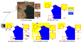
Figure 2: Example segmentation results in DeepGlobe dataset (best viewed in a high-resolution display): (1) Source image. (2) Ground-truth segmentation mask. We show predictions by (3) model trained with downsampled global images only, (4) model trained with cropped local patches only, (5) our proposed collaborative GLNet. The zoom-in panels (a) and (b) illustrate the details of local fine structures, showing the undesired grid-like artifacts and inaccurate boundaries from the global or local result alone.

3.2 GLNet Architecture

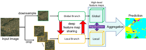
Figure 3: Overview of our proposed GLNet. The global and local branch takes downsampled and cropped images, respectively. Deep feature map sharing and feature map regularization enforce our global-local collaboration. The final segmentation is generated by aggregating high-level feature maps from two branches.

3.2.1 The Global and Local Branches

We depict our GLNet architecture in Fig. 3. Starting from the dataset of $N$ ultra-high resolution images and segmentations $\mathcal{D}=\{(\bm{I}_{i},\bm{S}_{i})\}_{i=1}^{N}$ where $\bm{I}_{i},\bm{S}_{i}\in\mathbb{R}^{H\times W}$, the global branch $\mathcal{G}$ takes down-sampled low-resolution images $\mathcal{D}^{\text{lr}}=\{(\bm{I}_{i}^{\text{lr}},\bm{S}_{i}^{\text{lr}})\}_{i=1}^{N}$, and the local branch $\mathcal{L}$ receives cropped patches from $\mathcal{D}$ with the same resolution $\mathcal{D}^{\text{hr}}=\{\{(\bm{I}_{ij}^{\text{hr}},\bm{S}_{ij}^{\text{hr}})\}_{j=1}^{n_{i}}\}_{i=1}^{N}$, where each $\bm{I}_{i}$ and $\bm{S}_{i}$ in $\mathcal{D}$ comprises $n_{i}$ patches. Note that $\bm{I}_{i}$ and $\bm{S}_{i}$ were fully cropped into patches (instead of random cropping) to facilitate both training and inference. $\bm{I}_{i}^{\text{lr}},\bm{S}_{i}^{\text{lr}}\in\mathbb{R}^{h_{1}\times w_{1}}$ and $\bm{I}_{i}^{\text{hr}},\bm{S}_{i}^{\text{hr}}\in\mathbb{R}^{h_{2}\times w_{2}}$, where $h_{1},h_{2}\ll H$, and $w_{1},w_{2}\ll W$. We adopt the same backbone for $\mathcal{G}$ and $\mathcal{L}$, both can be viewed as a cascade of convolutional blocks from layer $1$ to $L$ (Fig. 4).

During the segmentation process, the feature maps from all layers of either branch are deeply shared with the others (Section 3.2.2). Two sets of high-level feature maps are then aggregated to generate the final segmentation mask via a branch aggregation layer $f_{\text{agg}}$ (Section 3.2.3). To constrain the two branches and stabilize training, a weakly-coupled regularization is also applied to the local branch training.

3.2.2 Deep Feature Map Sharing

To collaborate with the local branch, feature maps from the global branch are first cropped at the same spatial location of the current local patch and then upsampled to match the size of the feature maps from the local branch. Next, they are concatenated as extra channels to the local branch feature maps in the same layer. In a symmetrical fashion, the feature maps from the local branch are also collected. The local feature maps are first downsampled to match the same relative spatial ratio as the patches were cropped from the large source image. Then they are merged together (in the same order as the local patches were cropped) into a complete feature map of the same size as the global branch feature map. Those local feature maps are also concatenated as channels to the global branch feature maps, before feeding into the next layer.

Fig. 4 illustrates the process of deep feature map sharing, which is applied layer-wise except the last layer of branches. The sharing direction can be either unidirectional (e.g. sharing global branch’s feature maps to local branch, $\mathcal{G}\rightarrow\mathcal{L}$) or bidirectional ($\mathcal{G}\rightleftarrows\mathcal{L}$). At each layer, the current global contextual features and local fine structural features take reference and are fused to each other.

3.2.3 Branch Aggregation with Regularization

The two branches will be aggregated through an aggregation layer $f_{\text{agg}}$, implemented as a convolutional layer of 3$\times$3 filters. It takes the high-level feature maps from the local branch’s $L^{\text{th}}$ layer $\bm{\hat{X}}_{L}^{\text{Loc}}$, and same ones from the global branch $\bm{\hat{X}}_{L}^{\text{Glb}}$, and concatenate them along the channel. The output of $f_{\text{agg}}$ will be the final segmentation output $\bm{\hat{S}}^{\text{Agg}}$. In addition to the main segmentation loss enforced on $\bm{\hat{S}}^{\text{Agg}}$, we also apply two auxiliary losses, to enforce the segmentation output from the local branch $\bm{\hat{S}}^{\text{Loc}}$ and from the global branch $\bm{\hat{S}}^{\text{Glb}}$ to be close to their corresponding segmentation maps (local patch / global downsampled), respectively, which we find helpful for stabilizing the training.

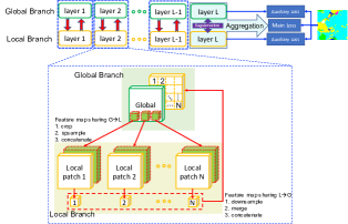
Figure 4: Deep feature map sharing between the global and local branch. At each layer, feature maps with global context and ones with local fine structures are bidirectionally brought together, contributing to a complete patch-based deep global-local collaboration. The main loss from the aggregated results and two auxiliary losses from two branches form our optimization target.

We find in practice that the local branch is prone to overfitting some strong local details, and “overriding” the learning of global branch. Therefore, we try to avoid the local branch from learning “too much faster” than the global one, by adding a weakly-coupled regularization between feature maps from the last layers of two branches. Specifically, we add the Euclidean norm penalty $\lambda\|\bm{\hat{X}}_{L}^{\text{Loc}}-\bm{\hat{X}}_{L}^{\text{Glb}}\|_{2}$ to discourage large relative changes between $\bm{\hat{X}}_{L}^{\text{Loc}}$ and $\bm{\hat{X}}_{L}^{\text{Glb}}$ with $\lambda$ empirically fixed as 0.15 in our work. This regularization is mainly designed to make local branch training “slow down” and more synchronized with global branch learning, and it only updates the parameters in local branch.

3.3 Coarse-to-Fine GLNet

For segmentation to separate foreground and background (i.e., binary masks), the foreground often takes little space in ultra-high resolution images. Such class imbalance may seriously damage the segmentation performance. Taking the ISIC dataset for example, $\sim$99% of images have more background than foreground pixels, and over 60% of images have less than 20% foreground pixels (see the blue bars in Fig. 7(1)). Many local patches will contain nothing but background pixels, which leads to ill-conditioned gradients.

A Two-Stage Refinement Solution

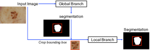
Figure 5: Two-stage segmentation. Our global branch does coarse segmentation, and for fine segmentation with the local branch we only process the bounding box foreground-centered region.

To alleviate the class imbalance, we propose a novel two-stage coarse-to-fine variant of GLNet (Fig. 5). It first applies the global branch alone to fulfill a coarse segmentation on downsampled images. A bounding box is then created for the segmented foreground region. The bounded foreground in the original full-resolution image is then fed as the input for the local branch for fine segmentation. Different from GLNet admitting parallel local-global branches, this Coarse-to-Fine GLNet admits a sequential composition of the two branches, where the feature maps only within the bounding box are first deeply shared from the global to the local branch during the bounding box refinement, and then shared back. All regions beyond the bounding box will be predicted as the background. The Coarse-to-Fine GLNet also reduces the computation cost, through selective fine-scale processing.

4 Experiments

In this section, we evaluate the performance of GLNet on the DeepGlobe and Inria Aerial datasets and evaluate the efficacy of the coarse-to-fine GLNet on the ISIC dataset. We thoroughly compare our models with other methods to show both the segmentation quality and memory efficiency. Ablation study is also carefully presented.

4.1 Implementation Details

In our work, we adopt the FPN (Feature Pyramid Network) [4] with ResNet50 [38] as our backbone. The deep feature map sharing strategy is applied on the feature maps from conv2 to conv5 blocks of ResNet50 in the bottom-up stage, and also on the feature maps from the top-down and smoothing stages in the FPN. For the final lateral connection stage in the FPN, we adopted the feature map regularization, and aggregate this stage for the final segmentation. For simplicity, both the downsampled global image and the cropped local patches share the same size, 500$\times$500 pixels. Neighboring patches have 50-pixel overlap to avoid boundary vanishing for all the convolutional layers. We use the Focal Loss [39] with $\gamma=6$ as the optimization target for both the main and two auxiliary losses. Equal weights (1.0) are assigned to the main and auxiliary losses. The feature map regularization coefficient $\lambda$ is set to 0.15.

To measure the GPU memory usage of a model, we use the command line tool “gpustat”, with the minibatch size of 1 and avoid calculating any gradients. Note that only a single GPU card is used for our training and inference.

We conduct experiments using the PyTorch framework [40]. We use the Adam optimizer [41] ($\beta_{1}=0.9$, $\beta_{2}=0.999$) with learning rate of $1\times 10^{-4}$ for training the global branch, and $2\times 10^{-5}$ for the local branch. We use a minibatch size of 6 for all training. All experiments are performed on a workstation with NVIDIA 1080Ti GPU cards.

4.2 DeepGlobe

We first apply our framework to the DeepGlobe dataset. This dataset contains 803 ultra-high resolution images (2448$\times$2448 pixels). We randomly split images into training, validation and testing sets with 455, 207, and 142 images respectively. The dense annotation contains 7 classes of landscape regions, where one class out of seven called “unknown” region is not considered in the challenge.

Table 2: Efficacy of different feature map sharing strategies evaluated on the local DeepGlobe test set. ‘Agg’ stands for the aggregation layer and ‘Fmreg’ means feature map Euclidean norm regularization. ‘$\mathcal{G}\rightarrow\mathcal{L}$’ and ‘$\mathcal{G}\rightleftarrows\mathcal{L}$’ represent feature map sharing from the global to local branch and bidirectionally between two branches respectively. ‘Shallow’ and ‘deep’ denote whether sharing feature maps in a single layer or in all layers in a model.

Model

Agg

Fmreg

$\mathcal{G}\rightarrow\mathcal{L}$

$\mathcal{G}\rightleftarrows\mathcal{L}$

mIoU (%)

Memory (MB)

shallow

deep

deep

Local only

57.3

1189

Global only

66.4

1189

GLNet

✓

69.3

1189

✓

✓

70.3

1209

✓

✓

✓

70.5

1251

✓

✓

✓

70.9

1395

✓

✓

✓

✓

71.6

1865

4.2.1 From shallow to deep feature map sharing

To evaluate the performance of our global-local collaboration strategy, we progressively upgrade our model from shallow to deep feature map sharing (Table 2). With downsampled global images or image patches alone, each branch could only achieve the mean intersection over union (mIoU) of 57.3% and 66.4% respectively. By the aggregation of the high-level feature maps from two branches and the regularization between them, the performance can be boosted to 70.3%. When we share only a single layer of feature maps from the global to the local branch (“shallow sharing”), the aggregated results increased by 0.2%, and when we upgrade to “deep sharing” where feature maps of all layers are shared, the mIoU is rocked to 70.9%. Finally, the bidirectional deep feature map sharing between two branches enables the model to yield a high mIoU of 71.6%.

This ablation study proves that, with deep and diverse feature map sharing/regularization/aggregation strategies, the global and local branch can effectively collaborate together. It is worth noting that even with the bidirectional deep feature map sharing approach (last row in Table 2), the memory usage during inference is only slightly increased from 1189MB to 1865MB.

Fig. 6 visualizes the achieved improvements with two zoom-in panels (a) and (b) showing details. There are undesired grid-like artifacts and inaccurate boundaries in the global (Fig. 6(3)) or local results (Fig. 6(4)) alone. From aggregation, shallow feature map sharing, and finally to bidirectional deep feature map sharing, progressive improvements can be observed with both significantly reduced misclassification and inaccurate boundaries.

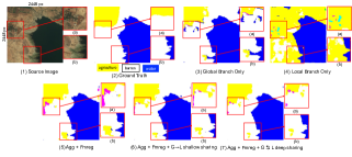
Figure 6: Example segmentation results in DeepGlobe dataset (best viewed in a high-resolution display). (1) Source image. (2) Ground truth. We show predictions by models trained with: (3) downsampled global images only, (4) cropped local patches only, (5) aggregation (‘Agg’) and feature map regularization (‘Fmreg’), (6) shallow feature map sharing, and (7) bidirectional deep feature map sharing. Improvements from (3) to (7) in the zoom-in panels (a) and (b) illustrate the details of local fine structures.

4.2.2 Accuracy and memory usage comparison

Models trained and inferenced with global images or local patches may yield different results. This is because models have different receptive fields, convolution kernel sizes, and padding strategies, which results in different suitable training/inference choices. Therefore we carefully compared models trained with these two approaches in this ablation study. We train and test a model twice (with global images or local patches each time), and then pick its best result.

Coarse comparison with fixed image/patch size

Table 3 shows that all models achieve higher mIoU under global inference, but consume very high GPU memories. Their memory usages drop in patch-based inference, but accuracies also nose dive. Only our GLNet achieves the best trade-off between mIoU and GPU memory usage. We plot the best achievable mIoU of each method in Fig. LABEL:deep_globe_acc_mem(a).

Table 3: Predicted mIoU and inference memory usage on the local DeepGlobe test set. ‘$\mathcal{G}\rightarrow\mathcal{L}$’ and ‘$\mathcal{G}\rightleftarrows\mathcal{L}$’ means feature map sharing from the global to local branch and bidirectionally between two branches respectively. Note that our GLNet does not inference with global images. See Fig. LABEL:deep_globe_acc_mem(a) for visualization.

Model	Patch Inference			Global Inference
	mIoU(%)	Memory(MB)		mIoU(%)	Memory(MB)
UNet[6]	37.3	949		38.4	5507
ICNet[2]	35.5	1195		40.2	2557
PSPNet[7]	53.3	1513		56.6	6289
SegNet[8]	60.8	1139		61.2	10339
DeepLabv3+[3]	63.1	1279		63.5	3199
FCN-8s[5]	64.3	1963		70.1	5227
	mIoU(%)			Memory(MB)
GLNet: $\mathcal{G}\rightarrow\mathcal{L}$	70.9			1395
GLNet: $\mathcal{G}\rightleftarrows\mathcal{L}$	71.6			1865

In-depth comparison with different image/patch sizes

We select FCN-8s and ICNet for in-depth evaluations with different image/patch sizes, since they achieve high mIoU and efficient memory usage respectively. We plot details of this ablation study in Fig. LABEL:deep_globe_acc_mem(b) and (c). For both FCN-8s and ICNet, higher accuracy means to sacrifice GPU memory usage, and vice versa. This proves that typical models fail to balance their segmentation quality and efficiency.

4.3 ISIC

The ISIC Lesion Boundary Segmentation Challenge dataset contains 2594 ultra-high resolution images. We randomly split images into training, validation and testing sets with 2074, 260, and 260 images respectively.

4.3.1 Coarse-to-fine segmentation

On the heavily imbalanced ISIC dataset, the global and local branch can only achieve 72.7% and 48.5% mIoU respectively. When we apply our coarse-to-fine strategy, we can clearly see a much more balanced foreground-background class ratio (red bars in Fig. 7(1)).

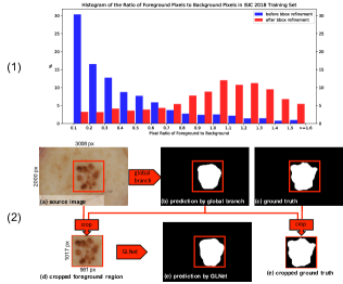
Figure 7: (1) Histogram of the ratio of foreground to background pixels (per image) in ISIC 2018 dataset. Blue bars represent ratios before global branch’s bounding box refinement, and red for ratios after the refinement, which is more balanced. (2) Visual results of coarse-to-fine segmentation. After the refinement (from (b) to (e)) the GLNet is able to capture more accurate boundaries.

By cropping a relaxed bounding box for the foreground (Section 4.2), the local branch is only trained on smaller and class-balanced images, and the cropped-out margin region is assumed as background by default. With class-balanced images, the global-to-local sharing strategy yields 73.9% mIoU, and further bidirectional sharing boosts the performance to 75.2%. In this scenario, the global branch uses a more accurate global context since there is less information loss during downsampling the cropped smaller images. This success proves that the coarse-to-fine segmentation can better capture the context information and solve the class-imbalance problem. We list the results of this ablation study in Table 4 and some visual results in Fig. 7(2).

Table 4: Efficacy of coarse-to-fine segmentation and deep feature map sharing evaluated on local ISIC test set. ‘$\mathcal{G}\rightarrow\mathcal{L}$’ and ‘$\mathcal{G}\rightleftarrows\mathcal{L}$’ represent feature map sharing direction from the global to local branch and bidirectionally between two branches respectively. ‘Bbox’ means bounding box refinement by the global branch.

Model		$\mathcal{G}\rightarrow\mathcal{L}$	$\mathcal{G}\rightleftarrows\mathcal{L}$	Bbox	mIoU (%)
Global only					70.1
Local only					48.5
GLNet		✓			72.7
		✓		✓	73.9
			✓	✓	75.2

4.3.2 Accuracy and memory usage comparison

We finally list mIoU and inference memory usage of GLNet on the local test set of the ISIC dataset in Table 5. GLNet yields mIoU 75.2% and is quantitatively better than other methods on both accuracy and memory usage.

Table 5: Predicted mIoU and inference memory usage on the local ISIC test set.

Model		mIoU (%)		Memory (MB)
ICNet[2]		33.8		1593
SegNet[8]		37.1		4213
DeepLabv3+[3]		70.5		2033
FCN-8s[5]		42.8		5238
GLNet		75.2		1921

4.4 Inria Aerial

The Inria Aerial Challenge dataset contains 180 ultra-high resolution images, each with 5000$\times$5000 pixels. We randomly split images into training, validation and testing sets with 126, 27, and 27 images respectively. Table 6 demonstrates the efficacy and efficiency of our deep feature map sharing strategy. The testing results are listed in Table 7, where our proposed GLNet yields mIoU 71.2%. Again, GLNet is quantitatively better than other methods on both accuracy and memory usage. It is worth noting that our GLNet preserves a low memory usage even for a “super” ultra-high resolution image with 5000$\times$5000 pixels.

Table 6: Efficacy of the GLNet evaluated on local Inria Aerial test set. ‘$\mathcal{G}\rightarrow\mathcal{L}$’ and ‘$\mathcal{G}\rightleftarrows\mathcal{L}$’ represent feature map sharing direction from the global to local branch and bidirectionally between two branches respectively.

Model		$\mathcal{G}\rightarrow\mathcal{L}$		$\mathcal{G}\rightleftarrows\mathcal{L}$		mIoU (%)
Global only						42.5
Local only						63.1
GLNet		✓				66.0
				✓		71.2

Table 7: Predicted mIoU and inference memory usage on local Inria Aerial test set.

Model		mIoU (%)		Memory (MB)
ICNet[2]		31.1		2379
DeepLabv3+[3]		55.9		4323
FCN-8s[5]		61.6		8253
GLNet		71.2		2663

5 Conclusions

We proposed a memory-efficient segmentation model GLNet specifically for the ultra-high resolution images. It leverages both the global context and local fine structure effectively to enhance the segmentation in the scenario of ultra-high resolution without sacrificing the GPU memory usage. We also proved that the class imbalance problem can be solved by our coarse-to-fine segmentation approach.

We believe that pursuing an optimal balance of GPU memory and accuracy is essential for the study of ultra-high resolution images, which makes our model important. Our work is pioneering this new research topic of memory-efficient segmentation of the ultra-high resolution images.

References

- [1] Ilke Demir, Krzysztof Koperski, David Lindenbaum, Guan Pang, Jing Huang, Saikat Basu, Forest Hughes, Devis Tuia, and Ramesh Raska. Deepglobe 2018: A challenge to parse the earth through satellite images. In 2018 IEEE/CVF Conference on Computer Vision and Pattern Recognition Workshops (CVPRW), pages 172–17209. IEEE, 2018.
- [2] Hengshuang Zhao, Xiaojuan Qi, Xiaoyong Shen, Jianping Shi, and Jiaya Jia. Icnet for real-time semantic segmentation on high-resolution images. In Proceedings of the European Conference on Computer Vision (ECCV), pages 405–420, 2018.
- [3] Liang-Chieh Chen, Yukun Zhu, George Papandreou, Florian Schroff, and Hartwig Adam. Encoder-decoder with atrous separable convolution for semantic image segmentation. In Proceedings of the European Conference on Computer Vision (ECCV), pages 801–818, 2018.
- [4] Tsung-Yi Lin, Piotr Dollár, Ross B Girshick, Kaiming He, Bharath Hariharan, and Serge J Belongie. Feature pyramid networks for object detection. In CVPR, volume 1, page 4, 2017.
- [5] Jonathan Long, Evan Shelhamer, and Trevor Darrell. Fully convolutional networks for semantic segmentation. In Proceedings of the IEEE conference on computer vision and pattern recognition, pages 3431–3440, 2015.
- [6] Olaf Ronneberger, Philipp Fischer, and Thomas Brox. U-net: Convolutional networks for biomedical image segmentation. In International Conference on Medical image computing and computer-assisted intervention, pages 234–241. Springer, 2015.
- [7] Hengshuang Zhao, Jianping Shi, Xiaojuan Qi, Xiaogang Wang, and Jiaya Jia. Pyramid scene parsing network. In IEEE Conf. on Computer Vision and Pattern Recognition (CVPR), pages 2881–2890, 2017.
- [8] Vijay Badrinarayanan, Alex Kendall, and Roberto Cipolla. Segnet: A deep convolutional encoder-decoder architecture for image segmentation. IEEE transactions on pattern analysis and machine intelligence, 39(12):2481–2495, 2017.
- [9] Philipp Tschandl, Cliff Rosendahl, and Harald Kittler. The ham10000 dataset, a large collection of multi-source dermatoscopic images of common pigmented skin lesions. Scientific data, 5:180161, 2018.
- [10] Noel CF Codella, David Gutman, M Emre Celebi, Brian Helba, Michael A Marchetti, Stephen W Dusza, Aadi Kalloo, Konstantinos Liopyris, Nabin Mishra, Harald Kittler, et al. Skin lesion analysis toward melanoma detection: A challenge at the 2017 international symposium on biomedical imaging (isbi), hosted by the international skin imaging collaboration (isic). In Biomedical Imaging (ISBI 2018), 2018 IEEE 15th International Symposium on, pages 168–172. IEEE, 2018.
- [11] Emmanuel Maggiori, Yuliya Tarabalka, Guillaume Charpiat, and Pierre Alliez. Can semantic labeling methods generalize to any city? the inria aerial image labeling benchmark. In IEEE International Geoscience and Remote Sensing Symposium (IGARSS). IEEE, 2017.
- [12] Marius Cordts, Mohamed Omran, Sebastian Ramos, Timo Rehfeld, Markus Enzweiler, Rodrigo Benenson, Uwe Franke, Stefan Roth, and Bernt Schiele. The cityscapes dataset for semantic urban scene understanding. In Proceedings of the IEEE conference on computer vision and pattern recognition, pages 3213–3223, 2016.
- [13] Gabriel J Brostow, Julien Fauqueur, and Roberto Cipolla. Semantic object classes in video: A high-definition ground truth database. Pattern Recognition Letters, 30(2):88–97, 2009.
- [14] Holger Caesar, Jasper Uijlings, and Vittorio Ferrari. Coco-stuff: Thing and stuff classes in context. In Proceedings of the IEEE Conference on Computer Vision and Pattern Recognition, pages 1209–1218, 2018.
- [15] Mark Everingham, Luc Van Gool, Christopher KI Williams, John Winn, and Andrew Zisserman. The pascal visual object classes (voc) challenge. International journal of computer vision, 88(2):303–338, 2010.
- [16] Steven Ascher and Edward Pincus. The filmmaker’s handbook: A comprehensive guide for the digital age. Penguin, 2007.
- [17] Paul Lilly. Samsung launches insanely wide 32:9 aspect ratio monitor with hdr and freesync 2. https://www.pcgamer.com/samsung-launches-a-massive-49-inch-ultrawide-hdr-monitor-with-freesync-2/, 2017.
- [18] Digital Cinema Initiatives. Digital cinema system specification, version 1.3. http://dcimovies.com/specification/DCI_DCSS_Ver1-3_2018-0627.pdf, 2018.
- [19] Michele Volpi and Devis Tuia. Dense semantic labeling of subdecimeter resolution images with convolutional neural networks. IEEE Transactions on Geoscience and Remote Sensing, 55(2):881–893, 2017.
- [20] Alexandre Robicquet, Amir Sadeghian, Alexandre Alahi, and Silvio Savarese. Learning social etiquette: Human trajectory understanding in crowded scenes. In European conference on computer vision, pages 549–565. Springer, 2016.
- [21] Ding Liu, Bihan Wen, Xianming Liu, Zhangyang Wang, and Thomas S Huang. When image denoising meets high-level vision tasks: a deep learning approach. In Proceedings of the 27th International Joint Conference on Artificial Intelligence, pages 842–848. AAAI Press, 2018.
- [22] Ding Liu, Bihan Wen, Jianbo Jiao, Xianming Liu, Zhangyang Wang, and Thomas S Huang. Connecting image denoising and high-level vision tasks via deep learning. arXiv preprint arXiv:1809.01826, 2018.
- [23] Hyeonwoo Noh, Seunghoon Hong, and Bohyung Han. Learning deconvolution network for semantic segmentation. In Proceedings of the IEEE international conference on computer vision, pages 1520–1528, 2015.
- [24] Liang-Chieh Chen, George Papandreou, Iasonas Kokkinos, Kevin Murphy, and Alan L Yuille. Semantic image segmentation with deep convolutional nets and fully connected crfs. arXiv preprint arXiv:1412.7062, 2014.
- [25] Liang-Chieh Chen, George Papandreou, Iasonas Kokkinos, Kevin Murphy, and Alan L Yuille. Deeplab: Semantic image segmentation with deep convolutional nets, atrous convolution, and fully connected crfs. IEEE transactions on pattern analysis and machine intelligence, 40(4):834–848, 2018.
- [26] Fisher Yu and Vladlen Koltun. Multi-scale context aggregation by dilated convolutions. arXiv preprint arXiv:1511.07122, 2015.
- [27] Adam Paszke, Abhishek Chaurasia, Sangpil Kim, and Eugenio Culurciello. Enet: A deep neural network architecture for real-time semantic segmentation. arXiv preprint arXiv:1606.02147, 2016.
- [28] Liang-Chieh Chen, Yi Yang, Jiang Wang, Wei Xu, and Alan L Yuille. Attention to scale: Scale-aware semantic image segmentation. In Proceedings of the IEEE conference on computer vision and pattern recognition, pages 3640–3649, 2016.
- [29] Fangting Xia, Peng Wang, Liang-Chieh Chen, and Alan L Yuille. Zoom better to see clearer: Human and object parsing with hierarchical auto-zoom net. In European Conference on Computer Vision, pages 648–663. Springer, 2016.
- [30] Bharath Hariharan, Pablo Arbeláez, Ross Girshick, and Jitendra Malik. Hypercolumns for object segmentation and fine-grained localization. In Proceedings of the IEEE conference on computer vision and pattern recognition, pages 447–456, 2015.
- [31] Guosheng Lin, Anton Milan, Chunhua Shen, and Ian Reid. Refinenet: Multi-path refinement networks for high-resolution semantic segmentation. In Proceedings of the IEEE conference on computer vision and pattern recognition, pages 1925–1934, 2017.
- [32] Golnaz Ghiasi and Charless C Fowlkes. Laplacian pyramid reconstruction and refinement for semantic segmentation. In European Conference on Computer Vision, pages 519–534. Springer, 2016.
- [33] Wei Liu, Andrew Rabinovich, and Alexander C Berg. Parsenet: Looking wider to see better. arXiv preprint arXiv:1506.04579, 2015.
- [34] Rudra PK Poudel, Ujwal Bonde, Stephan Liwicki, and Christopher Zach. Contextnet: Exploring context and detail for semantic segmentation in real-time. arXiv preprint arXiv:1805.04554, 2018.
- [35] Changqian Yu, Jingbo Wang, Chao Peng, Changxin Gao, Gang Yu, and Nong Sang. Bisenet: Bilateral segmentation network for real-time semantic segmentation. In Proceedings of the European Conference on Computer Vision (ECCV), pages 325–341, 2018.
- [36] Davide Mazzini. Guided upsampling network for real-time semantic segmentation. arXiv preprint arXiv:1807.07466, 2018.
- [37] Francesco Visin, Marco Ciccone, Adriana Romero, Kyle Kastner, Kyunghyun Cho, Yoshua Bengio, Matteo Matteucci, and Aaron Courville. Reseg: A recurrent neural network-based model for semantic segmentation. In Proceedings of the IEEE Conference on Computer Vision and Pattern Recognition Workshops, pages 41–48, 2016.
- [38] Kaiming He, Xiangyu Zhang, Shaoqing Ren, and Jian Sun. Deep residual learning for image recognition. In Proceedings of the IEEE conference on computer vision and pattern recognition, pages 770–778, 2016.
- [39] Tsung-Yi Lin, Priyal Goyal, Ross Girshick, Kaiming He, and Piotr Dollár. Focal loss for dense object detection. IEEE transactions on pattern analysis and machine intelligence, 2018.
- [40] Adam Paszke, Sam Gross, Soumith Chintala, Gregory Chanan, Edward Yang, Zachary DeVito, Zeming Lin, Alban Desmaison, Luca Antiga, and Adam Lerer. Automatic differentiation in pytorch. In NIPS-W, 2017.
- [41] Diederik P Kingma and Jimmy Ba. Adam: A method for stochastic optimization. arXiv preprint arXiv:1412.6980, 2014.
- [42] Meet P Shah. Semantic segmentation architectures implemented in pytorch. https://github.com/meetshah1995/pytorch-semseg, 2017.
- [43] Kazuto Nakashima. Pytorch implementation of deeplab v2 (resnet). https://github.com/kazuto1011/deeplab-pytorch, 2018.