Nuclear Dominated Accretion Flows in Two Dimensions. II. Ejecta dynamics and nucleosynthesis for CO and ONe white dwarfs

Abstract

We study mass ejection from accretion disks formed in the merger of a white dwarf with a neutron star or black hole. These disks are mostly radiatively-inefficient and support nuclear fusion reactions, with ensuing outflows and electromagnetic transients. Here we perform time-dependent, axisymmetric hydrodynamic simulations of these disks including a physical equation of state, viscous angular momentum transport, a coupled $19$-isotope nuclear network, and self-gravity. We find no detonations in any of the configurations studied. Our global models extend from the central object to radii much larger than the disk. We evolve these global models for several orbits, as well as alternate versions with an excised inner boundary to much longer times. We obtain robust outflows, with a broad velocity distribution in the range $10^{2}-10^{4}$ km s^-1. The outflow composition is mostly that of the initial white dwarf, with burning products mixed in at the $\lesssim 10-30\%$ level by mass, including up to $\sim 10^{-2}M_{\odot}$ of ⁵⁶Ni. These heavier elements (plus ⁴He) are ejected within $\lesssim 40^{\circ}$ of the rotation axis, and should have higher average velocities than the lighter elements that make up the white dwarf. These results are in broad agreement with previous one- and two-dimensional studies, and point to these systems as progenitors of rapidly-rising ($\sim$ few day) transients. If accretion onto the central BH/NS powers a relativistic jet, these events could be accompanied by high energy transients with peak luminosities $\sim 10^{47}-10^{50}$ erg s^-1 and peak durations of up to several minutes, possibly accounting for events like CDF-S XT2.

1 Introduction

Over the past decade, optical transient surveys have uncovered new types of relatively rare events with properties intermediate between supernovae and classical novae (e.g., Kulkarni 2012), and which have yet to be conclusively associated with a progenitor system. Examples include Ca-rich transients (Perets et al., 2010; Kasliwal et al., 2012), type Iax supernovae (e.g., Foley et al. 2013), and rapidly-evolving blue transients (e.g., Drout et al. 2014).

Mergers of white dwarfs (WD) with neutron stars (NS) or stellar-mass black holes (BH) are expected to generate transients, but theoretical predictions about their observational signatures are not well developed yet. The key difficulty is the wide range of scales and physical processes involved in the problem, in contrast to mergers of similarly-sized objects (e.g., WD-WD, or NS-NS/BH) which are more tractable and for which observational predictions are more mature (e.g., Dan et al. 2014; Fernández & Metzger 2016).

Observationally, there are at least 20 confirmed galactic WD-NS binaries plus a few dozen more candidates (van Kerkwijk et al., 2005). However, only a few of these systems will merge within a Hubble time (e.g., Lorimer 2008). Merger rates are predicted to be in the range $10^{-6}$-$10^{-4}$ per year in the Milky Way, (e.g., Kim et al. 2004; O’Shaughnessy & Kim 2010) with the most frequent systems expected to contain CO and ONe WDs (Toonen et al., 2018). At present, only one candidate WD-BH binary is known in the Galaxy (Bahramian et al., 2017).

On the theoretical side, Fryer et al. (1999) considered WD-BH mergers as progenitors of long gamma-ray bursts. They explored the dynamics of disk formation during unstable Roche lobe overflow in circular orbits around stellar-mass BHs using Smooth Particle Hydrodynamc (SPH) simulations with nuclear burning, and predicted the accretion power expected from the resulting disk using analytical arguments (see also King et al. 2007). The disruption and disk formation process has also been explored by Paschalidis et al. (2011) and Bobrick et al. (2017) with time-dependent simulations. More extensive theoretical work exists in the context of tidal disruption of WDs on parabolic orbits around BHs (Luminet & Pichon, 1989; Rosswog et al., 2009; MacLeod et al., 2016; Kawana et al., 2018). Thermonuclear burning due to tidal pinching of the WD and/or tidal tail intersection are commonly found, although most existing work considers massive ($\geq 100M_{\odot}$) BHs with the exception of Kawana et al. (2018), who obtains explosions with BHs of mass $10M_{\odot}$.

Metzger (2012) explored the evolution of the torus formed during a quasi-circular WD-NS/BH merger using a steady-state, height-integrated model. Results showed that nuclear reactions are important compared to viscous heating, and that the radiatively-inefficient nature of these disks should result in significant outflows. The importance of nuclear burning led Metzger (2012) to coin the term Nuclear-Dominated Accretion Flows (NuDAF) for this regime. The burning of increasingly heavier elements as they accrete deeper into the gravitational potential generates an onion-shell-like stratification of composition in radius, with non-trivial amounts of ⁵⁶Ni production as a possible outcome. A similar analysis has recently been applied to accretion disks in X-ray binaries and supermassive black holes (Datta & Mukhopadhyay, 2019).

The time-dependent evolution of height-integrated disks was carried out by Margalit & Metzger (2016, hereafter MM16) using a prescribed outflow model. A systematic parameter exploration showed that disks from CO WDs evolve in a self-similar, quasi steady-state fashion that is relatively robust to parameter variations. Outflow velocities were found to be $\sim 10^{4}$ km s^-1, with $\sim 10^{-3}M_{\odot}$ of radioactive ⁵⁶Ni produced. At very late times, these disks could in principle be a formation site of planets around the NS (Margalit & Metzger, 2017).

Fernández & Metzger (2013b, hereafter Paper I) performed global two-dimensional hydrodynamic simulations of the accretion disk using an ideal gas equation of state, parameterized nuclear burning, and viscous angular-momentum transport. Results showed that turbulence-aided detonations of the disk are possible during the first few orbits if the nuclear energy release is significant compared to the local gravitational potential. Non-exploding cases yielded robust quasi-steady outflows, as expected from the radiatively inefficient character of the disk. A key uncertainty in these results was the robustness of detonations when a more realistic equation of state that includes radiation pressure is taken into account. Recently, Zenati et al. (2019) has reported two-dimensional time-dependent simulations of the disk including a physical equation of state, a coupled 19-isotope nuclear reaction network, viscous angular momentum transport, and self-gravity. Simulations are followed for a few orbits at the initial disk radius ($\sim 100$ s) and robust outflows are also found, with properties consistent with previous 1D studies. Detonations are also reported.

Here we study the evolution of the disk with global two-dimensional axisymmetric simulations, focusing on the properties of the disk outflow in the case of the most common CO and ONe WDs. We improve upon Paper I by including a physical equation of state, a fully-coupled nuclear reaction network, and self-gravity. We also improve on previous work by resolving all spatial scales down to the compact object surface over short times (few $100$ s), and also follow the outer disk for much longer times ($\sim$ hr) with an excised boundary. Study of He-WD/NS binaries is left for future work.

The paper is structured as follows. Section 2 describes the numerical method employed and the parameter space surveyed. Section 3 presents our results. Section 4 summarizes our conclusions and discusses observational implications. The Appendices contain a description of the self-gravity implementation, the initial conditions for the disk, and a method to obtain the accretion rate at the central object.

2 Methods

2.1 Physical Model

We consider accretion disks formed during the tidal disruption of a white dwarf by a neutron star or a black hole via unstable mass transfer. Following Metzger (2012), Paper I, and MM16, we assume that nuclear burning is not dynamical during the merger itself, and place the disk at the circularization radius (Eggleton, 1983)

$$R_{\rm t}=\frac{R_{\rm WD}}{(1+q)}\frac{0.6q^{2/3}+\ln(1+q^{1/3})}{0.49q^{2/3}}$$ (1)

where $R_{\rm WD}$ is the radius of the white dwarf before disruption, which depends on the white dwarf mass $M_{\rm WD}$ and composition (e.g., Nauenberg 1972) and $q=M_{\rm WD}/M_{\rm c}$ is the mass ratio of the binary, with $M_{\rm c}$ the mass of the other compact object (neutron star or black hole). Mass transfer should be unstable for most CO and ONe WDs (e.g., Bobrick et al. 2017).

Outside the immediate vicinity of the central compact object, where neutrino or photodissociation losses from the disk can be important, the disk is radiatively inefficient. Evolution occurs on a viscous timescale at the initial torus radius $R_{\rm t}$ by the action of angular momentum transport processes, which include magnetic turbulence and perhaps also gravitational instabilities (MM16). While our models include self-gravity, they are axisymmetric and therefore gravitational torques are not accounted for. Also, we do not include magnetic fields, and instead parameterize angular momentum transport via a viscous shear stress. See Paper I for a more extended discussion of the validity of these approximations.

2.2 Equations and Numerical Method

We solve the equations of mass, momentum, energy, and chemical species conservation in axisymmetric spherical polar coordinates $(r,\theta)$, with source terms due to gravity, shear viscosity, nuclear reactions, and charged-current neutrino emission:

$$\frac{\partial\rho}{\partial t}+\nabla\cdot(\rho\mathbf{v}_{p}) = 0$$ (2)

$$\frac{d\mathbf{v}_{p}}{dt}+\frac{1}{\rho}\nabla p = -\nabla\Phi$$ (3)

$$\rho\frac{dj}{dt} = r\sin\theta\,(\nabla\cdot\mathbf{T})_{\phi}$$ (4)

$$\rho\frac{de_{\rm int}}{dt}+p\nabla\cdot\mathbf{v}_{p} = \frac{1}{\rho\nu}\mathbf{T}:\mathbf{T}+\rho\left(\dot{Q}_{\rm nuc}-\dot{Q}_{\rm cool}\right)$$ (5)

$$\nabla^{2}\Phi = 4\pi G\rho+\nabla^{2}\Phi_{\rm c}$$ (6)

$$\frac{\partial\mathbf{X}}{\partial t} = \mathbf{\Theta}(\rho,e_{\rm int},\mathbf{X})+\mathbf{\Gamma}_{\rm cc}$$ (7)

where $d/dt\equiv\partial/\partial t+\mathbf{v_{\rm p}}\cdot\nabla$, and $\rho$, $\mathbf{v}_{\rm p}$, $j$, $p$, $e_{\rm int}$, $\Phi$, and $\mathbf{X}$ are respectively the fluid density, poloidal velocity, specific angular momentum in the $z$-direction, total pressure, specific internal energy, gravitational potential, and mass fractions of the isotopes considered ($\sum_{i}X_{i}=1$). Explicit source terms include the viscous stress tensor for azimuthal shear, with non-vanishing components

$$T_{r\phi} = \rho\nu\,\frac{r}{\sin\theta}\frac{\partial}{\partial r}\left(\frac{j}{r^{2}}\right)$$ (8)

$$T_{\theta\phi} = \rho\nu\,\frac{\sin\theta}{r^{2}}\frac{\partial}{\partial\theta}\left(\frac{j}{\sin^{2}\theta}\right),$$ (9)

the nuclear heating rate per unit volume $\dot{Q}_{\rm nuc}$, and the neutrino cooling rate per unit volume $\dot{Q}_{\rm cool}$. In equation (6), we separate the gravitational potential of the central object $\Phi_{\rm c}$ from that generated by the disk density field. There is also an implicit source term in the expansion of $(\mathbf{v_{\rm p}}\cdot\nabla)\mathbf{v}_{\rm p}$ in spherical coordinates (left hand side of equation 3), which contains a centrifugal acceleration that depends on $j$:

$$\mathbf{f}_{c}=\frac{j^{2}}{(r\,\sin\theta)^{3}}\left[\sin\theta\hat{r}+\cos\theta\hat{\theta}\right].$$ (10)

The system of equations (2)-(7) is closed with the Helmholtz equation of state (Timmes & Swesty, 2000), the 19-isotope nuclear reaction network $\mathbf{\Theta}$ of Weaver et al. (1978), which provides a cost-effective description of energy generation by fusion and losses from photodissociation and thermal neutrino emission ($\dot{Q}_{\rm nuc}$), and an alpha-viscosity prescription (Shakura & Sunyaev, 1973)

$$\nu=\alpha\frac{p}{\rho\,\Omega_{\rm K}},$$ (11)

where $\alpha$ is a free parameter and $\Omega_{\rm K}$ is the Keplerian frequency. In addition to the neutrino losses included in the nuclear network (Itoh et al., 1996), neutrino emission via charged-current weak interactions is included (as described in Fernández et al. 2019), adding a cooling term ($\dot{Q}_{\rm cool}$) and an extra source term for the mass fraction of neutrons and protons ($\mathbf{\Gamma}_{\rm cc}$).

We use FLASH3 (Fryxell et al., 2000; Dubey et al., 2009) to evolve the system of equations (2)-(7) with the dimensionally-split version of the Piecewise Parabolic Method (PPM, Colella & Woodward 1984). The modifications to the code required to evolve accretion disks with a viscous shear stress are described in Fernández & Metzger (2013a) and Paper I. Source terms are applied in between updates by the hydrodynamic solver (operator-split). The 19-isotope nuclear reaction network is that included in FLASH3; we use it with the MA28 sparse matrix solver and Bader-Deuflhard variable time stepping method (e.g., Timmes 1999). A time step limiter

$$\Delta t_{\rm burn}<0.1\frac{e_{\rm int}}{|\dot{Q}_{\rm nuc}|}$$ (12)

is imposed for nuclear burning, in addition to the standard Courant, heating, and viscous time step restrictions.

Self-gravity is implemented using the algorithm of Müller & Steinmetz (1995), with a customized version for non-uniform spherical grids. The implementation and testing of this component is described in Appendix A. The gravitational potential generated by the central object $\Phi_{\rm c}$ is modeled as a pseudo-Newtonian point mass $M_{\rm c}$, with a spin-dependent event-horizon (Artemova et al., 1996; Fernández et al., 2015).

The computational domain extends from an inner radius $R_{\rm in}$ to an outer radius $R_{\rm max}$, with the grid logarithmically spaced with $64$ cells per decade in radius. The full range of polar angles $[0,\pi]$ is covered with $56$ points equispaced in $\cos\theta$. The effective resolution at the equatorial plane is $\Delta r/r\simeq 0.037\simeq\Delta\theta\simeq 2^{\circ}$. One model is evolved at twice the resolution in radius and angle to test convergence (§2.4).

The boundary conditions are reflecting in polar angle and outflow at $r=R_{\rm max}$. At $r=R_{\rm in}$, we use a reflecting boundary condition when resolving the neutron star at the center, otherwise we set this boundary to outflow. The angular momentum is set to have a stress-free boundary condition at $r=R_{\rm in}$, except in the case when the NS is assumed to be spinning, in which case a finite stress is imposed. The boundary condition for the gravitational potential is such that it vanishes at $r\to\infty$.

2.3 Initial Conditions

The initial condition is an equilibrium torus with constant entropy, angular momentum, and composition. In a realistic system, this initial state would be determined by the dynamics of Roche lobe overflow, which requires a fully three-dimensional simulation of the merger dynamics until the disk settles into a nearly axisymmetric state. In practice, the thermal time due to viscous heating in our disks is a few orbits, or about $\sim 1/10$ of the viscous time, which means that for the timescales of interest, the thermodynamics becomes quickly set by viscous heating and nuclear burning. For systems in which a thermonuclear runaway is expected early on (i.e., ONe WD + NS mergers), the initial conditions are more important than in the systems we consider here.

Table 1: Parameters of models evolved. Columns from left to right show model name, WD mass, central object mass, radius of initial torus density maximum, initial WD composition, initial torus distortion parameter (equation 45), viscosity coefficient (equation 11), radius of inner boundary, number of cells per decade in radius $n_{\rm r}$ and total number of cells in $\theta$-direction ($n_{\rm\theta}$), type of inner radial boundary condition (out: outflow, ref: reflecting), NS spin period $p_{\rm sp}$ or dimensionless BH spin $\chi$, and maximum simulated time.

Model	$M_{\rm wd}$	$M_{\rm c}$	$R_{\rm t}$	Mass Fractions	d	$\alpha$	$R_{\rm in}$	$(n_{\rm r},n_{\rm\theta})$	BC	$p_{\rm sp}/\chi$	$t_{\rm max}$
	$(M_{\odot})$	$(M_{\odot})$	($10^{9}$ cm)	C/O/He/Ne			($10^{7}$ cm)				(s)
CO+NS(l)	0.6	1.4	2	$0.50$/$0.50$/$0.0$/$0.0$	1.5	0.03	2	(64,56)	out	0	4,123
CO+NS(l-hr)								(128,112)
CO/He+NS(l)				$0.45$/$0.45$/$0.1$/$0.0$				(64,56)
ONe+BH(l)	1.2	5.0	1	$0.00$/$0.60$/$0.0$/$0.4$			1				887
CO+NS(s)	0.6	1.4	2	$0.50$/$0.50$/$0.0$/$0.0$	1.5	0.03	0.1	(64,56)	ref	0	245
CO/He+NS(s)				$0.45$/$0.45$/$0.1$/$0.0$							215
ONe+BH(s)	1.2	5.0	1	$0.00$/$0.60$/$0.0$/$0.4$			0.3		out		50
CO+NS(s-vs)	0.6	1.4	2	$0.50$/$0.50$/$0.0$/$0.0$	1.5	0.10	0.1	(64,56)	ref	0	110
CO+NS(s-sp)						0.03				2 ms	170
ONe+BH(s-sp)	1.2	5.0	1	$0.00$/$0.60$/$0.0$/$0.4$			0.17		out	0.8	31

The torus is initially constructed using only the gravity of the central object ($\Phi_{\rm c}$), for which a semi-analytic formulation is straightforward (e.g., Papaloizou & Pringle 1984; Fernández & Metzger 2013a). This torus is then relaxed with self-gravity, by evolving it without any other source terms for 20 orbits at $r=R_{\rm t}$. A detailed description of this procedure is provided in Appendix B.

Initial tori are described by their mass ($M_{\rm WD}$), radius of maximum density ($R_{\rm t}$, equation 1), entropy (or $H/R=c_{\rm i}/\Omega_{\rm K}$ at density maximum, with $c_{\rm i}=\sqrt{p/\rho}$), angular momentum profile (constant), and composition. The orbital time at $r=R_{\rm t}$ is given by

$$t_{\rm orb}\simeq 40\,\textrm{s}\,\left(\frac{R_{\rm t}}{10^{9.3}\textrm{cm}}\right)^{3/2}\left(\frac{1.4M_{\odot}}{M_{\rm c}}\right)^{1/2},$$ (13)

and the viscous time at the same location is

$$t_{\rm vis}\simeq 900\,\textrm{s}\,\left(\frac{0.03}{\alpha}\right)\left(\frac{0.5}{\rm H/R}\right)^{2}\left(\frac{R_{\rm t}}{10^{9.3}\textrm{cm}}\right)^{3/2}\left(\frac{1.4M_{\odot}}{M_{\rm c}}\right)^{1/2}.$$ (14)

The torus is initially surrounded by a low-density adiabatic atmosphere with hydrogen composition. This ambient density profile is set to $10^{-3}$ g cm^-3 inside $r=4R_{\rm t}$ for most models, and decays as $r^{-2}$ outside this radius. In some cases we add a $r^{-0.5}$ dependence of this ambient inside $r=4R_{\rm t}$ whenever numerical problems at the inner radial boundary are encountered; this value is small enough it does not affect the dynamics of the outflow. A density floor is set at 90% of the initial ambient value. A constant floor of pressure ($10^{8}$ erg cm^-3) about an order of magnitude lower than the lowest ambient value (near the outer boundary) is used to prevent numerical problems around the torus edges at early times and near the rotation axis at the inner boundary once an evacuated funnel forms. A constant floor or temperature ($3\times 10^{4}$ K) is also used to prevent the code from reaching the lowest tabulated temperature in the Helmholtz EOS. The choice of floors is low enough that results do not depend on it. When computing mass ejection and accretion, the ambient matter is excluded, and material coming from the disk has densities much higher than this initial ambient gas.

2.4 Models Evolved

All of our models are described in Table LABEL:t:models. Given the large dynamic range in radius ($\gtrsim 10^{3}$) between the initial disk radius $R_{t}$ and the characteristic size of the central compact object, and the fact that our time step is limited by the Courant condition at the smallest radius in the simulation, we evolve two types of models.

The first group sets the inner boundary radius at $R_{\rm in}=10^{-2}R_{\rm t}\sim 10^{7}$ cm, allowing evolution to long timescales ($\sim$ few $t_{\rm vis}$) but not resolving the regions from where the fastest outflows are launched and where ⁵⁶Ni is produced for a central NS. These models thus probe nucleosynthesis of intermediate-mass elements and the time-dependence of mass ejection on long timescales (as in Paper I). These models have “(l)” appended to their names, for “large inner boundary”.

The group consists of our fiducial WD+NS model, CO+NS(l), a $0.6M_{\odot}$ CO WD around a $1.4M_{\odot}$ NS with a viscosity of $\alpha=0.03$ and an initial entropy of $3k_{\rm B}$ per nucleon (c.f. Appendix B). To test the effect of a small admixture of helium, we include model CO/He+NS(l), which is identical to the fiducial case except that the initial abundances of helium, carbon, and oxygen are $10\%$, $45\%$, and $45\%$, respectively. Model ONe+BH(l) probes a more massive ONe WD ($1.2M_{\odot}$) around a $5M_{\odot}$ BH, with otherwise identical parameters. Finally, model CO+NS(l-hr) is identical to the fiducial case but with twice the resolution in radius and angle, to probe the degree of convergence of our results. All these models are evolved to $t=100t_{\rm orb}\simeq 4t_{\rm vis}$.

The second group of models (“small inner boundary”, or “(s)” for short) resolve the central compact object but are evolved for a shorter amount of time ($\sim$ several $t_{\rm orb}$). Model CO+NS(s) corresponds to the fiducial case but now with an inner reflecting radial boundary at $10$ km. Likewise, model CO/He+NS(s) probes the hybrid WD while resolving the neutron star. In both cases, the neutron star is assumed to be non-rotating. Model ONe+BH(s) extends the domain of the corresponding large inner boundary BH model to a radius midway between the innermost stable circular orbit (ISCO) and horizon. The BH is assumed to be non-spinning.

We include additional models that probe parameter variations among the small inner boundary set. CO+NS(s-vs) increases the alpha viscosity parameter from $\alpha=0.03$ to $0.1$. Model CO+NS(s-sp) adds a spin period of $2$ ms to the NS and imposes a finite viscous stress at this boundary, to probe energy release at the boundary layer. Finally, model ONe+BH(s-sp) adds a dimensionless spin of $\chi=0.8$ to the BH, extending accretion to smaller radii (the inner boundary is again placed midway between the new ISCO and horizon radii).

For small boundary models, we first evolve the disk with a large inner boundary to save computational time in this early phase, until the disk material reaches this larger inner boundary. The result is then remapped into a grid that extends the inner boundary further inward, with the process being repeated for each additional order of magnitude that $R_{\rm in}$ decreases.

3 Results

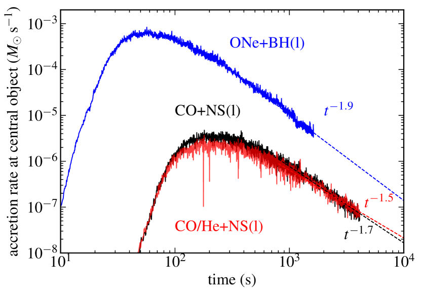
Figure 1: Mass accretion rate at the central object inferred from the three large boundary models by following the procedure described in Appendix C. The dashed lines show power-law fits in time.

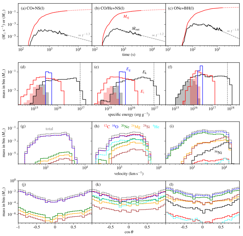
Figure 2: Mass ejection properties of models with a large inner boundary ($R_{\rm in}=0.01R_{\rm t}$), as labeled. Top: Mass loss rate (solid black) in unbound material as a function of time, measured at a radius $r_{\rm out}=30R_{\rm t}$ ($\simeq 6\times 10^{10}$ cm for the fiducial CO+NS model) and cumulative unbound mass ejected at this radius (solid red). The gray dashed line shows a power-law fit to the mass loss rate, which when extrapolated yields a prediction for the total mass ejected (red dashed, equation 16). Second row: Final mass histograms of unbound material as a function of specific kinetic energy (black), internal energy (red), and gravitational energy (blue) at $r=r_{\rm out}$. The vertical dashed line shows the specific gravitational binding energy at the initial torus density peak, ignoring self-gravity ($GM_{\rm c}/R_{\rm t}$), and the shaded histograms correspond to material with positive Bernoulli parameter but negative total energy (i.e., marginally unbound). Third row: Final mass histograms in unbound material at $r=r_{\rm out}$ as a function of radial velocity, for various species, as labeled. Bottom: mass histograms as a function of polar angle, for various species. Note that these models do not account for the mass ejected from $r<0.01R_{\rm t}$, and therefore the results shown correspond to lower limits to the ejected mass and its radial velocity (see §3.3).

3.1 Mass ejection on long timescales

Over the first few orbits at $r=R_{\rm t}$, the equilibrium initial tori begin accreting to small radius while simultaneously transporting angular momentum outward. The absence of cooling during this initial stage leads to vigorous convection. This early phase of evolution is nearly identical to the quiescent models of Paper I, with quantitative details that depend on the parameters of the system. Figure 1 shows the accretion rate at the central object for the three large inner boundary models that remove the regions with $r<0.01R_{\rm t}$ to allow for a longer evolution [CO+NS(l), CO/He+NS(l), and ONe+BH(l)]. The accretion rate reaches a peak around 5-6 orbits at $r=R_{\rm t}$ ($\simeq 200$ s for the NS models, and $\simeq 35$ s for the BH model).

None of our large boundary models detonate during the initial viscous spreading of the equilibrium torus nor at later stages. This stands in contrast to some of the results of Paper I, which used parametric nuclear reactions, an ideal equation of state, and point mass gravity. At higher temperatures, the increasing contribution of radiation pressure results in more moderate increases in the temperature at small disk radii, preventing nuclear burning from ever causing a thermonuclear runaway (see §3.5 for a more detailed discussion of this effect). Inclusion of self-gravity only increases the density by a factor of $\sim 2$ and moves the radius of the torus density peak inward by a few percent relative to using only point mass gravity (Appendix B). The quantitative difference in the evolution once source terms are included is minor. As a more extreme example, we evolved a test fiducial model in which the initial condition obtained with point mass gravity is not relaxed for self-gravity. While stronger nuclear burning is obtained in some regions of the disk due to radial oscillations, a detonation is not obtained within $2$ orbits.

The onset of convection is also accompanied by outflows from the disk, which continue until the end of all simulations. We consider matter to be unbound from the disk when its Bernoulli parameter

$$b=\frac{1}{2}\left[v_{r}^{2}+v_{\theta}^{2}+\frac{j^{2}}{(r\sin\theta)^{2}}\right]+e_{\rm int}+\frac{p}{\rho}+\Phi$$ (15)

is positive. This criterion considers the conversion of thermal energy into kinetic energy by adiabatic expansion, and is useful when measuring the outflow at radii not much larger than the disk. The unbound mass outflow rate at a radius $r_{\rm out}=30R_{\rm t}$ is shown in Figure 2 for the three large inner boundary models. Peak outflow is reached around 15 orbits at $r=R_{\rm t}$, with a subsequent decay with time (after $t\simeq t_{\rm vis}$) that follows an approximate power-law.

By the time we stop our large inner boundary models ($100$ orbits at $r=R_{\rm t}$, see Table LABEL:t:models for values in s), mass ejection is not yet complete. Nevertheless, given the power-law dependence with time of the outflow rate, we can estimate the final ejecta mass by extrapolating forward in time assuming that the same power law continues without changes (see also MM16). If this assumption holds, the extrapolation is a lower limit on the total ejecta mass, because it does not include the contribution from $r<0.01R_{\rm t}$, which is quite significant when a NS sits at the center (§3.3.1). If the mass outflow rate at some radius is $\dot{M}_{\rm out}\propto t^{-\delta}$ ($\delta>0$), then we can write for $t>t_{0}$

$$M_{\rm ej}(t)=M_{\rm ej,0}+\frac{1}{\delta-1}\dot{M}_{\rm out,0}t_{0}\left[1-\left(\frac{t}{t_{0}}\right)^{1-\delta}\right]$$ (16)

with $M_{\rm ej,0}$ and $\dot{M}_{\rm out,0}$ the ejected mass and outflow rate at $t=t_{0}\sim t_{\rm vis}$, after which the power-law dependence holds. For a finite value at $t\to\infty$, we need $\delta>1$. Figure 2 shows $M_{\rm ej}$ as a function of time. The resulting exponents are $\delta\simeq\{1.3,1.2,1.8\}$ for models CO+NS(l), CO/He+NS(l), and ONe+BH(l), respectively, leading to a finite asymptotic value in all three cases. All mass ejection results are shown in Table LABEL:t:results. The asymptotic ejecta masses for the large boundary models are $60-70\%$ of the initial WD mass before including the contribution from $r<0.01R_{\rm t}$. Over the short timescales that small boundary models run, they eject about twice more mass when counted to the same radius and time than large boundary models (§3.3). A simple scaling of the asymptotic ejecta by this factor would exceed the initial WD mass, which indicates that (1) most of the WD mass is indeed likely to be ejected, but that (2) the time exponents of the outflow are also likely to change with time and/or be different than those derived from the large boundary models. Upper limits to the ejected mass can be obtained by subtracting the asymptotic accreted mass at the compact object (Figure 1) from the WD mass. These accreted masses are $\simeq 3\times 10^{-3}M_{\odot}$ for the WD+NS models, and $0.12M_{\odot}$ for the ONe+BH model.

Figure 2 also shows how the cumulative ejecta is distributed in specific energy at the radius $r_{\rm out}=30R_{\rm t}$ where we sample the outflow. In all three large boundary models, the highest kinetic energies achieved correspond approximately to the gravitational potential energy at the initial torus radius $R_{\rm t}$. The resulting maximum velocities are $\sim 6,000$ km s^-1 for models CO+NS(l) and CO/He+NS(l), and $\sim 15,000$ km s^-1 for ONe+BH(l).

The bulk of the ejecta has not yet reached homology at this radius, as indicated by the significant internal energy component. Nonetheless, most of the ejecta with $b>0$ has more than sufficient energy to escape the gravitational field of the system. For the NS models, only a fraction $3-5$% by mass has negative specific energy but positive Bernoulli parameter at $r_{\rm out}=30R_{\rm t}$, while for the BH model this fraction is $10\%$ (shown as a shaded area in Figure 2, representing marginally bound ejecta). The ratio of total internal energy to kinetic energy in Figure 2 is $E_{\rm i}/E_{\rm k}\simeq 0.15$ for the NS models and $0.2$ for the BH model, while the total internal energy is very close to the gravitational energy, $E_{\rm i}\simeq E_{\rm g}$, in all cases. Assuming that all of the internal energy is converted to kinetic energy upon adiabatic expansion, the root-mean-square velocity would increase by a factor $\sqrt{1+E_{\rm i}/E_{\rm k}}\lesssim 1.1$. In practice, this is an upper limit, since some of the internal energy will be used to escape the gravitational potential. Therefore the kinetic energy distributions of Figure 2 are close to their values in homology.

The velocity distribution of the ejecta is broad, as shown in Figure 2, spanning about two orders of magnitude in radial velocity. Note that this distribution is incomplete, however, as including the region close to the compact object will add even faster outflows (§3.3). The angular distributions at the end of the simulations are strongly peaked toward the poles, with an excess of about two orders of magnitude relative to the equatorial direction.

Table 2: Mass ejection results for all models. Columns from left to right show unbound mass ejected at $r_{\rm out}=30R_{\rm t}$ by the end of the simulation at $t=t_{\rm max}$ (Table LABEL:t:models), extrapolated mass ejected for $t\to\infty$ using equation (16), fiducial comparison time $t_{\rm cmp}$, unbound mass ejected at $r=R_{\rm t}$ by $t=t_{\rm cmp}$, and selected mass fractions in this ejecta, computed according to equation (21). Mass fractions smaller than $10^{-9}$ are not shown, and values larger than $0.1$ are rounded to two significant digits. Note that large boundary models (l) do not include the contribution from inside $r<0.01R_{\rm t}$ and thus generate significantly less burning products than fully global models.

Model

$M_{\rm ej}(t_{\rm max})$

$M^{\infty}_{\rm ej}$

$t_{\rm cmp}$

$M_{\rm ej}(t_{\rm cmp})$

Mass Fractions @$R_{\rm t}$ and $t=t_{\rm cmp}$

@$30R_{\rm t}$ $(M_{\odot})$

(s)

@$R_{\rm t}$ $(M_{\odot})$

12C

16O

4He

20Ne

24Mg

28Si

32S

40Ca

56Ni

CO+NS(l)

0.18

0.44

170

3.4E-3

0.50

0.50

5E-8

4E-3

1E-3

3E-4

6E-6

2E-9

…

CO+NS(l-hr)

0.21

0.42

3.5E-3

0.49

0.50

6E-8

6E-3

2E-3

4E-4

6E-6

…

…

CO/He+NS(l)

0.20

0.49

7.2E-3

0.45

0.21

2E-2

0.23

8E-2

7E-3

3E-6

…

…

ONe+BH(l)

0.59

0.72

30

1.2E-3

7E-5

0.60

3E-7

0.16

5E-2

0.11

5E-2

9E-3

3E-3

CO+NS(s)

8.7E-3

…

170

8.4E-3

0.34

0.45

4E-2

2E-2

3E-2

6E-2

2E-2

9E-3

2E-2

CO/He+NS(s)

4.4E-3

…

170

1.0E-2

0.38

0.20

4E-2

0.21

9E-2

4E-2

8E-3

5E-3

1E-2

ONe+BH(s)

7.6E-4

…

30

2.2E-3

8E-5

0.56

8E-4

0.10

5E-2

0.16

7E-2

2E-2

3E-2

CO+NS(s-vs)

1.5E-2

…

110

7.3E-2

0.40

0.46

3E-2

1E-2

2E-2

3E-2

1E-2

9E-3

2E-2

CO+NS(s-sp)

2.3E-3

…

170

8.3E-3

0.33

0.44

7E-2

3E-2

3E-2

5E-2

1E-2

9E-3

2E-2

ONe+BH(s-sp)

9.7E-6

…

30

2.4E-3

9E-5

0.46

3E-2

0.11

3E-2

0.15

8E-2

3E-2

9E-2

Table LABEL:t:results shows that doubling the resolution in radius and angle results in enhanced mass ejection by about $\sim 10\%$, which is consistent with other long-term hydrodynamic disk studies carried out at similar resolution (e.g., Fernández & Metzger 2013a).

3.2 Time-average behavior

We average our results in time to remove the stochastic component of the flow, facilitating structural analysis and comparison with previous one-dimensional work. We denote by angle brackets the time- and angle average of a quantity per unit volume $A(r,\theta\,t)$,

$$\langle A\rangle(r)=\frac{1}{(t_{\rm f}-t_{\rm i})(\cos\theta_{\rm f}-\cos\theta_{\rm i})}\int_{t_{\rm i}}^{t_{\rm f}}\int_{\cos\theta_{\rm i}}^{\cos\theta_{\rm f}}A\,dt\,d\cos\theta,$$ (17)

where $[t_{\rm i},t_{\rm f}]$ and $[\theta_{\rm i},\theta_{\rm f}]$ are the time and polar-angle interval considered in the average. For quantities per unit mass $\tilde{A}=A/\rho$, we compute the average as $\langle\rho\tilde{A}\rangle/\langle\rho\rangle$. For example, the average of the Bernoulli parameter is computed as

$$\langle b\rangle = \frac{1}{\langle\rho\rangle^{2}}\frac{1}{2}\left[\langle\rho v_{r}\rangle^{2}+\langle\rho v_{\theta}\rangle^{2}+\frac{\langle\rho j\rangle^{2}}{(r\sin\theta)^{2}}\right]$$ (18)

$$+\frac{1}{\langle\rho\rangle}\left[\langle\rho e_{\rm int}\rangle+\langle p\rangle+\langle\rho\Phi\rangle\right],$$

which we normalize with a local “Keplerian” speed

$$\langle v_{K}^{2}\rangle=-\langle\rho\Phi\rangle/\langle\rho\rangle,$$ (19)

which is simply the last term in equation (18). Likewise, the root-mean-square fluctuation of a quantity per unit mass is computed as

$$\textrm{r.m.s.}\,\left(\tilde{A}\right)\equiv\frac{\langle\rho\tilde{A}^{2}\rangle}{\langle\rho\rangle}-\frac{\langle\rho\tilde{A}\rangle^{2}}{\langle\rho\rangle^{2}}.$$ (20)

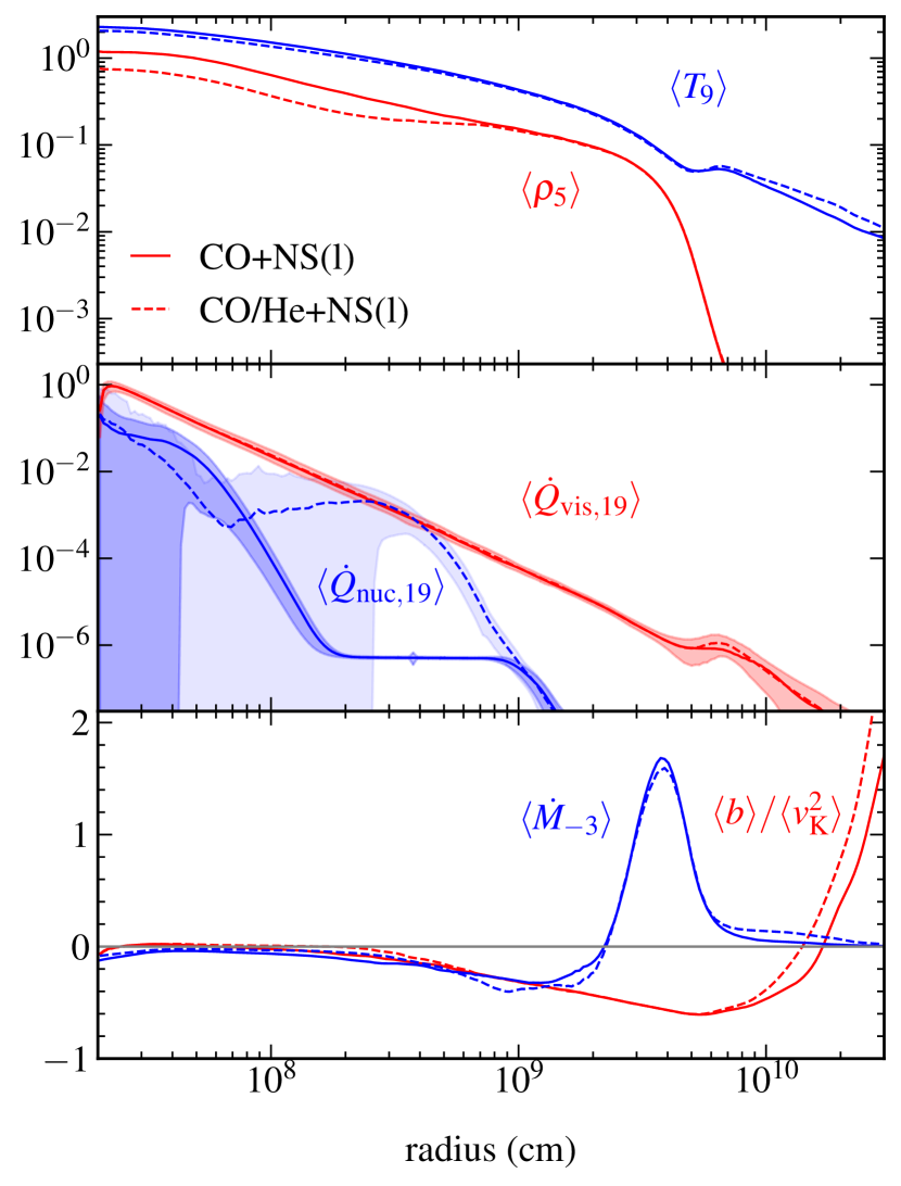
Figure 3: Time- and angle-averaged profiles of structural quantities for models CO+NS(l) and CO/He+NS(l) as a function of radius. The average is taken within $\pm 30^{\circ}$ of the equatorial plane, and within $\pm 60$ s (1.5 orbits at $r=R_{\rm t}$) of the time at which peak accretion is reached ($t\simeq 200$ s $\simeq$ 5 orbits). Quantities are defined as $\rho_{5}=\rho/(10^{5}\,\textrm{g\,cm}^{-3})$, $T_{9}=T/(10^{9}\,\textrm{K})$, $\dot{Q}_{\rm nuc,19}=\dot{Q}_{\rm nuc}/(10^{19}\,\textrm{erg\,[g\,s]}^{-1})$, $\dot{Q}_{\rm vis,19}=\dot{Q}_{\rm vis}/(10^{19}\,\textrm{erg\,[g\,s]}^{-1})$, and $\dot{M}_{-3}=\dot{M}/(10^{-3}\,M_{\odot}\textrm{s}^{-1})$. The average Keplerian speed $v_{\rm K}$ is given by equation (19), and the shaded areas in the middle panel bracket root-mean-square fluctuations (values for $\dot{Q}_{\rm vis}$ in model CO+NS(l) are not shown, for clarity).

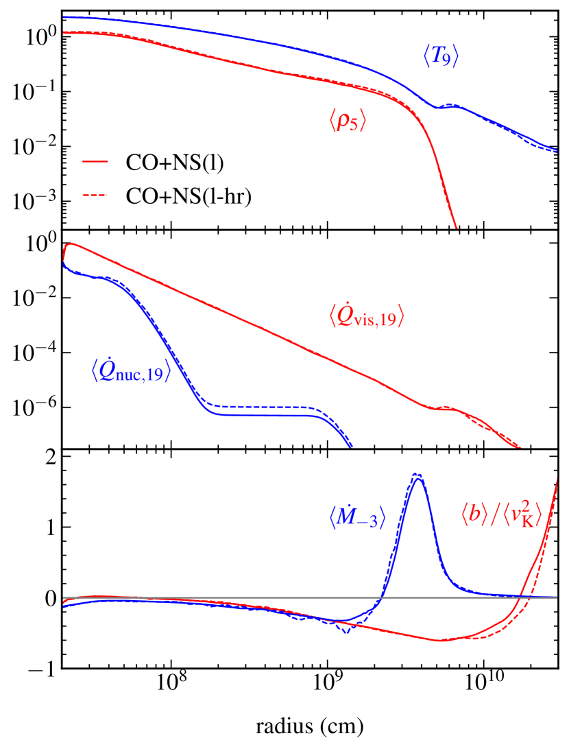
Figure 4: Same as Figure 3, but now comparing model CO+NS(l) with its high-resolution counterpart, CO+NS(l-hr). The structural profiles of the disk are essentially converged with resolution. The time-averaged profiles in the high-resolution model show more fluctuation because the data outputs were made at larger intervals in time, hence fewer snapshots are involved in the average for the same time period.

Figure 3 shows the average radial profiles of various quantities for the large inner boundary models CO+NS(l) and CO/He+NS(l), with the average taken within $30$ deg of the equatorial plane and within $3$ orbits at $r=R_{\rm t}$ from the time of peak accretion at the inner boundary $r=0.01R_{\rm t}$ ($206\pm 62$ s). The inner and outer portions of the disk which are respectively accreting and expanding are separated by the radius at which the accretion rate $\dot{M}=0$, and this radius moves outward in time. The temperature and density profiles vary slowly with radius in both models, with a slight decrease in the density profile for the hybrid WD model due to enhanced nuclear heating from He-burning reactions.

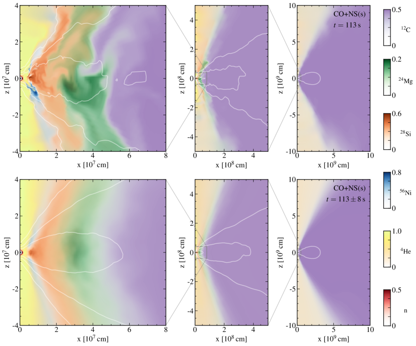
Figure 5: Snapshot of the default WD+NS merger model with small inner boundary [CO+NS(s)], which resolves accretion onto the neutron star. The top row shows the instantaneous mass fractions of various species, as labeled, at a time $t=113$ s ($2.7$ orbits at $r=R_{\rm t}$). The bottom row is a time average of snapshots in the range $105-121$ s. White contours correspond, from the inside out, to densities of {$10^{4}$, $3\times 10^{5}$, and $10^{5}$}g cm^-3, respectively. Panels on the left side are zoom-ins of panels on the right, as indicated by the gray lines.

In both models, the mean viscous heating dominates at all radii, except in the region where most of the He is burned in model CO/He+NS, where the mean nuclear heating rate is at most comparable to the average viscous heating. This additional nuclear heating is associated with an enhancement of $\sim 10\%$ in the ejected mass in this hybrid model (Table LABEL:t:results). While the fluctuations in the viscous heating term remain small over the entirety of the disk, nuclear burning becomes highly stochastic inside radii where heavier elements start to be produced. In the case of the hybrid model, these fluctuations can exceed the average viscous heating over a narrow range of radii, while for the fiducial model nuclear burning never dominates (the steep decrease of the viscous heating at small radii is an artifact of the boundary condition in the models shown in Figure 3). The relative weakness of nuclear burning helps explain why a thermonuclear runaway never takes place in our models.

Figure 3 also shows the profile of averaged Bernoulli parameter on the disk equatorial plane. This quantity adjusts to negative values close to zero at small radii. While the average Bernoulli parameter can be slightly positive near the inner boundary, this is a consequence of vertical alternations in sign in regions from which the outflow is launched. These average profiles of Bernoulli parameter are in broad agreement with the assumptions of Metzger (2012) and MM16.

Figure 4 compares average radial profiles in the fiducial WD+NS model and a version at twice the resolution in radius and angle. The profiles of all quantities are in excellent agreement except for nuclear burning around $r=R_{\rm t}$, which is slightly higher in the high-resolution model (but still sub-dominant relative to viscous heating). Table LABEL:t:results shows that the overall mass ejection is higher by about $10\%$ in the high-resolution model. While higher spatial resolution allows a better characterization of convective turbulence in the disk, the modest increase in mass ejection indicates that this convective activity is a sub-dominant factor in determining mass ejection compared to other processes such as viscous heating and angular momentum transport.

3.3 Evolution near the central object

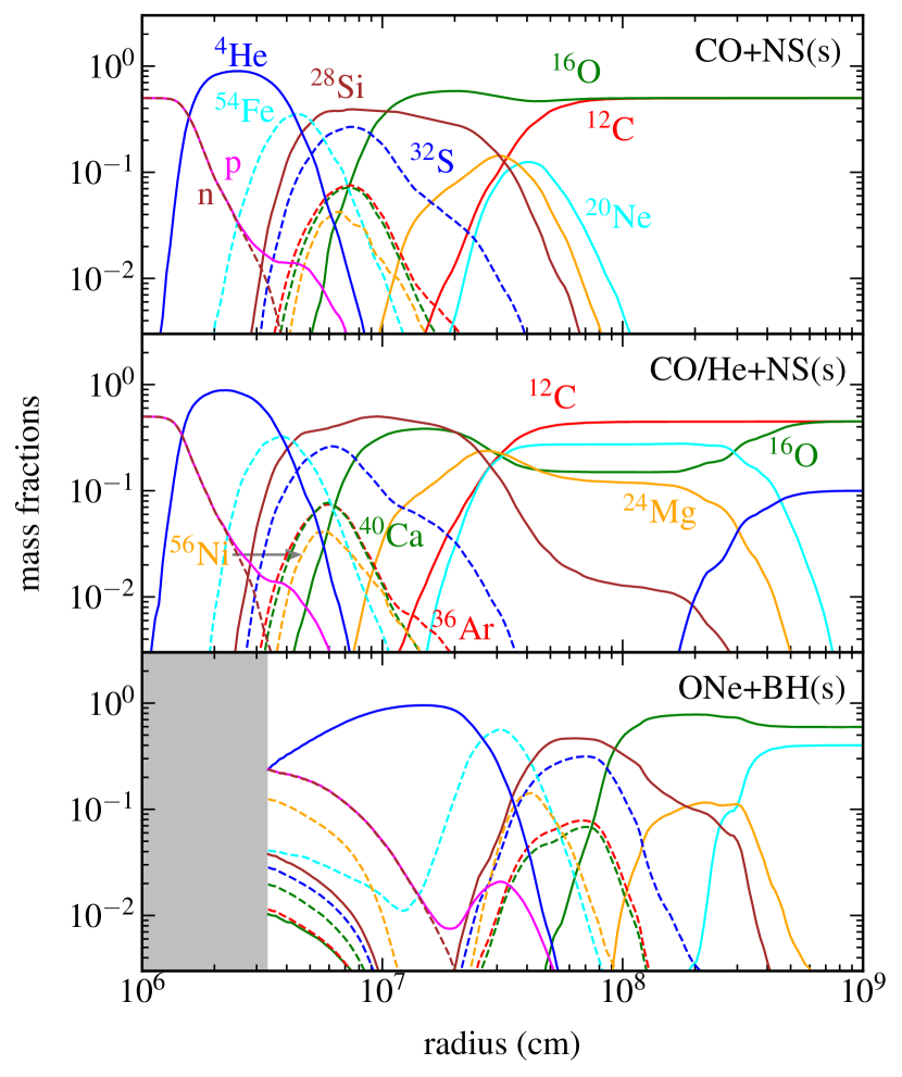
Figure 6: Time- and angle-averaged mass fractions of various species, as labeled, for small inner boundary models CO+NS(s) (top), CO/He+NS(s) (middle), and ONe+BH(s) (bottom), at $t=113\pm 3$ s ($2.8\pm 0.2$ orbits at $r=R_{\rm t}$) for the NS models and $t=39\pm 1.8$ s ($4.4\pm 0.2$ orbits at $r=R_{\rm t}$) for the BH model. The gray shaded area markes the inner boundary of the BH model, midway between the horizon and the ISCO.

A key property of disks formed in WD-NS/BH mergers is that nuclear fusion reactions of increasingly heavier elements take place as material accretes to smaller radii with higher temperatures and densities (Metzger, 2012). Our small inner boundary models can resolve this phenomenon in its entirety, at the expense of evolving for a short amount of time relative to $t_{\rm vis}$ given the more restrictive Courant condition at smaller radii.

None of our small-boundary models undergo a detonation. Given the deeper gravitational potential than in the large boundary models, nuclear energy release at these radii is less dynamically important, so this outcome is to be expected if detonations did not already occur at larger radii.

Figure 5 shows the spatial distribution of various species in our fiducial WD+NS model that resolves the compact object [CO+NS(s)]. Turbulence is associated with convection driven mostly by viscous heating but also by the nuclear energy released in fusion reactions. Species are launched from the same radii of the disk in which they are produced, with only moderate radial mixing. This stratification of mass ejection into different species becomes evident when taking a time-average of the flow (also shown in Figure 5), yielding a characteristic onion-shell-like structure as envisioned by Metzger (2012).

Time-averaged radial profiles of different abundances in the disk are shown in Figure 6 for the three baseline small boundary models. During accretion, elements that initially made up the WD are fused into heavier ones from the outside-in. The hybrid CO-He WD model shows a larger fraction of intermediate mass elements at larger radius than the fiducial CO WD, while the BH model completes all nucleosynthesis at larger radii due to the higher disk temperatures.

Given that we resolve the compact object, we are also able to resolve the radius inside which heavy elements undergo photodissociation into ⁴He nuclei and nucleons. In the vicinity of the NS surface, the composition is almost entirely neutrons and protons at the times shown. The BH model shows an increase in the heavy element abundance as the inner boundary is approached. This phenomenon is associated with a decreasing entropy given the net energy losses from nuclear reactions.

While the outflow composition is well stratified on spatial scales comparable to the disk thickness, as shown by Figure 5, significant mixing of the ejecta occurs as it expands outward, to the point where individual species are not distinguishable on scales comparable to the initial circularization radius $R_{\rm t}\sim 10^{9}$ cm. Note also that ejection of fusion products is confined to a narrow cone in angle $\lesssim 40$ deg from the rotation axis (Figure 7), which persists out to very large radii (Figure 5). Figure 7 suggests that nucleosynthesis products produced at deeper radii have narrower angular distributions around the rotation axis.

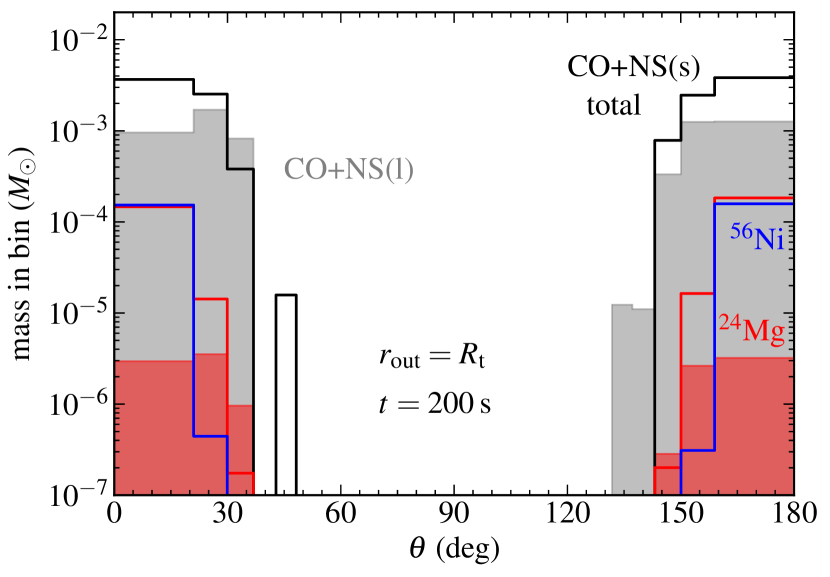
Figure 7: Mass histogram of unbound ejecta beyond $r=R_{\rm t}$ by $t=200$ s as a function of polar angle, for the default WD+NS model with small inner boundary [CO+NS(s), solid lines] and large inner boundary [CO+NS(l), shaded areas]. The black lines and gray shaded areas show total mass, while red and blue correspond to ²⁴Mg and ⁵⁶Ni only (the large boundary model does not make any ⁵⁶Ni).

To characterize the composition of outflows, we compute an average ejecta mass fraction for species $i$ as

$$\bar{X}_{i}(r_{\rm out},t_{\rm cmp})=\frac{\int dt\int d\Omega\,\rho v_{r}X_{i}}{\int dt\int d\Omega\,\rho v_{r}}$$ (21)

where the time integrals are carried out from the beginning of the simulation out to some fiducial comparison time $t_{\rm cmp}$, and the angular integral covers all polar angles. Table LABEL:t:results shows mass ejected and abundances for all models, measured at $r_{\rm out}=R_{\rm t}$ and by a time that allows to compare models with different durations ($170$ s for most NS models, and $30$ s for the BH models). The outflow from the fiducial small-boundary CO WD is dominated by ¹²C and ¹⁶O at a combined $\sim 80\%$ by mass, with all nucleosynthesis products contributing each at a few $\%$ level by mass. For the hybrid CO-He WD, the original WD elements are preserved at a combined $\sim 60\%$ by mass, with ²⁰Ne and ²⁴Mg being a significant secondary contribution at $21\%$ and $9\%$, respectively.

In the same way as with the large boundary models, the admixture of He in the fiducial CO WD results in more energetic nuclear burning and enhanced mass ejection. Table LABEL:t:results shows that when integrated out to the same time, the total unbound mass ejection within $r=R_{\rm t}$ is higher by $\sim 10\%$ in model CO/He+NS(s) than in CO+NS(s).

The outflow from the ONe WD + BH model is qualitatively different from the fiducial CO + NS case. The ejected mass is higher given the larger disk mass and a similar overall fraction ejected. Regarding composition, the initial WD material is preserved at a combined mass fraction of $66\%$, with ²⁸Si being the dominant nucleosynthetic product at $16\%$ by mass. While other products have abundances at a few $\%$ level by mass, a key property of this combination is the small amounts of ¹²C and ⁴He in the ejecta, at less than $0.1\%$ by mass.

In the fiducial and hybrid small boundary WD+NS models, the mass fraction of ⁵⁶Ni in the ejecta is $\sim 2\%$ at a time $170$ s. If we assume that this fraction remains constant in all ejecta and that the fraction of the disk mass is at least that estimated for the large boundary models ($0.4M_{\odot}$, which is a lower limit), we obtain a characteristic ⁵⁶Ni yield in the range $10^{-3}-10^{-2}M_{\odot}$. The non-spinning BH model with small boundary makes a larger fraction of ⁵⁶Ni which suggests a yield $\gtrsim 10^{-2}M_{\odot}$, given the larger WD mass and asymptotic ejected fraction. These estimates are optimistic, given the fact that burning fronts recede with time as the disk density decreases (MM16), implying that ⁵⁶Ni production will eventually stop. Most of the mass is ejected during peak accretion (Figure 8), however, and the ⁵⁶Ni fraction should remain approximately constant during this period. We thus expect that the late-time recession of the burning fronts will introduce corrections of order unity to the final ⁵⁶Ni yield. Our range of ejected ⁵⁶Ni is in agreement with previous estimates (Metzger 2012; MM16; Zenati et al. 2019).

No significant $r$-process production is expected in our models. Figure 6 shows that after photodissociation, the mass fractions of neutrons and protons remain equal all the way to the surface of the NS, thus preserving the initial $Y_{e}=0.5$ of the WD. While our models include charged-current weak interactions that modify $Y_{e}$, no appreciable neutronization occurs. At the surface of the NS we have $T\simeq 10^{10}$ K and $\rho\sim 10^{6}$ g cm^-3 (§3.4), for which electrons are trans-relativistic. The non-relativistic and relativistic Fermi energies are comparable and smaller than the thermal energy

$$\frac{p_{\rm F}^{2}}{2m_{e}kT} \simeq 0.2\rho_{6}^{2/3}T_{10}^{-1}$$ (22)

$$\frac{p_{\rm F}c}{kT} \simeq 0.5\rho_{6}^{1/3}T_{10}^{-1}$$ (23)

where $T_{10}=T/(10^{10}\,\textrm{K})$ and $\rho_{6}=\rho/(10^{6}\,\textrm{g}\,\textrm{cm}^{-3})$. Thus electrons are essentially non-degenerate, and the equilibrium electron fraction is close to $Y_{e}=0.5$. Even though neutrino cooling from electron-positron capture on nucleons is sub-dominant relative to other heating and cooling processes (§3.4), the timescale to change of $Y_{e}$ from charged-current weak interactions for non-degenerate material (e.g., Fernández et al. 2019)

$$\left(\frac{d\ln Y_{e}}{dt}\right)^{-1}\simeq 5T_{10}^{-5}\,\textrm{s}$$ (24)

is shorter than the characteristic evolutionary times. The lack of neutronization is thus a consequence of the non-degeneracy of the material. Whether these systems generate any $r$-process elements might depend on the details of angular momentum transport, which might result in higher accretion rates and densities at small radii, increasing the degeneracy of the material. This is not found for our choice of parameters.

3.3.1 Comparison of small- and large inner boundary models

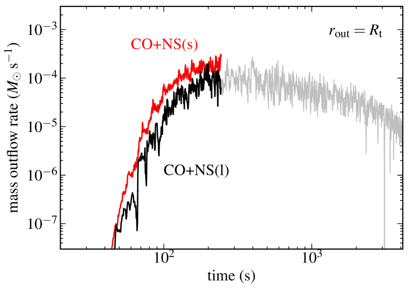
Figure 8: Unbound mass ejected at $r=R_{\rm t}$ as a function of time in the fiducial WD+NS models with large inner boundary (black and gray) and small inner boundary (red).

Given our approach to disk evolution that separates large- from small radius dynamics, it is important to make a connection between the two run types and to quantify the ejecta missing from the large boundary runs. Since the small boundary models cannot be evolved for nearly as long as large boundary runs, most of the ejecta from the former does not make it to a large enough radius to probe near-homologous expansion. Instead, we need to make the comparison at smaller radius, which we choose to be $r=R_{\rm t}$. By restricting the analysis to material with positive Bernoulli parameter, we separate bound disk material from unbound ejecta.

Figure 8 compares the mass outflow rate at $r=R_{\rm t}$ from the default WD+NS with small- and large inner boundary. As expected, the model that resolves the compact object ejects more mass (factor of $\sim 2$) than the large boundary model at all times up to the end of the simulation at $t=245$ s (Table LABEL:t:results). This time is in the range during which the mass accretion rate onto the compact object reaches its maximum value, evolving slowly with time before entering the power-law decay regime at around $t\simeq t_{\rm vis}$. The radial profiles of the ²⁰Ne and ⁵⁶Ni mass fractions as a function of time are shown in Figure 9, showing the location of the burning fronts. On a linear scale in time, these burning fronts are essentially at constant radii after $t\simeq 100$ s for this value of the viscosity parameter.

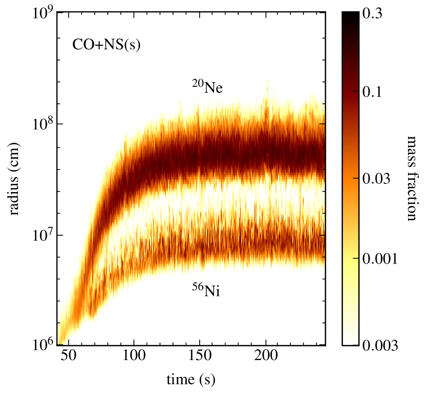
Figure 9: Radial profiles of the ²⁰Ne and ⁵⁶Ni mass fractions as a function of time for the fiducial WD+NS model with small inner boundary. See also Figure 6.

The angular distribution of material is very similar up to $t=200$ s, with both models ejecting the majority of the material within a funnel of $\lesssim 40$ deg from the rotation axis. The large boundary simulation does not show a significant difference between the angular distribution of the total ejecta (mostly C and O) and that of ²⁴Mg (the burning product with the largest mass fraction). In contrast, the small boundary model shows a trend in which burning products that are generated at smaller radii are ejected at narrower angles (on average) from the rotation axis. This is consistent with the snapshots in Figure 5, and suggests that despite the mixing, this angular segregation can persist to large radii.

The importance of resolving small radii is illustrated in Figure 10, which shows the velocity distribution of ejecta for both small- and large boundary fiducial WD+NS. The velocity distribution of the large boundary model cuts off at $v_{\rm max}\simeq\sqrt{GM_{c}/R_{\rm t}}\sim$ few $1,000$ km s^-1, which persists up to the end of the simulation (c.f., Figure 2). In contrast, the outflow from the small inner boundary model can reach maximum velocities that are about $10$ times higher. These velocities correspond to gravitational binding energies of radii as small as $0.01R_{\rm t}$, where nuclear energy release is still significant (Figures 6 and 9). Note also that the mean velocities of elements produced at smaller radii are higher: ¹²C is on average slower than ²⁴Mg (because it has more slow material), which in turn is slower than ⁵⁶Ni and ⁴He (the latter two have comparable distributions). This trend is consistent with the trend in the angular distribution of burning products.

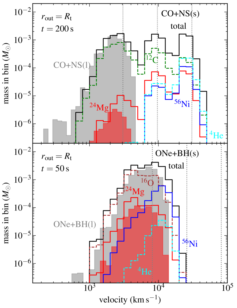
Figure 10: Mass histograms as a function of radial velocity, for unbound ejecta at $r=R_{\rm t}$ in the fiducial WD+NS models (top) and WD+BH models (bottom) at the times labeled, with solid lines denoting small-boundary versions and shaded areas their large-boundary counterparts. Black/grey histograms correspond to total ejecta, while green, brown, red, blue, and cyan histograms correspond respectively to ¹²C, ¹⁶O, ²⁴Mg, ⁵⁶Ni, and ⁴He. The vertical dashed lines correspond from left to right to the (point-mass) Keplerian velocity at radii $\{1,0.1,0.01\}R_{\rm t}$, respectively. Model CO+NS(s) uses a reflecting boundary condition at the surface of the NS, while all other models employ an outflow boundary condition at the smallest radius.

The marked difference between the small- and large-boundary velocity distribution for the fiducial WD+NS model is in part a consequence of the reflecting boundary condition at the NS surface for model CO+NS(s). The large boundary model has an outflow boundary condition, through which not only mass but also energy are lost. In contrast, the small boundary model is such that energy from accretion has nowhere to go except into a wind, given the weakness of neutrino and photodissociation cooling (§3.4). This difference stands in contrast to the large- and small-boundary BH models (also shown in Figure 10), both of which use an outflow inner radial boundary condition and have a velocity distribution that differs only by a factor of $\sim 2$ in their maximum velocity.

Finally, the composition of the outflow between large- and small boundary models is significantly different, as expected given the radii at which nucleosynthesis occurs. The fiducial large boundary model preserves the original WD composition at more than $99\%$ by mass, while this fraction drops to a combined $79\%$ (with different relative fractions) in the small boundary model. The large boundary hybrid CO-He WD model consumes a substantial fraction of the original ¹⁶O and ⁴He, yet it does not manage to make any significant ⁵⁶Ni. The large boundary BH model does make some ⁵⁶Ni, but the overall fractions of the heaviest elements are much smaller.

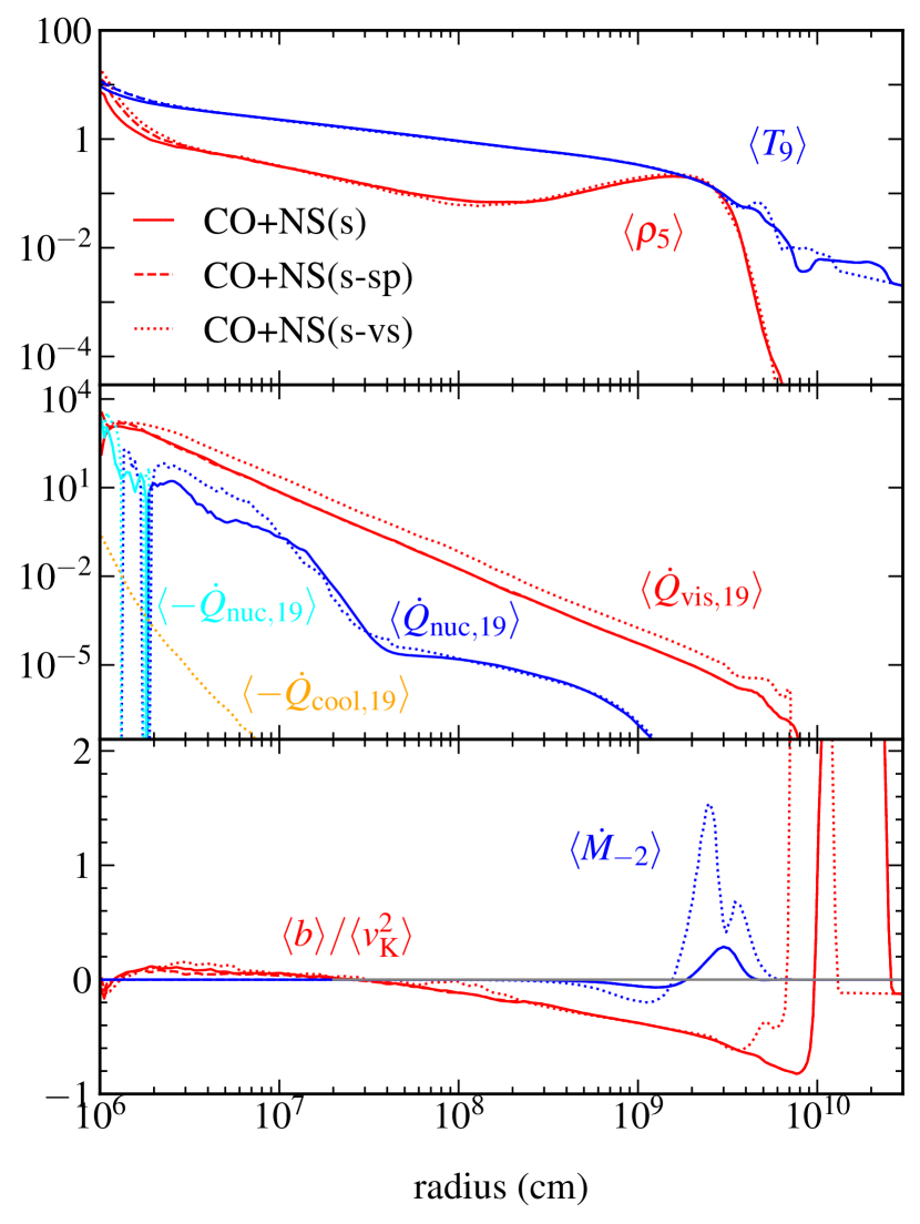
Figure 11: Time- and angle-averaged profiles of structural quantities for small inner boundary models with a NS, comparing the baseline model CO+NS(s), the model with a rotating NS CO+NS(s-sp) and a model with higher viscosity parameter CO+NS(s-vs). Quantities are the same as in Figure 3, and the time range for the average is $1.7\pm 0.2$ orbits at $r=R_{\rm t}$ ($70\pm 8$ s) for models CO+NS(s) and CO+NS(s-sp), and $0.5\pm 0.02$ orbits ($20.2\pm 0.8$ s) for model CO+NS(s-vs). Cyan curves show net energy loss from the nuclear reaction network due to photodissiation and thermal neutrino losses (not shown for model CO+NS(s-sp) for clarity, as it resembles that of CO+NS(s-vs)), and the orange curve show charged-current neutrino losses, shown only for model CO+NS(s-vs), for clarity.

3.4 Parameter dependencies

We now turn to addressing some of the parameter sensitivities of our results. Figure 11 shows time- and angle averaged profiles of various quantities for the baseline WD+NS model and variations of it with different viscosity parameter and spin of the neutron star. At a comparable evolutionary time, the model with higher viscosity differs in that (1) viscous heating is higher throughout the disk, (2) the disk evolution is faster, as indicated by the larger mass outflow rate at the disk outer edge, (3) nuclear energy release is a factor of a few larger inside $0.01R_{\rm t}$, and (4) the transition from positive to negative net energy generation by the reaction network moves inward in radius. The model with a spinning NS, evaluated at the same time as the baseline model, differs only inside $\sim 30$ km (3 NS radii), where a boundary layer develops. The additional viscous heating in this layer results in a somewhat higher temperature and an inward shift of the transition where neutrino cooling dominates over nuclear energy release, like in the high-viscosity model. In all three models, neutrino cooling from electron/positron capture onto nucleons is sub-dominant.

Figure 12 shows inner disk nucleosynthesis profiles for the three small boundary NS models. Abundances of all elements are very similar among models except within a few NS radii of the stellar surface, where the high-viscosity and spinning NS profiles both deviate from the baseline model in that photodissociation of ⁴He moves further out in radius given the higher temperatures. Table LABEL:t:results shows that the mass fractions in the outflow are very similar among all three models, with the possible exception of ¹²C and ⁴He, pointing to a robustness in the composition of the wind to the details of how angular momentum transport operates.

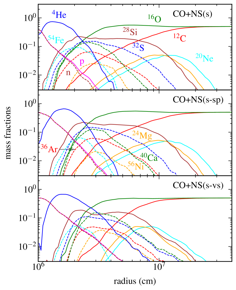
Figure 12: Time- and angle-averaged abundance profiles within $30$ deg of the equatorial plane over the same time period as in Figure 11, for the three small boundary models that resolve the NS surface [CO+NS(s), CO+NS(s-sp), and CO+NS(s-vs)]. Abundances have the same color coding as Figure 6.

The difference in profiles between the non-spinning and spinning BH models is shown in Figure 13. While the outer disk evolution is nearly identical, differences arise near the inner boundary, where the spinning BH model has slightly higher densities and temperatures. This bifurcation does not significantly affect the radius inside which photodissociation and thermal neutrino cooling dominate over nuclear heating, although net energy loss is stronger in the spinning BH model, even exceeding viscous heating near the inner boundary. Like the NS models, neutrino cooling due to charged-current weak interactions is negligible.

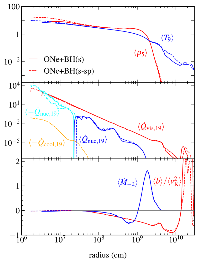
Figure 13: Same as Figure 11, but for the two small boundary models that resolve the BH: ONe+BH(s) (non-spinning) and ONe+BH(s-sp) (spin $\chi=0.8$). The time interval is $3\pm 0.3$ orbits at $r=R_{\rm t}$ ($26.6\pm 2.7$ s).

The nucleosynthesis profiles of the two BH models are shown in Figure 14. Differences become prominent inside the radius at which iron group nuclei start undergoing photodissociation into ⁴He and nucleons. At smaller radii, the spinning BH model has a lower abundance of heavy elements compared with the non-spinning case. Table LABEL:t:results shows however that the mass fractions in in the wind are very similar in those models, with the exception of ¹⁶O and ⁴He, indicating that radii close to the BH do not significantly contribute to the outflow.

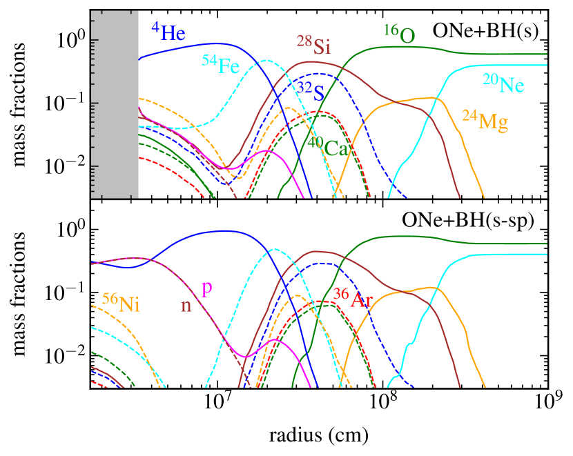
Figure 14: Same as Figure 12, but for the two small boundary models that resolve the BH. The time intervals are the same as for Figure 13.

3.5 Comparison with previous work

Our results are a significant improvement relative to Paper I. First, our new large boundary models, which cover a similar range as the simulations in Paper I, are evolved for a much longer time. Second, we also include more realistic microphysics, in particular an equation of state that accounts for radiation pressure, and a realistic nuclear reaction network. Finally, we can resolve the dynamics at the surface of the central object. The key qualitative difference with the results of Paper I is the absence of any detonation in our current models. Accretion proceeds in a quasi-steady way, with secular mass ejection on the viscous time of the disk.

Figure 15 compares instantaneous equatorial profiles of key quantities in the fiducial high-resolution model of Paper I (COq050_HR, used in Figures 1-3 of that paper) and in our high-resolution large-boundary WD+NS model CO+NS(l-hr), at a time shortly before a detonation occurs in the former. Both models employ the same equatorial resolution, domain size, torus parameters, central object mass, and boundary conditions. The model from Paper I assumes an ideal gas equation of state and point mass gravity, uses a different prescription for the viscosity (proportional to density, as in Stone et al. 1999), and uses a single power-law nuclear reaction calibrated to match ¹²C(¹²C,$\gamma$)²⁴Mg. While our new model evolves somewhat faster due to the different viscosity, the profiles of viscous heating differ by less than a factor of $2$. The key difference is the temperature profile, which differs by a factor $4$ at the radius where most of the nuclear burning occurs in the model of Paper I. The temperature profile in model CO+NS(l-hr) is shallower at small radius, which is a consequence of radiation pressure being dominant at this location, as shown in Figure 15. The burning rates correspondingly differ by several orders of magnitude.

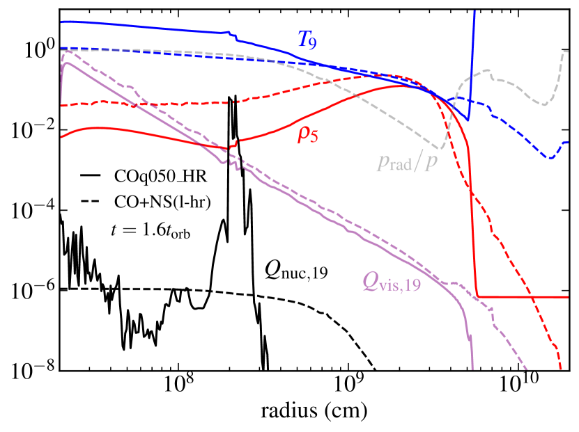
Figure 15: Instantaneous equatorial profiles of structural quantities at $t=1.6t_{\rm orb}$ in the fiducial high-resolution model of Paper I (COq050_HR, solid lines) and our fiducial high-resolution large boundary model (CO+NS(l-hr), dashed lines). The symbols have the same meaning as in Figure 3. The gray dashed curve shows the ratio of radiation to total pressure in model CO+NS(l-hr). The time is close to the onset of a detonation in model COq050_HR.

A separate question is whether detonations that should be occurring are not resolved in our current models. The mean accretion flow is such that burning fronts are spread out over distances comparable to the local radius (e.g., Figure 5), so no sudden releases of energy occur given that the radial accretion speed is subsonic. The turbulent r.m.s. Mach number around $r\sim 10^{8}$ cm is $\mathcal{M}_{\rm turb}\lesssim 0.3$ in model CO+NS(l-hr), which implies fractional temperature fluctuations of $\mathcal{M}_{\rm turb}/3\lesssim 10\%$ if radiation pressure dominates. Figure 3 shows that stochastic fluctuations in the burning rate are at most comparable to the viscous heating rate during peak accretion, when the density is the highest. The viscous heating timescale is itself a factor $\sim 10$ lower than the sound crossing time, thus nuclear burning is far from being able to increase the internal energy faster than the pressure can readjust the material. Settling the question of whether detonations occur during the initial establishment of the accretion flow to the central object will require simulations that employ magnetic fields to transport angular momentum and that fully resolve turbulence.

Zenati et al. (2019) carried out 2D hydrodynamic simulations starting from an equilibrium torus, and employing a nuclear reaction network, a realistic EOS, and self-gravity. They report weak detonations in all of their models excluding He WDs, followed by an outflow dominated by the initial WD composition, with an admixture of heavier elements. While we find the same type of outflow velocities and composition, our results differ in that we do not find any detonation in our models, weak or strong, even in the case of a hybrid CO-He WD with an admixture of He. This difference might be in part due to resolution, as their finest grid size (in cylindrical geometry) is 1 km. This is comparable to the resolution of our models at $r=10^{7}$ cm, but coarser in the vicinity of the NS (our grid is logarithmic in radius, and on the midplane we have $\Delta r/r\simeq 0.037\simeq\Delta\theta\simeq 2^{\circ}$). Our results are consistent with those of Fryer et al. (1999), which found that nuclear burning was energetically unimportant during disk formation.

The time-averaged profiles in the disk equatorial plane show very close similarity to the 1D results of Metzger (2012) and MM16. Figure 16 shows the profile of absolute value of the radial mass flow rate for the fiducial and hybrid small boundary models. A power-law fit to the radial dependence of the accretion rate $\dot{M}\propto r^{p}$ yields $p\simeq 0.7$ except in the vicinity of the NS and where the disk has not yet reached steady accretion. In the mass-loss model of MM16, this corresponds to disk outflow velocities comparable to the local Keplerian speed $v_{\rm K}$. This is consistent with the velocity distribution of the outflow (Figure 10), which shows an upper limit comparable to the Keplerian speed at the innermost radius where ⁵⁶Ni is produced (Figure 9). We also find a characteristic power-law decline of the outflow rate with time after peak accretion has been achieved (Figure 2). The radial dependence of the mass fractions is remarkably similar to that of MM16 (c.f. their Figure 5), although the radial position of our burning fronts evolves more slowly (compare our Figure 9 with their Figure 6). This is a consequence of our fiducial model using a lower viscosity parameter ($0.03$) than their fiducial case ($0.1$).

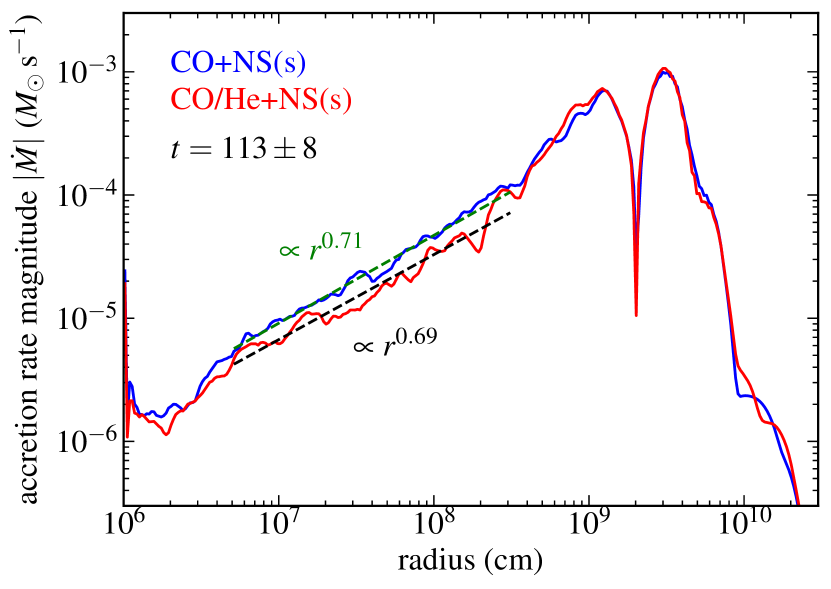
Figure 16: Time- and angle-averaged mass flow rate (absolute value) for the fiducial small boundary WD+NS model and its hybrid counterpart. The angle-average is taken within $30$ deg of the equatorial plane. The dashed lines show power-law fits to the radial dependence of the accretion rate.

4 Observational Implications

The outflow from the accretion disk should generate an electromagnetic transient that rises over a few day timescale and reaches a peak luminosity $\sim 10^{40}$ erg s^-1 if powered only by radioactive decay. We can estimate this rise time and peak luminosity from the velocity distribution of ejected ⁵⁶Ni and our estimate of the total ejecta from the disk (equation 16, Table LABEL:t:results).

Figure 17 shows the velocity distribution of ejected ⁵⁶Ni at various times in the fiducial small-boundary WD+NS model, measured at the initial torus radius, which is $\sim 100$ times larger than the radius at which ⁵⁶Ni is produced (Figure 9). The average velocity decreases as a function of time, which means that on average, faster material is ejected before slower material and therefore resides at larger radii, even if mixing takes place. Ignoring corrections due to the geometric collimation of the outflow, this stratification in radius and velocity means that radiation escapes from faster layers first. In our estimates, we therefore consider the cumulative mass starting from the highest velocity,

$$M_{i}(>v)=\int_{v}^{v_{\rm max}}\frac{dM_{i}}{dv}\,dv.$$ (25)

where the subscript $i$ stands for either total mass or ⁵⁶Ni mass. Note that this is a lower limit on the velocity, since thermal energy can be converted to kinetic via adiabatic expansion.

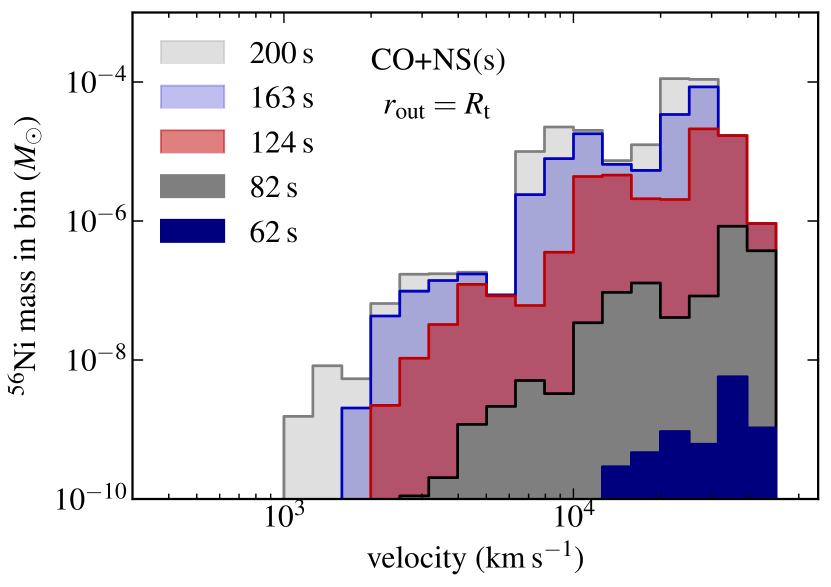
Figure 17: Mass histograms of unbound ⁵⁶Ni as a function of radial velocity for model CO+NS(s), measured at $r_{\rm out}=R_{t}$ and at the labeled times.

The time for radiation to escape from a layer with total mass $M_{\rm tot}(>v)$ is given by (Arnett, 1979)

$$t_{\rm pk}(>v)=\left[\frac{3\kappa M_{\rm tot}(>v)}{4\pi cv}\right]^{1/2}.$$ (26)

In evaluating equation (26), we adopt $\kappa=0.05$ g cm^-3 for a Fe-poor mixture (MM16), and obtain $M_{\rm tot}(>v)$ by renormalizing the ⁵⁶Ni mass distribution by a conservative total ejecta mass of $0.4M_{\odot}$ (Table LABEL:t:results). To estimate uncertainties, we also compute this mass by re-normalizing the total (not just ⁵⁶Ni) velocity distribution to the same total ejected mass.

The luminosity of a layer with ⁵⁶Ni mass $M_{\rm Ni}(>v)$ at time $t=t_{\rm pk}(>v)$ is

$$L_{\rm pk}(>v) = M_{\rm Ni}(>v)\left[\dot{Q}_{\rm Ni}(t_{\rm pk})+\dot{Q}_{\rm Co}(t_{\rm pk})\right]$$ (27)

where the specific nuclear heating rates from ⁵⁶Ni and ⁵⁶Co decay are

$$\dot{Q}_{\rm Ni}(t) = \frac{\Delta E_{\rm Ni}}{m_{\rm Ni}\tau_{\rm Ni}}\,e^{-t/\tau_{\rm Ni}}$$ (28)

$$\simeq 4.8\times 10^{10}\textrm{\,[erg\,g}^{-1}\textrm{\,s}^{-1}]\,e^{-t/\tau_{\rm Ni}}$$

$$\dot{Q}_{\rm Co}(t) = \frac{\Delta E_{\rm Co}}{m_{\rm Co}}\frac{(\tau_{\rm Ni}\tau_{\rm Co})^{-1}}{(1/\tau_{\rm Ni}-1/\tau_{\rm Co})}$$

$$\simeq 8.9\times 10^{9}\textrm{\,[erg\,g}^{-1}\textrm{\,s}^{-1}]\,\left(e^{-t_{\rm pk}/\tau_{\rm Co}}-e^{-t_{\rm pk}/\tau_{\rm Ni}}\right),$$

with $\left\{\tau_{\rm Ni},\tau_{\rm Co}\right\}\simeq\left\{8.8,111\right\}$ d the mean lifetimes and $\left\{\Delta E_{\rm Ni},\Delta E_{\rm Co}\right\}\simeq\left\{2.1,4,6\right\}$ MeV the decay energies of ⁵⁶Ni and ⁵⁶Co, respectively. Equation (27) assumes that the gamma-rays from radioactive decay are thermalized with $100\%$ efficiency. The total ⁵⁶Ni mass is obtained by scaling the ejected distribution to a (conservative) estimate of $10^{-3}M_{\odot}$, which is somewhat smaller than the ejected fraction times total ejected mass for this model (Table LABEL:t:results).

Figure 18 shows $t_{\rm pk}(>v)$ and $L_{\rm pk}(>v)$ as a function of outflow velocity for the fiducial small-boundary WD+NS model. The rise time to peak from half maximum is in the range $2-3$ d depending on whether the ⁵⁶Ni or total velocity distributions are used, and the rise time to the mass-averaged velocity is the same. The peak luminosity is a few times $10^{40}$ erg s^-1. This value can increase by a factor $10$ if the ⁵⁶Ni yield is on the higher end of our estimates, $10^{-2}M_{\odot}$, coming closer to normal supernova luminosities. A rough approximation to the light curve can be obtained by plotting $L_{\rm pk}(>v)$ versus $t_{\rm pk}(>v)$, which is shown in Figure 19.

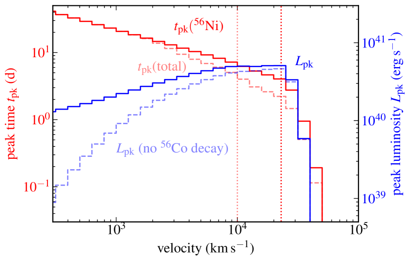
Figure 18: Time to reach peak emission (equation 26, red) and peak luminosity (equation 27, blue) for material with velocity larger than a given value (equation 25) in model CO+NS(s). Solid red shows $t_{\rm pk}$ computed using the ⁵⁶Ni velocity distribution at $t=200$ s (Figure 17) renormalized to $0.4M_{\odot}$, while the dashed red line shows the same calculation but with the (renormalized) total velocity distribution. The vertical dotted lines show the corresponding mass-weighted average velocities. The dashed blue line shows $L_{\rm pk}$ without the contribution from ⁵⁶Co heating in equation (27). For the peak luminosity, we assume an initial ⁵⁶Ni mass of $10^{-3}M_{\odot}$.

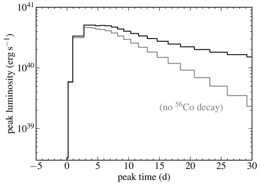
Figure 19: Peak luminosity (equation 27) as a function of peak time (equation 26) for material with velocity larger than a given value (equation 25) for model CO+NS(s). This is a rough approximation to the light curve of the radioactively-powered transient expected from the disk outflow. The reverse-cumulative mass distribution for the peak time is obtained by integrating the ⁵⁶Ni mass distribution (Figure 17) and re-normalizing by the asymptotic total mass ejected ($\sim 0.4M_{\odot}$), while the luminosity is obtained by renormalizing the distribution to $10^{-3}M_{\odot}$ of ⁵⁶Ni. The gray line shows the peak luminosity without the contribution of ⁵⁶Co to estimate the uncertainty range from our assumption of complete gamma-ray thermalization.

The short rise time suggests a connection to previously found rapidly-evolving blue transients (e.g., Drout et al. 2014; Rest et al. 2018; Chen et al. 2019) but with much lower luminosities. It is possible that the ejecta from the disk collides with material previously ejected in a stellar wind by one or both of the progenitors of the WD and/or NS/BH, resulting in enhanced emission relative to our simple estimates based on radioactive heating. Another way to enhance the luminosity above that from radioactive decay is through accretion power (e.g., Dexter & Kasen 2013, MM16). Extrapolating the accretion rate in Figure 1 for model CO+NS(s) to $t\simeq t_{\rm peak}\simeq 3$ d, yields $\sim 10^{43}$ erg s^-1 for a $10\%$ thermalization efficiency.

In addition to powering a supernova-like transient from the unbound ejecta, we speculate that the inner parts of the accretion flow (near the central NS or BH) could generate a relativistic jet similar to those in gamma-ray bursts (e.g., Fryer et al. 1999; King et al. 2007). We obtain peak accretion rates onto the central compact object of $\sim 10^{-6}-10^{-3}M_{\odot}$ s^-1, with a peak timescale of tens to hundreds of seconds (Figure 1). Assuming a jet launching efficiency of $\epsilon_{\rm j}\lesssim 0.1$, the peak jet power could therefore be $\epsilon_{j}\dot{M}c^{2}\lesssim 10^{47}-10^{50}$ erg s^-1. While these characteristic luminosities (timescales) are somewhat too low (long) compared to the majority of long-duration gamma-ray bursts, they may be compatible with other high energy transients. For instance, Xue et al. (2019) recently discovered an X-ray transient, CDF-S XT2, with Chandra with a peak isotropic luminosity $L_{\rm X}\sim 3\times 10^{45}$ erg s^-1 and peak duration $\sim 10^{3}$ s. The late-time decay of the X-ray luminosity, with a time exponent $2.16^{+26}_{-29}$, is in broad agreement with the decay rate of the accretion rate in our models (Figure 1). While peak accretion in our models occurs somewhat earlier, this peak time is tied to how angular momentum transport is modeled. The host galaxy and spatial offset of CDF-S XT2 from its host, while consistent with those of NS-NS mergers, would plausibly also be consistent with the older stellar populations that can host WD-NS/BH mergers.

WD-NS mergers have also been discussed as a possible formation channel of pulsar planets (Phinney & Hansen, 1993; Podsiadlowski, 1993; Margalit & Metzger, 2017). Using a semi-analytic model extending the torus evolution to $\sim$kyr post merger, Margalit & Metzger (2017) found that conditions conducive to formation of planetary bodies consistent with the B1257+12 pulsar planets (Wolszczan & Frail, 1992; Wolszczan, 1994; Konacki & Wolszczan, 2003) can be achieved for sufficiently low values of the alpha viscosity parameter $\alpha$ and accretion exponent $p$. The index of $p\sim 0.7$ we find in our current work (Figure 16) is somewhat higher than that required to obtain significant mass at the location of the planets and to spin-up the NS to millisecond periods, however this is subject to several uncertainties. Simulations of radiatively-inefficient accretion disks typically find $p\sim 0.4-0.8$ depending on the physics (hydrodynamic vs MHD simulations), the value of the alpha viscosity parameter, and the initial magnetic field (e.g. Yuan et al., 2012; Yuan & Narayan, 2014), while observations of Sgr A* suggest even lower values, $p\sim 0.3$ (Yuan & Narayan, 2014) (although the physical accretion regime of Sgr A* is very different than the WD-NS merger accretion disks considered here). Whether or not some of the matter expelled from the disk midplane remains bound and eventually circulates back is also not entirely resolved and can increase the remaining disk mass at late times, increasing the viability of the WD-NS merger pulsar-planet formation scenario.

5 Summary and Discussion

We have carried out two-dimensional axisymmetric, time-dependent simulations of accretion disks formed during the (quasi-circular) merger of a CO or ONe WD by a NS or BH. Our models include a physical equation of state, viscous angular momentum transport, self-gravity, and a coupled $19$-isotope nuclear reaction network. We studied both the long-term mass ejection from the disk, by excluding the innermost regions, and fully global models that resolve the compact object but which can only be evolved for shorter than the viscous timescale of the disk. Our main results are the following:

1. In all of the models we study, accretion and mass ejection proceed in a quasi-steady manner on the viscous time, with no detonations. Nuclear energy generation is at most comparable to viscous heating (Figures 3, 4, 11, and 13).

2. The radiatively-inefficient character of the disk results in vigorous outflows. At least $50\%$ of the initial torus should be ejected in the wind (Figure 2 and Table LABEL:t:results). The velocity distribution of this outflow is broad, covering the range $10^{2}-10^{4}$ km s^-1 (Figures 2 and 10). The outflow is concentrated within a cone of $\sim 40$ deg from the rotation axis (Figure 2 and 7). Energy losses due to photodissociation and thermal neutrino emission become important only near the central compact object, with neutrino emission from electron/positron capture onto nucleons being sub-dominant (Figure 11 and 13).

3. Our models can capture the burning of increasingly heavier elements, as accretion proceeds to large radii, all the way to the iron group elements and its subsequent photodissociation into ⁴He and nucleons (Figures 5, 6, 12 and 14). The outflow composition is dominated by that of the initial WD, with burning products accounting for $10-30\%$ by mass (Table LABEL:t:results). Based on the mass fractions of elements in the wind and the ejecta masses from large boundary models, we estimate that $10^{-3}-10^{-2}M_{\odot}$ of ⁵⁶Ni should be produced generically by these disk outflows. The wind composition is relatively robust to variations in the disk viscosity, rotation rate of the NS or BH, and spatial resolution. No significant neutronization (and thus $r$-process production) is expected from our models.

4. Two predictions from our results are that (1) the average velocities of burning products generated at smaller radii are higher (i.e., helium and iron should be faster on average that Mg or Si; Figure 10), and that (2) these burning products should be (on average) concentrated closer to the rotation axis than lighter elements (Figure 7).

5. Based on the ejecta mass and velocity, we estimate that the resulting transients should rise to their peak brightness within a few days (Figures 18). When including only heating due to radioactive decay of ⁵⁶Ni (and ⁵⁶Co) generated in the outflow, we obtain peak bolometric luminosities in the range $\sim 10^{40}-10^{41}$ erg s^-1. This luminosity can be enhanced by circumstellar interaction or late-time accretion onto the central object (Figure 1), potentially accounting for the properties of rapidly-evolving blue transients (§4). The generation of a relativistic jet by accretion onto the central object could also account for X-ray transients such as CDF-S XT2.

The main improvement to be made in our models is the replacement of a viscous stress tensor for full magnetohydrodyanmic (MHD) modeling. Comparison between hydrodynamic and MHD models (with initial poloidal geometry) of accretion disk from NS-NS/BH mergers shows close similarity in the ejection properties of the thermal outflows in the radiatively-inefficient phase; this thermal component is the entirety of the wind in hydrodynamics, but only a subset of the ejection when MHD is included (Fernández et al., 2019). While in principle such magnetized disks can generate jets, the disruption of the WD will leave a significant amount of material along the rotation axis, which can pose difficulties for launching relativistic outflows.

The second possible improvement is using realistic initial conditions obtained from a self-consistent simulation of unstable Roche lobe overflow. Since the thermodynamics of the disk become quickly dominated by heating from angular momentum transport and nuclear reactions, it is not expected that the details of the initial disk thermodynamics will have much incidence on the subsequent dynamics except if (1) nuclear burning becomes important during the disruption process itself, as expected for a ONe WD merging with a NS (e.g., Metzger 2012) or (2) if the magnetic field configuration post merger (which should be mostly toroidal, in analogy with NS-NS mergers) generates significant deviations from the evolution obtained with viscous hydrodynamics.

The evolution of disks from He WDs around NS or BHs is expected to be more sensitive to the choice of parameters such as the disk entropy, mass, and viscosity parameter (MM16). We therefore leave simulations of such systems for future work.

Appendix A Implementation of Self-Gravity

We implement self-gravity in spherical coordinates using the multipole algorithm of Müller & Steinmetz (1995). While FLASH3 includes a version of this algorithm, it is not optimized for non-uniform axisymmetric spherical grids. Here we provide a brief description of our customized implementation and tests of it.

The truncated multipole expansion of the gravitational potential $\Phi$ in axisymmetry is

$$\Phi(r,\theta)=-2\pi G\sum_{\ell=0}^{\ell_{\rm max}}\,P_{\ell}(\cos\theta)\left[\frac{1}{r^{\ell+1}}C_{\ell}(r)+r^{\ell}D_{\ell}(r)\right],$$ (30)

where $P_{\ell}$ is the Legendre polynomial of index $\ell$, and the radial density moments are given by

$$C_{\ell}(r) = \int_{0}^{\pi}\sin\theta d\theta P_{\ell}(\cos\theta)\int_{0}^{r}dR\,R^{2+\ell}\rho(R,\theta)$$ (31)

$$D_{\ell}(r) = \int_{0}^{\pi}\sin\theta d\theta P_{\ell}(\cos\theta)\int_{r}^{\infty}dR\,R^{1-\ell}\rho(R,\theta).$$ (32)

Equation (30) is an exact solution of Poisson’s equation (equation 6) when $\ell_{\rm max}\to\infty$. In practice, the sum needs to be truncated at some finite $\ell_{\rm max}$, the optimal value of which is problem-dependent (Müller & Steinmetz, 1995). The main computational work involves calculation of the moments $C_{\ell}(r)$ and $D_{\ell}(r)$.

In the Müller & Steinmetz (1995) algorithm, the integrals in equations (31)-(32) are first replaced by sums of integrals inside each computational cell. One then assumes that the density varies smoothly within a cell, thus decoupling the angular integral of Legendre polynomials, the radial integral of the weight, and the density. The angular integral can be calculated exactly from recursion relations of these polynomials, while the radial integral can be solved analytically. For a cell with indices $(i,j)$, the moments are thus

$$C^{ij}_{\ell} = \sum_{q=i}^{i_{\rm max}}\sum_{j=1}^{j_{\rm max}}\left[\int_{\theta_{j-1/2}}^{\theta_{j+1/2}}\sin\theta d\theta P_{\ell}(\cos\theta)\right]$$ (33)

$$\qquad\times\,\frac{\rho_{ij}}{3+\ell}\left(r_{q+1/2}^{3+\ell}-r_{q-1/2}^{3+\ell}\right)$$

$$D^{ij}_{\ell} = \sum_{q=1}^{i}\sum_{j=1}^{j_{\rm max}}\left[\int_{\theta_{j-1/2}}^{\theta_{j+1/2}}\sin\theta d\theta P_{\ell}(\cos\theta)\right]$$ (36)

$$\times\rho_{ij}\left\{\begin{array}[]{l}\left(r_{q+1/2}^{2-\ell}-r_{q-1/2}^{2-\ell}\right)/(2-\ell)\quad(\ell\neq 2)\\ \vskip 3.0pt plus 1.0pt minus 1.0pt\cr\ln{\left(r_{q+1/2}/r_{q-1/2}\right)}\qquad\qquad\phantom{a}(\ell=2)\end{array}\right.$$

where half-integer indices denote cell edges, and $\rho_{ij}$ is the volume-averaged density of the cell.

The angular and radial integrals are computed once at the beginning of the simulation. To improve accuracy, Müller & Steinmetz (1995) recommend computing the sum in equation (33) from small radii to large radii, and vice-versa for equation (36). In practice, in our non-uniform grid implementation, the domain is spatially decomposed by compute core. The sums are first computed locally within each core, and then each core broadcasts the total of the sum within itself to the others. Finally, global cumulative sums are constructed locally with the information from all other cores. The final gravitational potential is computed by adding the contribution of the point mass from the neutron star (equation 6). Overall, the gravity solver ads a cost of approximately $50\%$ that of the hydrodynamic solver. The latter is comparable or smaller than the cost of the nuclear reaction network, therefore the inclusion of self-gravity is only a moderate addition to the computational budget.

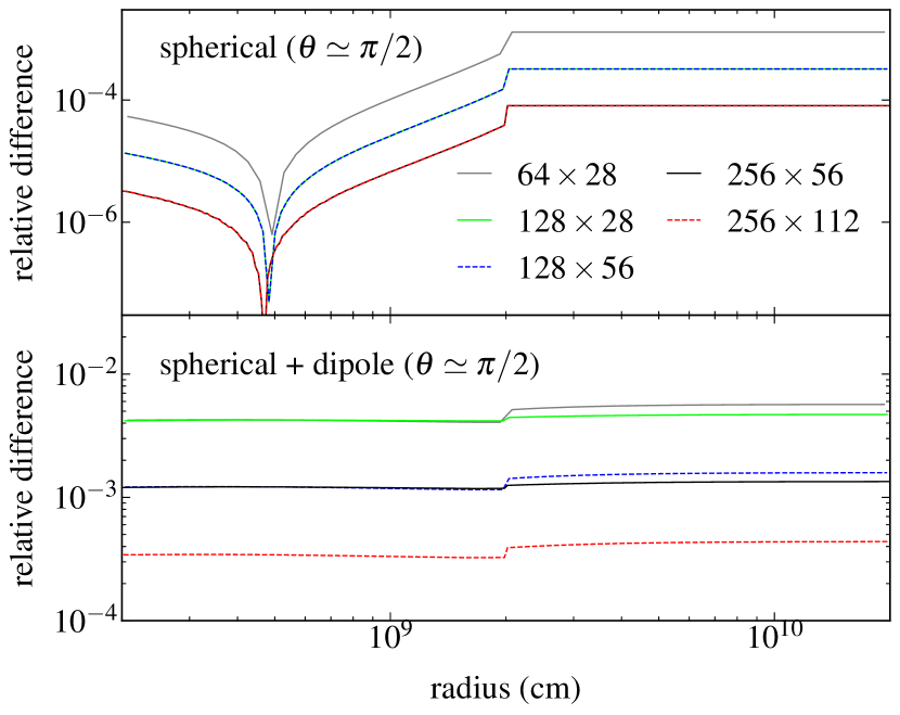
Figure 20: Numerical test of the multipole solver. Shown as a function of radius is the fractional difference between the numerical solution and the analytic potential in equation (38), when initializing the domain with the density profile of equation (37). The top panel restricts the density profile to the spherical component only ($P_{2}=0$), while the bottom panel uses both spherical and dipolar components (the multipole solver allows $\ell\leq\ell_{\rm max}=12$). The resolutions shown correspond to grids logarithmically spaced in radius and equispaced in $\cos\theta$, extending over the full range of polar angles, and an inner boundary at $r_{\rm in}=2\times 10^{8}$ cm and an outer boundary $100$ times larger. The parameters of the analytic solution are $\rho_{0}=10^{7}$ g cm^-3 and $R=2\times 10^{8}$ cm. Curves are computed for a single angular direction (cell center adjacent to equatorial plane from above).

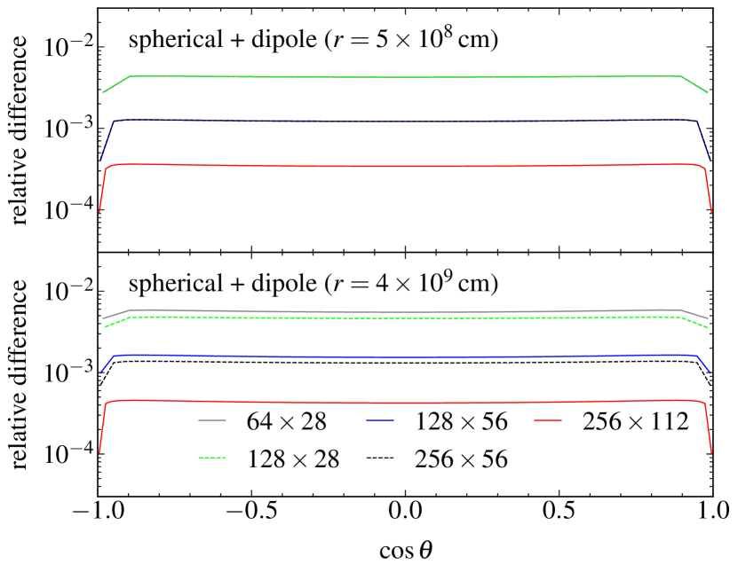
Figure 21: Same as Figure 20, but showing results as a function of polar angle when including both spherical and dipolar components. Top and bottom panels use radii in the interior ($r\leq R$) and exterior ($r>R$) parts of the solution, respectively.

We test our implementation by comparing it against an analytic solution. Using the density profile

$$\rho(r,\theta)=\bigg{\{}\begin{array}[]{lr}\rho_{0}\left[1+P_{2}(\cos\theta)\right]&r\leq R\\ \vskip 3.0pt plus 1.0pt minus 1.0pt\cr 0&r>R\end{array}$$ (37)

with $\rho_{0}$ and $R$ constant, yields the following gravitational potential:

$$\Phi=-2\pi G\rho_{0}\left[I_{0}(r)+I_{2}(r)P_{2}(\cos\theta)\right]$$ (38)

with

$$I_{0}(r) = \bigg{\{}\begin{array}[]{lr}(2/3)(r^{3}-r_{\rm in}^{3})/r+(R^{2}-r^{2})&r\leq R\\ \vskip 3.0pt plus 1.0pt minus 1.0pt\cr(2/3)(R^{3}-r_{\rm in}^{3})/r&r>R\end{array}$$ (41)

$$I_{2}(r) = \frac{2}{5}\bigg{\{}\begin{array}[]{lr}(r^{5}-r_{\rm in}^{5})/(5r^{3})+r^{2}\ln(R/r)&r\leq R\\ \vskip 3.0pt plus 1.0pt minus 1.0pt\cr(R^{5}-r_{\rm in}^{5})/(5r^{3})&r>R\end{array}$$ (44)

where $r_{\rm in}$ corresponds to the inner radial boundary.

For our tests, we use a computational domain extending from $r_{\rm in}=2\times 10^{8}$ cm to a radius $100$ times larger, covering all polar angles ($\theta\in[0,\pi]$). The density normalization and transition radius are $\rho_{0}=10^{7}$ g cm^-3 and $R=2\times 10^{8}$ cm, respectively. The multipole solver is run with $\ell_{\rm max}=12$. The grid sizes used are $64\times 28$, $128\times 28$, $128\times 56$, $256\times 56$, and $256\times 112$ in radius and polar angle (logarithmic, and equispaced in $\cos\theta$, respectively). Figure 20 shows the fractional difference between the potential obtained from the multipole solver and that in the analytic solution. In all cases, increasing the spatial resolution brings the numerical value closer to the analytic solution. Agreement is better when restricting the density profile to be spherical only ($P_{2}=0$ in equations 37 and 38) than when using both spherical and dipole components. Note that agreement requires all other moments (up to $\ell_{\rm max}=12$) to have vanishing amplitudes.

At our standard resolution ($128\times 56$), agreement is of the order of $10^{-3}$, with a very weak radial dependence. The small bump at $r=R$ coincides with the transition from interior to exterior solution in equation 38. Figure 21 also shows that the fractional deviation is mostly uniform with polar angle, both in the interior and exterior regions. The accuracy of the $\ell=0$ moment is determined by the radial resolution only, while the angular resolution becomes more important when adding the dipole component, with smaller changes introduced by the radial resolution.

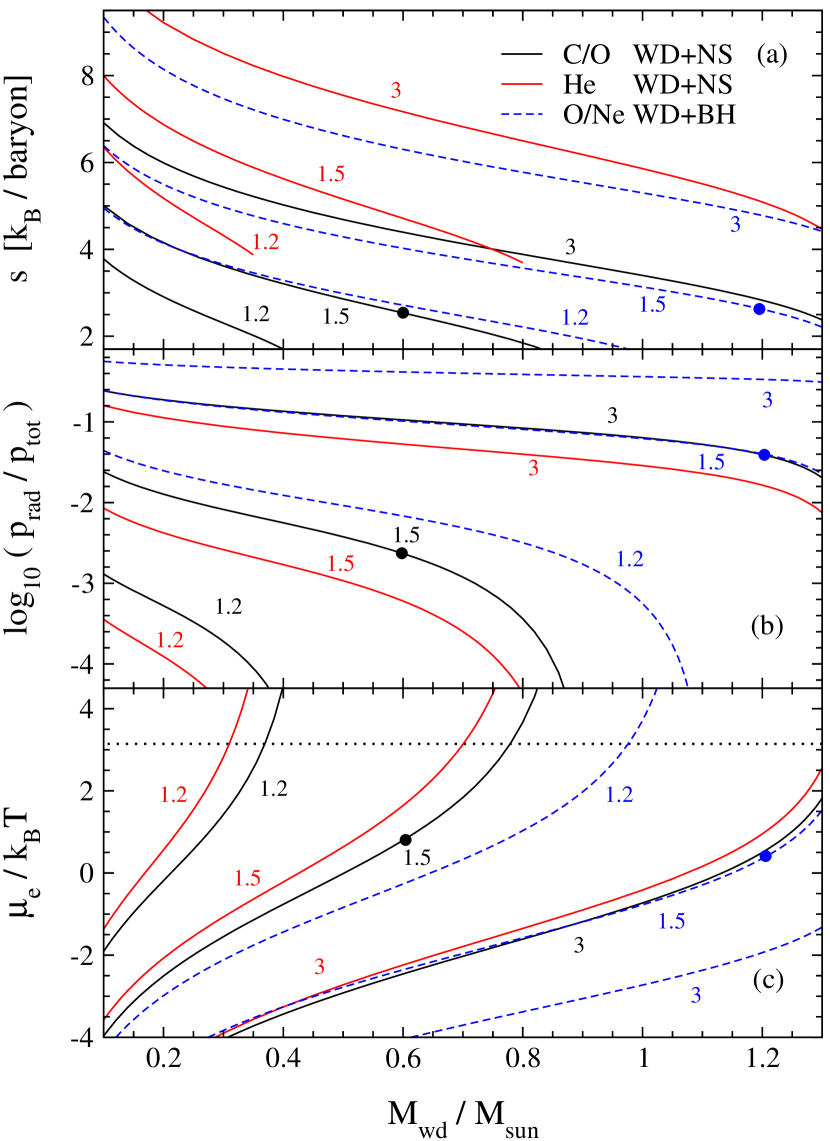
Figure 22: Properties of equilibrium tori constructed with the Helmholtz equation of state and point mass gravity, as a function of disk (WD) mass. Shown are (a) entropy, (b) ratio of radiation to total pressure at density maximum, and (c) degeneracy parameter at density maximum. Each curve is labeled by the value of the torus distortion parameter (eq. [45]). For reference, $d=\{1.2,1.5,3\}$ correspond to $e_{\rm int}/(GM_{\rm c}/R_{0})\simeq\{5\%,10\%,20\%\}$ at pressure maximum, respectively, and to $H/R_{0}\sim\{0.4,0.6,1\}$, respectively. Solid and dashed lines correspond to $M_{\rm c}=1.4M_{\odot}$ and $M_{\rm c}=5M_{\odot}$, respectively. Colors label the composition: $\{X_{\rm C}=X_{\rm O}=0.5\}$ (black), $X_{\rm He}=1$ (red), and $\{X_{\rm O}=0.6,X_{\rm Ne}=0.4\}$ (blue). The horizontal dotted line in panel (c) marks the onset of degeneracy, $\mu_{\rm e}\geq\pi k_{\rm B}T$. The black and blue dots correspond to our fiducial CO and ONe WDs (c.f. Table LABEL:t:models).

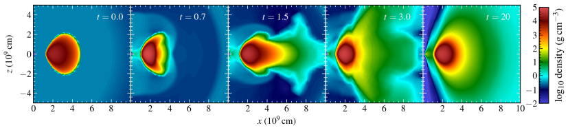
Figure 23: Relaxation of the torus with self-gravity and no other source terms. Shown is the density of the fiducial model at various times in units of the orbital time at the initial density peak (equation 13).

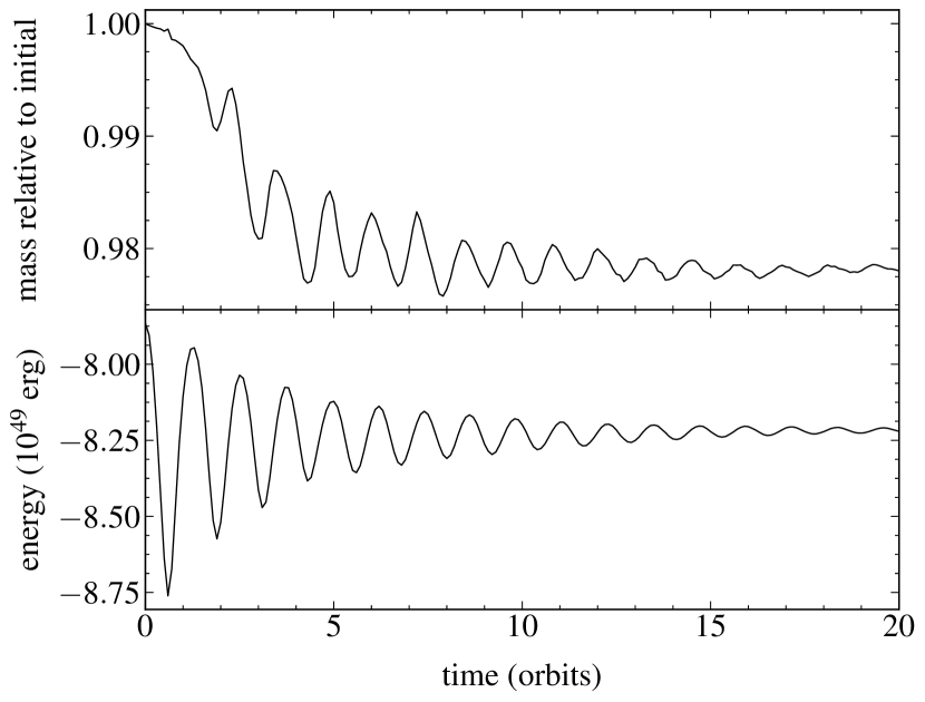
Figure 24: Relaxation of the initial torus with self-gravity, starting from an initial condition calculated with the gravity of the central object only. Shown are the torus mass relative to its initial value, restricted to densities higher than $10^{-3}$ times the maximum (top), and the total torus energy (bottom). Parameters correspond to model CO+NS(l).

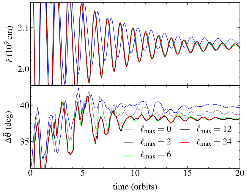
Figure 25: Density weighted radius (top) and opening angle from the equator (bottom) as a function of time, for different values of the maximum Legendre index $\ell_{\rm max}$ in the multipole expansion (equation 30). Torus parameters correspond to our fiducial model, relaxed in self-gravity without other source terms. See the text for the definition $\tilde{r}$ and $\Delta\tilde{\theta}$.

Appendix B Construction of initial torus

B.1 Equilibrium torus without self-gravity

As a starting point for the initial condition, we construct an equilibrium torus with constant entropy $s$, angular momentum, and composition $\mathbf{X}$. By solving the Bernoulli equation (e.g., Papaloizou & Pringle 1984), we obtain an expression for the specific enthalpy of the torus as a function of position, given a central mass $M_{\rm c}$, radius of density maximum in the torus $R_{\rm t}$ (set to the circularization radius of the tidally-disrupted white dwarf; Paper I), and a dimensionless ‘distortion parameter’ $d$ (which is a function of the torus entropy or $H/R$, see e.g., Stone et al. 1999)

$$w(r,\theta)=\frac{GM_{\rm c}}{R_{\rm t}}\left[\frac{R_{\rm t}}{r}-\frac{1}{2}\frac{R_{\rm t}^{2}}{(r\sin\theta)^{2}}-\frac{1}{2d}\right],$$ (45)

where $w=e_{\rm int}+p/\rho$ is the specific enthalpy of the fluid.

For fixed entropy and composition, there is also a one-to-one thermodynamic mapping between the enthalpy and density $w(\rho)|_{s,\mathbf{X}}$ from the equation of state. Inverting this function in combination with equation (45) yields the mass of the torus after spatial integration. The limits of integration are obtained by setting the left-hand side to zero in equation (45). An iteration is required to find the distortion parameter $d$ that yields the desired torus mass $M_{\rm t}$ [which amounts to solving for the function $d(s)$]. Note that the circularization radius (and thus $R_{\rm t}$) is a function of the torus mass and central object mass, hence $M_{\rm t}$ and $R_{\rm t}$ are not independent in this problem.

Figure 22 shows properties of these tori as a function of mass, for three different compositions. Our fiducial C/O WD of mass $M_{\rm wd}=0.6M_{\odot}$ with distortion parameter $d=1.5$ has an entropy $3k_{\rm B}$ per baryon, has very small degree of electron degeneracy, and a small contribution of radiation to the total pressure. Helium WDs of the same mass and distortion parameter have higher entropy, lower contribution of radiation pressure, and higher degeneracy. Increasing the WD mass at constant distortion parameter decreases the entropy, decreases the contribution of radiation pressure, and increases electron dengeneracy. Our fiducial ONe WD has very similar entropy and degeneracy level compared to the fiducial CO WD, but with a higher relative contribution from radiation to the total pressure.

B.2 Relaxation with self-gravity

We obtain a quiescent initial torus with self-gravity by evolving the initial torus solution obtained without self-gravity (§B.1) for $20$ orbits without any other source terms. The torus undergoes radial and vertical oscillations as it adjusts to the new gravitational field, eventually reaching a new equilibrium configuration. Figure 23 shows snapshots in the evolution of the fiducial $0.6M_{\odot}$ CO WD, illustrating the amplitude of these oscillations. The new radius of maximum density is $5\%$ smaller than the original, and the maximum density is a factor $1.6$ higher.

The relaxation process results in the ejection of some mass to large radii. Figure 24 shows that about $2\%$ of the mass contained in material denser than $10^{-3}$ times the maximum density is redistributed to larger radii. The frequency of the oscillations is approximately the orbital frequency at the density maximum. Figure 24 also shows the total energy of the torus, which undergoes oscillations of decreasing amplitude, eventually settling into a new equilibrium value. By the time we stop the relaxation, the amplitude of the oscillations has decrease to about $1\%$.

We also use this torus relaxation process to find the optimal Legendre index at which to truncate the multipole expansion (equation 30). We perform the relaxation process over 20 orbits for our fiducial torus using different values of the maximum Legendre index $\ell_{\rm max}$, with a reference value of $12$ as recommended by Müller & Steinmetz (1995). Convergence is quantified by the radial position of the torus and its opening angle. We define these quantities as an average radius $\tilde{r}$, weighted by the angle-averaged density profile, and the opening polar angle $\Delta\tilde{\theta}$ from the equator (at a constant radius $r=2\times 10^{9}$ cm) at which the density drops to $10^{-3}$ of its maximum value in the simulation. Figure 25 shows the evolution of these two metrics as a function of time for different values of $\ell_{\rm max}$. The evolution is essentially converged after $\ell_{\rm max}=6$, with $\ell_{\rm max}=12$ and $24$ causing an indistinguishable change relative to each other. We therefore adopt $\ell_{\rm max}=12$ for all of our simulations.

Figure 26: Absolute value of the mass accretion rate as a function of radius, averaged in time and within $30$ deg of the equatorial plane, for selected models, as labeled. Top: ONe WD model with non-spinning BH at the center (large boundary: blue, small boundary: red), the dashed line indicates the position of the ISCO radius. Bottom: fiducial WD+NS model (large radius: blue, small radius: red). The dashed line is the same power-law fit ($\propto r^{0.71}$) to the accretion rate as in Figure 16.

Appendix C Long-term accretion rate at the central object

Despite the fact that our fully global (“small boundary”) models cannot be evolved for long enough to obtain a reliable long-term measure of the accretion rate at the central object (to assess jet or fallback power, etc.), we can still estimate this quantity from our large boundary models by examining the radial behavior of the accretion rate, as shown in Figure 26.

A general feature of large boundary models is that the placement of an outflow boundary condition at a radius when the flow is subsonic alters the behavior compared to what it would be had that boundary not be there. Figure 26 shows that there is an increase in the accretion rate by a factor of a few as this boundary is approached, deviating from the power-law behavior at larger radii.

In the case of fully global BH models, the boundary is placed midway between the ISCO and the horizon, where the flow is supersonic and thus causally disconnected from that at larger radii. Figure 26 shows that the ISCO results in an increase in the accretion rate similar to that obtained when placing the boundary further out, such that the value at the ISCO is essentially the same as that measured at the innermost active radius in the large boundary run. We therefore estimate the accretion rate onto the black hole, for Figure 1, as simply the value of the accretion rate at the smallest radius in the large boundary run.

When a NS sits at the center, the discrepancy in the accretion rate at the smallest radii between the large- and small boundary runs is more significant. Nevertheless, we can estimate a reasonable value by measuring the accretion rate in the large boundary model at a radius where the power-law behavior still holds, and then extrapolating using the power-law exponent, as indicated in Figure 26. In Figure 1, the accretion rate for the two NS models is obtained by measuring it at $r=10^{8}$ cm and applying a suppression factor $(10^{-2})^{0.7}$. This assumes that the radial exponent of the accretion rate remains constant in time, which is roughly satisfied.

References

- Arnett (1979) Arnett W. D., 1979, ApJ, 230, L37
- Artemova et al. (1996) Artemova I. V., Bjoernsson G., Novikov I. D., 1996, ApJ, 461, 565
- Bahramian et al. (2017) Bahramian A., et al., 2017, MNRAS, 467, 2199
- Bobrick et al. (2017) Bobrick A., Davies M. B., Church R. P., 2017, MNRAS, 467, 3556
- Chen et al. (2019) Chen P., et al., 2019, ApJL, submitted, arXiv:1905.02205
- Colella & Woodward (1984) Colella P., Woodward P. R., 1984, JCP, 54, 174
- Dan et al. (2014) Dan M., Rosswog S., Brüggen M., Podsiadlowski P., 2014, MNRAS, 438, 14
- Datta & Mukhopadhyay (2019) Datta S. R., Mukhopadhyay B., 2019, MNRAS, 486, 1641
- Dexter & Kasen (2013) Dexter J., Kasen D., 2013, ApJ, 772, 30
- Drout et al. (2014) Drout M. R., et al., 2014, ApJ, 794, 23
- Dubey et al. (2009) Dubey A., Antypas K., Ganapathy M. K., Reid L. B., Riley K., Sheeler D., Siegel A., Weide K., 2009, J. Par. Comp., 35, 512
- Eggleton (1983) Eggleton P. P., 1983, ApJ, 268, 368
- Fernández et al. (2015) Fernández R., Kasen D., Metzger B. D., Quataert E., 2015, MNRAS, 446, 750