LEMO: Learn to Equalize for MIMO-OFDM Systems with Low-Resolution ADCs

Abstract

This paper develops a new deep neural network optimized equalization framework for massive multiple input multiple output orthogonal frequency division multiplexing (MIMO-OFDM) systems that employ low-resolution analog-to-digital converters (ADCs) at the base station (BS). The use of low-resolution ADCs could largely reduce hardware complexity and circuit power consumption, however, it makes the channel station information almost $blind$ to the BS, hence causing difficulty in solving the equalization problem. In this paper, we consider a supervised learning architecture, where the goal is to learn a representative function that can predict the targets (constellation points) from the inputs (outputs of the low-resolution ADCs) based on the labeled training data (pilot signals). Especially, our main contributions are two-fold: 1) First, we design a new activation function, whose outputs are close to the constellation points when the parameters are finally optimized, to help us fully exploit the stochastic gradient descent method for the discrete optimization problem. 2) Second, an unsupervised loss is designed and then added to the optimization objective, aiming to enhance the representation ability (so-called generalization). Lastly, various experimental results confirm the superiority of the proposed equalizer over some existing ones, particularly when the statistics of the channel state information are unclear.

I Introduction

Massive MIMO is foreseen to be one of the key enablers for the future generation communication system, in which the spectral efficiency is expected to be several-order higher than that in the current one [1]. Scaling up the number of the antennas in the BS can offer numerous advantages [2] while exhibiting the gigantic energy consumptions. To alleviate this predicament, equipping the BS with low-resolution ADCs/DACs can greatly reduce energy consumptions [3, 4, 5, 6] in the massive MIMO system.

Last few years have witnessed the publication of many technical results reporting the performance of the massive MIMO system with low-resolution ADCs. In this work, we will focus on the data equalization problem. For the frequency-flat channel, the authors of [7] show that the performance gap between the quantized MIMO system and ideal one can be approached by increasing the number of antennas. Similar results have been reported in the frequency-selective case, i.e., single-cell sparse broadband massive MIMO [8] and then multi-cell millimeter wave massive MIMO [9].

Most of these works are based on the Bussgang theorem [10], with which the severe nonlinearity introduced by the ADCs is approximately expressed by a linear combination of the input and a distortion term. The Bussgang theorem based data equalization methods have low computational complexity comparable to the classical linear data equalization methods. On the other hand, they have to suffer from the performance saturation pain in the mid-to-high SNR regime [11, 12, 13]and attest to a low degree of adaptability in practical 5G millimeter-wave massive MIMO systems [14].

It is hard to understand the nonlinearity introduced by the ADCs with a tractable mathematical model. As a result, the best approach for data equalization problem is unclear. Alternatively, it would be interesting to comprehend (or learn) the nonlinear structure of the employed ADCs leveraging the potential of the deep learning based methods [15].

Recently, the deep learning based detection methods have been proposed for MIMO-OFDM systems with ideal DACs [16, 17]. It has been shown that deep learning based method has comparable performance with the minimum mean-square error receiver and shows robustness in the case of nonlinear clipping noise. The authors of [18] use a recurrent neural network based approach to detect data sequences in molecular communication systems with blind channel state information. Besides, supervised-learning-aided estimator has been proposed for the frequency-flat MIMO system with low-resolution ADCs [19].

In this paper, instead of relying solely on deep learning methods, we propose a new deep neural network optimized equalization framework, jointly exploiting structural knowledge from MIMO systems and harnessing the power of unsupervised deep learning, for MIMO-OFDM systems with low-resolution ADCs.

The remainder of this paper is structured as follows. Section II introduces the signal model for the MIMO-OFDM systems with low-resolution ADCs, in which the Bussgang theorem based linearized data equalization method is discussed. In Section III, we detail the design of the proposed method. A coarse deep neural network based equalizer, following the structure of the widely-used supervised learning method, is firstly proposed. To enhance the generalization of proposed equalizer, a fine deep neural network based equalizer is then developed by leveraging the knowledge from the unsupervised learning. Furthermore, numerical case studies in Section IV are provided to evaluate the performance of the proposed approach. Lastly, the conclusion and acknowledgment of this paper are given in Section V and Section VI, respectively.

$Notations:$ Throughout this paper, vectors and matrices are given in lowercase and uppercase boldface letters, e.g., $\bf{x}$ and $\bf{X}$, respectively. We use ${{\bf{X}}^{H}}$ to denote the conjugate transpose of ${\bf{X}}$. The $k$th row and $l$th column element of ${\bf{X}}$ is denoted by ${\left[{\bf{X}}\right]_{kl}}$. We use $\Re\left({\bf{x}}\right)$, $\Im\left({\bf{x}}\right)$, and ${\left\|{\bf{x}}\right\|_{2}}$ to represent the real part, the imaginary part, $\ell_{2}$-norm of vector ${\bf{x}}$.

II PRELIMINARIES

II-A MIMO-OFDM System Model

We consider a MIMO-OFDM uplink system [20] with $R$ receive antennas at the BS, serving simultaneously $K$ single-antenna user terminals (UTs) over $N$ subcarriers. We use ${\bf{h}}_{rk}\in{\mathbb{C}^{\mu}}$ to denote the channel impulse response of $\mu$ taps between the $r$-th receive antenna and the $k$-th transmit antenna, for $k=1,\cdots,K$, $r=1,\cdots,R$. Let ${\bf{X}}_{k}\in{\mathbb{C}^{N\times T}}$ be a sequence of $T$ OFDM symbols to be sent from the $k$-th antenna. After removing the cyclic prefix and applying an IFFT, the received signal ${{\bf{Y}}_{r}}\in{\mathbb{C}^{N\times T}}$ at the $r$-th receive antenna reads

$${{\bf{Y}}_{r}}=\sum\limits_{k=1}^{K}{{{\bf{H}}_{rk}}{{\bf{F}}^{H}}{{\bf{X}}_{k}}+{{\bf{V}}_{r}}},$$ (1)

where ${{\bf{H}}_{rk}}$ denotes the circulant channel convolution matrix, ${\bf F}$ is the $unitary$ discrete Fourier transform (DFT) matrix [20] of dimension $N\times N$ and the elements of ${{\bf{V}}_{r}}$ are assumed to be identically independent distributed zero-mean Gaussian variables with variance $\sigma^{2}$.

II-B Quantization

For the MIMO-OFDM uplink system with low-resolution ADCs, it is assumed that the real and imaginary parts of received signals are quantized separately by a $B$-bit symmetric uniform quantizer $Q$, denoted by

$${\bf{z}}=Q({\bf{y}})={Q(\Re\left({{\bf{y}}}\right))}+{jQ(\Im\left({{\bf{y}}}\right))}.$$ (2)

Specially, the real-valued quantizer $Q(.)$ maps the input to a set of labels $\Omega=\left\{{{l_{0}},{\kern 1.0pt}\cdots,{l_{{2^{B}-1}}}}\right\}$, which are determined by the set of thresholds $\Gamma=\left\{{{\tau_{0}},{\kern 1.0pt}\cdots,{\tau_{{2^{B}}}}}\right\}$, such that $-\infty={\tau_{0}}<\cdots<{\tau_{{2^{B}}}}=\infty$. For a $B$-bit ADC with step size $\Delta$, the thresholds and quantization labels are respectively given by [7, 21]

$${l_{b}}=\Delta\left({b-\frac{{{2^{B}-1}}}{2}}\right),\ b=0,\cdots,{2^{B}-1},$$ (3)

and

$${\tau_{b}}=\Delta\left({i-{2^{B-1}}}\right),\ b=1,\cdots,{2^{B}}-1.$$ (4)

In the case of 1 bit ADCs, the output set reduces to ${\Omega_{1}}=\left\{{\pm\frac{\Delta}{2}\pm{\rm i}\frac{\Delta}{2}}\right\}$.

From (1) and (2), the resulting quantized signals yield

$${{\bf{Z}}_{r}}=Q\left({{{\bf{Y}}_{r}}}\right)=Q\left({\sum\limits_{k=1}^{K}{{{\bf{H}}_{rk}}{{\bf{F}}^{H}}{{\bf{X}}_{k}}+{{\bf{V}}_{r}}}}\right).$$ (5)

II-C Data Equalization and Linearized Solution

The serve nonlinearity of (2) makes the channel station information almost $blind$ to the BS, resulting in a challenging work for data equalization in quantized frequency-selective MIMO systems. Recently, as shown in the Section I, many researchers proposed to represent the nonlinearity of a Gaussian signal by the sum of a linear transformation and an uncorrelated quantization error term, according to the Bussgang theorem [10]. Following the Bussgang theorem, (5) can be approximately represented by

$${{\bf{Z}}_{r}} =Q\left({\sum\limits_{k=1}^{K}{{{\bf{H}}_{rk}}{{\bf{F}}^{H}}{{\bf{X}}_{k}}+{{\bf{V}}_{r}}}}\right)$$

$$={\bf{G}}\left({\sum\limits_{k=1}^{K}{{{\bf{H}}_{rk}}{{\bf{F}}^{H}}{{\bf{X}}_{k}}+{{\bf{V}}_{r}}}}\right)+{\bf{W}}_{r}$$

$$={\bf{G}}\sum\limits_{k=1}^{K}{{{\bf{H}}_{rk}}{{\bf{F}}^{H}}{{\bf{X}}_{k}}}+{\bf{D}}_{r},$$ (6)

where ${\bf{G}}$ is a diagonal matrix and ${\bf{D}}_{r}$ is referred to the quantization error. The circulant channel matrix has an eigenvalue decomposition

$${{\bf{H}}_{{r}{k}}}={{\bf{F}}^{{H}}}{{\bf{\Lambda}}_{{r}{k}}}{\bf{F}},$$ (7)

where ${{\bf{\Lambda}}_{{r}{k}}}$ is a diagonal matrix and ${{\bf{\Lambda}}_{{r}{k}}}={\mathop{\rm diag}\nolimits}\left\{{\sqrt{N}{\bf{F}}_{N\times\mu}^{{H}}{{\bf{h}}_{{r}{k}}}}\right\}$. Substituting (7) into (II-C) can give the subcarrier-wise input-output relationship:

$${{\bf{Z}}_{n}}=\rho{{\bf{H}}_{n}}{{\bf{X}}_{n}}+{{{\bf{\tilde{D}}}}_{n}},$$ (8)

where $\rho$ is the Bussgang decomposition factor. Then the Bussgang theorem based data equalization problem can be formulated as

$$\begin{array}[]{*{20}{c}}{\min}&{\sum\limits_{n=1}^{N}{\left\|{{{\bf{Z}}_{n}}-\alpha{{\bf{H}}_{n}}{{\bf{X}}_{n}}}\right\|_{2}^{2}}}\\ {{\mathop{\rm s.t.}}}\nolimits&{{{\left[{{{\bf{X}}_{u}}}\right]}_{ij}}\in\Omega}\end{array},$$ (9)

where $\Omega$ is the set of the constellation points. Discarding the nonconvex constraint ${{{\left[{{{\bf{X}}_{u}}}\right]}_{ij}}\in\Omega}$, one can use the minimum mean squared error (MMSE) based method [22] for the channel estimation and then data equalization. Unluckily, such a linearized data equalization method has to suffer from the performance saturation in the mid-to-high SNR regime. Specially, the BER curves achievable with linearized data equalization methods saturate at certain finite SNR, above which no further improvement can be obtained. As a result, it is vital to understanding the nonlinearity of (2) by the new techniques, i.e., the deep neural networks based methods.

III LEMO: Learn to Equalize for MIMO-OFDM

Figure 1: The MIMO-OFDM system with low-resolution ADCs and the proposed deep neural network based equalizer.

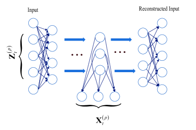
For the coarsely quantized MIMO-OFDM system, the true channel state information is almost completely unknown, the best method to data equalization becomes unclear. As shown in Fig. 1, we propose a deep learning based method to train a data-driven detector to determine transmitted symbols from pilots.

III-A Coarse Deep Neural Network based Equalizer

We start by applying the supervised deep learning [15] for data equalization in quantized MIMO-OFDM system. The employed method in subsection is referred to the coarse deep neural network (CDNN) based equalizer.

III-A1 Data Preprocessing

Generally, the supervised deep learning based approach has two parts: Offline training and online test. Let $T$ be the number of collected data samples. For $t=1,\cdots,T$, we use

$$\left\{{{{\bf{Z}}_{t}},{{\bf{X}}_{t}}}\right\}=\left[{\begin{array}[]{*{20}{c}}{\underbrace{\left\{{{\bf{Z}}_{t}^{\left(p\right)},{\bf{X}}_{t}^{\left(p\right)}}\right\}}_{{\rm{pilot\ singal}}}}&{\underbrace{\left\{{{\bf{Z}}_{t}^{\left(t\right)},{\bf{X}}_{t}^{\left(t\right)}}\right\}}_{{\rm{test\ signal}}}}\end{array}}\right]$$

to represent data collected at $t$-th sampling. In this paper, the elements of ${{\bf{Z}}_{t}}$ and ${{\bf{X}}_{t}}$ are the subcarrier-wise real-valued received signals (outputs of low-resolution DACs) and the transmitted signals, respectively.

III-A2 Network Parameters Optimization

At the offline training stage, the pilot data set:

$$\left\{{{{\bf{Z}}^{\left(p\right)}},{{\bf{X}}^{\left(p\right)}}}\right\}=\left\{{\left({{\bf{Z}}_{1}^{\left(p\right)},{\bf{X}}_{1}^{\left(p\right)}}\right),\cdots,\left({{\bf{Z}}_{T}^{\left(p\right)},{\bf{X}}_{T}^{\left(p\right)}}\right)}\right\}$$

is used to find the optimal set of parameters of a $U$-layer neural network by solving the optimization problem:

$${\cal L}\left(\Theta_{0}\right)=\mathop{{\rm{argmin}}}\limits_{\Theta_{0}}\left\|{{{\bf{Z}}^{\left(p\right)}}-{\varphi_{S}}\left({{{\bf{W}}_{S}}{{{\bf{\tilde{X}}}}^{\left(p\right)}}}\right)}\right\|_{2}^{2},$$ (10)

where

$${{{\bf{\tilde{X}}}}^{\left(p\right)}}={\varphi_{U}}\left({{{\bf{W}}_{U}}\cdots{\varphi_{1}}\left({{{\bf{W}}_{1}}{{\bf{X}}^{\left(p\right)}}}\right)}\right),$$

for $u=1,\cdots,U$, $\varphi_{u}$ is the activation function and ${\bf{W}}_{u}$ are weight matrix at $u$-th layer. $\varphi_{S}$ is a specially designed activation which will be explained latter. The parameters ${\Theta_{0}=\left\{{{{\bf{W}}_{1}},\cdots,{{\bf{W}}_{U}},{{\bf{W}}_{S}}}\right\}}$ are updated to minimize the expected loss (10) by using a stochastic descent based method [15], i.e., stochastic gradient decent (SGD), or Adam.

The deep learning based equalizer described above tries to generate a nonlinear relationship between the transmitted signals and the quantized received signals according to the supervised task, hopefully aiming at understanding (or learning) the true channel matrix information that has been almost $destroyed$ by the use of low-resolution ADCs.

However, solely training a supervised neural network is likely to handle a problem with under-constrained configurations, and will find a solution that can well fit the training data but can not generalize well [23], especially in the case of neural discrete representation learning (the data equalization problem is itself a discrete optimization problem [22]). These limitations motivate us to design a fine deep neural network (FDNN) based equalizer .

III-B Fine Deep Neural Network based Equalizer

Developing a deep neural network with high generalization ability plays a key role for the data equalization of the quantized frequency-selective MIMO systems. Generally, increasing the number of the layers and the number of neurons in a layer can help improve the generalization ability of deep neural networks [15]. However, training a very deep neural network has to face up with the vanishing or exploding gradient problem [24]. Besides, the real time requirement prevents the widespread use of the very deep neural network.

III-B1 The Skew-symmetric Weights Matrix

We stat with a simple example. Let ${\bf x}$ and ${\bf y}$ be two complex-valued vectors and ${\bf H}$ a complex-valued matrix. The equation

$${\bf{y=Hx}}$$

equals to

$$\left[{\begin{array}[]{*{20}{c}}{{\mathop{\rm Re}\nolimits}\left\{{\bf{y}}\right\}}\\ {{\mathop{\rm Im}\nolimits}\left\{{\bf{y}}\right\}}\end{array}}\right]=\left[{\begin{array}[]{*{20}{c}}{{\mathop{\rm Re}\nolimits}\left\{{\bf{H}}\right\}}&{-{\mathop{\rm Im}\nolimits}\left\{{\bf{H}}\right\}}\\ {{\mathop{\rm Im}\nolimits}\left\{{\bf{H}}\right\}}&{{\mathop{\rm Re}\nolimits}\left\{{\bf{H}}\right\}}\end{array}}\right]\left[{\begin{array}[]{*{20}{c}}{{\mathop{\rm Re}\nolimits}\left\{{\bf{x}}\right\}}\\ {{\mathop{\rm Im}\nolimits}\left\{{\bf{x}}\right\}}\end{array}}\right].$$

In this work, we focus on the real-valued deep neural network, whose weights structure should be accommodated to complex-valued data. Let

$${{\bf{W}}_{i}}=\left[{\begin{array}[]{*{20}{c}}{{\bf{W}}_{i}^{\left(1\right)}}&{{\bf{W}}_{i}^{\left(2\right)}}\\ {{\bf{W}}_{i}^{\left(3\right)}}&{{\bf{W}}_{i}^{\left(4\right)}}\end{array}}\right]$$

be the weight matrix in $i$-th layer. In the training stage, we set ${{\bf{W}}_{i}^{\left(4\right)}}={{\bf{W}}_{i}^{\left(1\right)}}$ and ${{\bf{W}}_{i}^{\left(3\right)}}=-{{\bf{W}}_{i}^{\left(2\right)}}$, which means only half of the weight matrix will be updated. This simple operation not only makes the proposed network suitable for complex-valued OFDM symbols training but also helps to reduce computational complexity.

III-B2 Activation Function Design

Figure 2: Plot of the proposed functions $f\left({\alpha,\beta,x}\right)$ for $\alpha=1/\sqrt{2}$, $\beta=1,10,100$.

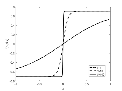
As shown in (9), the data equalization problem itself is a non-convex optimization problem. Discarding the nonconvex constraint yields the suboptimal solution. In this work, we design a new activation function to help us fully exploit the stochastic gradient descent method for the discrete optimization problem. Specially, in the case of QPSK signaling and as shown in Fig. 2, we propose to use the activation function:

$$f\left({\alpha,\beta,x}\right)=\alpha\frac{{{e^{\beta x}}-{e^{-\beta x}}}}{{{e^{\beta x}}+{e^{-\beta x}}}},$$ (11)

where $\alpha$ is the magnitude of the transmitted signal. $\beta$ is a trainable parameter that controls the layer’s outputs, which will be sufficiently close to the constellation points. Since the data in the higher-order modulation can be represented by a linear combination of the QPSK data [25], we leave out the design for the higher-order modulation.

III-B3 Generalization Enhancement

In this paper, motivated by the pioneer work [26], we propose to improve the representation of the employed neural network by adding an unsupervised loss to (10). Specially, the proposed neural network based equalizer tries to update the neural network parameters ${\Theta_{1}=\left\{{{{\bf{W}}_{U+1}},\cdots,{{\bf{W}}_{2U}}}\right\}}$ by minimizing

$$\begin{array}[]{*{20}{c}}{\mathop{{\rm{argmin}}}\limits_{\Theta}}&{{\cal L}\left(\Theta_{0}\right)+\lambda{{\cal L}_{1}}\left({{\Theta_{1}}}\right)}\end{array},$$ (12)

where

$${{\cal L}_{1}}\left({{\Theta_{1}}}\right)=\left\|{{{\bf{X}}^{\left(p\right)}}-{\varphi_{2U}}\left({{{\bf{W}}_{2U}}\cdots{\varphi_{U+1}}\left({{{\bf{W}}_{1}}{{{\bf{\tilde{X}}}}^{\left(p\right)}}}\right)}\right)}\right\|_{2}^{2},$$

$\Theta={{\Theta_{0}}\cup\Theta_{1}}$, and $\lambda$ is the penalty parameter that balances $\mathcal{L}\left(\Theta_{0}\right)$ and $\mathcal{L}_{1}\left(\Theta_{1}\right)$. We use an unsupervised loss to promote the generalization of the proposed FDNN equalizer for three reasons:

• The unsupervised loss in (12) itself is a denoising autoender [27] that may help to eliminate the noise from the data samples.

• It has been shown in previous studies that learning multi-task jointly can improve the generalization error bounds [28]. In our case, we jointly minimize $\mathcal{L}\left(\Theta\right)$ and $\mathcal{L}_{0}\left(\Theta_{0}\right)$.

• A nonlinear autoender (12) have been indeed found to be helpful for key feature extraction [27, 15]. In our case, it helps to represent ${{\bf{X}}^{\left(p\right)}}$ of high-dimension from ${{\bf{U}}^{\left(p\right)}}$ of low-dimension (the number of users is much less than the number of received antennas).

III-C Algorithm Implementation and Discussions

The network model we use consists of eight layers. The numbers of neurons in each layer are $2R$, $12U$,$6U$, $2U$, $2R$, $2R$, $2R$, and $2U$, respectively. The batch size e Every 1$k$ bits of the data are grouped and then inputed into the network for training. The Relu function is used as the activation function except the layer $S$.

The test complexity of the proposed method involves simple matrix-vector multiplications and has complexity of order $O\left({40{R^{2}}U}\right)$. In a MIMO system with 128 transmit antennas and 8 UEs, the average runtime for the proposed method and MMSE are 0.0715 ms and 0.00922 ms, respectively. The runtime performance demonstrates the feasibility of the practical implementation of the proposed method.

IV Case Studies

In this section, using the Tensorflow platform [29], we evaluate the performance of the proposed equalizers via numerical simulations on a PC with an Intel Core i7-7700K CPU and two NVIDIA GTX 1080 Ti GPUs.

IV-A System and Network Parameters Setup

We consider a QPSK modulated MIMO-OFDM system with 128 BS antennas, simultaneously serving 8 users. Following the IEEE 802.11a standard, we use 64 subcarriers in an OFDM block. The channel tap length is $\mu=8$. It is assumed that the coherence time is $T=64$. A typical urban environment with max delay 16 is considered.

TABLE I: The network parameters employed in the proposed equalizer.

	Network Parameters
	Layer	Activation	Weights
$L_{1}$	Input	-	-
$L_{2}$	Full-Connected	relu	$256\times 96$ GM
$L_{3}$	Full-Connected	relu	$96\times 48$ GM
$L_{4}$	Full-Connected	relu	$48\times 16$ GM
$L_{5}$	Full-Connected	relu	$16\times 48$ GM
$L_{6}$	Full-Connected	relu	$48\times 96$ GM
$L_{7}$	Full-Connected	relu	$96\times 256$ GM
$S$ a	Full-Connected	$f\left({\alpha,\beta,x}\right)$	$16\times 16$ IM
aThis layer is connected to layer $L_{4}$ as shown in Fig. 1.

Tab. I illustrates the parameters in the proposed network i.e., the layer size, layer initializations, and activation functions. The notation GM in Tab. I means the Gaussian matrix whose elements have zero mean and variance 0.01. IM means the identity matrix. The parameter $\beta$ in the proposed activation function $f\left({\alpha,\beta,x}\right)$ will be updated from 1 to 100 to find the optimal $\beta$ on every mini-batch training.

IV-B Effect of the Quantization Level

Figure 3: BER curves of the proposed equalizer with different quantization levels.

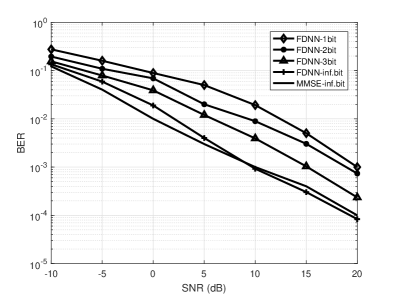
In Fig. 3, we investigate the BER performance of the proposed equalizer with different quantization levels. The benchmark equalizer considered is the MMSE equalizer with infinite-resolution ADCs (MMSE-inf.bit). It can be observed that the performance of proposed FDNN equalizer improve as a result of a increased bits of ADCs. The performance gap between the MMSE-inf.bit equalizer and the proposed equalizer is negligible when the number of the bits of ADCs is no less than 2. Interestingly, the proposed FDNN equalizer with infinite-resolution ADCs (FDNN-inf.bit) slightly outperforms the MMSE-inf.bit equalizer when the SNR is over 10 dB. These results above demonstrate that the proposed network can nicely approximate the nonlinearity introduced by the employed ADCs.

IV-C The Effect on the Distribution of the Channel Taps

Figure 4: BER curves of the compared equalizers with two kinds of channel taps. The performance is evaluated in a MIMO system with 2-bit ADCs. The number of taps is 24.

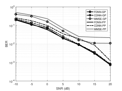
In Fig. 4, we study the performance of the proposed equalizers (CDNN and FDNN) under two kinds of pilots: Gaussian distributed pilots (GP) and Poisson distributed pilots (PP) . Fig. 4 shows BER curves of the MMSE equalizer do not decease distinctly as the SNR increases when the SNR is above 10 dB. On the other hand, the CDNN and FDNN equalizers have robust performance in a wide range of SNR. Besides, it is seen that the proposed FDNN equalizer outperforms the CDNN and MMSE equalizer under scenarios where GD pilots and PD pilots are used. The FDNN equalizer is more robust than the CDNN equalizer in the case of PD pilots. Such an phenomena may be explained by the enhanced generalization of the FDNN.

IV-D The Effect of Pilots Numbers

Figure 5: BER curves of the compared equalizers with different lengths of Gaussian pilots. The performance is evaluated in a MIMO system with 2-bit ADCs.

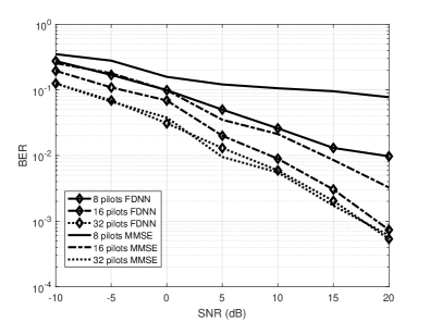
The feedbacks (in this paper, we only consider the number of the pilots) are limited in a real communication system, which reveals another challenge in the design of an effective neural network. In Fig. 5, we show the results of the effect of the pilot numbers.

From Fig. 5, the larger numbers of pilots lead to better performance of all compared equalizers and they have comparable performance when 32 pilots are used. In the case that when only 8 pilots are used, the proposed FDNN equalizer significantly outperforms the MMSE equalizer. The proposed FDNN equalizer and the MMSE equalizer can respectively achieve a target BER of $10^{-3}$ with 8 pilots and 16 pilots, demonstrating the potential for pilots saving.

V Conclusions and Future Work

In this paper, the deep neural network based equalizer has been proposed for the MIMO-OFDM systems with low-resolution ADCs. The experimental results show that the proposed equalizer is robust to different channel taps (i.e., Gaussian, and Poisson) and significantly outperforms the linearized MMSE equalizer. In addition, given a target of bit error rate, the proposed learning architecture with an unsupervised loss is more efficient in terms of the number of pilots, when compared to the learning architecture without such a design or the linearized MSSE equalizer. A key feature of the proposed method is that the employment of all unlabeled data can enhance the quality of the equalization result over different kinds of channel models.

It will be a long way to go regarding the neural networks based approach as a general way for the MIMO equalization. We shall consider the impact of the change of system parameters and integration into full-duplex communication systems. Nonetheless, it is believed that the proposed method has the potential to impact the design of future communication systems. In our future work, we will provide theoretical analysis, i.e., based on the Rademacher complexity analysis [30], for the generalization improvement in the fine deep neural network based equalizer. Besides, it is interesting to investigate how many parameters are needed for training a neural network based method for data equalization problem in MIMO-OFDM systems with low-resolution ADCs.

VI Acknowledgment

The authors would like to thank Dr. Yanwen Fan, from the EECS department of the University of Tennessee, Knoxville, for fruitful discussions in the neural network algorithm implementation.

References

- [1] L. Lu, G. Y. Li, A. L. Swindlehurst, A. Ashikhmin, and R. Zhang, “An overview of massive MIMO: Benefits and challenges,” IEEE J. Sel. Topics Signal Process., vol. 8, no. 5, pp. 742–758, 2014.
- [2] F. Rusek, D. Persson, B. K. Lau, and E. G. Larsson, “Scaling up MIMO: Opportunities and challenges with very large arrays,” IEEE Signal Process. Mag., vol. 30, no. 1, pp. 40–60, 2012.
- [3] S. Wang, Y. Li, and W. Jing, “Multiuser detection in massive spatial modulation MIMO with low-resolution ADCs,” IEEE Trans. Wireless Commun., vol. 14, no. 4, pp. 2156–2168, 2015.
- [4] S. Wang and Z. Lin, “Signal processing in massive MIMO with iq imbalances and low-resolution ADCs,” IEEE Trans. Wireless Commun., vol. PP, no. 99, pp. 1–1, 2016.
- [5] F. Wang, J. Fang, H. Li, and S. Li, “Quantization design and channel estimation for massive MIMO systems with one-bit ADCs,” IEEE Trans. Veh. Technol., vol. PP, no. 99, 2017.
- [6] L. Chu, F. Wen, L. Li, and R. C. Qiu, “Efficient nonlinear precoding for massive MIMO downlink systems with 1-bit DACs,” IEEE Trans. Wireless Commun., vol. 18, no. 9, pp. 4213–4224, 2019.
- [7] S. Jacobsson, G. Durisi, M. Coldrey, U. Gustavsson, and C. Studer, “Throughput analysis of massive MIMO uplink with low-resolution ADCs,” IEEE Trans. Wireless Commun., vol. 16, no. 6, pp. 4038–4051, 2017.
- [8] A. Mezghani and A. L. Swindlehurst, “Blind estimation of sparse broadband massive MIMO channels with ideal and one-bit ADCs,” IEEE Trans. Signal Process., vol. PP, no. 99, pp. 1–1, 2017.
- [9] J. Xu, W. Xu, H. Zhang, G. Y. Li, and X. You, “Performance analysis of multi-cell millimeter wave massive MIMO networks with low-precision ADCs,” IEEE Trans. Commun., pp. 1–1, 2018.
- [10] J. J. Bussgang, “Crosscorrelation functions of amplitude-distorted Gaussian signals,” MIT Res. Lab. Electron., vol. 216, 1952.
- [11] Y.-S. Jeon, N. Lee, S.-N. Hong, and R. W. Heath, “One-bit sphere decoding for uplink massive MIMO systems with one-bit ADCs,” IEEE Trans. Commun., vol. 17, no. 7, pp. 4509–4521, 2018.
- [12] N. J. Myers and R. W. Heath, “Message passing-based joint cfo and channel estimation in millimeter wave systems with one-bit ADCs.” IEEE Trans. Commun., pp. 1–14, 2019.
- [13] C. K. Wen, C. J. Wang, J. Shi, K. K. Wong, and P. Ting, “Bayes-optimal joint channel-and-data estimation for massive MIMO with low-precision ADCs,” IEEE Trans. Signal Process., vol. 64, no. 10, pp. 2541–2556, 2016.
- [14] J. Zhang, L. Dai, L. Xu, L. Ying, and L. Hanzo, “On low-resolution ADCs in practical 5g millimeter-wave massive MIMO systems,” IEEE Communications Magazine, vol. PP, no. 99, pp. 2–8, 2018.
- [15] Y. Lecun, Y. Bengio, and G. Hinton, “Deep learning.” Nature, vol. 521, no. 7553, p. 436, 2015.
- [16] H. Ye, G. Y. Li, and B. H. Juang, “Power of deep learning for channel estimation and signal detection in OFDM systems,” IEEE Wireless Commun. Lett., vol. 7, no. 1, pp. 114–117, 2018.
- [17] H. He, C. Wen, S. Jin, and G. Y. Li, “A model-driven deep learning network for MIMO detection,” in IEEE GlobalSIP, 2018, pp. 584–588.
- [18] N. Farsad and A. Goldsmith, “Neural network detection of data sequences in communication systems,” IEEE Trans. Signal Process., vol. 66, no. 21, pp. 5663–5678, 2018.
- [19] Y. S. Jeon, S. N. Hong, and N. Lee, “Supervised-learning-aided communication framework for MIMO systems with low-resolution ADCs,” IEEE Trans. Veh. Technol., vol. PP, no. 99, pp. 1–1, 2018.
- [20] A. Goldsmith, Wireless Communications. New York, NY, USA: Cambridge University Press, 2005.
- [21] L. Chu, F. Wen, and R. C. Qiu, “Eigen-inference precoding for coarsely quantized massive MU-MIMO system with imperfect CSI,” IEEE Trans. Veh. Technol., vol. 68, no. 9, pp. 8729–8743, 2019.
- [22] H. V. Poor, An Introduction to Signal Detection and Estimation (2Nd Ed.). Berlin, Heidelberg: Springer-Verlag, 1994.
- [23] C. Zhang, S. Bengio, M. Hardt, B. Recht, and O. Vinyals, “Understanding deep learning requires rethinking generalization,” CoRR, vol. abs/1611.03530, 2017. [Online]. Available: http://arxiv.org/abs/1611.03530
- [24] B. Hanin, “Which neural net architectures give rise to exploding and vanishing gradients?” in NeurIPS, S. Bengio, H. Wallach, H. Larochelle, K. Grauman, N. Cesa-Bianchi, and R. Garnett, Eds., 2018, pp. 582–591.
- [25] Z. Mao, X. Wang, and X. Wang, “Semidefinite programming relaxation approach for multiuser detection of qam signals,” IEEE Trans. Wireless Commun., vol. 6, no. 12, pp. 4275–4279, 2007.
- [26] D. Erhan, Y. Bengio, A. C. Courville, P. A. Manzagol, and S. Bengio, “Why does unsupervised pre-training help deep learning?” J. Mach. Learn. Res., vol. 11, no. 3, pp. 625–660, 2010.
- [27] P. Vincent, H. Larochelle, I. Lajoie, Y. Bengio, and P. A. Manzagol, “Stacked denoising autoencoders: Learning useful representations in a deep network with a local denoising criterion,” J. Mach. Learn. Res., vol. 11, no. 12, pp. 3371–3408, 2010.
- [28] A. Maurer and M. Pontil, “Excess risk bounds for multitask learning with trace norm regularization,” J. Mach. Learn. Res., vol. 30, pp. 55–76, 2013.
- [29] M. Abadi, P. Barham, J. Chen, Z. Chen, A. Davis, J. Dean, M. Devin, S. Ghemawat, G. Irving, and M. Isard, “Tensorflow: a system for large-scale machine learning,” in 12th USENIX Symposium on Operating Systems Design and Implementation, 2016, pp. 265–283.
- [30] P. Bartlett and S. Mendelson, “Rademacher and gaussian complexities: Risk bounds and structural results,” J. Mach. Learn. Res., vol. Nov., no. 3, pp. 224–240, 2002.