Extrapolation of nuclear structure observables with artificial neural networks

Abstract

Calculations of nuclei are often carried out in finite model spaces. Thus, finite-size corrections enter, and it is necessary to extrapolate the computed observables to infinite model spaces. In this work, we employ extrapolation methods based on artificial neural networks for observables such as the ground-state energy and the point-proton radius. We extrapolate results from no-core shell model (NCSM) and coupled-cluster (CC) calculations to very large model spaces and estimate uncertainties. Training the network on different data typically yields extrapolation results that cluster around distinct values. We show that a preprocessing of input data, and the inclusion of correlations among the input data, reduces the problem of multiple solutions and yields more stable extrapolated results and consistent uncertainty estimates. We perform extrapolations for ground-state energies and radii in ⁴He, ⁶Li, and ¹⁶O, and compare the predictions from neural networks with results from infrared extrapolations.

I Introduction

In nuclear physics, ab initio methods aim to solve the nuclear many-body problem starting from Hamiltonians with two- and three-nucleon forces using controlled approximations Dickhoff and Barbieri (2004); Navrátil et al. (2009); Lee (2009); Barrett et al. (2013); Roth et al. (2012); Dytrych et al. (2013); Hagen et al. (2014); Carlson et al. (2015); Hergert et al. (2016). Most of these methods employ finite model spaces, and this makes it necessary to account for finite-size corrections or to extrapolate the results to infinite model spaces. While light nuclei with large separation energies require little or no extrapolations, finite-size effects are non-negligible in weakly bound nuclei or heavy nuclei. Various empirical extrapolation schemes Horoi et al. (1999); Zhan et al. (2004); Hagen et al. (2007); Forssén et al. (2008); Bogner et al. (2008) have been used. More recently, rigorous extrapolation formulas were derived based on an understanding of the infrared and ultraviolet cutoffs of the harmonic oscillator basis Furnstahl et al. (2012); Coon et al. (2012); More et al. (2013); Furnstahl et al. (2014); König et al. (2014); Wendt et al. (2015); Odell et al. (2016); Forssén et al. (2018). These extrapolation formulas are akin to Lüschers formula Lüscher (1986) derived for the lattice and its extension König and Lee (2018) to many-body systems. Unlike the lattice, however, the harmonic oscillator basis mixes ultraviolet and infrared cutoffs, and this complicates extrapolations. Very recently, Negoita and coworkers Alina Negoita et al. (2018); Negoita et al. (2019) employed artificial neural networks for extrapolations. They trained a network on NCSM results obtained in various model spaces, i.e. for various oscillator spacings $\hbar\omega$ and different numbers $N_{\rm max}\hbar\omega$ of maximum excitation energies. In practical calculations, $N_{\rm max}\approx 10\ldots 20$ in light nuclei. The neural network then predicted extrapolations in very large model spaces of size $N_{\rm max}\sim 100$. Impressively, the neural network also predicted that the ground-state energies and radii cease to depend on the oscillator spacing as $N_{\rm max}$ increases. Negoita and coworkers employed about 100 neural networks, each differed by the initial set of parameters (weights) from which the training started. The resulting distributions for observables occasionally exhibited a multi-mode structure stemming from multiple distinct solutions the neural networks arrived at. In this work, we want to address this challenge and focus on the network robustness and avoidance of multiple solutions.

In recent years, artificial neural networks have been used for various extrapolations in nuclear physics Clark et al. (2001); Athanassopoulos et al. (2004); Costiris et al. (2009); Akkoyun et al. (2013); Utama et al. (2016a, b); Utama and Piekarewicz (2017, 2018); Neufcourt et al. (2018), and for the solution of the quantum many-body system Carleo and Troyer (2017). Artificial neural networks use sets of nonlinear functions to describe the complex relationships between input and output variables. The universality of using artificial neural networks to solve extrapolation problems is largely guaranteed, because no particular analytical functions are needed. Artificial neural networks are controlled by two hyperparameters, i.e. the number of layers and the number of neurons for each layer.

There are still two major challenges when introducing neural networks in extrapolations of results from ab initio computations. Firstly, unlike other applications in which large amounts of training data can be acquired, the inputs provided by the ab initio calculations are limited to small data sets. The statistics is clearly not enough to support the network training without overfitting. Secondly, randomness, caused by the nature of basic network algorithms, is an intrinsic quality of the neural network that conflicts with the high-precision requirement for extrapolations.

In this work, we use an artificial neural network and extrapolate observables computed with the NCSM and CC methods. Besides standard techniques such as regularization, we use interpolation of data to mitigate the overfitting problem and also take into account the correlations in the resulting data set. The random initialization of the network parameters provides us with a “forest” of artificial neural networks. This allows us to gain insights into uncertainties of the extrapolated observables, under the precondition that the distribution of extrapolation results has a single peak.

We note here that the extrapolation problem we are concerned with is special in the sense that a well defined asymptotic value exists for the observable of interest (i.e. an energy or a radius), that there is a simple pattern in the learning data, and that the learning data is already close to this asymptotic value. We will see below that this makes an artificial neural network a useful tool for this kind of extrapolation. Needless to say, for a general problem there is no tool to extrapolate: we cannot extrapolate from available data to next week’s stock market value or next month’s weather. We refer the reader to the literature for attempts to use deep learning in extrapolations Martius and Lampert (2016), and for a counter example Haley and Soloway (1992).

This paper is organized as follows. In the next Section we introduce the theoretical framework and artificial neural networks and present a detailed account of how we construct, train, and use neural networks. We then present and discuss the extrapolation results for ⁴He, ⁶Li, and ¹⁶O. Finally, we summarize our work.

II Theoretical Framework

II.1 Artificial Neural Network Architecture

An artificial neural network is a computing system that consists of a number of interconnected blocks which process the input information and yield an output signal. Modeled loosely after the human brain, the neural network is typically organized by similar blocks called “layers,” and each layer contains a certain number of parallel “neurons.” The numbers of layers and neurons define the depth and the width of the neural network, respectively.

Figure 1: (Color online) Schematic structure of a typical feed-forward neural network.

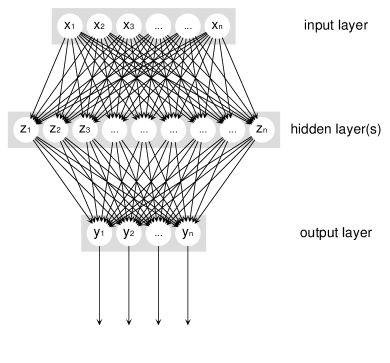
Figure 1 shows the schematic structure of a simple feed-forward neural network. The algorithm basically consists of two parts. First, the input signal $x$ is propagated to the output layer $y$ by a series of transformations. The whole network can be seen as a complex function between the input and output variables. In the simple case with one hidden layer, the function can be written as follow,

$$z_{j}=\displaystyle\sum_{i}x_{i}w_{ij}+b_{j},$$ (1)

with $\sigma$ as the activation function,

$$x^{\prime}_{j}=\sigma(z_{j})$$ (2)

$$y_{k}=\displaystyle\sum_{j}x^{\prime}_{j}w^{\prime}_{jk}+b^{\prime}_{k}.$$ (3)

Here, $x_{i}$ are the input variables, and $y_{k}$ are the output variables. The weights $w~{}(w^{\prime})$ and bias $b~{}(b^{\prime})$ are free parameters of the neural network. There exist a few choices one can make for the activation function $\sigma$, such as the sigmoid, tanh and Rectified Linear units (ReLu). These are non-linear functions which enable the neural network to capture complex non-linear relationships between variables. For the extrapolation we follow Ref. Negoita et al. (2019) and use a smooth activation function that only acts on the hidden layer. Back-propagation is the second part of the algorithm Rumelhart et al. (1986). This is the central mechanism that allows neural network methods to “learn.” The error signals, often referred to as the “loss,” which measure the deviation between the predicted output $y_{\rm{pre}}$ and the training target $y_{\rm{true}}$, are propagated backwards to all the parameters of the network and allow the optimizer to update the network status accordingly. Note that, in practice, the neural network always processes the data in batches, which makes the input (output) signals $x~{}(y)$ matrices and the network functions become matrix operations.

In order to construct the artificial neural network aiming to solve the extrapolation problem, we first need to determine its topological structure. There are a lot of variants for neural networks, such as Recurrent Neural Network (RNN), Long Short-Term Memory (LSTM) and Convolutional Neural Network (CNN), which are designed for various assignments. One should choose the appropriate type of network according to the organizational structure of the dataset and the goal that one wants to achieve. In the case of extrapolation, the data for training is assigned to a structure consisting of three members, namely $\hbar\omega$, $N_{\rm{max}}$, and the corresponding target observables, i.e. the ground-state energy and the point-proton radius. On the other hand, the main purpose of the neural network is to provide reasonable predictions for the observables at any values of $\hbar\omega$ and $N_{\rm{max}}$. In this paper we use the feed-forward neural network, which takes the $\hbar\omega$ and $N_{\rm{max}}$ as two inputs $(x)$ and the target observables as output $(y_{\rm{true}})$. One could as well apply the RNN structure to achieve the same goal. The only difference between the two choices is that the data structure need to be reorganized in terms of sequential observable values with increasing $N_{\rm{max}}$ under the same $\hbar\omega$.

Once the basic structure is decided, the next task is to control the complexity of the network. The network’s ability of describing complex features is determined by the numbers of the hidden layers and neurons in each layer. In other words, the depth and the width of the neural network control the upper limit of the neural network description. Ideally, in order to lower the loss of the training dataset, adding more layers and neurons is always helpful to incease its accuracy. However, as the neural network becomes more complex it becomes harder to train. Given the same amount of training data, a deeper and wider network requires more time to get converged results, and one risks overfitting of the network’s parameters. In extreme cases, for instance, when the network is so complex that it has much more parameters than the number of input data, it can easily get 100% of accuracy on the training set, but still perform poorly on testing samples. Instead of learning the pattern, the network simply memorizes the training data and exhibits no predictive power.

Even though there is no exact answer for how to configure the numbers of layers and neurons in the neural network, there are still some guiding principles to follow. For a start, we consider a network with one hidden layer. Based on the universal approximation theorem Cybenko (1989); Funahashi (1989); Hornik (1991) any continuous function can be realized by a network with one hidden layer. Of course, a deep neural network (with multiple hidden layers) will have certain advantages over the shallow one (with few hidden layers). For example, the deep neural network can reach the same accuracy of a shallow one with much fewer parameters Bengio et al. (2009); Seide et al. (2011); Mhaskar et al. (2016). However, in order to prevent problems such as vanishing gradients and overfitting, the architecture of the deep neural network needs careful construction including, but not limited to: initialization of the network parameters Glorot and Bengio (2010), design of the activation function Glorot et al. (2011), using the proper optimizer Kingma and Ba (2014), and improving the training procedure Bengio et al. (2007). For our task of extrapolation, a deep neural network would be an overkill. As for the numbers of neurons, there are several empirical rules Stathakis (2009) and techniques, such as pruning Heaton (2008) that can be applied. In the present work, we start with a simple structure and then increase the numbers of neurons and layers until we arrive at a sufficiently small loss for the training dataset. For the results shown below, we arrived at neural networks with a single hidden layer, consisting of eight and 16 nodes for the extrapolation of energies and radii, respectively.

Figure  2 shows some of the data we used in extrapolations of the ground-state energy of ⁴He. The black points, taken from Ref. Forssén et al. (2018), denote results from NCSM computations based on the NNLO_opt potential Ekström et al. (2013). The ground-state energies are shown as a function of the oscillator frequency and labeled by the number $N_{\rm max}$ of employed oscillator excitations.

Figure 2: (Color online) Ground-state energies from NCSM computations of ⁴He based on the NNLO_opt potential (black data points). The green full line and the red dashed line show two different neural network solutions for learning the ground-state energy of ⁴He in finite model spaces.

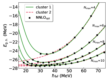
Figure  2 also shows that the data exhibits a simple pattern, namely U-shaped curves that get wider and move closer together as $N_{\rm max}$ increases (See also Fig. 8 for another example.) To capture this behavior with an artificial neural network, we choose a sigmoid as the activation function, i.e. $\sigma(x)=(1+e^{-x})^{-1}$. It is then clear that asymptotic values of large $N_{\rm max}$ either map to zero or to one in the activation function, and this explains why – by design – an asymptotically flat function results in the extrapolation. Indeed, using a ReLu function as the activation function (i.e. $\sigma(x)=\max{(0,x)}$) leads to noisy extrapolation results.

II.2 Data Interpolation and Correlated Loss

Despite the fact that we can easily design a neural network that gives satisfactory accuracy on training data, a good performance on making predictions is not guaranteed for the extrapolation problem. More often than not the loss of the testing data will be much larger than the loss of the training data, which is a clear sign of overfitting. Overfitting is a major issue for neural network applications, which is usually caused by the conflict between having insufficient information from a limited dataset, and the networks flexibility to approximate complex non-linear functions. This is exactly the case for the ab initio extrapolation task at hand. The ab initio calculations are restricted to a not-too-large value of $N_{\rm{max}}$, and for a given $N_{\rm max}$ only a few oscillator spacings $\hbar\omega$ are available. In the case of ⁴He, for instance, we only have 144 data points from NCSM calculations, and this is is inadequate for training even a very simple neural network, thus overfitting seems inevitable.

There are a few strategies that can be introduced to avoid overfitting in neural networks, including regularizations Zou and Hastie (2005), dropout Srivastava et al. (2014), and early stopping Prechelt (1998). Such methods can be used together or separately to increase the network robustness and reduce generalization errors. The price to pay is that one will have to deal with more hyperparameters and determine the best combination of them. Besides these methods, one of the best ways to reduce overfitting is to enlarge the data set. In our case, however, the commonly used practice of data augmentation Tanner and Wong (1987) and addition of random noise to the data set will not be helpful, because extrapolation is a quantitative problem that requires high accuracy and input data with a clear physical foundation.

To enlarge the data set, we note that the ab initio calculations for a given $N_{\rm{max}}$ should give a continuous smooth curve for the target observable values as a function of $\hbar\omega$. The limited input data is merely restricted by the computation cost but not by the method itself. Thus, performing interpolation on existing data is an economical way to obtain more information. In this work, we employ a quadratic spline for interpolation in $\hbar\omega$ at fixed $N_{\rm max}$. This procedure increases the robustness of the neural network even with the basic single-hidden-layer architecture and avoids overfitting.

As a large portion of the training data is generated by interpolation, the standard “$\chi^{2}$” loss function (valid for independent data) might not be appropriate. As the generation of $n$ points via interpolation yields $n$ correlated samples, we introduce the correlated loss function

$$L=\displaystyle\sum_{i=1}^{n}\displaystyle\sum_{j=1}^{n}W_{ij}R_{i}R_{j}.$$ (4)

Here $W_{ij}$ are the elements of a correlation matrix, and $R_{i}$ $(R_{j})$ are the residuals of the $y_{\rm{pre}}$ and the target $y_{\rm{true}}$. In this work, we will either consider the absence of correlations (i.e. $W_{ij}=\delta_{ij}$) or include correlations as described in what follows. The elements $W_{ij}$ form a block matrix, because only points interpolated at fixed $N_{\rm max}$ are correlated by the spline. For fixed $N_{\rm{max}}$ the block matrix is taken to be tridiagonal with all non-zero matrix elements equal to one. This indicates that the correlation is only between neighboring data points. We note that the loss function (4) is usually not a built-in function for much of the mainstream neural network development environments. Thus, we employ a customized loss function, and the position $i$ or $j$ of each data point is needed as an additional input for the network to generate the correlation matrix with elements $W_{ij}$.

Training a neural network starts with a random initialization of the network parameters (weights and biases). During training the loss function is minimized using the training data set as input. It is clear that the random starting points will lead to different trained networks, because optimizers can generally not find the global minimum of the loss function. The existence of many local minima with an acceptable loss will thus lead to different network predictions.

Inspired by the random forest algorithm Breiman (2001), in which the decision forest always gives better performance than a single decision tree, we introduce multiple neural networks with the same structure but with different initialized parameters to address the uncertainty problem. The outputs of all the networks are being integrated in order to obtain a range of predictions and uncertainty estimates. This approach is going to help us to reveal some insights into neural networks, and guide us in selecting favorable neural network solution.

Figure 3 demonstrates the impact of including correlations into the loss function. The left panels shows the predictions of 100 neural networks for the ground-state energy of ⁴He. The input data consists of NCSM data for model spaces with a maximum value of $N_{\rm max}$ as indicated, and the correlation matrix $W$ of Eq. (4) is taken to be diagonal, i.e. no correlations are included. The displayed ground-state energies are the neural network predictions for $N_{\rm max}=100$, and there is virtually no $hw$-dependence. The shown distribution function results from Kernel Density Estimations (KDE), i.e. by replacing the delta-function corresponding to each individual data point with a Gaussian. The distribution becomes narrower as the input data includes increasing values of $N_{\rm max}$. We note that the distributions are bi-modal.

Figure 3: (Color online) Distributions of multiple neural network trained with different max$(N_{\rm{max}})$ datasets for ground-state energy of ⁴He using $\chi^{2}$ loss function (left panel) and correlated loss (right panel).

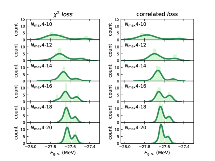
The inclusion of correlations, shown in the right panel of Fig. 3, somewhat reduces the importance of the smaller peak. The main peaks, which include most of the network results, exhibit a smaller average loss and therefore are believed to be the better solution. Their central values are likely the to be the best predictions for these networks. However, for uncorrelated and correlated loss functions, the second peak does not appear by accident and can not be neglected. Its persistence against different optimizers and hyperparameter adjustments shows that it is a stable local minimum and not too narrow. From this point of view, both peaks can be treated as the solutions of the multiple neural networks. As the maximum $N_{\rm{max}}$ of the input data is increased, the two peaks are getting closer to each other but remain distinguishable. Thus, a significant uncertainty remains.

II.3 Multiple Neural Network and Data Preprocessing

We want to understand the bi-modal structure of the distribution functions. For this purpose, we focus on the correlated loss function. Figure 4 presents results from 100 neural networks for the correlated loss versus the ⁴He ground-state energy $E_{\rm{g.s.}}$. Each cross in Fig. 4 represents one fully trained neural network and has already reached convergence (i.e. the loss shift is within a required accuracy). As before, the shown distribution function results from KDE. Each individual data point (crosses) and contour lines are also shown. The top and right panels show the integrated distributions for the ground-state energy and the loss, respectively.

Figure 4: (Color online) Multiple neural network predictions for extrapolating ground-state energy of ⁴He with NCSM calculated dataset max$(N_{\rm{max}})=20$ as input. Kernel density estimations for $E_{\rm{g.s.}}$ and loss are also given along side. The calculation contains 100 independent random initialized neural network.

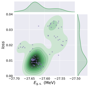
We understand the double-peak structure as follows. The cluster of networks under the dominant peak predict a U-shape for the curves $E_{\rm g.s.}(\hbar\omega,N_{\rm max})$ at fixed $N_{\rm max}$. However they deviate in “higher-order” terms that define the precise shape. The smaller cluster of networks under the small peak predict curves $E_{\rm g.s.}(\hbar\omega,N_{\rm max})$ that increase monotonically as a function of $\hbar\omega$. They have a higher loss. This interpretation is based on the results shown in Fig. 2. Here, the black squares are the input data of ground-state energies for given $\hbar\omega$ and $N_{\rm max}$. The green full lines show predictions from the first cluster of networks under the dominant peak of Fig. 4. In contrast, the red dashed lines are predictions from the second cluster of networks under the smaller peak in Fig. 4. It is evident that the networks of cluster 1 learned the pattern of all data while those of cluster 2 failed to predict the trend of the data points at smaller $\hbar\omega$. How did the neural networks of cluster 2 make this mistake?

Inspection showed that the imbalanced dataset is the root of the problem. Our dataset includes many points at relatively large $\hbar\omega$ values (as we used such ultraviolet converged points for infrared extrapolations in Ref. Forssén et al. (2018)), and the corresponding ground-state energies are also much above the variational minimum and the infinite-space result. In contrast, the data set contains a smaller number of data points at relatively small values of $\hbar\omega$, and the corresponding ground-state energies are much closer to the infinite-space result. Thus, the failure to correctly learn about these “minority” data points yields a relatively small increase of the loss function. With random parameters initialization, once the network reaches a local minimum, the imbalanced dataset will, to a large extent, prevent the optimizer from pulling the network out of it. Furthermore, with the imbalanced training data, the effort of emphasizing the minority data directly conflicts with the idea of reducing overfitting. Some of the common neural network strategies, such as adding a regularization term, will make things worse. In contrast, removing data points at too large values of $\hbar\omega$ from the training data set, or a stronger weighting of data closer to the variational minimum (at fixed $N_{\rm max}$) in the loss function, reduces the number of trained networks that would fall into cluster 2.

Figure 5: (Color online) Distributions of multiple neural network for ground-state energy of ⁴He, with the origin datasets (left panel) and with the preprocessed datasets (right panel).

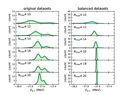
In the ab initio calculation, when the $\hbar\omega$ of the harmonic oscillator basis is too large or too small (i.e. it deviates from the “optimal” value $\hbar\omega\approx{\hbar^{2}\Lambda/(mR)}$, where $\Lambda$ and $R$ are the scales set by the cutoff of the potential and the radius of the computed nucleus Hagen et al. (2010)), the convergence with respect to the increasing $N_{\rm{max}}$ is slow, because the employed basis is not efficient to capture ultraviolet and infrared aspects of the problem. The data points that we are most interested in are close to the variational minimum at fixed $N_{\rm{max}}$. To overcome the problem of the imbalanced dataset, we apply Gaussian weights on the input data, using the values of the minima for the centroids and a standard deviation of about 8.5 MeV. The networks are trained using these weights and a correlated loss function. Figure 5 shows the comparison of multiple neural network results with and without sample weights. We note that the two panels have different ranges for $y$-axis to better display the distribution of the ground-state energy. Training with the original datasets (left panel) yields the bi-modal distribution. Introducing balanced datasets via Gaussian weights (right panel) suppresses the second peak and leaves us with one solution for the extrapolation problem. At the same time, this improves the precision of the predicted observable and thus yields a smaller uncertainty for the neural network extrapolation.

Figure 6: (Color online) Extrapolated results for ⁴He ground-state energy (upper panel) and point-proton radius (lower panel) with NCSM datasets from $\rm{max}(N_{\rm{max}})=10$ to $\rm{max}(N_{\rm{max}})=20$ employing neural network (squares) and IR (circles) extrapolation. Error bars represent the uncertainties of the extrapolations that are due to changes in the initial point in the training process.

We note here that the increased weighting of points close to the variational minima is a akin to employing a prior in Bayesian statistics. Such techniques could also be used for a quantification of uncertainities Schindler and Phillips (2009); Furnstahl et al. (2015); Carlsson et al. (2016); Neufcourt et al. (2018). In this work, we limit ourselves to uncertainty estimates.

III Results and discussions

We now present the results of the neural networks’ predictions for ground-state energies and radii, and compare with other extrapolation methods. We start with the nucleus ⁴He. The networks are trained separately for the ground-state energy and radius. The datasets are generated by NCSM calculations using the NNLO_opt nucleon-nucleon interaction. Since the four-nucleon bound state of ⁴He is already well converged with the maximum model space that NCSM calculation can reach, it is a good case to perform a benchmark and study the performance of the neural network extrapolations. The networks are trained with different datasets which contain the NCSM results from $N_{\rm{max}}=4$ to the given $\rm{max}(N_{\rm{max}})$. For ⁴He, six datasets with $\rm{max}(N_{\rm{max}})=10$ to $\rm{max}(N_{\rm{max}})=20$ are given, providing the neural network with a sequence of mounting information. The extrapolation result for the single neural network is given by the prediction of $N_{\rm{max}}=100$ when the observable value is virtually constant in the interval $10~{}\rm{MeV}<\hbar\omega<60~{}\rm{MeV}$. With each dataset, the multiple neural network (containing 100 networks) is trained with randomly initialized network values. The distribution of the multiple neural network results is then fitted by the Gaussian function. Finally, the recommended values of the multiple neural networks are set to be the mean value $\mu$ and the uncertainties are defined as the standard deviation $\sigma$ of the Gaussian.

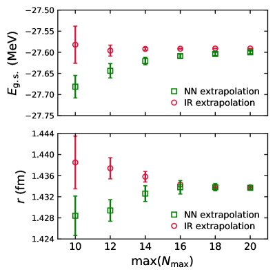
Figure 6 shows the predictions and corresponding uncertainties for the neural network approach compared with the values obtained from the infrared (IR) extrapolations of Ref. Forssén et al. (2018). The error bars reflect the variations that are due to changes in the initial point in the training process. As we can see, the uncertainty of the neural network predictions decreases with increasing $\rm{max}(N_{\rm{max}})$. This indicates that the network is learning the pattern as the data set is enlarged. The neural networks reach convergence after $\rm{max}(N_{\rm{max}})=16$ and their predictions agree with the IR extrapolations for both the ground-state energy and point-proton radius. We note that the two extrapolation methods exhibit different behaviors while reaching identical converged values.

Figure 7: (Color online) Extrapolated results for ⁶Li ground-state energy (upper panel) and point-proton radius (lower panel) with NCSM datasets from $\rm{max}(N_{\rm{max}})=12$ to $\rm{max}(N_{\rm{max}})=22$ employing neural network (squares) and IR (circles) extrapolation. Error bars represent the uncertainties of the extrapolations that are due to changes in the initial point in the training process.

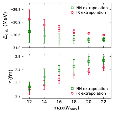
⁶Li is a more challenging task for both $ab~{}initio$ calculations and extrapolations. This is a weakly bound nucleus where a weakly bound deuteron orbits the ⁴He core. Thus, the radius is relatively large, and the calculated observables converge slowly as the model space increases. This nucleus is a good challenge for extrapolation methods. The results for neural network extrapolations are shown in Figure 7. For the ground-state energy, the neural network gives $E_{\rm{g.s.}}=-30.743\pm 0.061~{}\rm{MeV}$ with the largest dataset $\rm{max}(N_{\rm{max}})=22$ and the results start to converge when $\rm{max}(N_{\rm{max}})$ reaches 16. As a long-range operator the radius converges even slower than the energy, which makes it more difficult for the extrapolation method to obtain a reliable prediction. With the largest dataset, the neural network extrapolated result is $r_{\rm{p}}=2.471\pm 0.028~{}\rm{fm}$ and the predictions start to converge at $\rm{max}(N_{\rm{max}})=20$. The error bars reflect the variations that are due to changes in the initial point in the training process.

So far, we have only studied the uncertainties from the random starting point when training the network. To study the robustness of the trained neural networks, we proceed as follows. Once a network is trained, i.e. once its weights and biases $w$ are determined, we take a random vector (with components drawn at random from a Gaussian distribution with zero mean) $\Delta w$ in the space of weights and biases and adjust its length such that the loss function fulfills $L(w+\Delta w)=cL(w)$, with $c=2$ or $c=10$. These values are motivated as follows. For a chi-square distribution with uncorrelated degrees of freedom, $c=2$ would map out the region of one standard deviation. However, our networks are not that simple and network parameters are correlated. For this reason we also consider the case $c=10$. We note that this approach yields uncertainty estimates but not quantified uncertainties. We then use the new network parameters $w+\Delta w$ to predict the observable of interest. Taking 100 random vectors $\Delta w$ for each single network, we compute the variance in the observable of interest, and also record the maximum deviation. The results are shown in Tables 1 and 2 for $c=2$ and $c=10$, respectively. We see that the network is approximately parabolic at its optimal training point (as variances and maximal deviations increase by about a factor $\sqrt{5}$ as we go from $c=2$ to $c=10$. For energies and radii, the networks are robust. For $c=2$ and $c=10$, the network parameters $|\Delta w|/|w|$ change by about one per mill and one percent, respectively. Allowing for a twofold increase of the loss function, the uncertainty from the training of the network does not exceed the uncertainties from the random initial starting points. However, allowing weights and biases to change such that the loss function is increased by a factor of ten, yields larger uncertainties. In this case, the maximum uncertainties from the neural network (when added to the errorbars shown in Fig. 7), would lead the errorbars from the neural network extrapolation to overlap with those from the IR extrapolation. We note finally that the single-layer neural networks we employ are not resilient with regard to dropout. Removing a single node after training of the network on average changes the predictions for energies and radii by almost 20%.

Table 1: Uncertainty analysis of NN extrapolated results for ⁶Li with weights $w+\Delta w$. The random vector $\Delta w$ of weights and biases is adjusted to double the loss function, i.e. $L(w+\Delta w)=2L(w)$. The quantities $\sigma_{E_{\text{g.s.}}}$ and $\sigma_{r}$ are the standard deviation of the new predictions for ground-state energy (in MeV) and point-proton radius (in fm), respectively. $\text{max}(\Delta E_{\text{g.s.}})$ (in MeV) and $\text{max}(\Delta r)$ (in fm) show the maximal deviation between the new predictions and the origin results. $|\Delta w|/|w|$ are the ratio between norms of the weights deviation and the origin weights.

			max($N_{\text{{max}}}$)
	12	14	16	18	20	22
$\sigma_{E_{\text{g.s.}}}$	0.013	0.010	0.009	0.008	0.009	0.006
$\text{max}(\Delta E_{\text{g.s.}})$	0.068	0.049	0.037	0.031	0.032	0.024
$|\Delta w|/|w|$	0.0009	0.0008	0.0008	0.0008	0.0008	0.0008
$\sigma_{r}$	0.0034	0.0038	0.0042	0.0049	0.0054	0.0061
$\text{max}(\Delta r)$	0.0152	0.0176	0.0200	0.0212	0.0233	0.0269
$|\Delta w|/|w|$	0.0050	0.0043	0.0037	0.0042	0.0043	0.0030

Table 2: Same as as Table 1 but for random vectors $\Delta w$ of weights and biases that yield a tenfold increase of the loss function.

			max($N_{\text{{max}}}$)
	12	14	16	18	20	22
$\sigma_{E_{\text{g.s.}}}$	0.037	0.025	0.023	0.020	0.035	0.016
$\text{max}(\Delta E_{\text{g.s.}})$	0.183	0.121	0.098	0.084	0.153	0.066
$|\Delta w|/|w|$	0.0025	0.0023	0.0021	0.0021	0.0023	0.0021
$\sigma_{r}$	0.0093	0.0093	0.0115	0.0139	0.0154	0.0165
$\text{max}(\Delta r)$	0.0415	0.0393	0.0525	0.0635	0.0684	0.0723
$|\Delta w|/|w|$	0.0122	0.0096	0.0105	0.0105	0.0114	0.0090

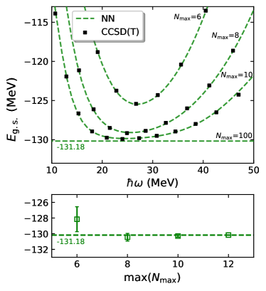
To illustrate the universality of neural network extrapolation, we apply the multiple neural network approach on the ground-state energy of ¹⁶O, computed with the coupled-cluster method Forssén et al. (2018). The upper panel of Fig. 8 shows the neural network performance with the largest datasets [$\rm{max}(N_{\rm{max}})=12$]. As we can see in the lower panel of the figure, the neural network extrapolation results start to converge at $\rm{max}(N_{\rm{max}})=8$. Note that, by then, the neural network is trained with only three sets of $N_{\rm{max}}$ data and still be able to capture the correct pattern. This is due to the quick convergence of the coupled-cluster method itself and the relatively flat curve around the minimum of the energy as a function of $\hbar\omega$, which are both favorable for the neural network extrapolation approach.

Figure 8: (Color online) neural network predictions (upper panel) based on the CCSD(T) dataset with $\rm{max}(N_{\rm{max}})=12$ and multiple neural network extrapolated results (lower panel) with datasets form $\rm{max}(N_{\rm{max}})=6$ to $\rm{max}(N_{\rm{max}})=12$.

IV Summary

In this paper, we presented a neural network extrapolation method to estimate the ground-state energies and point-proton radii from NCSM and the coupled-cluster calculations. To counter the overfitting problem which is caused by the limited set of $ab~{}initio$ results, we enlarged the data set by interpolating between different data points, and used a loss function that accounts for the correlations between the data points. Because of the random nature of the neural network algorithm, we employed multiple neural network approach to obtain recommended results and uncertainties of the extrapolations. We applied balanced sample weights as data preprocessing to eliminate the influences of the persistent local minima, and to obtain a more pronounced single solution for the multiple neural network predictions.

We presented neural-network-extrapolated energies and radii of ⁴He, ⁶Li for NCSM and compared them with IR extrapolated results from Ref. Forssén et al. (2018). The neural network extrapolations gave reliable predictions for both observables with reasonable uncertainties. The extrapolations for the ground-state energy of ¹⁶O from coupled-cluster calculations also yielded accurate results. The strong pattern learning ability of the neural network allowed us to apply the same network architecture for NCSM and CC extrapolation without employing any particular functions. In conclusion, the neural networks studied in this work are useful tools for extrapolating results from ab initio calculations performed in finite model-spaces.