Power-spectrum simulations of radial redshift distributions

Abstract

On the base of the simplest model of a modulation of 3D Gaussian field in $k$-space we produce a set of simulations to bring out the effects of a modulating function $f_{\rm mod}(k)=f_{1}(k)+f_{2}(k)$ on power spectra of radial (shell-like) distributions of cosmological objects, where a model function $f_{1}(k)$ reproduces the smoothed power spectrum of underlying 3D density fluctuations, while $f_{2}(k)$ is a wiggling function imitating the baryon acoustic oscillations (BAO). It is shown that some excess of realizations of simulated radial distributions actually displays quasi-periodical components with periods about a characteristic scale $2\pi/k\sim 100~{}h^{-1}$ Mpc detected as power-spectrum peaks in vicinity of the first maximum of the modulation function $f_{2}(k)$. We revised our previous estimations of the significance of such peaks and found that they were largely overestimated. Thereby quasi-periodical components appearing in some radial distributions of matter are likely to be stochastic (rather than determinative), while the amplitudes of the respective spectral peaks can be quite noticeable. They are partly enhanced by smooth part of the modulating function $f_{1}(k)$ and, to a far lesser extent, by effects of the BAO (i.e. $f_{2}(k)$). The results of the simulations match quite well with statistical properties of the radial distributions of the brightest cluster galaxies (BCGs).

Keywords  methods:statistical – galaxies: distances and redshifts – cosmology: observations – large-scale structure of Universe

1 Introduction

In this paper we consider statistical properties of the radial (shell-like) distributions of matter, that is a set of cosmological objects (characterized by redshifts) observed in various directions in dependence only on their comoving line-of-sight distances. We focus on a study of possible quasi-periodical components in the radial distribution of matter and estimations of their significance. The study of radial distribution of matter inhomogeneities is of special interest to cosmology because its results allow twofold interpretations, either temporal or spatial ones. In particular, the temporal interpretation dominated in literature over long time in the context of possible incorporation of wave processes in the cosmological evolution (e.g., Morikawa 1991; Aref’eva and Koshelev 2008; Hartnett and Hirano 2008; Hirano and Komiya 2010). The spatial interpretation of quasi-periodicities in the radial distributions occurs much less frequently because it assumes some fraction of spatial order at least in some parts of the Universe (e.g., Einasto et al. 1997a, b, 2016).

One can treat our statistical approach as a somewhat different view on well-known statistics. So in our previous papers (e.g., Ryabinkov et al. 2013; Ryabinkov and Kaminker 2014, hereafter Paper I and II) we discussed an appearance of quasi-periodical components in the radial distributions of a few samples of redshifted objects adhering to the spatial interpretation. The reason was that the main scale revealed in these works $\sim 100~{}h^{-1}$ Mpc, where $h=H_{0}/100$ km s^-1 Mpc^-1, $H_{0}$ – the present Hubble constant, was a spatial scale approximately corresponding to the Baryon Acoustic Oscillations (BAO) (e.g., Eisenstein and Hu 1998; Eisenstein et al. 1998a, 2007; Bassett and Hlozek 2010; Percival et al. 2010; Anderson et al. 2012; Kazin et al. 2014; Anderson et al. 2014; Alam et al. 2017; Ross et al. 2017; Vargas-Magaña et al. 2018 and references therein).

It is well-known that the phenomenon of the BAO is the oscillatory dependence of the power spectrum of luminous-matter fluctuations on a wave number $k$. Amplitudes at some $k$ in the Fourier space were enhanced and at others – reduced during the recombination epoch. These enhancements and suppressions manifest itself as quasi-periodical variations imprinted in the power spectrum with the period $2\pi/r_{s}$ corresponding to so called standard “ruler” $r_{s}$. Such oscillations might be superimposed on random fluctuations of density (and velocity) of luminous matter in the subsequent epochs (e.g., Sunyaev and Zeldovich 1970; Peebles and Yu 1970; Zeldovich and Novikov 1983) and in principle could promote the emergence of secondary quasi-periodicities in the radial distribution of the objects.

We proceeded from an assumption that the radial distributions of cosmological objects may exhibit peaks in their power spectra due either to stochastic processes or as footprints of actual periodical components. Here we evaluate significance of such peaks visible in the radial power spectra and estimate probability for the peaks to occur in vicinity of the BAO scale. We consider the simplest model of the Gaussian field modulation in the $k$-space accounting for two factors: (i) a smooth galaxy power spectrum (e.g., Feldman et al. 1994) described by a function $f_{1}(k)$, (ii) damped oscillations of the power spectrum described by a model function $f_{2}(k)$, which is designed with using the approximation of Blake and Glazebrook (2003) to simulate the BAO effect. Our main simplifications are concerned with full disregard of evolutionary effects and a consideration of pure spatial coordinate systems (CS) — Cartesian or spherical ones — conventionally treated in the present time. It makes sense to note that just the evolution can lead to non-linearity and non-Gaussian effects which we do not consider here. We neglect also a velocity field of galaxies.

All spatial coordinates $x,y,z$ as well as coordinates $k_{x},k_{y},k_{z}$ in the Fourier space are measured in cosmological units $h^{-1}$ Mpc and $h$ Mpc^-1, respectively, keeping in mind possible applications of the results to a flat cosmological (comoving) space (e.g., Sect. 4).

Actually, we proceed from the Gaussian mock data in real (comoving) space, produce a modulated random field in the $k$-space and then transform the field back to the real space. This allows us to examine an occurrence of quasi-periodicities in the radial distributions and infer a conclusion about a probability to find those or other spatial periodic components. We consider such components as quasi-periodical because of limited intervals of line-of-sight distances used in all analyzed samples and, as it is shown below, because of the fact that an appearance of such components has stochastic nature in principle and should be described in terms of probabilities.

Our main results are that the BAO modulation can not provide relatively high amplitudes of the peaks in the radial power spectra declared in Papers I and II. Thereby the hypothesis about an impact of the BAO is not confirmed. On the other hand, it is shown that the high amplitudes can be induced by basic fluctuations of 3D power spectrum, which could be treated as a cosmic variance. That strongly reduces significance of the peaks. Note that our new evaluations and our conclusions may be referred to both spatial and temporal interpretation.

In Sect. 2 we determine basic values and definitions used in our simulations. In Sect. 3 we introduce a modulating function $f_{\rm mod}(k)$ and present results of the statistical analysis of simulated radial distributions; in Sect. 4 we compare the results with those obtained in a similar way for samples of spectroscopic redshifts $z$ detected for so-called brightest cluster galaxies (BCGs) or the most luminous galaxies in the clusters. Conclusions and discussions of the results are given in Sect. 5.

2 BASIC DEFINITIONS

We start our simulations in the Cartesian CS and generate homogeneous, isotropic Gaussian mock fields $G(x,y,z)$ as discrete cubic matrices with ${\cal N}_{bin}^{3}$ cells (bins) and the mean M$[G]$ equal to the variance D$[G]$. For certainty we choose M$[G]=$D$[G]=100$.

As the second step we produce a Fourier transform into ${\bf k}$-space for each realization of $G(x,y,z)$ :

$$F_{G}({\bf k})={1\over L^{3}}\,\int\,{\rm d}^{3}{\bf r}\,G({\bf r})\,e^{-i{\bf k}{\bf r}},$$ (1)

where $L={\cal N}_{bin}\Delta_{b}$ is a linear size of a cubic box under investigation, $\Delta_{b}$ is a size of a cell (bin), in this work we put $\Delta_{b}=10~{}h^{-1}$ Mpc. Components of ${\bf k}$ in the Cartesian CS – $k_{x},k_{y},k_{z}$ form also cubic matrices with the same number of bins ${\cal N}_{bin}^{3}$. As a result of Eq. (1) we obtain two 3D-matrices corresponding to real Re$(F_{G})$ and imaginary Im$(F_{G})$ parts of the complex values $F_{G}$. To return back to the real space one can produce an inverse Fourier transform with inclusion of a modulating function $f_{\rm mod}(k)$

$$U({\bf r})={L^{3}\over(2\pi)^{3}}\,\int\,{\rm d}^{3}{\bf k}\,F_{G}({\bf k})\,\sqrt{f_{\rm mod}(k)}\,e^{i{\bf k}{\bf r}},$$ (2)

where $k=\sqrt{k_{x}^{2}+k_{y}^{2}+k_{z}^{2}}$, $U({\bf r})=U(x,y,z)$ is modulated random field which is an original subject of the further statistical simulations.

Following standard definition one can introduce a variance of the modulated field $U({\bf r})$:

$${\rm D}[U]=\frac{\sum_{i}\ \sum_{j}\ \sum_{l}\,(U(x_{i},y_{j},z_{l})-U_{0})^{2}}{{\cal N}_{bin}^{3}-1},$$ (3)

where $U_{0}={\rm M}[U]$ and in our case $U_{0}={\rm M}[G]=100$.

We introduce the normalized 3D random field

$$u({\bf r})={U({\bf r})-U_{0}\over\sqrt{D[G]}}=\sqrt{U_{0}}\ \delta({\bf r}),$$ (4)

where $\delta({\bf r})=[n({\bf r})-n_{0}]/n_{0}$ is a standard density contrast,  $n({\bf r})=U({\bf r})/\Delta_{b}^{3}$ is a number density in different cubic bins with coordinates designated by a radius-vector ${\bf r}$,  $n_{0}=U_{0}/\Delta_{b}^{3}$ is a mean number density over the treated volume. The denominator is selected somewhat artificially by analogy with the Poisson-like statistic, although we have $U_{0}={\rm D}[G]\neq{\rm D}[U]$; this choice will be justified below.

The value $u({\bf r})$ allows to calculate a normalized Fourier transform:

$$F_{u}({\bf k})={1\over L^{3}}\,\int\,{\rm d}^{3}{\bf r}\,u({\bf r})\,e^{-i{\bf k}{\bf r}}={F_{G}({\bf k})\ \sqrt{f_{mod}(k)}\over\sqrt{{\rm D}[G]}},$$ (5)

where the second equality follows from Eqs. (2) and (4) at $k>0$. Then 3D power spectrum is:

$$P_{3D}(k) = \langle|F_{u}(k)|^{2}\rangle_{V_{k}}={1\over V_{k}}\ \int_{V_{k}}\ {\rm d}^{3}{\bf k}^{\prime}\ |F_{u}({\bf k}^{\prime})|^{2}$$ (6)

$$= U_{0}P_{\rm st}(k),$$

where $\langle...\rangle_{V_{k}}$ is averaging over a spherical shell in $k$-space, $V_{k}=4\pi k^{2}\Delta_{k}$ and $\Delta_{k}$ are the volume and the width of the shell, respectively. The integration in Eq. (6) is equivalent to averaging over all possible directions of the vector ${\bf k}$ within the spherical shell $\Delta_{k}$ (e.g., Feldman et al. 1994); $P_{\rm st}(k)=\,\langle|\delta_{\bf k}|^{2}\rangle$ is the standard dimensionless power spectrum, where $\langle...\rangle$ is an ensemble averaging (e.g., Peacock 2003). Using the second equality in Eq. (5) and Parseval’s theorem (e.g., Feldman et al. 1994), applied to the Gaussian field $G$, one can rewrite Eq. (6) as

$$P_{3D}(k)={f_{mod}(k)\over{\rm D}[G]}\ \langle|F_{G}({\bf k})|^{2}\rangle_{V_{k}}\simeq f_{mod}(k).$$ (7)

It makes sense to introduce also a normalized correlation (auto-correlation) function of the isotropic and homogeneous modulated random field $u({\bf r})$:

$$\xi_{3D}(\delta r) = \langle u({\bf r})u({\bf r}\ +\ \delta{\bf r})\rangle_{\rm V}$$ (8)

$$= {L^{3}\over 2\pi^{2}}\,\int{\rm d}k\,k\,{\sin{k\delta r}\over\delta r}\,P_{3D}(k),$$

where $\langle...\rangle_{\rm V}$ – averaging over the normalization volume $V=L^{3}$, typical $\delta r=$ $\sqrt{\delta r_{x}^{2}+\delta r_{y}^{2}+\delta r_{z}^{2}}$ obeys to a condition $\delta r<<L$.

By analogy with straightforward 3D definitions of Eqs.(4)–(8) one can derive also the key quantities for the radial distribution of objects. It is convenient to introduce an arbitrary centre of coordinates ${\bf r}_{0}\,(x_{0},y_{0},z_{0})$, and concentric spherical layers (bins) $r_{b}\pm\Delta_{r}/2$ at the distance $r_{b}$ from the centre, $r_{b}=\sqrt{(x_{b}-x_{0})^{2}+(y_{b}-y_{0})^{2}+(z_{b}-z_{0})^{2}}$, $x_{b},y_{b},z_{b}$ – coordinates of points located in centres of cubic bins constituting a spherical layer, $\Delta_{r}=\Delta_{b}$ is a width of a layer, $\Delta_{b}$ is determined in Eq. (1).

Let us treat the discrete numbers (in each cell of the matrix) defined by the modulated random field $U({\bf r})$, as a sample of statistical points (e.g., galaxies). Then we can calculate a radial distribution function, $N_{R}(r)$, as a number of points inside a concentric non-overlapping bin:

$$N_{R}(r_{b})={1\over\Delta_{b}^{3}}\int_{r_{b}-\Delta_{r}/2}^{r_{b}+\Delta_{r}/2}\,{\rm d}r\,r^{2}\ \int\ {\rm d}\phi\,{\rm d}\theta\,\sin{\theta}\,U({\bf r}),$$ (9)

where $n(r_{b})=N_{R}(r_{b})/4\pi r_{b}^{2}\Delta_{r}$ $\approx n(r)$ is a mean number density within a concentric layer.

In analogy with Eq. (4) we introduce a normalized radial distribution function:

$$u_{R}(r_{b})={N_{R}(r_{b})\,-\,n_{0}\ 4\pi\ r_{b}^{2}\,\Delta_{r}\over\sqrt{n_{0}\ 4\pi\ r_{b}^{2}\,\Delta_{r}}}=\langle u({\bf r})\rangle_{r_{b}}\sqrt{{\cal N}_{r_{b}}},$$ (10)

where $n_{0}\ =\ U_{0}/{\Delta_{b}^{3}}$, $\langle u({\bf r})\rangle_{r_{b}}$ is the normalized random field (4) averaged over the spherical layer; ${\cal N}_{r_{b}}$ is a number of cubic bins inside the spherical shell; at ${\cal N}_{r_{b}}\gg 1$ we have ${\cal N}_{r_{b}}=4\pi r_{b}^{2}\Delta_{r}/\Delta_{b}^{3}$. The difference between Eqs. (4) and (10) is that (4) refers to any points ${\bf r}$ in the considered volume while (10) describes spherical layers around a selected centre.

The radial distributions of real objects (e.g., luminous red galaxies (LRG) discussed in Paper I) display quite complex radial behaviours including large-scale variations or so-called trends. To study specially intermediate scales one needs to reduce an influence of the largest scales or the smallest wave numbers $k$ in the Fourier space. Therefore, in some cases we introduce a trend-subtraction procedure which consists in a replacement of the value $n_{0}4\pi r_{b}^{2}\Delta_{r}$ in Eq. (10) by a smooth trend function $N_{\rm tr}(r_{b})$. Such modified forms of Eq. (10) are specially indicated in the text.

In principle the normalized radial distribution $u_{R}(r_{b})$ can be treated as a 3D-distribution averaged over angles within each shell and with the same variance as $u({\bf r})$ in (4). Actually, it can be shown that ${\rm D}[u_{R}]={\rm D}[u]$. However, here we focus specially on 1D-approach to the radial distribution of $u_{R}(r_{b})$ as more simple way to detect possible variations in spatial distributions of the cosmologically remote objects. Thus we calculate the power spectrum of the normalized radial distribution $u_{R}(r_{b})$ using the one-dimensional definition (e.g., Jenkins and Watts 1969; Scargle 1982)

$$P_{R}(k_{m})=|F_{R}^{1D}(k_{m})|^{2}=$$ (11)

$${1\over{\cal N}_{R,bin}}\left\{\left[\sum_{j=1}^{{\cal N}_{R,bin}}u_{R,j}\cos(k_{m}r_{b,j})\right]^{2}+\right.$$

$$\left.\left[\sum_{j=1}^{{\cal N}_{R,bin}}u_{R,j}\sin(k_{m}r_{b,j})\right]^{2}\right\},$$

where $F_{R}^{1D}(k_{m})=({\cal N}_{R,bin})^{-1/2}\sum_{j=1}^{{\cal N}_{R,bin}}u_{R,j}e^{-ik_{m}r_{b,j}}$ is the one-dimensional discrete Fourier transform, ${\cal N}_{R,bin}$ is a number of concentric bins (shells), $j=1,2,...\ {\cal N}_{R,bin}$ is a numeration of the bins, $r_{b,j}$ is a localization of a centre of $j$-th bin, $k_{m}=2\pi m/L_{R}$ is a wave number corresponding to an integer harmonic number $m=1,2,...{\cal M}$,  ${\cal M}={\cal N}_{R,bin}/2$ is a maximal number (the Nyquist number) of independent discrete harmonics, $L_{R}$ is the whole interval in the configuration space, i.e., so-called sampling length.

The value $P_{R}(k)$ is the key value of our radial approach, where $k$ is conjugate value to the radial distance $r$. Note that the power spectrum (11) differs from the power spectrum $P_{1D}(k_{z})$ of the pencil-beam 1D samples discussed, e.g. by Kaiser and Peacock (1991), because as opposed to a single direction in the case of $P_{1D}(k_{z})$ in (9), (10) we analyze a variety of directions (averaged over the angles) characterized by the single variable $r_{b}$ measured relative to the selected centre.

Following an analogy with Eq. (8), but employing the one-dimensional approach of Eq.(11), and continuing the discrete consideration of Eqs. (9), (10) and (11) we can introduce a value:

$$\xi_{R}(\delta r) = \langle u_{R}(r_{b})\ u_{R}(r_{b}+\delta r)\rangle_{\rm R}$$ (12)

$$= 2\sum_{m=1}^{\cal M}\ P_{R}(k_{m})\,\cos(k_{m}\delta r),$$

where $\delta r$ designates a set of discrete distances between central radii $r_{b,j}$ of concentric layers,  $\langle...\rangle_{\rm R}=\sum_{j=1}^{{\cal N}_{R,bin}}.../{\cal N}_{R,bin}$ is an averaging over all concentric layers consistent with the sampling length $L_{R}$; this is similar to the averaging $\langle...\rangle_{\rm V}$ introduced in Eq. (8) but with central symmetry preservation.

3 MODEL SIMULATIONS

The main goal of this work is to carry out simulations of the modulated Gaussian 3D-fields having a chance to reproduce – with some probability – quasi-oscillations in the radial (shell-like) distributions of cosmological objects.

To trace the modulation effects on properties of the radial distribution of matter we introduce a modulating function $f_{\rm mod}(k)=f_{1}(k)+f_{2}(k)$, where a smooth function $f_{1}(k)$ is designed as

$$f_{1}(k)=f_{\rm CDM}(k)+1,$$ (13)

here $f_{\rm CDM}(k)$ is a power spectrum of the cold dark matter (CDM) density (e.g., Bardeen et al. 1986)

$$f_{\rm CDM}(k)=A_{1}\cdot q\,{\rm T}^{2}(q),$$ (14)

$A_{1}$ is a normalizing constant, $q$ is dimensionless variable $k=|{\bf k}|$ determined according to Sugiyama (1995) as

$$q=\frac{k/({\rm Mpc}^{-1}\ h)}{\Omega_{\rm m}h\exp[-\Omega_{\rm b}(1+\sqrt{2h}/\Omega_{\rm m})]},$$ (15)

where $\Omega_{\rm m}$ is the relative total density of matter, $\Omega_{\rm b}$ is the relative density of baryons, ${\rm T}(q)$ is a transfer function:

$${\rm T}(q)={\ln(1+2.34q)\over 2.34q}\times$$ (16)

$$[1+3.89q+(16.1q)^{2}+(5.46q)^{3}+(6.71q)^{4}]^{-1/4}.$$

The second term “1” in the right side of Eq. (13) stands for so called “shot noise” (e.g., Feldman et al. 1994), which dominates at small scales (large $k$).

The function $f_{2}(k)$ is simulated as a product

$$f_{2}(k)=f_{\rm CDM}(k)\,\cdot f_{\rm BAO}(k),$$ (17)

where $f_{\rm CDM}(k)$ is defined by Eqs. (14)-(16) and $f_{\rm BAO}(k)$ is a damped oscillation function designed as a modification of the fitting formula (3) of Blake and Glazebrook (2003) introduced to imitate the BAOs:

$$f_{\rm BAO}(k)=A_{2}\ {k\over k_{s}}\ \exp\left[-\left({k\over 0.1~{}h~{}{\rm Mpc}^{-1}}\right)^{1.4}\right]\times$$

$$\left[1+\sin\ ({2\pi k\over k_{s}}+\phi_{s})\right],$$ (18)

where $k_{s}=0.0628\ h$ Mpc^-1 or $2\pi/k_{s}=100~{}h^{-1}$ Mpc, $\phi_{s}$ is a phase; below we choose $\phi_{s}=1.4$ to make a position of the main peak of $f_{2}(k)$ equal to $k_{s}$. In what follows one can make sure that the accurate form of Eq. (18) is not important.

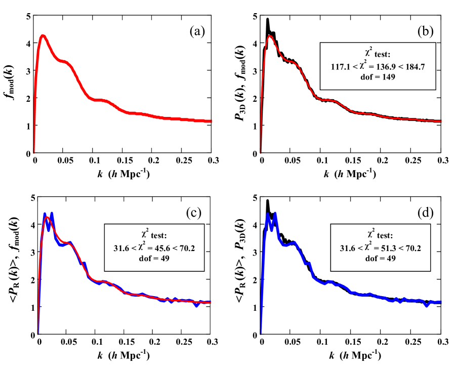
Fig. 1 : (Colour online) Panel (a) $-$ function $f_{\rm mod}=f_{1}(k)+f_{2}(k)$ (solid) used for modulation of the 3D Gaussian field in ${\bf k}$-space, where $f_{1}$ is a model function simulating a smoothed 3D power spectrum [Eq. (13)], $f_{2}$ is a damped oscillating model function [Eq. (17)];  panel (b) $-$ comparison of simulated power spectrum of the 3D Gaussian field $P_{3D}(k)$ (thick wavy curve) [see text] with modulating function $f_{\rm mod}(k)$ (thinner solid curve) ; the insert shows result of $\chi^{2}$ two-sides test calculations for 150 bins along $k$-axis. A simulated quantity of the Pearson sample statistics $\chi^{2}=\chi_{\nu}^{2}$, where $\nu=149$ is a number of degrees-of-freedom (dof), and critical quantiles confining a confidence region (with confidence probability $0.95$) are represented;  panel (c) $-$ comparison of simulated radial power spectrum $\langle P_{R}(k)\rangle$ (thick solid curve) averaged over 500 radial power spectra with modulating function $f_{\rm mod}(k)$ (thinner solid curve); panel (d) $-$ comparison of $P_{3D}(k)$ (same as in panel (b)) with $\langle P_{R}(k)\rangle$ (same as in panel (c));  inserts in the panels (c) and (d) are organized similar to the insert in the panel (b) but for simulations with $\nu=49$ dof.

The modulating function

$$f_{\rm mod}(k)=f_{\rm CDM}(k)\cdot[1+f_{\rm BAO}]+1$$ (19)

is represented in Fig. 1(a). For certainty we put the normalizing constant $A_{1}=470$ as a better approximation to the observational power spectrum (used from Anderson et al. 2014). Note that the functions $f_{1}(k)-1=f_{\rm CDM}(k)$ and $f_{2}(k)$ tend to zero at $k\rightarrow 0$, i.e at very large scales.

Additionally, we introduce $A_{m}(k)=f_{2}(k)/f_{1}(k)$ as a relative amplitude of oscillating modulation in dependence on $k$. In particular, the main peak of the modulating function $f_{2}(k_{s})$ corresponds to $A_{m}=A_{m}(k_{s})=f_{\rm BAO}(k_{s})\cdot f_{\rm CDM}(k_{s})\ [f_{\rm CDM}(k_{s})+1]^{-1}$. To make the effects of the BAO more visible we admit hereafter that $A_{m}=0.2$. It is approximately twice as much as the double observational BAO amplitude ($\approx 2\times 0.05=0.1$, e.g., Blake and Glazebrook 2003,  Anderson et al. 2014). This way we overestimate effects of the oscillating part of the modulation on the radial power spectra.

Employing Eqs. (2), (9) and (10) we produce the modulated random fields in the Cartesian coordinate system (CS) and calculate a set of normalized radial (shell-like) distribution functions $u_{\rm R}(r)$, where $r$ is a distance between coordinates ($x,y,z$) of field points and arbitrary chosen centres (null points) of the radial distributions ${\bf r}_{0}$  ($x_{0},y_{0},z_{0}$). Using Eq. (11) we obtain a sample of radial power spectra $P_{\rm R}(k)$, where $k$ is a variable conjugate to the distance $r$, and carry out a statistical analysis of the sample. The results of such analysis are represented in Figs. 1–4.

So the thick solid curve in Fig. 1(a) displays the modulating function $f_{\rm mod}=f_{1}(k)+f_{2}(k)$ introduced in Eq. (19) to simulate the modulation of the 3D Gaussian field in ${\bf k}$-space. A comparison of simulated 3D power spectrum $P_{3D}(k)$ obtained with using Eq. (6) and the modulating function $f_{\rm mod}(k)$ is represented in Fig. 1(b). The insert shows results of $\chi^{2}$ two-sides test calculations for 150 bins along $k$-axis. In this case we use a definition

$$\chi^{2}=\chi_{\nu}^{2} = \sum_{m=1}^{\cal M}\left({P_{3D}(k_{m})-f_{\rm mod}(k_{m})\over\sigma_{3D}(k_{m})}\right)^{2},$$

$$\sigma_{3D}(k_{m}) = P_{3D}(k_{m})\ N_{m}^{-1/2},$$ (20)

where ${\cal M}$ is the Nyquist number (${\cal M}=150$), $\sigma_{3D}(k_{m})$ is the standard deviation determined for statistics of the mean values, $N_{m}$ is the number of values $P_{3D}(k_{m})$ involved in averaging within a spherical shell (6) $V_{k}=4\pi k_{m}^{2}\Delta_{k}$, i.e., approximately $N_{m}\approx 4\pi(k_{m}/\Delta_{k})^{2}$. Note that the sample length is chosen as $L=3000$ Mpc $h^{-1}$ and $\Delta_{k}=2\pi/L\simeq 0.0021~{}h$ Mpc^-1.

A comparison of simulated radial power spectrum $\langle P_{R}(k)\rangle$ averaged over 500 power spectra calculated for different radial distributions with the modulating function $f_{\rm mod}(k)$ is shown in Fig. 1 (c). The insert also shows the results of $\chi^{2}$ two-sides test calculations but for 50 bins along $k$-axis, in this case we use

$$\chi^{2}=\chi_{\nu}^{2} = \sum_{m=1}^{\cal M}\left({\langle P_{R}(k_{m})\rangle-f_{\rm mod}(k_{m})\over\sigma_{R}(k_{m})}\right)^{2},$$

$$\sigma_{R}(k_{m}) = \langle P_{R}(k_{m})\rangle\ N_{rd}^{-1/2},$$ (21)

where ${\cal M}=50$, $\sigma_{R}(k_{m})$ is the standard deviation determined similar to Eq. (20), $N_{rd}=500$ is the number of radial distributions, here the sample length is $L_{R}=1000$ Mpc $h^{-1}$ and $\Delta_{k}=2\pi/L_{R}\simeq 0.0063~{}h$ Mpc^-1.

Fig. 1 (d) represents a comparison of $P_{3D}(k)$ [same as in the panel (b)] with $\langle P_{R}(k)\rangle$ [same as in the panel (c)]. The results of $\chi^{2}$ two-sides test calculations for 50 bins along $k$-axis are shown in the insert. Carrying out these calculations we use

$$\chi^{2}=\chi_{\nu}^{2} = \sum_{m=1}^{\cal M}\left({\langle P_{R}(k_{m})\rangle-P_{3D}(k_{m})\over\sigma_{sm}(k_{m})}\right)^{2},$$

$$\sigma_{sm}(k_{m}) = \sqrt{\sigma_{3D}(k_{m})^{2}+\sigma_{R}(k_{m})^{2}},$$ (22)

where ${\cal M}=50$, $\sigma_{sm}(k_{m})$ is the total standard deviation determined by Eqs. (20) and (21). Here as in Fig. 1 (c) the sampling length is $L_{R}=1000$ Mpc $h^{-1}$ for simulations of $\langle P_{R}(k)\rangle$ and as in Fig. 1 (b) – $L=3000$ Mpc $h^{-1}$ for simulations of $P_{3D}(k)$. In such a way we use the same bin in $k$-space $\Delta_{k}\simeq 0.0063~{}h$ Mpc^-1 for calculations of $\langle P_{R}(k)\rangle$ and every third bin $\Delta_{k}\simeq 0.0021~{}h$ Mpc^-1 for calculations of $P_{3D}(k)$.

One can see that the results of calculations represented in Fig. 1 do not contradict (with confident probability 0.95) the hypothesis which can be formalized as an asymptotic double equality

$$f_{\rm mod}(k)=P_{3D}(k)=\langle P_{R}(k)\rangle,$$ (23)

where $\langle...\rangle=\langle...\rangle_{ens}$ is an ensemble averaging, i.e. the averaging over a set of respective radial distributions with numerous centres in real space.

The first equality in Eq. (23) is consistent with Eq. (7), the second one can be roughly explained as follows. If we produce additional averaging of the value $|F_{R}^{1D}(k)|^{2}$ given in Eq. (11) over an interval $k-\Delta_{k}/2\leq k\leq k+\Delta_{k}$ in each realization of the normalized random field $u_{R}(r)$ (considering $k$ as a continuous variable) and implement an ensemble averaging in the $k$-space, then we can assume that $\langle\langle|F_{R}^{1D}(k)|^{2}\rangle_{\Delta_{k}}\rangle_{ens}=\langle|F_{R}(k)|^{2}\rangle_{V_{k}}$, where $\langle...\rangle_{V_{k}}$ is determined in Eq. (6) and $F_{R}(k)$ is the 3D Fourier transform of $u_{R}(r)$. In such a case we can expect that $\langle|F_{R}(k)|^{2}\rangle_{V_{k}}=\langle|F_{u}(k)|^{2}\rangle_{V_{k}}$, because both the fields $u_{R}$ and $u$ have zero mean values and the same variance; the last equality brings us back to the Eq. (7). These assumptions have been confirmed by our simulations.

The second equality in Eq. (23) leads to an unexpected consequence, which can be verified. Actually, if we produce ensemble averaging $\langle...\rangle_{ens}$ of Eq. (12), then with using Eq. (23) we get (in the approximation of continuous variables)

$$\langle\xi_{R}(\delta r)\rangle={L\over\pi}\int_{0}^{\infty}{\rm d}k\cos(k\delta r)P_{3D}(k).$$ (24)

Comparing Eqs. (24) and (8) one can finally obtain

$$\langle\xi_{R}(\delta r)\rangle={2\pi\over L^{2}}\ \int_{\delta r}^{\infty}{\rm d}y\ y\ \xi_{3D}(y),$$ (25)

where $\delta r$ is a distance along an arbitrary radial direction.

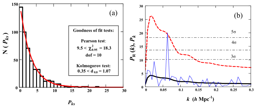
Fig. 2 : Panel (a) $-$ histogram of peak values $P_{ks}$ at fixed $k=k_{s}=0.0628~{}h$ Mpc^-1  obtained for the same 500 radial distributions as in Fig. 1 (c) and (d), within bins $n\leq P_{ks}\leq n+1$, where $n=0,1,2,...,n_{\rm max}$, and compiled with an exponential distribution of peaks (solid line). Insert shows results of Pearson’s $\chi$-square and Kolmogorov’s goodness of fit tests. Panel (b) $-$ power spectrum $P_{R}(k)$ (thin broken curve) calculated for one chosen realization of radial distributions with rather prominent peak near $k_{s}$;  thick solid line – the same modulation function $f_{\rm mod}(k)$ as in Fig. 1 (a), but shown in different vertical scale; thick dashed line is the confidence level $\beta=0.998$ drawn using the mean amplitudes $f_{\rm mod}(k)$ and the exponential distribution function (26); the horizontal thin dot-dashed lines show significance levels estimated according to Scargle (1982) (see text for details).

Our numerous simulations of radial distributions and their power spectra $P_{R}(k)$ have shown that peak height (amplitudes) $P_{k}$ at any fixed $k$ are distributed according to an exponential distribution with the mean (mathematical expectation) peak amplitudes M$[P_{k}]$. In its turn the mean value M$[P_{k}]$ can be determined as the peak amplitude $\langle P_{R}(k)\rangle$ averaged over many centres of radial distributions or, according to Eq. (23), as $f_{\rm mod}(k)$.

Consequently the cumulative distribution function integrating over all values of peak amplitudes $P_{k}$ lower than a fixed value $P^{*}_{k}$ can be expressed as

$${\cal F}(P_{k}<P^{*}_{k},\ \lambda)=1-\exp(-\lambda\ \cdot P^{*}_{k})\,\,\,\,{\rm at}\,\,\,\,P^{*}_{k}\geq 0,$$ (26)

where $\lambda=\lambda(k)$ is a parameter of the exponential distribution determined by a reciprocal modulating function, i.e. $\lambda(k)=f_{\rm mod}^{-1}(k)$. Let us emphasize that the difference between Eq. (13) of Scargle (1982) or Eq. (7) of Frescura et al. (2008) and equation (26) is a constant parameter $\lambda$ of the exponential distributions against a variable $\lambda(k)$ in the present study.

Fig. 2(a) demonstrates a histogram of numbers N$(P_{ks})$ of peak values falling in a bin $n\leq P_{ks}\leq n+1$,  $n=0,1,2,...,n_{\rm max}$, at fixed $k=k_{s}=0.0628~{}h$ Mpc^-1 obtained for the same set of radial distributions as in Fig. 1. The solid line shows theoretical function N${}_{th}(P_{ks})$ of peak amplitudes within each bin at $\lambda(k=k_{s})=1/3.14=0.32$ (where $f_{\rm mod}(k_{s})=3.14$ at $A_{1}=470$) calculated with the use of Eq. (26) following a formula

$${\rm N}_{th}(P_{ks})=[{\cal F}(P_{ks}<n+1)-{\cal F}(P_{ks}<n)]\cdot 500,$$ (27)

where “500” stands for the number of trials.

The insert gives results of two one-side goodness-of-fit tests between the smooth theoretical curve (27) and the histogram: Pearson’s $\chi$-square and Kolmogorov’s tests (e.g., Ledermann and Lloyd 1984). Both the tests demonstrate good agreements at the confidence level 0.95 for $\chi$-square test and 0.8 for the Kolmogorov’s test, the sample size in the former case is $n_{\rm max}=13$ and dof$=13-3=10$ (the number 3 corresponds to the most stringent criterion), while in the latter one the sample volume is $n_{\rm max}=23$; respective quantiles are also indicated in the insert.

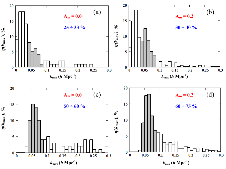
Fig. 3 : Histograms displaying a frequency of occurrence $\eta(k_{\rm max})$  (28) to find the main peak positions $k_{\rm max}$ of radial power spectra within independent bins $\Delta k_{\rm max}=0.01~{}h$ Mpc^-1; dark grey columns indicate regions $0.04\leq k_{\rm max}\leq 0.09~{}h$ Mpc^-1. All four panels are plotted for a sample length $L_{R}=1000~{}h^{-1}$ Mpc;  panels (a) and (c) correspond to the case of zero amplitude $A_{m}=0$ (no BAO effects); panels (b) and (d) – to $A_{m}=0.2$. Approximate fractions (in percents) of peak positions $k_{\rm max}$ falling into the dark grey columns are indicated in all panels. Panels (c) and (d) display effects of a trend subtraction (see text for details) extinguishing Fourier components with $k<0.04~{}h$ Mpc^-1.

Fig. 2(b) demonstrates an example of $P_{R}(k)$ (thin solid curve) calculated using Eq. (11) for one realization of the modulated random field $U({\bf r})$  [Eq. (2)] and, accordingly, of $u_{R}(r)$  [Eq. (10)] at the sampling length $L_{R}=1000~{}h^{-1}$ Mpc (${\cal N}_{R,bin}=100$). One can see a noticeable peak in the power spectra at $k=k_{\rm max}$ which is approximately equal to $k_{s}=0.0628~{}h$ Mpc^-1. The peak corresponds to a scale of quasi-periodicity $\Delta D_{c}=2\pi/k_{\rm max}=L_{R}/m_{\rm max}\simeq 100~{}h^{-1}$ Mpc with $m=m_{\rm max}\simeq 10$.

Employing Eq. (26) we produce estimations of the peak amplitudes $P_{k}$ at a given confidence level $\beta$. The panel (b) demonstrates such a level at $\beta=0.998$ (slightly higher then the Gaussian significance $3\sigma$) for different $k$ (thick dashed curve) together with the mean function $f_{\rm mod}(k)$ (thick solid curve). The horizontal (thin dot-dashed) lines in the panel (b) show the conventional significance levels $3\sigma$ , $4\sigma$, and $5\sigma$ (equivalent to the Gaussian confidence probabilities $\beta=0.998,\ 0.999936,\ 0.9999994$, respectively) calculated for the peak amplitudes $P_{k}$ with the use of the false alarm probability (Scargle 1982,  Frescura et al. 2008). Note that an amplitude of the dominant peak in Fig. 2(b) exceeds the level $5\sigma$ according to Scargle (1982) estimations, but this amplitude turns out to be slightly higher than the level $3\sigma$ estimated using the exponential distribution Eq. (26). In this paper we refer to this more stringent way to estimate the significance of the relatively high peaks ($P_{k}\;\raise 1.29167pt\hbox{$>$\kern-7.5pt\raise-4.73611pt\hbox{$\sim$}}\;20$) in the power spectra which may occur in the modulated Gaussian field.

Fig. 3 demonstrates a frequency of occurrence $\eta(k_{\rm max})$ (in $\%$) of dominate-peak positions $k_{\rm max}$ within different independent bins. This value can be defined as

$$\eta(k_{\rm max})={{\cal N}_{peak}(k_{\rm max})\over{\cal N}_{\rm real}},$$ (28)

where ${\cal N}_{peak}(k_{\rm max})$ is a number of highest peaks falling (independently of their amplitudes) within an interval (bin) $k_{\rm max}^{c}-\ \Delta k_{\rm max}/2\leq k_{\rm max}\leq k_{\rm max}^{c}$ $+\ \Delta k_{\rm max}/2$, $k_{\rm max}^{c}$ is a centre of a bin,  $\Delta k_{\rm max}=0.01$;  ${\cal N}_{\rm real}$ is a full number of realizations (in our case ${\cal N}_{\rm real}=500$); the sampling length is $L_{R}=1000~{}h^{-1}$ Mpc.

Panels (a) and (c) of Fig. 3 correspond to zero value of modulating function $A_{m}=f_{2}(k_{s})/f_{1}(k_{s})$ $=0$ which means zero oscillating component of the modulating function $f_{\rm mod}(k)=f_{1}(k)$, while panels (b) and (d) correspond to $A_{m}=0.2$. Panels (c) and (d) of Fig. 3 display the effects of the trend-subtraction procedure with substitute the value $n_{0}4\pi r_{b}^{2}\Delta_{r}$ in Eq. (10) by a smoothed function (trend) $N_{\rm tr}(r_{b})$ filtering out the largest scales (Fourier components with $k<0.04~{}h$ Mpc^-1). To plot both the histograms in the panels (c) and (d) we calculate the normalized values $u_{R}(r_{b})$ for all partial radial distributions with making use of this procedure. To calculate trend functions $N_{\rm tr}(r_{b})$ we employ the least-squares method with using a set of parabolas. Let us emphasize, however, that the procedure of the trend subtraction is quite ambiguous (e.g., Paper I) and we use it in our simulations only for qualitative consideration.

Dark grey columns in Fig. 3 display fractions of peaks falling into an interval $0.04\leq k_{\rm max}\leq 0.09~{}h$ Mpc^-1 which corresponds to the main bump of the modulation function $f_{2}(k)$ in Fig. 1. Comparing the panels (b) and (a) one can notice a visible excess ($\sim 5-10\%$) of the occurrence $\eta(k_{\rm max})$ at $A_{m}=0.2$ relatively the same value at $A_{m}=0$. Remind that in Fig. 3 we ignore the significance of highest peaks in the radial power spectra being interested only in their positions. Similar moderate gain ($\sim 10-15\%$) in the occurrence of the peaks is noticeable also from a comparison of the panels (d) and (c). On the other hand, an artificial suppression of the smallest $k$ by the trend elimination leads to increase of $\eta(k_{\rm max})$ in the bins belonging to the interval of our interest (cf. panels (c) and (a) at $A_{m}=0$, as well as (d) and (b) at $A_{m}=0.2$). One can notice some pumping of the Fourier components in the nearest regions of $k\;\raise 1.29167pt\hbox{$>$\kern-7.5pt\raise-4.73611pt\hbox{$\sim$}}\;0.04~{}h$ Mpc^-1. In any case, there is enhanced probability to find quasi-periodicities in the radial distributions of matter with a scale $2\pi/k$, where $k$ belongs to the considered interval.

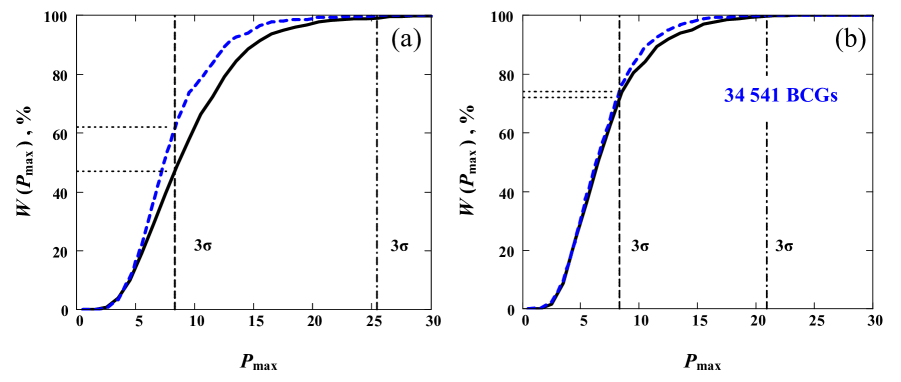
Fig. 4 : (Colour online) Cumulative probability $W(P_{\rm max})=W(P_{k}\leq P_{\rm max})$ to reveal a dominant peak of power spectrum within the interval $0.04\leq k\leq 0.09~{}h$ Mpc^-1 with an amplitude $P_{k}$ not exceeding a fixed value $P_{\rm max}$. The vertical shot dashed lines indicate significance levels $3\sigma$ (slightly higher) corresponding to values $P_{\rm max}$ estimated according to Scargle (1982); the vertical dot-dashed lines show the same significance levels but determined by a condition $W(P_{\rm max})=99.8\%$ (see text); the horizontal short dashed lines show the levels above which significance of the peak exceeds $3\sigma$ (following to Scargle 1982) with probability $1-W(P_{\rm max})$. All curves $W(P_{\rm max})$ refer to the sampling length – $1000~{}h^{-1}$ Mpc. Panel (a) $-$ solid curve corresponds to the amplitude $A_{m}=0.2$, dashed curve $-$ to $A_{m}=0$. Panel (b) $-$ solid curve represents $W(P_{\rm max})$ calculated for 34 541 brightest cluster galaxies (BCGs) (see Sect 4), dashed curve is simulated at $A_{m}=0$ similar to the dashed curve in the panel (a), but produced for a reduced constant $A_{1}^{\prime}=340$ in Eq. (14).

Fig. 4 represents a cumulative probability (in $\%$) $W(P_{\rm max})$ to reveal a dominant peak in the radial power spectrum with an amplitude $P_{k}$ not exceeding a fixed value $P_{\rm max}$ at $k=k_{\rm max}$ falling into the same range $0.04\leq k_{\rm max}\leq 0.09~{}h$ Mpc^-1. This value differs from Eq. (26) by relatively wide range of values $k$ instead of fixed $k$ used in (26). Both the panels in Fig. 4 is plotted for samples of 500 radial power spectra at either $A_{m}=0.0$ or $0.2$ calculated for $k$ from the whole range of $0.0\leq k\leq 0.3~{}h$ Mpc^-1. We evaluate $W(P_{\rm max})$ employing our model simulations or observational data (see below) using natural definition

$$W(P_{\rm max})={{\cal N}(P_{k}\leq P_{\rm max})\over{\cal N}_{\rm real}},$$ (29)

where ${\cal N}(P_{k}\leq P_{\rm max})$ is a full number of realizations with $P_{k}\leq P_{\rm max}$ at fixed $L_{R}=1000~{}h^{-1}$ Mpc.

Fig. 4(a) is obtained without trend-subtraction procedure, i.e. using Eq. (10), as the histograms in Fig. 3(a) and (b), while in Fig. 4(b) the trend-subtraction procedure (see Sect. 4) is included. Our additional simulations show that the curves represented in Fig. 4(a) change insignificantly at filtering out the lowest $k\leq 0.04~{}h$ Mpc^-1.

Vertical dashed lines in both panels of Fig. 4 indicate significance levels $3\sigma$ (slightly higher) corresponding to the value $P_{\rm max}\;\raise 1.29167pt\hbox{$<$\kern-7.5pt\raise-4.73611pt\hbox{$\sim$}}\;10$ calculated following Scargle (1982). Thus in the panel (a) the value $[1-W(P_{\rm max})]$ upward each cross of both curves ($A_{m}=0.2$ and $A_{m}=0$) with the vertical dashed line yields a probability to obtain a peak amplitude exceeding the significance level $3\sigma$. We obtain $38\%$ of all realizations at $A_{m}=0$ and $53\%$ at $A_{m}=0.2$. The excess of the probability $1-W(P_{\rm max})$ at $5<P_{\rm max}\;\raise 1.29167pt\hbox{$<$\kern-7.5pt\raise-4.73611pt\hbox{$\sim$}}\;20$ for the oscillating modulation given by (17) relative to the case $A_{m}=0$ yields an upper limit of difference between the two curves. Let us note, however, that for $P_{\rm max}<10$ and $P_{\rm max}>20$ the solid and dashed curves in Fig. 4 become indistinguishable. Thus the impact of BAO on the most significant peaks are small.

The vertical dot-dashed lines in both panels of Fig. 4 also designate the confidence levels $\beta=0.998$ but calculated from an equality $W(P_{\rm max})=99.8\%$ applied to the solid curves. In addition, one should keep in mind uncertainties of both the curves which make them weakly distinguishable and which we ignore for illustrative purposes.

4 RADIAL DISTRIBUTION OF BCGs

For comparison with real cosmological objects we carry out calculations of the power spectra $P_{\rm R}(k)$ implemented for the radial distributions of brightest cluster galaxies (BCGs). The data on BCGs are based on the data of SDSS catalogue (Wen et al. 2012, Wen and Han 2013). We employ 41 420 most luminous ($M_{r}\leq-23.01$) BCGs within the spectroscopic redshift range $0.044\leq z\leq 0.78$ which corresponds to the comoving-distance range $130.8\leq D_{c}\leq 1956.8~{}h^{-1}$ Mpc. The line-of-sight comoving distances $D_{c}$ are calculated according to the standard expression (e.g., Kayser et al. 1997, Hogg 1999)

$$D_{c}(z_{l})={c\over H_{0}}\ \int_{0}^{z_{l}}\ {1\over\sqrt{\Omega_{\rm m}(1+z)^{3}+\Omega_{\Lambda}}}\ {\rm d}z,$$ (30)

where $l=1,2,...$ numerates redshifts $z_{l}$ of cosmological objects in the sample, $H_{0}$ is defined in Introduction, $c$ is the speed of light; hereafter we use the standard $\Lambda$CDM model with $\Omega_{\rm m}=0.25$ and $\Omega_{\Lambda}=1-\Omega_{\rm m}=0.75$.

We produce a number of radial distributions of the BCGs relative to various reference points (centres), with fixed sample length $L_{\rm R}=1000~{}h^{-1}$ Mpc and using independent bins $\Delta_{c}=10~{}h^{-1}$ Mpc. For this aim we introduce the Cartesian CS employing the data (redshifts $z$ and Equatorial coordinates: right ascension $-$ $\alpha$ and declination $-$ $\delta$) available on the website .

The transformation to the Cartesian coordinates is produced using formulae:

$$X=D_{c}(z)\cdot\sin(90^{\circ}-\delta)\ \cos\alpha$$

$$Y=D_{c}(z)\cdot\sin(90^{\circ}-\delta)\ \sin\alpha$$

$$Z=D_{c}(z)\cdot\cos(90^{\circ}-\delta).$$ (31)

Accordingly, we introduce the distance $r_{l}$ between a point object $(X_{l},Y_{l},Z_{l})$ and a centre of radial distribution $(X_{0},Y_{0},Z_{0})$. It allows us to calculate [employing Eqs. (10) and (11)] $u_{R}(r)$ and $P_{R}(k)$ for any sample of BCGs.

Following two main sky domains of the SDSS data the whole sample of the most luminous BCGs can be subdivided into two subsamples observed in the so-called Northern Galactic Cap (NGC), at $X<0$  (34 541 BCGs) and in the Southern Galactic Cap (SGC), at $X>0$  (6 879 BCGs). Centres of the radial BCG distributions are scattered randomly over two rectangular prisms situated in both galactic hemispheres. For instance, in the case of NGC the boundaries of the prism are (i) $X<0$;   $-1000\leq X_{0}\leq-400~{}h^{-1}$ Mpc, $-500\leq Y_{0}\leq+500~{}h^{-1}$ Mpc, $+100\leq Z_{0}\leq+700~{}h^{-1}$ Mpc.

For either of the two subsamples we produce 500 radial distributions $u_{R}(r)$ and calculate the appropriate radial power spectra $P_{R}(k)$. Then the averaging over all $P_{R}(k)$ yields the mean power spectrum $\langle P_{R}(k)\rangle$. In these calculations we use the trend subtraction procedure described in Sects. 3 to calculate a trend function $N_{\rm tr}(r_{b})$ for each radial distribution. The results of the statistical analysis for the NGC subsample are represented in Figs. 4(b) and 5.

The thick solid curve $W(P_{\rm max})$ in Fig. 4(b) is calculated with the use of Eq. (29) for the sample of 34 541 BCGs. The dashed curve in the same panel represents $W(P_{\rm max})$ obtained in a similar way as the dashed curve in the panel (a) (at $A_{2}=A_{m}=0$) but making use a reduced normalizing constant $A_{1}^{\prime}=340$ in Eq. (14), instead of $A_{1}=470$. That provides a better fit of the $f_{1}(k)$ modulating function to an averaged radial power spectrum $\langle P_{\rm R}(k)\rangle$ produced for the NGC sample. Notice that the two curves (solid and dashed) are close. In particular, it is seen in the panel (b) that the probability $1-W(P_{\rm max})$ for the solid curve to reveal an excess of the peak amplitudes $P_{k}$ over the level $3\sigma$ is $\simeq 28\%$. This is close to $26\%$ for model dashed curve in the same panel. In general, we conclude that the damped oscillations imitating the BAO seems to weakly affect (at any $P_{\rm max}$) the radial power spectra of BCGs.

We verified that the distribution of random peak amplitudes in partial power spectra calculated for either of two BCG subsamples obeys the exponential law, as in the model simulations of Sect. 3, with the parameter $\lambda(k)$ determined by the mean power spectrum $\langle P_{\rm R}(k)\rangle$ at fixed $k$, i.e., $\lambda(k)=\langle P_{\rm R}(k)\rangle^{-1}=f_{1}^{-1}$. Fig. 5(a) represents a histogram of peak values $P_{ks}$ at the same $k=k_{s}=0.0628$ as in Fig. 2(a) and calculated for the same radial distributions of 34 541 BCGs as in Fig. 4(b). The solid line demonstrates theoretical number N($P_{ks}$) of peak amplitudes falling into a bin $n\leq P_{ks}\leq n+1$,   $n=0,1,2,...,n_{\rm max}$. The curve N($P_{ks}$) is obtained using Eq. (27) with $\lambda=1/2.32=0.43$;  $f_{1}(k_{s})=2.32$ at $A_{1}^{\prime}=340$.

As in Fig. 2(a) the insert also gives results of the same one-side goodness-of-fit tests between the smooth theoretical curve (27) and the histogram. Both the tests demonstrate good agreements at the confidence level 0.95 for $\chi$-square test and 0.8 for the Kolmogorov’s test, number of bins in the former case is $n_{\rm max}=10$ and consequently dof $=10-3=7$ (stringent criterion), while in the latter case the sample size is $n_{\rm max}=15$.

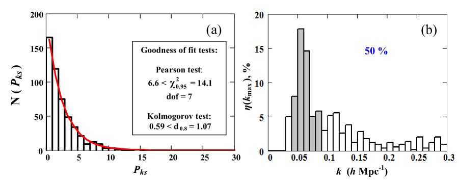
Fig. 5 : (Colour online) Statistical properties of radial power spectra calculated with using (11) for the same sample of 34 541 BCGs as in Fig. 4 (b). Panel (a) is a histogram of peak amplitudes $P_{ks}$ at fixed $k=k_{s}=0.0628~{}h$ Mpc^-1 and theoretical distribution N${}_{th}(P_{ks})$ (solid line) to find a peak amplitude within an interval $n\leq P_{ks}\leq n+1$  ($n=0,1,2,...,n_{\rm max}$), it is similar to Fig. 2 (a);  the insert shows results of Pearson’s $\chi$-square and Kolmogorov’s goodness-of-fit tests;  panel (b) $-$ histogram similar to Fig. 3 (c) and (d).

The panel (b) demonstrates the frequency of occurrence $\eta(k_{\rm max})$ produced in similar way as in the panels (c) and (d) in Fig. 3. One can see that 50$\%$ of the dominate peaks $k_{\rm max}$ occupy the interval $0.04\leq k\leq 0.09$ of our interest. This is consistent with the model histogram at $A_{m}=0$ in Fig. 3(c) with approximately the same probability within the same interval. It also confirms the conclusion about weak influence of the BAO modulation on space distributions of the BCGs.

5 CONCLUSION AND DISCUSSION

The attention of the present paper is payed to the statistical properties of the radial distributions examined as spherically uniform shell-like formations characterized only by a distance from reference points (centres). We consider quasi-periodicities like weak spherical ripples imposed on the matter distribution. The ripples are quite different for different centres (observers) and may be smoothed out by averaging over variety of the radial distributions.

The main results of the present consideration can be summarized as follows.

(1) Properties of the observational 3D-power spectrum of galactic density fluctuations are considered as an origin of quasi-periodicities appearing in the radial distributions of cosmologically remote objects. As a simple test of such a consideration we have implemented simulations of modulated Gaussian fields in the $k$-space. Modulating function for the Gaussian field has been designed as $f_{\rm mod}(k)=f_{1}(k)+f_{2}(k)$ to reproduce a smoothed part of the 3D-power spectrum $-$ $f_{1}(k)$, and to imitate qualitatively the damped oscillations imprinted in the 3D-power spectrum $-$ $f_{2}(k)$. The latter stands for the baryon acoustic oscillations (BAO).

(2) As a result of modulation of the Gaussian field in the Fourier space we obtain radial distributions of cosmological objects in the real space, which may comprise quasi-periodical components displaying themselves as peaks in the radial power spectra and as oscillations of the radial correlation functions (which we do not discuss here). The dominate quasi-periods $\Delta D_{c}=2\pi/k_{\rm max}$ variate mainly around $2\pi/k_{s}$, where $k_{s}$ is a maximum of the first wave (bump) of the modulating function $f_{2}(k)$.

(3) It is shown that the mean radial power spectrum $\langle P_{R}(k)\rangle$  averaged over variety of partial radial power spectra, calculated relatively various centres, turns out to be rather close (in the limit $-$ equal) to the spherically averaged 3D power spectrum (6) produced for the same modulated random field (2). Moreover the modulating function $f_{\rm mod}(k)$ can be formally used as the 3D power spectrum of Gaussian fluctuations (23).

(4) Amplitudes of peaks in the partial radial power spectra are mainly regulated by the smooth modulating function $f_{1}(k)$ and, in a less degree, by a relative amplitude of the first modulating oscillation $A_{m}(k)=f_{2}(k)/f_{1}(k)$ around $k=k_{s}$. Random peak heights at fixed $k$ satisfy the exponential distribution with the exponential parameter $\lambda=\lambda(k)$ determined by the reciprocal modulating function $f_{\rm mod}(k)$. It gives quite simple way to estimate the significance of the peak amplitudes in the radial power spectra. In our result the significance of the dominant peaks at $k_{\rm max}\sim k_{s}$ turns out to be quite moderate ($\;\raise 1.29167pt\hbox{$<$\kern-7.5pt\raise-4.73611pt\hbox{$\sim$}}\;3\sigma$) even for relatively high peak amplitudes $10\;\raise 1.29167pt\hbox{$<$\kern-7.5pt\raise-4.73611pt\hbox{$\sim$}}\;P_{\rm max}\;\raise 1.29167pt\hbox{$<$\kern-7.5pt\raise-4.73611pt\hbox{$\sim$}}\;20$. That means stochastic nature of the appropriate quasi-periodicities.

(5) Probability to obtain the quasi-periodicity in the radial distributions with the spectral peak amplitudes belonging to the interval $10\;\raise 1.29167pt\hbox{$<$\kern-7.5pt\raise-4.73611pt\hbox{$\sim$}}\;P_{\rm max}\;\raise 1.29167pt\hbox{$<$\kern-7.5pt\raise-4.73611pt\hbox{$\sim$}}\;20$ definitely differs for the cases $A_{m}(k_{s})=0.2$ (overestimation of the oscillating component) and $A_{m}(k_{s})=0$ (elimination of this component), but almost indistinguishable and small (a few tenths of a percent) for $P_{\rm max}\;\raise 1.29167pt\hbox{$>$\kern-7.5pt\raise-4.73611pt\hbox{$\sim$}}\;20$. It means that modulation of the Gaussian field by the oscillatory function $f_{2}(k)$ imitating the BAO hardly affects the significance beyond the level $\;\raise 1.29167pt\hbox{$>$\kern-7.5pt\raise-4.73611pt\hbox{$\sim$}}\;3\sigma$.

(6) Results of our simulations of the radial distributions specified by modulated Gaussian fields turn out to be consistent with the results of analysis implemented for radial distributions of the brightest cluster galaxies (BCGs). The radial power spectra calculated for observational data on BCGs and for modulated Gaussian simulations at $A_{m}(k_{s})=0$ (i.e. disregarding the BAO effects) demonstrate mutual consistence of these statistics. This consistence can give an evidence (at least qualitatively) in favour of the model of simple modulation exploited here.

In general, the radial power spectra may display rather strong peaks but estimations of their significance should be implemented by a nonstandard way guided, for instance, by the approach suggested in the present paper.

We carried out additionally another way of statistical averaging of radial distributions produced as numerous realizations of the modulated random field $U({\bf r})$ but simulated relatively to a single centre (ensemble average). Results turned out to be equal to those, described in the present paper, which is obtained with the use of averaging over various centres of the radial distributions but produced for a single realization of $U({\bf r})$ (volume average). We have made sure by simulations that the two considered ways of averaging are equivalent, that is our model simulations do not contradict to the ergodic principle for random fields (e.g., Peacock 2003).

Finally, let us remark that the present work was inspired by a set of papers, e.g., by Kaiser and Peacock (1991), Dekel et al. (1992), Eisenstein et al. (1998b), Yoshida et al. (2001) dedicated to critical examinations of the pencil-beam quasi-periodicity at a scale $\sim$ 130 $h^{-1}$ Mpc found in the pencil-beam surveys near the both Galactic poles by Broadhurst et al. (1990), and confirmed in further studies by Szalay et al. (1991, 1993). Leaving apart the keen question of the significance assessments, the pencil-beam quasi-periodicity can not be referred in a straightforward way to the quasi-periodicity of the radial distributions discussed here. Thus the estimations of the peak significance produced for the distribution of galaxies along pencil beams (inside narrow observational tubes;  e.g., Kaiser and Peacock 1991) noticeably differ from the estimations suggested here for the radial galaxy distributions. However, both types of spatial oscillations despite differences of their scales, in principle, could be related in an indirect way. For instance, there could be different ways to trace the same part of cosmic structure. This set of questions will be touched on by our following paper.

References

- Alam et al. (2017) Alam, S. et al.: Mon. Not. R. Astron. Soc. 470, 2617 (2017)
- Anderson et al. (2012) Anderson, L. et al.: Mon. Not. R. Astron. Soc. 427, 3435 (2012)
- Anderson et al. (2014) Anderson, L. et al.: Mon. Not. R. Astron. Soc. 441, 24 (2014)
- Aref’eva and Koshelev (2008) Aref’eva, I. Ya, Koshelev, A. S.: JHEP 9, 068 (2008)
- Bardeen et al. (1986) Bardeen, J.M., Bond, J.R., Kaiser, N., Szalay, A.S.: Astrophys. J. 304, 15 (1986)
- Bassett and Hlozek (2010) Bassett, B., Hlozek, R.: In: Ruiz-Lapuente, P. (ed.) Baryon acoustic oscillations, p. 246 (2010) arXiv: 0910.5224
- Blake and Glazebrook (2003) Blake, C., Glazebrook, K.: Astrophys. J. 594, 665 (2003)
- Broadhurst et al. (1990) Broadhurst, T.J., Ellis, R.S., Koo, D.C., Szalay, A.S.: Nature 343, 726 (1990)
- Dekel et al. (1992) Dekel, A., Blumenthal, G.R., Primack, J.R., Stanhill, D.: Mon. Not. R. Astron. Soc. 257, 715 (1992)
- Einasto et al. (1997a) Einasto, J. et al.: Mon. Not. R. Astron. Soc. 289, 801 (1997a)
- Einasto et al. (1997b) Einasto, J., Einasto, M., Frisch, P., Gottlober, S., Muller, V., Saar, V., Starobinsky, A.A., Tucker, D.: Mon. Not. R. Astron. Soc. 289, 813 (1997b)
- Einasto et al. (2016) Einasto, J. et al.: Astron. Astrophys. 587, A116 (2016)
- Eisenstein and Hu (1998) Eisenstein, D.J., Hu, W.: Astrophys. J. 496, 605 (1998)
- Eisenstein et al. (1998a) Eisenstein, D.J., Hu, W., Tegmark, M.: Astrophys. J. Lett. 504, 57 (1998a)
- Eisenstein et al. (1998b) Eisenstein, D.J., Hu, W., Silk, J., Szalay, A.S.: Astrophys. J. Lett. 494, 1 (1998b)
- Eisenstein et al. (2007) Eisenstein, D.J., Seo, H.-J., White, M.: Astrophys. J. 664, 660 (2007)
- Feldman et al. (1994) Feldman, H.A., Kaiser, N., Peacock, J.A.: Astrophys. J. 426, 23 (1994)
- Frescura et al. (2008) Frescura, F.A.M., Engelbrecht, C.A., Frank, B.S.: Mon. Not. R. Astron. Soc. 388, 1693 (2008)
- Hartnett and Hirano (2008) Hartnett, J.G., Hirano, K.: Astrophys. Space Sci. 318, 13 (2008)
- Hirano and Komiya (2010) Hirano, K., Komiya, Z.: Phys. Rev. D 82, 103513 (2010).
- Hogg (1999) Hogg, D.W.: astro-ph/9905116 (1999)
- Jenkins and Watts (1969) Jenkins, G.M., Watts, D.G.: Spectral Analysis and Its Applications. Holden-Day Series in Time Series Analysis, London: Holden-Day, 1969
- Kaiser and Peacock (1991) Kaiser, N., Peacock, J.A.: Astrophys. J. 379, 482 (1991).
- Kayser et al. (1997) Kayser, R., Helbig, P., Schramm, T.: Astron. Astrophys. 318, 680 (1997)
- Kazin et al. (2014) Kazin, E.A. et al.: Mon. Not. R. Astron. Soc. 441, 3524 (2014)
- Ledermann and Lloyd (1984) Ledermann, W., Lloyd, E.: Handbook of Applicable Mathematics. Vol. VI: Statistics John Wiley & Sons, New York (1984)
- Morikawa (1991) Morikawa, M.: Astrophys. J. 369, 20 (1991)
- Peacock (2003) Peacock, J.A.: astro-ph/0309240 (2003)
- Peebles and Yu (1970) Peebles, P.J.E., Yu, J.T.: Astrophys. J. 162, 815 (1970)
- Percival et al. (2010) Percival, W.J. et al.: Mon. Not. R. Astron. Soc. 401, 2148 (2010)
- Ross et al. (2017) Ross, A.J. et al.: Mon. Not. R. Astron. Soc. 464, 1168 (2017)
- Ryabinkov et al. (2013) Ryabinkov, A.I., Kaurov, A.A., Kaminker, A.D.: Astrophys. Space Sci. 344, 219 (2013) Paper I
- Ryabinkov and Kaminker (2014) Ryabinkov, A.I., Kaminker, A.D.: Mon. Not. R. Astron. Soc. 440, 2388 (2014) Paper II
- Scargle (1982) Scargle, J.D.: Astrophys. J. 263, 835 (1982)
- Sugiyama (1995) Sugiyama, N.: Astrophys. J. Suppl. Ser. 100, 281 (1995)
- Sunyaev and Zeldovich (1970) Sunyaev, R.A., Zeldovich, Y.B.: Astrophys. Space Sci. 7, 3 (1970)
- Szalay et al. (1991) Szalay, A.S., Ellis, R.S., Koo, D.C., Broadhurst, T.J.: In: Holt, S.S., Bennett, C.L., Trimble, V. (eds.) After the first three minutes. American Institute of Physics Conference Series, vol. 222, p. 261 (1991)
- Szalay et al. (1993) Szalay, A.S., Broadhurst, T.J., Ellman, N., Koo, D.C., Ellis, R.S.: Proc. Natl. Acad. Sci. USA 90, 4853 (1993)
- Vargas-Magaña et al. (2018) Vargas-Magaña, M. et al.: Mon. Not. R. Astron. Soc. 477, 1153 (2018)
- Wen and Han (2013) Wen, Z.L., Han, J.L.: In: Thomas, D., Pasquali, A., Ferreras, I. (eds.) The Intriguing Life of Massive Galaxies. IAU Symposium, vol. 295, p. 188 (2013). 1301.0871
- Wen et al. (2012) Wen, Z.L., Han, J.L., Liu, F.S.: Astrophys. J. Suppl. Ser. 199, 34 (2012)
- Yoshida et al. (2001) Yoshida, N. et al.: Mon. Not. R. Astron. Soc. 325, 803 (2001)
- Zeldovich and Novikov (1983) Zeldovich, I.B., Novikov, I.D.: Relativistic Astrophysics. Volume 2 - The Structure and Evolution of the Universe /revised and Enlarged Edition/. Chicago, IL, University of Chicago Press, 1983, 751 p. Translation. (1983)