Condensate formation and multiscale dynamics in two-dimensional active suspensions

Abstract

The collective effects of microswimmers in active suspensions result in active turbulence, a spatiotemporally chaotic dynamics at mesoscale, which is characterized by the presence of vortices and jets at scales much larger than the characteristic size of the individual active constituents. To describe this dynamics, Navier-Stokes-based one-fluid models driven by small-scale forces have been proposed. Here, we provide a justification of such models for the case of dense suspensions in two dimensions (2d). We subsequently carry out an in-depth numerical study of the properties of one-fluid models as a function of the active driving in view of possible transition scenarios from active turbulence to large-scale pattern, referred to as condensate, formation induced by the classical inverse energy cascade in Newtonian 2d turbulence. Using a one-fluid model it was recently shown (Linkmann et al., Phys. Rev. Lett. (in press)) that two-dimensional active suspensions support two non-equilibrium steady states, one with a condensate and one without, which are separated by a subcritical transition. Here, we report further details on this transition such as hysteresis and discuss a low-dimensional model that describes the main features of the transition through nonlocal-in-scale coupling between the small-scale driving and the condensate.

I Introduction

Active suspensions consist of self-propelled constituents, e.g. bacteria such as Bacillus subtilis and Escherichia coli Wu and Libchaber (2000); Dombrowski et al. (2004), chemically driven colloids Bricard et al. (2013) or active nematics Sanchez et al. (2012); Zhou et al. (2014); Giomi (2015) that move in a solvent liquid, most often water. Their collective motion results in complex patterns on many scales, and shows different phases of coherence and self-organization such as swarming, cluster formation, jets and vortices Dombrowski et al. (2004); Sokolov et al. (2007); Cisneros et al. (2007); Wolgemuth (2008); Wensink et al. (2012); Dunkel et al. (2013a); Gachelin et al. (2014), and, eventually, active or bacterial turbulence Dombrowski et al. (2004). The latter is a state characterized by spatio-temporal chaotic dynamics reminscent of vortex patterns in turbulent flows. The analogy is not complete, though, since Newtonian turbulence is a multiscale phenomenon associated with and dominated by dynamics in an inertial range of scales. Since dissipative effects are negligible in the inertial range, the rate of energy transfer across inertial ranges is constant, and is one of the determining features of the well-known energy cascade Frisch (1995). Thus far, the states that have been described as bacterial turbulence do not have an inertial range.

Active and Newtonian turbulence usually occur in different regions of parameter space. With Reynolds numbers $\mbox{{Re}}=UL/\nu$ based on typical velocities $U$, lengths $L$ and the viscosity $\nu$ of the liquid, one finds turbulence occurs in pipes and other flows for Reynolds numbers around 2000 Landau and Lifshitz (1959); Lautrup ; Avila et al. (2011), while the mesoscale vortices observed in bacterial suspensions Dombrowski et al. (2004) are associated with a Reynolds number of $O(10^{-3}-10^{-2})$, far from the inertial dynamics of Newtonian turbulence. However, rheological measurements of the effective viscosity have shown that the active motion of the constituents can reduce the effective viscosity by about an order of magnitude compared to the solvent viscosity Hatwalne et al. (2004); Liverpool and Marchetti (2006); Sokolov and Aranson (2009); Gachelin et al. (2013); López et al. (2015); Marchetti (2015). Multiscale states at Reynolds number around 30 have been reported for larger microswimmers such as magnetic rotors Kokot et al. (2017). That is, under favorable conditions active suspensions can reach parameter ranges where inertial effects will influence the dynamics, and where a a transition from active to inertial turbulence could be achieved.

The effects of inertia are particularly intriguing in two-dimensional and quasi-two-dimensional suspensions, as kinetic energy is transferred from small to large scales in 2d turbulence, eventually resulting in the accumulation of energy at the largest length scales Kraichnan (1967); Hossain et al. (1983); Smith and Yakhot (1993); Alexakis and Biferale (2018). This phenomenon can be viewed in analogy to Bose-Einstein condensation, which is why the concentration of energy on the largest scales is called the formation of a condensate.

Full models for the dynamics of active suspensions require equations for the velocity field and the swimmers, with suitable couplings between them Liverpool and Marchetti (2008). Since our focus is on the inertial effects in the flow fields, it is advantageous to eliminate the bacteria and to use equations for the flow fields. Such one-fluid models of active suspensions have recently been proposed, Wensink et al. (2012); Słomka and Dunkel (2015) and have already led to a number of numerical investigations into the nonlinear dynamics of active suspensions that have revealed new phenomena, such as nonuniversality of spectral exponents Bratanov et al. (2015), mirror-symmetry breaking Słomka and Dunkel (2017a), or the formation of vortex lattices James et al. (2018). Hints of condensation and multiscaling have been also been observed Oza et al. (2016); Mickelin et al. (2018), but the actual formation of sizeable condensates and the connection between 2d active and Newtonian turbulence have not been explored systematically. Using a variant of these one-fluid models we have recently shown that strong condensates can form in active suspensions, and they do so through a subcritical transition Linkmann et al. (2019). We here provide further results on this transition and on the multiscale dynamics of dense active suspensions.

This paper is organised as follows. We begin with a general discussion of continuum models for active suspensions in Sec. II, including a justification of Navier-Stokes-based one-fluid models for dense suspensions in 2d. Section III contains a description of the datasets collected in direct numerical simulations (DNS), followed by a discussion of the general features of multiscale dynamics and large-scale pattern formation in one-fluid models of active suspensions in Sec. IV. The subcritical transition to condensate formation is described in detail in Sec. V and Sec. VI introduces a low-dimensional model that captures the qualitative features of the transition through a nonlocal-in-scale coupling between the condensate and the driven scales. We summarize our results in Sec. VII.

II Models describing bacterial suspensions

Active suspensions consist of swimmers immersed in a fluid. Models for such suspension have to capture the fluid and the motion of the constituents, which, in a continuum description, leads to a two-fluid approach, where the solvent flow and the coarse-grained motion of the microswimmers are treated as separate but interacting quantities. In order to simplify the models, one-fluid descriptions leading to Navier-Stokes-like equations have been proposed Wensink et al. (2012); Dunkel et al. (2013a, b); Słomka and Dunkel (2015, 2017a). These models usually belong to one of two categories: (i) Bacterial flow models, where the motion of the solvent is eliminated in favor of the bacterial motion Wensink et al. (2012); Dunkel et al. (2013a, b), or, (ii) solvent flow models, where a linear relation between a force on the solvent and the coarse grained motion of the bacteria is postulated Słomka and Dunkel (2015, 2017a). In both cases the resulting velocity field is assumed to be divergence-free, which limits the applicability of these models to very dense suspensions where fluctuations in the bacterial density can be neglected Wensink et al. (2012). In the next subsections, we motivate a single-equation solvent flow model in two dimensions from the general two-fluid approach.

II.1 Justification of effective models in 2d

At the continuum level, an active bacterial suspension can described by equations for the total density $\rho$ and flow velocity ${\bm{u}}$ of the suspension, the concentration $c$ of bacteria and the coarse-grained polarization field ${\bm{p}}$, which plays the dual role of the bacterial velocity and an order parameter for collective phenomena in the bacteria. We assume that the suspension is incompressible, i.e., $\dot{\rho}=0$, implying $\nabla\cdot{\bm{u}}=0$, and that the bacterial concentration is constant, resulting in $\nabla\cdot{\bm{p}}=0$. This then leaves two coupled equations Liverpool and Marchetti (2008), given by

$$\partial_{t}{\bm{u}}+{\bm{u}}\cdot\nabla{\bm{u}} =-\nabla\Pi+\nabla\cdot\sigma^{a}+\nu\Delta{\bm{u}}\ ,$$ (1)

$$\partial_{t}{\bm{p}}+{\bm{u}}\cdot\nabla{\bm{p}} =-\nabla\Pi^{\prime}(|{\bm{p}}|,c)-\lambda_{1}{\bm{p}}\cdot\nabla{\bm{p}}+\frac{1}{2}\bm{\omega}\times{\bm{p}}$$

$$\quad+\lambda\bm{D}\cdot{\bm{p}}+\frac{1}{\gamma_{F}}\bm{h}\ ,$$ (2)

where $\Pi$ is the pressure (divided by the total density) which ensures incompressibility of the velocity field, $\sigma^{a}$ the active stress that couples bacteria and flow (and that will be discussed further below), $\Pi^{\prime}$ is an effective pressure term that depends on the bacterial concentration and the polarization, $\bm{\omega}=\nabla\times{\bm{u}}$ is the vorticity, $\bm{D}=\frac{1}{2}\left[\nabla{\bm{u}}+(\nabla{\bm{u}})^{T}\right]$ the rate of strain tensor, and $\nu$ the kinematic viscosity of the solvent. The parameters $\lambda_{1}$ and $\lambda$ capture advective and flow alignment, and ${{\color[rgb]{0,0,0}\gamma_{F}}}$ is a rotational viscosity.

The molecular field $\bm{h}$ can be obtained from a free energy $F$ for a polar fluid, modelled similar to a liquid crystal, as the derivative, $\bm{h}=-\delta F/\delta{\bm{p}}$, where

$$F=\int\left[\frac{\alpha_{F}}{2}{\bm{p}}^{2}+\frac{\beta_{F}}{4}{\bm{p}}^{4}+\frac{K}{2}(\nabla{\bm{p}})^{2}\right]d{\bm{x}}\ ,$$ (3)

with $K$ the liquid crystalline stiffness in a one-elastic constant approximation and $\alpha_{F}$ and $\beta_{F}$ the parameters which determine the onset of a polarized state for $\alpha_{F}<0$. Note that we have neglected in both equations passive liquid-crystalline stresses of higher order in gradients of the polarization. A derivation of Eq. (II.1) can be found, for instance, in Ref. Liverpool and Marchetti (2008).

The feedback of the active swimmers on the flow is contained in the stress tensors $\sigma^{a}$, which results from the active dipolar forces exerted on the solvent by the microswimmers Simha and Ramaswamy (2002). On length scales large compared to the size of swimmers, it can be expressed through a gradient expansion, with leading order term

$$\sigma^{a(0)}_{ij}=\alpha\left(p_{i}p_{j}-\frac{1}{3}\delta_{ij}{\bm{p}}^{2}\right)+O(\nabla)\ ,$$ (4)

where $\alpha$ is a parameter known as activity, that depends on the concentration of microswimmers, their typical swimming speed and the type of swimmer. The symbol $O(\nabla)$ indicates higher-order terms that contain gradients of the polarization field. The contribution of the diagonal term $-\frac{1}{3}\delta_{ij}{\bm{p}}^{2}$ can be absorbed in the pressure gradient in eq. (1).

Note that the leading-order contribution to the active stress given in eq. (4) has nematic rather than polar symmetry, as it is parity-invariant. Indeed, an active stress with purely polar symmetry arises first in terms containing gradients Giomi et al. (2008), and is given by

$$\sigma^{a(1)}_{ij}=\beta\left(\partial_{i}p_{j}+\partial_{j}p_{i}\right)\ ,$$ (5)

where $\beta$ is another activity parameter that depends, amongst other quantities, on the direction of the polarization field with respect to the swimming direction Liverpool and Marchetti (2008); Baskaran and Marchetti (2009).

In most studies of active suspensions, the fluid flow ${\bm{u}}$ is slaved to the polarization field ${\bm{p}}$, resulting in the Toner-Tu model for the dynamics of the polarization/bacterial velocity Wensink et al. (2012). In contrast, we here wish to eliminate ${\bm{p}}$ in favor of ${\bm{u}}$ in order to obtain an equation for active flows, as done for instance in Ref. Słomka and Dunkel (2017a).

In order to derive such a single-equation model, one has to solve the equation for ${\bm{p}}$ and substitute the solution into the equation for ${\bm{u}}$. Even though the nonlinearities in (II.1) make it difficult to obtain an analytical solution, such an approach will generally give a functional relation between ${\bm{p}}$ and ${\bm{u}}$. In what follows we show how the 2d solvent model can be obtained as the leading-order contribution for the case of a linear, though not necessarily local, relation between ${\bm{p}}$ and ${\bm{u}}$, of the form

$$p_{i}[{\bm{u}}]({\bm{x}},t)=(G_{ij}*u_{j})({\bm{x}},t)\ ,$$ (6)

where $G_{ij}$ is a kernel that depends on the details of the system and $*$ denotes a convolution. The derivation follows similar steps as in active scalar advection in geophysical flows Constantin (1998); Celani et al. (2004).

In 2d, incompressibility of the fields reduces the number of degrees of freedom of each vector field from two to one, usually given by the out-of-plane vorticities $\omega(x,y)=\bm{\hat{z}}\cdot(\nabla\times{\bm{u}}(x,y))$ and $m(x,y)=\bm{\hat{z}}\cdot(\nabla\times{\bm{p}}(x,y))$ of the respective fields, where $\hat{\bm{z}}$ is a unit vector in the $z$-direction. Equation (6) then becomes a scalar relation,

$$m[\omega]({\bm{x}},t)=(G*\omega)({\bm{x}},t)\ .$$ (7)

In a dense bacterial suspension, hydrodynamic interactions are screened and the relation between $m$ and $\omega$ is expected to be local. We can then assume $G$ to be a sharply peaked function, for instance proportional to a narrow spherically symmetric 2d Gaussian

$$G({\bm{x}})=\frac{A}{\pi a}e^{-|{\bm{x}}|^{2}/a^{2}}\ ,$$ (8)

with shape parameter $a>0$ and constant amplitude $A$. Expanding the Fourier transform of the Gaussian in terms of its shape parameter around zero leads to an expansion of eq. (7) of the form

$$m[\omega]({\bm{x}},t)=A\omega({\bm{x}},t)+A\frac{a^{2}}{4}\Delta\omega({\bm{x}},t)+O((a^{2}\Delta)^{2})\ ,$$ (9)

where $\Delta$ the Laplace operator. Since $\nabla\times\omega\bm{\hat{z}}=-\Delta{\bm{u}}$ and similarly for ${\bm{p}}$ and $m$, we obtain

$${\bm{p}}=A{\bm{u}}({\bm{x}},t)+A\frac{a^{2}}{4}\Delta{\bm{u}}({\bm{x}},t)+O((a^{2}\Delta)^{2})\ .$$ (10)

Inserting Eq. (10) into Eq. (4) for the zeroth-order term yields

$$\sigma^{a(0)}_{ij} =\alpha A^{2}\left(u_{i}u_{j}-\frac{1}{3}\delta_{ij}{\bm{u}}^{2}\right){{\color[rgb]{0,0,0}+\alpha A^{2}{a^{2}\over 4}\left(u_{i}\Delta u_{j}+u_{j}\Delta u_{i}\right)}}$$

$$+\alpha A^{2}\frac{a^{4}}{16}\left(\Delta u_{i}\Delta u_{j}-\frac{1}{3}\delta_{ij}(\Delta{\bm{u}})^{2}\right)+O((a^{2}\Delta)^{4})\ ,$$ (11)

resulting in additional quadratic nonlinearities in Eq. (1), some of which break Galilean invariance. The first term in eq. (11) leads to a renormalisation of the Navier-Stokes nonlinearity and hence to a different Reynolds number. Since the sign of $\alpha$ depends on the type of swimmer with $\alpha<0$ for pullers and $\alpha>0$ for pushers, the renormalisation of the Reynolds number depends on the type of microswimmers. The second term can be subsumed into the pressure gradient, while remaining terms which are of higher order in the gradients contribute to a redistribution of kinetic energy mostly at small scales. Since all terms conserve the mean kinetic energy and hence do not result in a net energy input, we neglect the additional small-scale nonlinearities, thereby ensuring Galilean invariance. The energy input from the microswimmers hence has to originate from the first-order term in the gradient expansion of the active stresses given in Eq. (5). Substituting Eq. (10) in Eq. (5) results in

$$\sigma^{a(1)}_{ij} =\beta A\left(1+\frac{a^{2}}{4}\Delta+\frac{a^{4}}{32}\Delta^{2}\right)\left(\partial_{i}u_{j}+\partial_{j}u_{i}\right)$$

$$+O((a^{2}\Delta)^{3})\ ,$$ (12)

where terms up to order $\Delta^{2}$ from Eq. (10) have been included based on stability considerations, and the structure of $\nabla\cdot\sigma^{a(1)}$ takes on the form of the effective viscosity previously proposed by Słomka and Dunkel Słomka and Dunkel (2015), provided $\beta>0$. The latter is the case if ${\bm{p}}$ is chosen to point along the swimming direction and does not depend on the type of microswimmer Baskaran and Marchetti (2009). If we choose ${\bm{p}}$ to point against the swimming direction, then $A$ should be negative. That is, the product $\beta A$ is always positive. In what follows we choose $A>0$ such that ${\bm{p}}$ points into the same direction as the solvent flow. After the rescaling

$$t\to t\sqrt{1-\alpha A},\quad{\bm{u}}\to{\bm{u}}\sqrt{1-\alpha A},$$ (13)

the resulting two-dimensional one-fluid model reads

$$\partial_{t}{\bm{u}}+{\bm{u}}\cdot\nabla{\bm{u}} =-\nabla\Pi+\Gamma\left(\Gamma_{0}+\Gamma_{2}\Delta+\frac{\Gamma_{2}^{2}}{2}\Delta^{2}\right)\Delta{\bm{u}}\ ,$$

$$\nabla\cdot{\bm{u}} =0\ ,$$ (14)

where

$$\Gamma=\frac{\beta A}{\sqrt{1-\alpha A}},\quad\Gamma_{0}=1+\frac{\nu}{\beta A},\quad\Gamma_{2}=\frac{a^{2}}{4}\ .$$ (15)

Equation (II.1) relies upon two main assumptions: (i) ${\bm{u}}$ and ${\bm{p}}$ are divergence-free, i.e. the bacterial concentration must be constant and density fluctuations negligible; (ii) the system must be two-dimensional, as the reduction to a one-dimensional problem resulting in Eq. (7) is not justified otherwise. Specifically, in three dimensions there is no a-priori reason to set $G_{ij}=G\delta_{ij}$ in Eq. (6). In summary, Eq. (II.1) is applicable to dense suspensions of microswimmers in very thin layers, where a 2d-approximation is justified. We note that friction with a substrate has been neglected, however, the corresponding term can easily be added.

In this context, the original introduction of the solvent model by Słomka and Dunkel corresponds to setting $G({\bm{x}})\sim\delta({\bm{x}})$ and using certain higher-order terms in the gradient expansion of the active stresses. The former amounts to assuming that the polarization and solvent velocity fields are related only locally and the latter introduces additional parameters. Physically, locally means on scales smaller than that of the mesoscale vortices. Here, we obtain a very similar model from a long-range relation between the fields, which is more appropriate in a hydrodynamic context.

Similarly, the bacterial flow model introduced in Ref. Wensink et al. (2012) can be obtained by formally solving Eq. (1) to obtain ${\bm{u}}[{\bm{p}}]$, or by neglecting ${\bm{u}}$ altogether. Both solvent and bacterial flow models reproduce the experimentally observed spatiotemporally chaotic dynamics characteristic of active matter turbulence Wensink et al. (2012); Dunkel et al. (2013a); Słomka and Dunkel (2017a) and have been used extensively in investigations thereof Dunkel et al. (2013b); Bratanov et al. (2015); Oza et al. (2016); Słomka and Dunkel (2015); Srivastava et al. (2016); Putzig et al. (2016); Słomka and Dunkel (2017a, b); Doostmohammadi et al. (2017); James and Wilczek (2018); James et al. (2018); Mickelin et al. (2018). They differ in the choice of fields in which the model is expressed, with the consequence that terms originating from the free energy are not explicitly present in the solvent model.

The solvent models resemble the Navier-Stokes equations in their structure and have the key ingredient for an inertial range that is typical of normal turbulence: in the absence of forcing and dissipation, the nonlinear terms in the equation preserve the mean kinetic energy $\langle|{\bm{u}}|^{2}\rangle$. We note that in general Galilean invariance is broken by active corrections coming from Eq. (11) to the advective nonlinearity in Eq. (II.1) that have been neglected here. The effects of the active particles are thus concentrated in the effective viscosity in Eq. (II.1), and we will focus on two variants of the models and discuss similarities and differences to results in the literature that were obtained with the bacterial flow model.

II.2 Polynomial effective viscosity

The solvent model introduced by Słomka and Dunkel Słomka and Dunkel (2015) has a stress tensor in Eq. (1) given by a polynomial gradient expansion

$$\sigma_{ij}=\left(\Gamma_{0}+\Gamma_{2}\Delta+\Gamma_{4}\Delta^{2}\right)\left(\partial_{i}u_{j}+\partial_{j}u_{i}\right)\,,$$ (16)

and results in a continuous effective viscosity

$$\hat{\nu}(k)=\Gamma_{0}-\Gamma_{2}k^{2}+\Gamma_{4}k^{4}\,.$$ (17)

where $\hat{\cdot}$ denotes the Fourier transform. In what follows, we will therefore refer to the combination of Eqs. (1) and (16) as the polynomial effective viscosity (PEV) model.

If $\Gamma_{2}<0$, then Eq. (17) is a combination of normal and hyperviscosity and all terms dissipate energy. If, in contrast, $\Gamma_{2}>0$, there is a wave number interval where $\hat{\nu}(k)<0$, resulting in a linear amplification of the Fourier modes in that wave number interval. The interplay between this instability and the Navier-Stokes nonlinearity drives spatiotemporal dynamics that for certain values of $\Gamma_{i}$ resemble the experimental observations Słomka and Dunkel (2017a).

By completing the square, the wave number form of the effective viscosity can be written as

$$\hat{\nu}(k)=\Gamma_{0}+\Gamma_{4}\left(\left(k^{2}-k_{\rm f}^{2}\right)^{2}-k_{\rm f}^{4}\right)$$ (18)

with

$$k_{\rm f}^{2}=\Gamma_{2}/(2\Gamma_{4})$$ (19)

the wave number of the minimum in the viscosity (which is real only for $\Gamma_{2}>0$). With the normalization of wave numbers to $k_{\rm f}$, i.e. $\tilde{k}=k/k_{\rm f}$, the effective viscosity can be written

$$\hat{\nu}(k)=\Gamma_{0}\left(1+\gamma\left(\left(\tilde{k}^{2}-1\right)^{2}-1\right)\right)$$ (20)

where

$$\gamma=\Gamma_{4}k_{\rm f}^{4}/\Gamma_{0}=\frac{\Gamma_{2}^{2}}{4\Gamma_{0}\Gamma_{4}}=\frac{(\Gamma_{2}/\Gamma_{0})^{2}}{4(\Gamma_{4}/\Gamma_{0})}$$ (21)

is the one remaining parameter that controls the forcing.

The scaled effective viscosity $\hat{\nu}$ has two parameters, $\Gamma_{0}$, which sets the scale for the viscosity, and $\gamma$, which is a measure for both the amplification and the range of wave numbers that are forced, as we will now discuss. The effective viscosity attains its minimum at $\tilde{k}^{2}=1$, where

$$\hat{\nu}(\tilde{k}=1)=\Gamma_{0}(1-\gamma)$$ (22)

Clearly, $\hat{\nu}$ can become negative, and hence forcing rather than dissipating, for $\gamma_{c}>1$ only. The range of wavenumbers over which it is forcing is given by

$$\tilde{k}_{\rm min}^{2}=1-\sqrt{1-\frac{1}{\gamma}}<\tilde{k}^{2}<1+\sqrt{1-\frac{1}{\gamma}}=\tilde{k}_{\rm max}^{2}\ ,$$ (23)

and varies with $\gamma$. A sketch of $\hat{\nu}(k)$ for the PEV model is provided in the top panel of Fig. 1, the gray-shaded area indicating the wavenumber interval where amplification occurs, $\hat{\nu}(k)<0$. The upper end of the interval approaches $2$ for $\gamma\rightarrow\infty$, showing that there will be no forcing on smaller wavelengths, whereas the lower end of the interval approaches $0$, indicating that the driving band extends to ever lower wave numbers and thus larger scales in this limit.

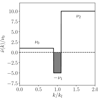
Figure 1: Effective viscosity for PEV and PCV models. Top: PEV $\hat{\nu}/\Gamma_{0}$ vs $k/k_{\rm f}$, bottom: PCV $\hat{\nu}(k)/\nu_{0}$ vs $k/k_{\rm f}$ . The gray-shaded area corresponds to the interval $[k_{\rm min},k_{\rm max}]$, where the amplification occurs.

Since the effective viscosity is measured in units of $\Gamma_{0}$ and since the length scale has been fixed as $L_{\rm f}=\pi/k_{\rm f}$ all scales in the momentum equation are set: specifically, time is measured in units of $L_{\rm f}^{2}/\Gamma_{0}$ and velocity in units of $\Gamma_{0}/L_{\rm f}$. Introducing that scale, Eq. (1) contains a single parameter $\gamma$, with the stress tensor is given by

$$\sigma_{ij}=\left(1+\gamma\left((1+\Delta)^{2}-1\right)\right)\left(\partial_{i}u_{j}+\partial_{j}u_{i}\right)\ .$$ (24)

Variations in $\gamma$ should therefore give rise to different dynamics. Słomka and Dunkel Słomka and Dunkel (2015) discuss statistically steady states for several values of their control parameters $\Gamma_{0}$, $\Gamma_{2}$, and $\Gamma_{4}$, that is, in our notation for different values of $\gamma$ and corresponding driving scales and amplitudes. Some of these states were multiscale with energy spectra reminiscent of fully developed 2d turbulence Słomka and Dunkel (2015); Mickelin et al. (2018), and small condensates were observed for certain parameter values Mickelin et al. (2018). One can then expect that stronger large-scale structures may form for more intense driving, but since $\gamma$ controls not only the strength of the forcing but also the width and the location of the driving band, it is is difficult to see which of the effects dominate. This was remedied in the model used in Linkmann et al. (2019) and described next, where amplification and driving scale can be set independently from each other.

II.3 Piecewise constant viscosity

The piecewise constant viscosity (PCV) model Linkmann et al. (2019) is a discontinuous approximation to the PEV model, with the Navier-Stokes stress tensor written in terms of an effective viscosity given as a set of step functions in Fourier space

$$\hat{\nu}(k)=\begin{cases}\nu_{0}>0\quad\text{for}\quad k<k_{\rm min}\ ,\\ -\nu_{1}<0\quad\text{for}\quad k_{\rm min}\leqslant k\leqslant k_{\rm max}\ ,\\ \nu_{2}>0\quad\text{for}\quad k>k_{\rm max}\ .\end{cases}$$ (25)

The values of $\nu_{i}$ are chosen such that the resulting discrete form of $\hat{\nu}(k)$ resembles the polynomial form of the PEV model. Specifically, $\nu_{1}$ controls the forcing, and $\nu_{2}>\nu_{0}$ mimics the hyperviscous term in the PEV model. A sketch of $\hat{\nu}(k)$ for the PCV model is provided in the bottom panel of Fig. 1, the gray-shaded area indicating the wavenumber interval where amplification occurs, $\hat{\nu}(k)=-\nu_{1}<0$. As in the PEV model, $\nu_{0}$ sets the scale for the effective viscosity. The PCV model can thus be described by dimensionless parameters for amplification, $\nu_{1}/\nu_{0}$, and small-scale dissipation, $\nu_{2}/\nu_{0}$. An effective driving scale $L_{\rm f}=\pi/k_{\rm f}$ can be defined by the midpoint of the interval $[k_{\rm min},k_{\rm max}]$, i.e. $k_{\rm f}=(k_{\rm min}+k_{\rm max})/2$.

Run id	$N$	$\Gamma_{2}/\Gamma_{0}$	$\Gamma_{4}/\Gamma_{0}$	$k_{\rm min}$	$k_{\rm max}$	Re	$U$	$L$	Ref	$\varepsilon_{\rm LS}$	$\varepsilon_{\rm IN}$	$\varepsilon_{\rm SS}$
PEV-1	256	0.002	$7.7\times 10^{-7}$	26	43	14	0.10	0.15	5	0.0012	0.002	0.0008
PEV-2	256	0.0023	$9.3\times 10^{-7}$	23	45	68	0.22	0.35	9	0.0044	0.0072	0.0028
PEV-3	256	0.0025	$9.7\times 10^{-7}$	22	45	668	0.66	1.56	10	0.0097	0.0155	0.0056
Run id	$N$	$\nu_{1}/\nu_{0}$	$\nu_{2}/\nu_{0}$	$k_{\rm min}$	$k_{\rm max}$	Re	$U$	$L$	Ref	$\varepsilon_{\rm LS}$	$\varepsilon_{\rm IN}$	$\varepsilon_{\rm SS}$
PCV-A1∗	256	0.25	10.0	33	40	19	0.29	0.07	19	0.029	0.048	0.023
PCV-A2∗	256	0.5	10.0	33	40	26	0.36	0.085	21	0.056	0.10	0.046
PCV-A3∗	256	0.75	10.0	33	40	35	0.39	0.09	21	0.086	0.16	0.071
PCV-A4∗	256	1.0	10.0	33	40	44	0.43	0.11	21	0.11	0.21	0.09
PCV-A5∗	256	1.25	10.0	33	40	58	0.47	0.13	21	0.15	0.26	0.14
PCV-A6∗	256	1.5	10.0	33	40	75	0.52	0.15	20	0.18	0.30	0.16
PCV-A7∗	256	1.75	10.0	33	40	106	0.57	0.20	19	0.17	0.34	0.16
PCV-A7a	256	1.75	10.0	33	40	106	0.57	0.20	20	0.18	0.32	0.15
PCV-A8∗	256	2.0	10.0	33	40	212	0.66	0.35	19	0.18	0.36	0.18
PCV-A8a	256	2.0	10.0	33	40	227	0.67	0.37	19	0.19	0.34	0.17
PCV-A9∗	256	2.02	10.0	33	40	249	0.68	0.40	19	0.18	0.36	0.18
PCV-A9a	256	2.02	10.0	33	40	2686	1.64	1.79	17	0.15	0.28	0.13
PCV-A10∗	256	2.04	10.0	33	40	296	0.70	0.46	19	0.18	0.36	0.18
PCV-A10a	256	2.04	10.0	33	40	2957	1.77	1.82	17	0.14	0.28	0.13
PCV-A11∗	256	2.083	10.0	33	40	3347	1.95	1.87	17	0.13	0.28	0.15
PCV-A11a	256	2.083	10.0	33	40	3270	1.92	1.85	17	0.14	0.28	0.13
PCV-A12∗	256	2.167	10.0	33	40	3708	2.13	1.90	16	0.13	0.27	0.15
PCV-A13∗	256	2.25	10.0	33	40	3927	2.24	1.91	16	0.13	0.28	0.15
PCV-A14∗	256	2.5	10.0	33	40	4455	2.52	1.92	15	0.12	0.27	0.15
PCV-A15∗	256	2.625	10.0	33	40	4636	2.63	1.92	14	0.11	0.26	0.15
PCV-A16∗	256	2.75	10.0	33	40	4851	2.75	1.92	14	0.11	0.26	0.15
PCV-A17∗	256	2.875	10.0	33	40	5088	2.89	1.92	14	0.11	0.27	0.16
PCV-A18∗	256	3.0	10.0	33	40	5313	3.01	1.92	14	0.11	0.28	0.17
PCV-A19∗	256	3.25	10.0	33	40	5793	3.28	1.92	14	0.12	0.29	0.18
PCV-A20∗	256	3.5	10.0	33	40	6241	3.54	1.92	14	0.13	0.31	0.19
PCV-A21∗	256	3.75	10.0	33	40	6708	3.80	1.93	14	0.13	0.33	0.20
PCV-A22∗	256	4.0	10.0	33	40	7214	4.08	1.93	14	0.14	0.35	0.22
PCV-A23∗	256	4.25	10.0	33	40	7723	4.27	1.93	14	0.16	0.38	0.24
PCV-A24∗	256	4.5	10.0	33	40	8230	4.65	1.93	14	0.17	0.40	0.25
PCV-A25∗	256	4.75	10.0	33	40	8751	4.95	1.93	14	0.18	0.43	0.27
PCV-A26∗	256	5.0	10.0	33	40	9258	5.24	1.93	14	0.19	0.46	0.29
PCV-A27	256	5.25	10.0	33	40	9690	5.51	1.92	15	0.21	0.53	0.32
PCV-A28∗	256	5.5	10.0	33	40	10286	5.81	1.93	15	0.23	0.57	0.34
PCV-A29∗	256	6.0	10.0	33	40	11416	6.44	1.93	15	0.27	0.65	0.39
PCV-A30∗	256	6.5	10.0	33	40	12530	7.08	1.93	15	0.31	0.74	0.44
PCV-A31∗	256	7.0	10.0	33	40	13677	7.77	1.93	16	0.36	0.84	0.49
PCV-B1∗	1024	1.0	10.0	129	160	45	0.027	0.029	21	0.0001	0.00019	9 $\times 10^{-5}$
PCV-B2∗	1024	2.0	10.0	129	160	226	0.041	0.094	20	0.00017	0.00033	0.00016
PCV-B3∗	1024	5.0	10.0	129	160	132914	1.17	1.93	15	0.00018	0.00046	0.00026

Table 1: Parameters and observables for all simulations, with $N$ denoting the number of grid points in each coordinate of the simulation domain $[0,2\pi]^{2}$, $\nu_{0}$, $\nu_{1}$ and $\nu_{2}$, are the parameters defining the PCV-model as in Eq. (25) with $\nu_{0}=0.0011$ for PCV-A and $\nu_{0}=1.7\times 10^{-5}$ for PCV-B. For PEV, the model parameters in Eq. (18) are $\Gamma_{0}=0.0011$, $\Gamma_{2}/\Gamma_{0}$ and $\Gamma_{4}/\Gamma_{0}$. The driven intervals are specified by $k_{\rm min}$ and $k_{\rm max}$ as defined in Eq. (25) for PCV and in Eq. (23) for PEV. The Reynolds number ${\rm Re}$ is based on the integral scale $L=2/U^{2}\int_{0}^{\infty}dk\ E(k)/k$ and the rms velocity $U$, and Re_f is the Reynolds number based on the effective driving scale $L_{\rm f}$ and the velocity in the driven range of scales, $\varepsilon_{\rm LS}$ the energy dissipation rate in the interval $[1,k_{\rm min})$, $\varepsilon_{\rm IN}$ the energy input rate in the interval $[k_{\rm min},k_{\rm max}]$, and $\varepsilon_{\rm SS}$ the energy dissipation rate in the interval $(k_{\rm max},2\pi/(N/3)]$. All observables are ensemble-averaged during the statistically stationary state, with samples taken at intervals of one large-eddy turnover time $T=L/U$. The asterisk indicates data from Ref. Linkmann et al. (2019).

The PCV model approximates the functional form of the PEV model’s effective viscosity by a piecewise constant function, remaining faithful to the original PEV model in an important point: The driving is proportional to the velocity field and it is confined to a wavenumber band. This results in driving through local-in-scale amplification in both cases, i.e. in essentially the same physics. That is, even though the small-scale properties of the velocity fields obtained by the PCV and the original PEV model may differ in some detail, the large-scale and mean properties should be similar, if not the same, as they are dominated by the nonlinearity and not by details of how the driven interval is specified.

III Direct numerical simulations

The PEV and PCV models are studied in two dimensions, using data generated by numerical integration of the momentum equation in vorticity form

$$\partial_{t}\hat{\omega}(\bm{k})+\widehat{\left[\bm{u}\cdot\nabla\omega\right]}({\bm{k}})=-\hat{\nu}(k)k^{2}\hat{\omega}(\bm{k})\ ,$$ (26)

where $\omega$ is the only non-vanishing component of the vorticity, $\nabla\times\bm{u}(x,y)=\omega(x,y)\hat{\bm{z}}$. Equation (26) is supplemented with either Eq. (18) for PEV or Eq. (25) for the PCV model. In all cases, we use the standard pseudospectral technique Orszag (1969) on the domain $[0,2\pi]^{2}$ with periodic boundary conditions and full dealiasing by truncation following the 2/3rds rule Orszag (1971). The simulations are initialised with random Gaussian-distributed data, or, in case of hysteresis calculations for the PCV model, with data obtained from another run at a different value of the control parameter.

The PEV model is only investigated for a small number of test cases corresponding to the parameters specified in table 1. For PCV, two series of simulations were carried out. The first one, PCV-A, consists of a parameter scan in $\nu_{1}/\nu_{0}$ with all other parameters, i.e. $\nu_{0}$, $\nu_{2}$, $k_{\rm min}$ and $k_{\rm max}$ held fixed. That is, only the amplification is varied between the simulations in each PCV-A dataset. The three simulations of the second series, PCV-B, were done at higher resolution, with parameters chosen such that results can be compared with PCV-A using the scaling properties of the Navier Stokes equations, i.e. PCV-B corresponds to PCV-A in a larger simulation domain.Parameters and observables of all runs are summarised in table 1.

All simulations reach a statistically stationary state, where the total energy per unit volume fluctutates about a mean value, and are subsequently continued for at least 2000 large eddy turnover times. Prior to that, the system evolves through a transient non-stationary stage. Owing to the absence of a large-scale dissipation mechanism, this can take a long time for certain parameter regimes. During the statistically stationary state, the velocity fields were sampled in intervals of one large-eddy turnover time.

IV Model dynamics

We begin our study of the properties of the models by tracking the time evolution of the total kinetic energy per unit volume, $E(t)$, given by the difference between input and dissipation,

$$\frac{dE}{dt}=\varepsilon_{\rm IN}(t)-(\varepsilon_{\rm LS}(t)+\varepsilon_{\rm SS}(t))\ ,$$ (27)

where the input $\varepsilon_{\rm IN}$, the large-scale dissipation $\varepsilon_{\rm LS}$ and the small-scale dissipation $\varepsilon_{\rm SS}$ are obtained by integrating the effective viscosity over the piecewise constant intervals, i.e. calculated as

$$\varepsilon_{\rm IN}(t) =-\nu_{1}\int_{k_{\rm min}}^{k_{\rm max}}dk\int d\hat{\bm{k}}|\hat{\bm{u}}(\bm{k},t)|^{2}\ ,$$ (28)

$$\varepsilon_{\rm LS}(t) =\nu_{0}\int_{0}^{k_{\rm min}}dk\int d\hat{\bm{k}}|\hat{\bm{u}}(\bm{k},t)|^{2}\ ,$$ (29)

$$\varepsilon_{\rm SS}(t) =\nu_{2}\int_{k_{\rm max}}^{\infty}dk\int d\hat{\bm{k}}|\hat{\bm{u}}(\bm{k},t)|^{2}\ ,$$ (30)

with $\hat{\bm{k}}=\bm{k}/k$ a unit vector in direction of $\bm{k}$. During statistically stationary evolution, mean energy input must equal mean energy dissipation, $\varepsilon_{\rm IN}=\varepsilon=\varepsilon_{\rm LS}+\varepsilon_{\rm SS}$. The characteristics of the non-stationary evolution depends on the presence of an inverse energy transfer. If an inverse cascade is present, as in fully developed 2d turbulence, it can be expected that $E(t)$ grows linearly in time as long as $\varepsilon_{\rm LS}$ is negligible. This is a consequence of the fact that the dynamics at the small scales are much faster than at large scales leading to $\varepsilon_{\rm IN}\simeq const$ and $\varepsilon_{\rm SS}\simeq const$, and one obtains

$$E(t)\simeq(\varepsilon_{\rm IN}-\varepsilon_{\rm SS})t\ ,$$ (31)

until $\varepsilon_{\rm LS}$ becomes sufficiently large.

The time evolution of the total energy per unit volume, $E(t)$, is shown in Fig. 2 for representative cases. In the top panel, we show the results for the runs PCV-B1, PCV-B2 and PCV-B3 with amplification factors $\nu_{1}/\nu_{0}=1$, $\nu_{1}/\nu_{0}=2$ and $\nu_{1}/\nu_{0}=5$, respectively. The lower frame shows the corresponding results for PEV with parameters $\Gamma_{2}/\Gamma_{0}=0.0025$, $\Gamma_{2}/\Gamma_{0}=0.0023$, and $\Gamma_{2}/\Gamma_{0}=0.002$, with $\Gamma_{4}$ chosen such that the forcing remains centered around $k_{\rm f}=36$.

The behavior of $E(t)$ is qualitatively similar for the two models and differs between the respective example cases. The two cases with low amplification, that is, $\nu_{1}/\nu_{0}=1$ and $\nu_{1}/\nu_{0}=2$ for PCV and $\Gamma_{2}/\Gamma_{0}=0.002$ and $\Gamma_{2}/\Gamma_{0}=0.0023$ for PEV become statistically stationary and fluctuate around relatively low mean values of $E$. In contrast, for the cases $\nu_{1}/\nu_{0}=5$ for PCV and $\Gamma_{2}/\Gamma_{0}=0.0025$ for PEV, the kinetic energy grows at first linearly, which is characteristic of a non-stationary inverse energy cascade in 2d turbulence Boffetta and Ecke (2014). This is followed by statistically stationary evolution, where $E(t)$ fluctuates about mean values which are an order of magnitude larger than for the aforementioned cases. In absence of a large-scale friction term, once an inverse energy transfer is established, statistical stationarity can only be realized through the development of a condensate at the largest scales.

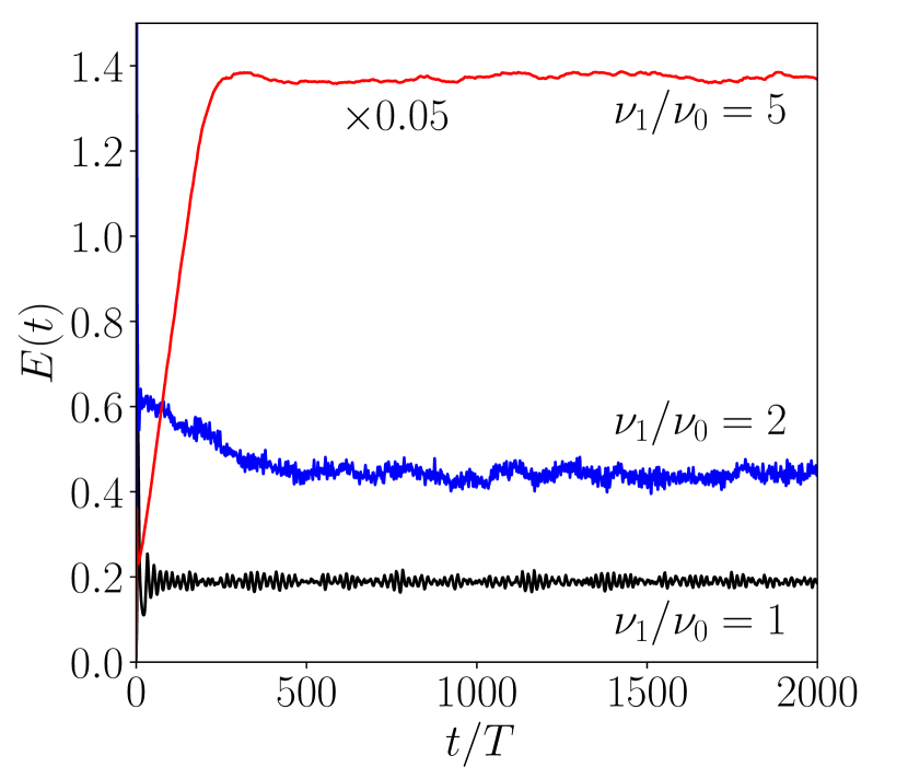
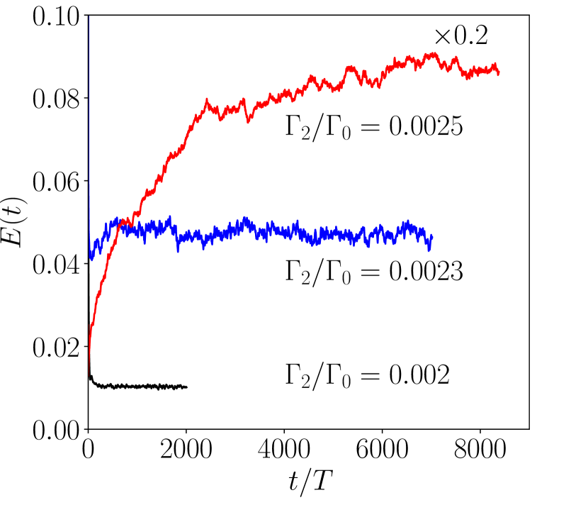
Figure 2: (Color online) Time evolution of the total kinetic energy per unit volume for three example cases for PCV (top) and PEV (bottom). The energy has been divided by a factor of 20 for the PCV case $\nu_{1}/\nu_{0}=5$ and by a factor of 5 for the PEV case $\Gamma_{2}/\Gamma_{0}=0.0025$ in order to improve the readability of the figure.

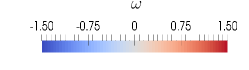
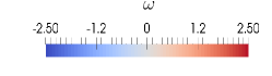
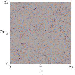
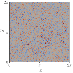
$\nu_{1}/\nu_{0}=1$                                     $\nu_{1}/\nu_{0}=2$                                     $\nu_{1}/\nu_{0}=5$

Figure 3: (Color online) Visualisation of the vorticity field $\omega(x,y)\hat{\bm{z}}$ for PCV cases $\nu_{1}/\nu_{0}=1$ , $\nu_{1}/\nu_{0}=2$ and $\nu_{1}/\nu_{0}=5$ (from left to right) using samples taken during the statistically stationary state.

IV.1 Emergence of large-scale structures

The formation of successively larger structures and the eventual formation of a condensate with increasing amplification can be seen in visualisations of the velocity field, as given in Linkmann et al. (2019). Here, we provide visualisations of $\omega$ for the three PCV cases in Fig. 3. The vorticity fields for $\nu_{1}/\nu_{0}=1$ and $\nu_{1}/\nu_{0}=2$ are similar, with the vortices in the latter case slightly stronger and a bit larger. Finally, for $\nu_{1}/\nu_{0}=5$ a condensate manifests itself in form of two counter-rotating vortices as in classical 2d turbulence Smith and Yakhot (1993); Boffetta and Ecke (2014).

The emergence of large-scale organization and coherence can be quantified through the calculation of equal-time correlation functions. Owing to isotropy, it is sufficient to consider the two-point longitudinal correlator

$${{\color[rgb]{0,0,0}C_{LL}(r)=\langle u_{L}(\bm{x}+\bm{r})u_{L}(\bm{x})\rangle\ ,}}$$ (32)

where $r=|\bm{r}|$, and $u_{L}=\bm{u}\cdot\bm{r}/r$ is the velocity component along the displacement vector $\bm{r}$, and the angled brackets denote a combined spatial and temporal average. Longitudinal correlation functions have been calculated through the spectral expansions of the respective velocity fields for PCV and PEV, with results shown in Fig. 4, where PCV and PEV data are contained in the top and bottom panels, respectively. Clear correlations up to the size of the system can be identified for $\nu_{1}/\nu_{0}=5$ and $\Gamma_{2}/\Gamma_{0}=0.0025$, while $C_{LL}$ decreases much faster in $r$ for the cases without a condensate, $\nu_{1}/\nu_{0}=1$, $\nu_{1}/\nu_{0}=2$, $\Gamma_{2}/\Gamma_{0}=0.002$ and $\Gamma_{2}/\Gamma_{0}=0.0023$.

The differences in correlation can also be quantified with the integral scale

$$L\equiv\frac{1}{{{\color[rgb]{0,0,0}C_{LL}(0)}}}\int_{0}^{\infty}dr\ C_{LL}(r)\ ,$$ (33)

listed in table 1: There is at least an $O(10)$ difference between the respective values of $L$ for PCV-B3 and the two cases with less amplification, PCV-B1 and PCV-B2, and similarly for PEV.

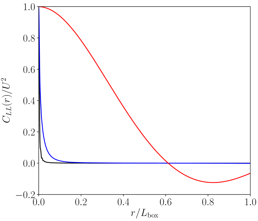
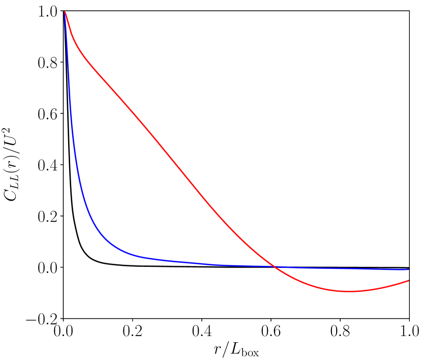
Figure 4: (Color online) Longitudinal correlation functions. Top: PCV for different values of $\nu_{1}/\nu_{0}$. Bottom: PEV for different values of $\Gamma_{2}/\Gamma_{0}$.

V Transition

The transition between the two cases $\nu_{1}/\nu_{0}=1$ and $\nu_{1}/\nu_{0}=2$ without a condensate and $\nu_{1}/\nu_{0}=5$ with a condensate is discontinuous, as shown in Linkmann et al. (2019),

The discontinuous transition between spatiotemporal chaos and classical 2d-turbulence suggests that the two states are separated by a subcritical bifurcation. Accordingly, we expect to find a bistable scenario with the possibility of coexisting states in a parameter range around the transition, and eventually also hysteresis. As observable we take the energy at the largest scale, $E_{1}$, which will be considered as a function of the amplification factor and the energy input. $E_{1}$ is calculated in terms of the energy spectrum

$$E(k)\equiv\left\langle\frac{1}{2}\int d\hat{\bm{k}}\ |\hat{\bm{u}}(\bm{k})|^{2}\right\rangle_{t}\ ,$$ (34)

where $\int d\hat{\bm{k}}$ indicates an average over all angles in $k$-space with prescribed $|\bm{k}|=k$ and $\langle\cdot\rangle_{t}$ denotes a time average. $E_{1}$ is then given by $E_{1}=E(k)_{|k=1}$. Following our analysis in Ref. Linkmann et al. (2019), Fig. 5 presents $E_{1}$ as a function of $\nu_{1}/\nu_{0}$ close to the critical point. Two main features of the transition can be identified in the figure. First, $E_{1}$ increases suddenly at the critical value $\nu_{1}/\nu_{0}=2.00\pm 0.02$, as observed in Ref. Linkmann et al. (2019). Second, the system shows hysteretic behavior: The red (gray) curve consists of data points obtained for decreasing $\nu_{1}/\nu_{0}$, while the black curve corresponds to states obtained for increasing $\nu_{1}/\nu_{0}$. The resulting hysteresis loop is clearly visible.

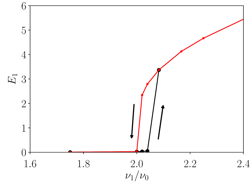
Figure 5: $E_{1}$ as a function of $\nu_{1}/\nu_{0}$. The black curve corresponds to flow states obtained by increasing $\nu_{1}/\nu_{0}$ and the red (gray) curve to flow states obtained by decreasing $\nu_{1}/\nu_{0}$. A hysteresis loop is visible in the region $2.00\leqslant\nu_{1}/\nu_{0}\leqslant 2.04$.

Apart from the presence of hysteresis shown here, the expected bistable scenario is realised in the statistically stationary total energy balance,

$$\varepsilon=\varepsilon_{\rm IN}\simeq 2\nu_{0}\frac{(2\pi)^{2}}{L_{f}^{2}}E_{\rm IN}\ ,$$ (35)

where

$$E_{\rm IN}=\int_{k_{\rm min}}^{k_{\rm max}}dk\ E(k)\ ,$$ (36)

with an upper and a lower branch of $\varepsilon$ as a function of $E_{\rm IN}$ corresponding to classical 2d turbulence with an emerging condensate and spatiotemporal chaos at the forcing scale, respectively, Linkmann et al. (2019). The two branches were found to be connected by an unstable S-shaped region. The existence of two branches connected by an S-shaped region is also visible in the phase-space projection relating the energy at the largest scale to the energy input, i.e. for $E_{1}$ as a function of $\varepsilon_{\rm IN}$ as shown in the top panel of Fig. 6. The lower branch corresponds to injection rates obtained for $\nu_{1}/\nu_{0}<\nu_{1,\rm crit}/\nu_{0}$, where $E_{1}$ is negligible and the inverse transfer is damped by dissipation at intermediate scales before reaching the largest scale in the system. On the upper branch that describes states with a sizeable condensate, we observe a linear relation between $E_{1}$ and $\varepsilon_{\rm IN}$, as can be expected if most energy is dissipated in the condensate

$$\varepsilon_{\rm IN}=\varepsilon\simeq 2\nu_{0}E_{1}k_{1}^{2}\Delta k\ ,$$ (37)

where $k_{1}=1$ is the lowest wavenumber in the domain, and $\Delta k=1$ the width of the wavenumber shell centered at $k_{1}$.

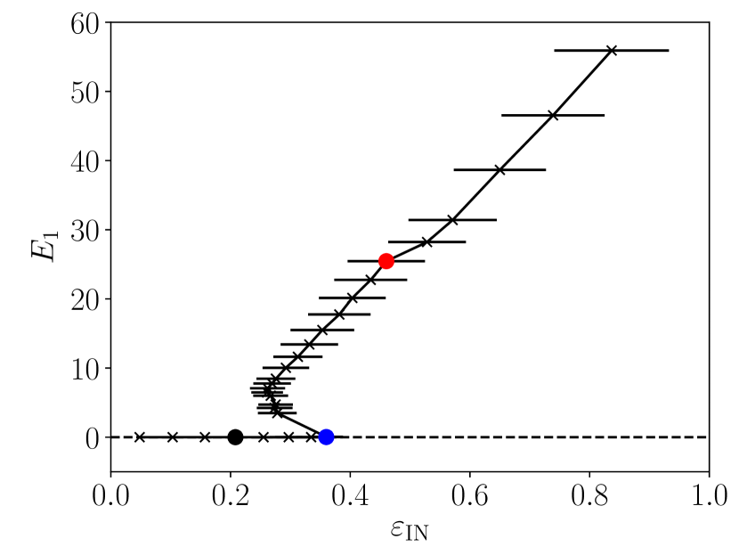
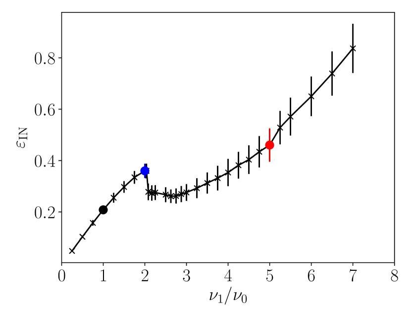
Figure 6: (Color online) Top: $E_{1}$ as a function of $\varepsilon_{\rm IN}$. Bottom: $\varepsilon_{\rm IN}$ as a function of $\nu_{1}/\nu_{0}$. The red (light gray), blue (dark gray) and black dots correspond to the PCV cases discussed in Sec. IV.

The S-shaped region in the top panel of Fig. 6 can only occur if $\varepsilon_{\rm IN}$ is a non-monotonous function of the amplification factor. This is indeed the case as can be seen in the bottom panel of the same figure, where a sudden decrease in $\varepsilon_{\rm IN}$ occurs at $\nu_{1,\rm crit}/\nu_{0}$, followed by an interval in $\nu_{1}/\nu_{0}$ where $\varepsilon_{\rm IN}$ varies very little. Eventually, for states with a strong condensate $\varepsilon_{\rm IN}$ increases linearly with $\nu_{1}/\nu_{0}$. The nature of the transition is thus related to non-monotonous behavior of the energy input (and therefore the dissipation) as a function of the control parameter, which can only occur if the energy input depends on the velocity field. In particular, for Gaussian-distributed and $\delta$-in-time correlated forcing $\varepsilon_{\rm IN}$ itself is the control parameter and a scenario as described here is unlikely to occur. This observation suggests that the type of transition depends on the type of forcing, that is, it is non-universal.

As explained in Sec. II.2, the structure of the PEV model make a parameter study with fixed energy input range difficult. However, the nature of the transition is unlikely to be affected by the simplifications made in the PCV model, as the PEV and PCV models have the same structure in the sense that energy input is given by linear amplification. The PEV simulations also show a sudden formation of a condensate under small changes in the amplification as can be seen from the comparison of correlation functions in the bottom panel of Fig. 4.

To compare to experimental data and between the two models, we define a Reynolds number based on the effective driving scale, $L_{\rm f}$ and the velocity at the driven scales

$${\rm Re}_{f}=\frac{\sqrt{E_{\rm IN}}L_{\rm f}}{\tilde{\nu}}\ ,$$ (38)

where $\tilde{\nu}$ is the Newtonian viscosity, i.e. $\tilde{\nu}=\nu_{0}$ for PCV and $\tilde{\nu}=\Gamma_{0}$ for PEV. This Reynolds number corresponds to the Reynolds number associated with the mesoscale vortices observed in experiments. Values of ${\rm Re}_{f}$ for all simulations are given in table 1. The transition occurs at ${\rm Re}_{f}\simeq 20$ for PCV and at ${\rm Re}_{f}\simeq 10$ for PEV, the exact value may depend on simulation details such at the width of the driving range and the level of small-scale dissipation. However, the main point is that both models transition at Reynolds number of $O(10)$. In comparison, the experimentally observed Reynolds numbers are about $O(10^{-2})$, based on characteristic vortex sizes of $100\mu m$, with a characteristic speed of $100\mu m/s$ for B. subtilis Dombrowski et al. (2004), and the kinematic viscosity of water $\nu_{\rm H_{2}O}=10^{-6}(\mu m)^{2}/s$.

V.1 Spectral scaling

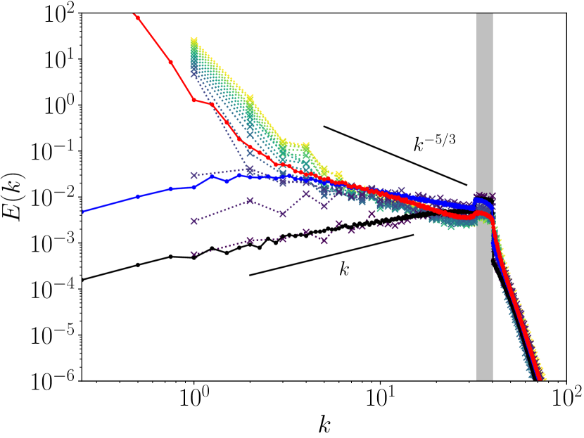
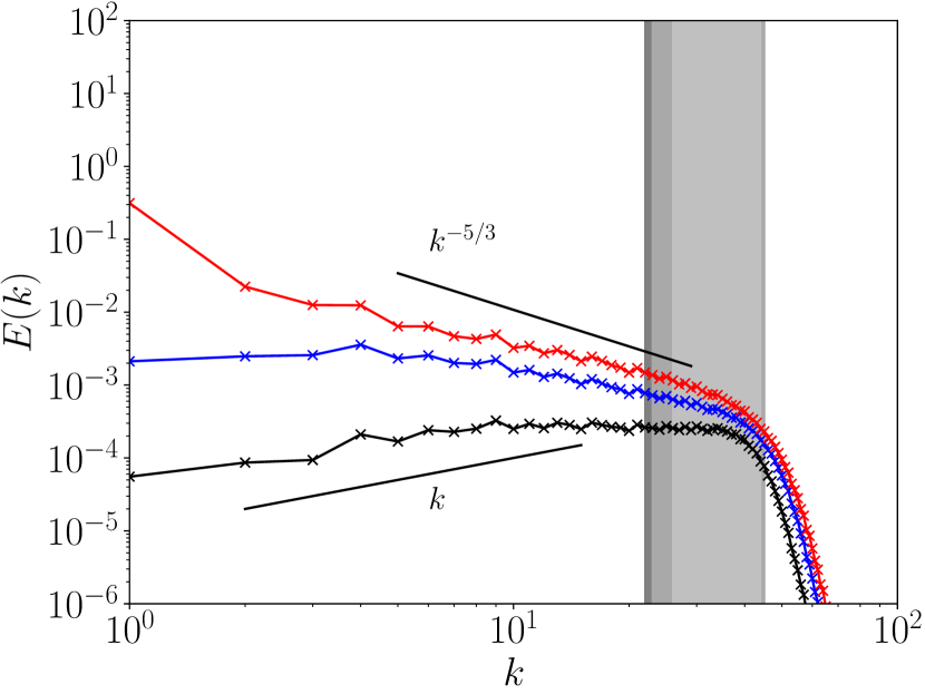
Figure 7: (Color online) Energy spectra. Top: PCV with for different values of $\nu_{1}/\nu_{0}$. The solid lines show the rescaled PCV-B cases $\nu_{1}/\nu_{0}=1$ (black) , $\nu_{1}/\nu_{0}=2$ (blue) and $\nu_{1}/\nu_{0}=5$ (red), and the dotted lines PCV-A data. Bottom: PEV with $\Gamma_{2}/\Gamma_{0}=0.0025$ (red), $\Gamma_{2}/\Gamma_{0}=0.0023$ (blue) and $\Gamma_{2}/\Gamma_{0}=0.002$ (black). The grey-shaded areas indicate the respective driving ranges.

Energy spectra for PCV and PEV are shown in the top and bottom panels of Fig. 7, respectively. The dotted lines in the top panel correspond to series PCV-A, and the solid lines to rescaled PCV-B data as in Ref Linkmann et al. (2019). The transition can be located clearly in the spectra as $E_{1}$ increases by three orders of magnitude from the third to the fourth dotted line. The PEV energy spectra in the bottom panel of Fig. 7 correspond to $\Gamma_{2}/\Gamma_{0}=0.0025$ (red), $\Gamma_{2}/\Gamma_{0}=0.0023$ (blue) and $\Gamma_{2}/\Gamma_{0}=0.002$ (black), with the forcing centered around $k_{\rm f}=36$ as in the PCV model. The results are similar to those for the PCV model shown in the top panel of Fig. 7: A condensate forms suddenly under small changes in the amplification. This further corroborates that the existence and the nature of the transition do not depend on the simplifications of the PEV model that led to the construction of the PCV model. Energy spectra with an extended scaling range and a small accumulation of energy at the smallest wave number have also been observed in the bacterial flow model Oza et al. (2016). There, the critical amplification rate at which the condensate occurs will depend on the relaxation term $-\alpha_{F}{\bm{p}}$ that originates from the functional derivative of the free energy given in Eq. (3). Indeed, the existence of a critical value of $\alpha_{F}>0$, below which no energy accumulation occurs, has been reported in Ref. Bratanov et al. (2015). Similarly, condensate formation in Newtonian turbulence can be suppressed in presence of sufficiently strong linear friction Danilov and Gurarie (2001). In view of the transition scenarios, a general quantification of the effect of large-scale dissipation would be of interest.

At low amplification, equipartition scaling $E(k)\propto k$ is observed for PEV and PCV, as indicated by the black curves in Fig. 7. In contrast, the low-wavenumber form of $E(k)$ is non-universal for the bacterial flow model even at very low amplification Bratanov et al. (2015). This difference also originates from the presence of the relaxation term $-\alpha_{F}{\bm{p}}$ in the bacterial flow model, in Ref. Bratanov et al. (2015) the scaling exponent of $E(k)$ at $k<k_{\rm min}$ is found to depend on $\alpha_{F}$. In Newtonian turbulence, deviations from Kolmogorov-scaling of $E(k)$ also depend on details of large-scale dissipation such as the strength of a linear friction term or the use of hypoviscosity Danilov and Gurarie (2001).

Further observations can be made from the data shown in Fig. 7. The spectral exponent is larger than the Kolmogorov value of $-5/3$ even in presence of an inverse energy transfer, resulting in shallower spectra. This can have several reasons. For simulations with a small condensate such as for the PEV dataset with $\Gamma_{2}/\Gamma_{0}=0.0025$ shown in red (light gray) in the bottom panel, energy dissipation is not negligible in the wavenumber range between the condensate and the driven interval, and Kolmogorov’s hypotheses do not apply. For simulations with a sizeable condensate such as PCV-B3 shown in red (light gray) in the top panel, the condensate itself alters the dynamics in the inertial range. In presence of a strong condensate the spectral scaling is known to become steeper Chertkov et al. (2007), with $E(k)\propto k^{-3}$ for the entire wavenumber range $k<k_{\rm min}$. Removing the coherent part of the velocity field results in shallower scaling $E(k)\propto k^{-1}$ Chertkov et al. (2007). Intermediate states with spectra similar to PCV-B3 have also been obtained, see Fig. 3A in Ref. Chertkov et al. (2007).

V.2 Nonlocal transfers

Since the driving in both models depends on the amount of energy in the driven range, a reduction in the energy input with increasing amplification requires a reduction in $E_{\rm IN}$. One way by which this could happen is through an enhanced nonlinear transfer out of the driven wave number range. The reduction in $E_{\rm IN}$ occurs at the critical point, which suggests that the condensate may couple directly to the driven scales, leading to a non-local spectral energy transfer from the driven wave number interval into the condensate. In order to investigate whether this is the case, the energy transfer spectrum was decomposed into shell-to-shell transfers Domaradzki and Rogallo (1990); Bratanov et al. (2015) between linearly spaced spherical shells centered at wavenumbers $k$ and $q$

$$T(k,q)=\int d\hat{\bm{k}}\int d\hat{\bm{q}}\int d\bm{p}\ \hat{\bm{u}}_{\bm{k}}^{*}\cdot(\hat{\bm{u}}_{\bm{p}}\cdot i\bm{q})\hat{\bm{u}}_{\bm{q}}\delta(\bm{k}+\bm{p}-\bm{q})\ ,$$ (39)

where $\hat{\bm{k}}$ and $\hat{\bm{q}}$ are unit vectors. Here, the focus is on the existence of a coupling between the condensate and the driven scales, hence linear shell-spacing is sufficient. More quantitative statements concerning the relative weight of different couplings within the overall transfer requires logarithmic spacing Aluie and Eyink (2009). Figure 8 shows the non-dimensional transfer $T(k,q)/(\varepsilon_{\rm IN}L_{\rm f}^{2})$ for two example cases, one without condensate (left panel) and one with condensate (right panel). In both cases the transfers are antisymmetric about the diagonal. This must be the case, as energy conservation requires $T(k,q)$ to be antisymmetric under the exchange of $k$ and $q$. As can be seen in the left panel of Fig. 8, in absence of a condensate $T(k,q)$ is concentrated along the diagonal, that is energy is mainly redistributed locally and close to the driven scales. In contrast, the transfers shown in the bottom panel of Fig. 8 include off-diagonal contributions where the condensate couples directly to the driven wavenumber range.

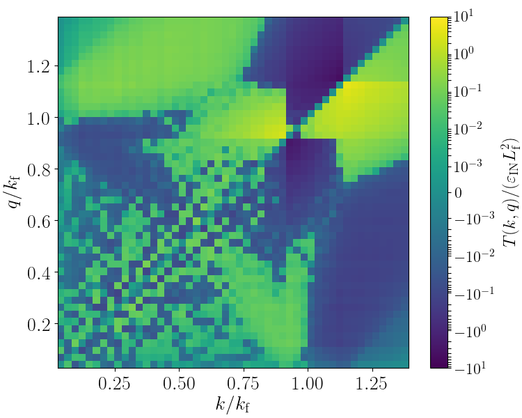
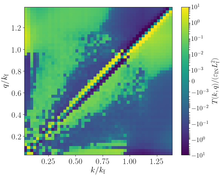
Figure 8: (Color online) PCV shell-to-shell transfer function $T(k,q)/(\varepsilon_{\rm IN}L_{\rm f}^{2})$ for $1\leqslant k,q\leqslant 50$. Left: $\nu_{1}/\nu_{0}=2$, without condensate. Right: $\nu_{1}/\nu_{0}=5$, with condensate at $k=1$.

VI Four-scale model

Some of the qualitative features of the transition can be captured in a four-scale model. Let $E_{\rm LS}$ be the energy content at the intermediate wavenumbers $1<k<k_{\rm min})$ and $E_{\rm SS}$ the energy content at $k>k_{\rm max}$. Then one can consider the interaction of the four quantities $E_{1},E_{\rm IN},E_{\rm LS}$ and $E_{\rm SS}$

$$\dot{E}_{1}= -2\nu_{0}k_{1}^{2}E_{1}+c_{3}E_{1}^{1/2}E_{\rm LS}$$

$$+c_{2}\theta(E_{1}-E_{1,0})(E_{1}-E_{1,0})^{1/2}E_{\rm IN}\ ,$$ (40)

$$\dot{E}_{\rm LS}= -2\nu_{0}k_{\rm LS}^{2}E_{\rm LS}+c_{1}E_{\rm LS}^{1/2}E_{\rm IN}-c_{3}E_{1}^{1/2}E_{\rm LS}\ ,$$ (41)

$$\dot{E}_{\rm IN}= 2\nu_{1}k_{\rm IN}^{2}E_{\rm IN}-c_{1}E_{\rm LS}^{1/2}E_{\rm IN}-c_{4}E_{\rm SS}^{1/2}E_{\rm IN}$$

$$-c_{2}\theta(E_{1}-E_{1,0})(E_{1}-E_{1,0})^{1/2}E_{\rm IN}\ ,$$ (42)

$$\dot{E}_{\rm SS}= -2\nu_{2}k_{\rm SS}^{2}E_{\rm SS}+c_{4}E_{\rm SS}^{1/2}E_{\rm IN}\ ,$$ (43)

where $\theta$ is the Heaviside step function, $c_{i}>0$ for $i=1,\ldots,4$ parametrise the coupling terms and $k_{1}=1$, $k_{\rm LS}$, $k_{\rm IN}$ and $k_{\rm SS}$ are effective wavenumbers in the corresponding ranges. In terms of energy transfers, the coupling terms represent

$$E_{\rm IN}\longrightarrow E_{\rm LS}:\quad c_{1}E_{\rm LS}^{1/2}E_{\rm IN}\ ,$$ (44)

$$E_{\rm IN}\longrightarrow E_{1}:\quad c_{2}\theta(E_{1}-E_{1,0})(E_{1}-E_{1,0})^{1/2}E_{\rm IN}\ ,$$ (45)

$$E_{\rm LS}\longrightarrow E_{1}:\quad c_{3}E_{1}^{1/2}E_{\rm LS}\ ,$$ (46)

$$E_{\rm IN}\longrightarrow E_{\rm SS}:\quad c_{4}E_{\rm SS}^{1/2}E_{\rm IN}\ ,$$ (47)

where the coupling between $E_{\rm IN}$ and $E_{1}$ is modelled such that a nonlocal energy transfer from the driven wavenumber range into the largest resolved scales only takes place once a condensate is emerging. The coupling parameters $c_{i}$ can be obtained from DNS data through calculations of shell-to-shell nonlinear transfers. Once they are known, a parameter scan in $\nu_{1}$ can be carried out for different values of the threshold energy $E_{1,0}$ in order to compare the results from the model with the DNS data. However, before doing so, we derive predictions from the model equations for two asymptotic cases:

• presence of a strong condensate, $E_{1}\gg E_{1,0}$, corresponding to the upper branch in Fig. 6,

• absence of a condensate $E_{1}<E_{1,0}$, corresponding to the lower branch in Fig. 6.

In what follows the small-scale dissipation is neglected, as this enables us to focus on the main points. We will come back to an analysis of the full model in Sec. VI.1.

VI.0.1 case (i): $E_{1}\gg E_{1,0}$

For $E_{1}\gg E_{1,0}$ we approximate the coupling term between $E_{\rm IN}$ and $E_{1}$ as

$$c_{2}\theta(E_{1}-E_{1,0})(E_{1}-E_{1,0})^{1/2}E_{\rm IN}\simeq c_{2}E_{1}^{1/2}E_{\rm IN}\ ,$$ (48)

and we neglect the coupling term $c_{3}E_{1}^{1/2}E_{\rm LS}$ that describes a local energy transfer from the intermediate scales into the condensate. The latter is introduced to model the nonlocal contribution to the inverse energy transfer in presence of a condensate as discussed in Sec. V.2. Equations (VI)-(VI) then simplify to

$$\dot{E}_{\rm IN} =2\nu_{1}k_{\rm IN}^{2}E_{\rm IN}-c_{1}E_{\rm LS}^{1/2}E_{\rm IN}-c_{2}E_{1}^{1/2}E_{\rm IN}\ ,$$ (49)

$$\dot{E}_{\rm LS} =-2\nu_{0}k_{\rm LS}^{2}E_{\rm LS}+c_{1}E_{\rm LS}^{1/2}E_{\rm IN}\ ,$$ (50)

$$\dot{E}_{1} =-2\nu_{0}k_{1}^{2}E_{1}+c_{2}E_{1}^{1/2}E_{\rm IN}\ ,$$ (51)

which result in the following expressions for $E_{\rm IN}$, $E_{\rm LS}$ and $E_{1}$ in steady state

$$2\nu_{1}k_{\rm IN}^{2}E_{\rm IN} =c_{1}E_{\rm LS}^{1/2}E_{\rm IN}+c_{2}E_{1}^{1/2}E_{\rm IN}$$

$$\implies c_{1}E_{\rm LS}^{1/2}+c_{2}E_{1}^{1/2}=-2\nu_{1}k_{\rm IN}^{2}\ ,$$ (52)

$$2\nu_{0}k_{\rm LS}^{2}E_{\rm LS} =c_{1}E_{\rm LS}^{1/2}E_{\rm IN}$$

$$\implies E_{\rm LS}=\left(\frac{c_{1}}{2\nu_{0}k_{\rm LS}^{2}}E_{\rm IN}\right)^{2}\ ,$$ (53)

$$2\nu_{0}k_{1}^{2}E_{1} =c_{2}E_{1}^{1/2}E_{\rm IN}$$

$$\implies E_{1}=\left(\frac{c_{2}}{2\nu_{0}k_{1}^{2}}E_{\rm IN}\right)^{2}\ .$$ (54)

Solving for $E_{\rm IN}$ as a function of $\nu_{1}$, one obtains

$$2\nu_{1}k_{\rm IN}^{2} =c_{1}E_{\rm LS}^{1/2}+c_{2}E_{1}^{1/2}=\frac{\frac{c_{1}^{2}}{2k_{\rm LS}^{2}}+\frac{c_{2}^{2}}{2k_{1}^{2}}}{\nu_{0}}E_{\rm IN}$$

$$\implies E_{\rm IN}=-4\frac{\nu_{1}\nu_{0}k_{\rm IN}^{2}}{\frac{c_{1}^{2}}{k_{\rm LS}^{2}}+\frac{c_{2}^{2}}{k_{1}^{2}}}\ ,$$ (55)

that is, $E_{\rm IN}\sim\nu_{1}$ and $E_{1}\sim\nu_{1}^{2}$, in qualitative agreement with the data presented in Fig. 3 of Ref. Linkmann et al. (2019) for $\nu_{1}>\nu_{1,\rm crit}$, respectively.

VI.0.2 case (ii): $E_{1}<E_{1,0}$

In this case, there is no nonlocal coupling between $E_{1}$ and $E_{\rm IN}$, hence Eqs. (VI)-(VI) become

$$\dot{E}_{\rm IN} =2\nu_{1}k_{\rm IN}^{2}E_{\rm IN}-c_{1}E_{\rm LS}^{1/2}E_{\rm IN}\ ,$$ (56)

$$\dot{E}_{\rm LS} =-2\nu_{0}k_{\rm LS}^{2}E_{\rm LS}+c_{1}E_{\rm LS}^{1/2}E_{\rm IN}-c_{3}E_{1}^{1/2}E_{\rm LS}\ ,$$ (57)

$$\dot{E}_{1} =-2\nu_{0}k_{1}^{2}E_{1}+c_{3}E_{1}^{1/2}E_{\rm LS}\ ,$$ (58)

which leads the the following expressions in steady state

$$2\nu_{1}k_{\rm IN}^{2}E_{\rm IN} =c_{1}E_{\rm LS}^{1/2}E_{\rm IN}$$

$$\implies E_{\rm LS}=\left(\frac{2\nu_{1}k_{\rm IN}^{2}}{c_{1}}\right)^{2}\ ,$$ (59)

$$2\nu_{0}k_{\rm LS}^{2}E_{\rm LS} =c_{1}E_{\rm LS}^{1/2}E_{\rm IN}-c_{3}E_{1}^{1/2}E_{\rm LS}$$

$$\implies E_{\rm IN}=\frac{1}{c_{1}}\left(2\nu_{0}k_{\rm LS}^{2}+c_{3}E_{1}^{1/2}\right)E_{\rm LS}^{1/2}\ ,$$ (60)

$$2\nu_{0}k_{1}^{2}E_{1} =c_{3}E_{1}^{1/2}E_{\rm LS}$$

$$\implies E_{1}=\left(\frac{c_{3}}{2\nu_{0}k_{1}^{2}}E_{\rm LS}\right)^{2}\ .$$ (61)

Solving for $E_{\rm IN}$ as a function of $\nu_{1}$, one obtains

$$E_{\rm IN}=4\frac{\nu_{1}\nu_{0}}{c_{1}^{2}}k_{\rm IN}^{2}\left(k_{\rm LS}^{2}+\left(\frac{c_{3}\nu_{1}k_{\rm IN}^{2}}{c_{1}\nu_{0}k_{1}}\right)^{2}\right)\ ,$$ (62)

while $E_{1}\sim\nu_{1}^{4}$.

Comparing the energy content in the driven wavenumber range between cases (i) and (ii) given in Eqs. (VI.0.1) and (62), respectively, we find

$$E_{\rm IN}^{\varepsilon_{+}} =4\frac{\nu_{1}\nu_{0}k_{\rm IN}^{2}}{\frac{c_{1}^{2}}{k_{\rm LS}^{2}}+\frac{c_{2}^{2}}{k_{1}^{2}}}$$

$$<4\frac{\nu_{1}\nu_{0}}{c_{1}^{2}}k_{\rm IN}^{2}\left(k_{\rm LS}^{2}+\left(\frac{c_{3}\nu_{1}k_{\rm IN}^{2}}{c_{1}\nu_{0}k_{1}}\right)^{2}\right)=E_{\rm IN}^{\varepsilon_{-}}\ .$$ (63)

We point out that this comparison is only justified close to the critical point, as in principle the different cases imply different ranges of $\nu_{1}$: case (i) is applicable for $\nu_{1}>\nu_{1,\rm crit}$ and case (ii) for $\nu_{1}<\nu_{1,\rm crit}$. However, in the vicinity of $\nu_{1,\rm crit}$, Eq. (VI.0.2) predicts a sudden drop in $E_{\rm IN}$ and therefore of $\varepsilon_{\rm IN}=2\nu_{1}k_{\rm IN}^{2}E_{\rm IN}$ as a function of $\nu_{1}$, which is indeed observed in the DNS data as shown in the bottom panel of Fig. 6. In summary, the asymptotics of the model predicts qualitative features of the transition which are in agreement with the DNS results. For further quantitative results, we evaluate the model numerically.

VI.1 Parameter scan for $\nu_{1}$

The results of the previous sections demonstrate that the four-scale model is able to qualitatively reproduce the features of flow states above and below the critical value of $\nu_{1}$. In order to obtain the properties of the transition to a condensate in the model system, we now proceed with a parameter scan. The full model given by eqs. (VI)-(43) is integrated numerically for each value of $\nu_{1}$. The values of the coefficients $c_{i}$, for $1\leqslant i\leqslant 4$ have been chosen based on the values of shell-to-shell transfers Domaradzki and Rogallo (1990); Bratanov et al. (2015) from DNS data above and below the critical point,

$$c_{1} =\frac{T(k=k_{\rm LS},p=k_{\rm IN},q\simeq k_{\rm I})}{\sqrt{E_{\rm LS}}E_{\rm IN}}=0.037\ ,$$ (64)

$$c_{2} =\frac{T(k=k_{1},p=k_{\rm IN},q\simeq k_{\rm IN})}{\sqrt{E_{1}}E_{\rm IN}}=0.043\ ,$$ (65)

$$c_{3} =\frac{T(k=k_{1},p=k_{\rm LS},q\simeq k_{\rm LS})}{\sqrt{E_{1}}E_{\rm LS}}=0.0031\ ,$$ (66)

$$c_{4} =\frac{T(k=k_{\rm SS},p=k_{\rm IN},q\simeq k_{\rm I})}{\sqrt{E_{\rm SS}}E_{\rm IN}}=0.84\ ,$$ (67)

where $k_{1}=1$, $k_{\rm LS}=5$, $k_{\rm IN}=12$ and $k_{\rm SS}=20$. We choose a cutoff value $E_{1,0}=0.05$, which results in a transition in the interval $0<\nu_{1}<1$.

A sharp transition must occur in the four-scale model as the dynamics change at the threshold value $E_{1,0}$ whose qualitative features are remarkably similar to the transition in the full system. Figure 9 presents the results of the parameter scan for $E_{1}$ (left panels) and $\varepsilon_{\rm IN}$ (right panels) as functions of $\nu_{1}$ (top row) and $E_{\rm IN}$ (bottom row). As in the full system, $E_{1}$ shows a sudden jump at a critical value of $\nu_{1}$ and thereafter increases quadratically in $\nu_{1}$, while $E_{\rm IN}$ drops suddenly as predicted for the asymptotic cases in Secs. VI.0.1 and VI.0.2.

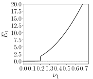
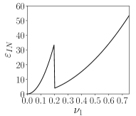
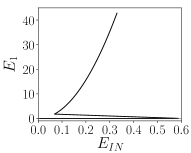
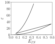
Figure 9: $E_{1}$ (left) and $\varepsilon_{\rm IN}$ (right) as functions of $\nu_{1}$ (top row) and $E_{\rm IN}$ (bottom row) calculated from a parameter scan of eqs. (VI)-(43) and for $E_{1,0}=0.05$.

Furthermore, different states of the model system may be realized at the same value of $\nu_{1}$, as can be seen from the bottom row of Fig. 9, where $E_{1}$ and $\varepsilon$ are presented as functions of $E_{\rm IN}$. The sharp transition is present in form of a discontinuity in the data along a critical line, and for both $E_{1}$ and $\varepsilon$ we observe S-shaped curves with upper and lower branches and an unstable region in between. This is qualitatively similar to the behavior of the full system, as can be seen by comparison with the top panel of Fig. 6, which presents the corresponding DNS data for $E_{1}(\nu_{1}/\nu_{0})$ and with Fig. 3 of Ref. Linkmann et al. (2019) that presents $\varepsilon(\nu_{1}/\nu_{0})$. We point out that the model system is not able to track the second, continuous, transition from absolute equilibrium to viscously damped nonlinear transfers described in Ref. Linkmann et al. (2019), which occurs in the full system at the continuous inflection point of the lower branch $\varepsilon^{-}$. Such an inflection point is not present in the corresponding model data presented in the lower right panel of Fig. 9. This is not surprising as the four-scale model is by construction not able to produce equipartition of energy between all degrees of freedom at $k<k_{\rm min}$.

In summary, the model system adequately reproduces the qualitative features of the transition. The transition is present in the model by construction, where the model dynamics become nonlocal if a threshold energy at the largest scale is reached. As such, we suggest that the transition in the full system also happens through a similar nonlocal coupling scenario: Energy increases at the largest scales through the classical inverse energy cascade and once a threshold energy is crossed, the emerging condensate couples directly to the energy injection range.

VII Conclusions

Active suspensions can be described by a class of one-fluid models that resemble the Navier-Stokes equation supplemented by active driving provided by small-scale instabilities originating from active stresses exerted on the fluid by the microswimmers. Here, we provided a justification of the one-fluid approach for the two-dimensional case by relating the solvent’s velocity field non-locally to the coarse grained polarization field of the active constituents. The resulting model is very similar in structure to solvent models postulated on phenomenological grounds Słomka and Dunkel (2015, 2017a). The justification relies on two main assumptions: The system must be two-dimensional at least to a good approximation and the bacterial concentration must remain constant. That is, it is applicable to dense suspensions in thin layers.

Numerical simulations of a variant of these models showed that a sharp transition occurs between the formation of a steady-state condensate at the largest length scale in the system and a steady-state inverse transfer which is damped by viscous dissipation before reaching the condensate Linkmann et al. (2019). The in-depth investigation carried out here supplements the results of Ref. Linkmann et al. (2019), the system is bistable and shows hysteresis. That is, 2d active matter turbulence and 2d hydrodynamic turbulence with a condensate are two non-equilibrium steady states that can coexist in certain parameter ranges and that are connected through a subcritical transition.

The condensate was found to couple directly to the velocity field fluctuations at the driven scales. This observation led to the introduction of a low-dimensional model that includes such a direct nonlinear coupling once a threshold energy at the largest scales is reached. Analytical and numerical evaluations of the model resulted in a good qualitative agreement with DNS results concerning the main features of the transition. As such, we suggest that the nature of the transition is related to correlations between small- and large-scale velocity fluctuations.

Concerning the nature of the transition, we point out that in systems where the energy input depends on the amount of energy at the driving scales, a reduction in input occurs at the critical point. The latter would not be the case for Gaussian-distributed and $\delta$-in-time correlated random forces as the time-averaged energy input is known a priori. In that case, preliminary results suggest the occurrence of a supercritical transition (work in progress). This suggests that the transition to developed 2d-turbulence is highly non-universal: Depending on the type of forcing there may be no transition, or it may be sub- or supercritical. Similar situations occur in rotating flows Alexakis (2015); Yokoyama and Takaoka (2017); Seshasayanan and Alexakis (2018).

Several aspects of our results merit further investigation. First and foremost, it would be of interest to study transitional behavior experimentally. The Reynolds number necessary for the transition that we found here is at least an order of magnitude larger than those desccribing mesoscale vortices in dense bacterial suspensions. Hence a further increase of swimming speed, a decrease in viscosity or a larger driving scale are required to trigger the transition. All three possibilities present considerable difficulty. The most promising approach may be through the use of non-organic microswimmers. Second, the effect of friction with a substrate, which is present not only in experiments of active suspensions but also in the Newtonian case, on the location of the critical point needs to be quantified.