Simultaneous Inference for Pairwise Graphical Models with Generalized Score Matching

Abstract

Probabilistic graphical models provide a flexible yet parsimonious framework for modeling dependencies among nodes in networks. There is a vast literature on parameter estimation and consistent model selection for graphical models. However, in many of the applications, scientists are also interested in quantifying the uncertainty associated with the estimated parameters and selected models, which current literature has not addressed thoroughly. In this paper, we propose a novel estimator for statistical inference on edge parameters in pairwise graphical models based on generalized Hyvärinen scoring rule. Hyvärinen scoring rule is especially useful in cases where the normalizing constant cannot be obtained efficiently in a closed form, which is a common problem for graphical models, including Ising models and truncated Gaussian graphical models. Our estimator allows us to perform statistical inference for general graphical models whereas the existing works mostly focus on statistical inference for Gaussian graphical models where finding normalizing constant is computationally tractable. Under mild conditions that are typically assumed in the literature for consistent estimation, we prove that our proposed estimator is $\sqrt{n}$-consistent and asymptotically normal, which allows us to construct confidence intervals and build hypothesis tests for edge parameters. Moreover, we show how our proposed method can be applied to test hypotheses that involve a large number of model parameters simultaneously. We illustrate validity of our estimator through extensive simulation studies on a diverse collection of data-generating processes.

Keywords: generalized score matching, high-dimensional inference, probabilistic graphical models, simultaneous inference

1 Introduction

Undirected probabilistic graphical models are widely used to explore and represent dependencies between random variables (Lauritzen, 1996). They have been used in areas ranging from computational biology to neuroscience and finance. An undirected probabilistic graphical model consists of an undirected graph $G=(V,E)$, where $V=\{1,\ldots,p\}$ is the vertex set and $E\subset V\times V$ is the edge set, and a random vector $X=(X_{1},\ldots,X_{p})\in\mathcal{X}^{p}\subseteq\mathbb{R}^{P}$. Each coordinate of the random vector $X$ is associated with a vertex in $V$ and the graph structure encodes the conditional independence assumptions underlying the distribution of $X$. In particular, $X_{a}$ and $X_{b}$ are conditionally independent given all the other variables if and only if $(a,b)\not\in E$, that is, the nodes $a$ and $b$ are not adjacent in $G$. One of the fundamental problems in statistics is that of learning the structure of $G$ from i.i.d. samples from $X$ and quantifying the uncertainty of the estimated structure. Drton and Maathuis (2017) provides a recent review of algorithms for learning the structure, while Janková and van de Geer (2019) provides an overview of statistical inference in Gaussian graphical models.

Gaussian graphical models are a special case of undirected probabilistic graphical models and have been widely studied in the machine learning literature. Suppose that $X\sim\mathcal{N}(\mu,\Sigma)$. In this case, the conditional independence graph is determined by the pattern of non-zero elements of the inverse of the covariance matrix $\Omega=\Sigma^{-1}=(\omega_{ab})$. In particular, $X_{a}$ and $X_{b}$ are conditionally independent given all the other variables in $X$ if and only if $\omega_{ab}$ and $\omega_{ba}$ are both zero. This simple relationship has been fundamental for the development of rich literature on Gaussian graphical models and has facilitated the development of fast algorithms and inferential procedures (see, for example, Dempster, 1972; Drton and Perlman, 2004; Meinshausen and Bühlmann, 2006; Yuan and Lin, 2007; Friedman et al., 2008; Rothman et al., 2008; Yuan, 2010; Sun and Zhang, 2013; Cai et al., 2011).

In this paper, we consider a more general, but still tractable, class of pairwise interaction graphical models with densities belonging to an exponential family $\mathcal{P}=\{p_{\theta}(x)\mid\theta\in\Theta\}$ with natural parameter space $\Theta$:

$$\log p_{\theta}(x)=\sum_{a\in V}\sum_{k\in[K]}\theta_{a}^{(k)}t_{a}^{(k)}(x_{a})\\ +\sum_{(a,b)\in E}\sum_{l\in[L]}\theta_{ab}^{(l)}t_{ab}^{(l)}(x_{a},x_{b})-\Psi(\theta)+\sum_{a\in V}h_{a}(x_{a}),\quad x\in\mathcal{X}\subseteq\mathbb{R}^{p}.$$ (1)

The functions $t_{a}^{(k)}$, $t_{ab}^{(l)}$ are the sufficient statistics and $\Psi(\theta)$ is the log-partition function. We assume throughout the paper that the support of the densities is either $\mathcal{X}=\mathbb{R}^{p}$ or $\mathcal{X}=\mathbb{R}^{p}_{+}$ and $\mathcal{P}$ is dominated by Lebesgue measure on $\mathbb{R}^{p}$. To simplify the notation, for a log-density of the form given in (1) we will write

$$\log p_{\theta}(x)=\theta^{\top}t(x)-\Psi(\theta)+h(x),$$

where $\theta\in\mathbb{R}^{s}$ and $t(x):\mathbb{R}^{p}\mapsto\mathbb{R}^{s}$ with $s=L\cdot{p\choose 2}+p\cdot K$. The natural parameter space has the form $\Theta=\{\theta\in\mathbb{R}^{s}\mid\Psi(x)=\log\int_{\mathcal{X}}\exp(\theta^{\top}t(x)dx)<\infty\}$. Under the model in (1), there is no edge between $a$ and $b$ in the corresponding conditional independence graph if and only if $\theta_{ab}^{(1)}=\cdots=\theta_{ab}^{(L)}=0$. The model in (1) encompasses a large number of graphical models studied in the literature as we discuss in Section 1.2. Lin et al. (2016) studied estimation of parameters in model (1), however, the focus of this paper, as we discuss next, is on performing statistical inference—constructing honest confidence intervals and statistical tests—for parameters in (1).

The focus of the paper is on the inferential analysis about parameters in the model given in (1), as well as the Markov dependencies between observed variables. Our inference procedure does not rely on the oracle support recovery properties of the estimator and is therefore uniformly valid in a high-dimensional regime and robust to model selection mistakes, which commonly occur in ultra-high dimensional setting. Our approach is based on Hyvärinen generalized scoring rule estimate of $\theta$ in (1). The same procedure was used in Lin et al. (2016), however, rather than focusing on consistent model selection, we use the initial estimator to construct a regular linear estimator (van der Vaart, 1998). We establish Bahadur type representation for our final regular estimator that is robust to model selection mistakes and valid for a big class of data generating distributions. The purpose of establishing a Bahadur representation is to approximate an estimate by a sum of independent random variables, and hence prove the asymptotic normality of the estimator for (1), allowing us to conduct statistical inference on the model parameters (see Bahadur, 1966). In particular, we show how to construct confidence intervals for a parameter in the model that have nominal coverage and also propose a statistical test for existence of edges in the graphical model with nominal size. These results complement existing literature, which is focused on consistent model selection and parameter recovery, as we review in the next section. Furthermore, we develop a methodology for constructing simultaneous confidence intervals for all the parameters in the model (1) and apply this methodology for testing the parameters in the differential network. The main idea here is to use the Gaussian multiplier bootstrap to approximate the distribution of the maximum coordinate of the linear part in the Bahadur representation. Appropriate quantile obtained from the bootstrap distribution is used to approximate the width of the simultaneous confidence intervals and the cutoff values for the tests for the parameters of the differential network.

1.1 Main Contribution

This paper makes two major contributions to the literature on statistical inference for graphical models. First, compared to previous work on high-dimensional inference in graphical models (Ren et al., 2015; Barber and Kolar, 2018; Wang and Kolar, 2016; Janková and van de Geer, 2015), this is the first work on statistical inference in models where computing the log-partition function is intractable. Existing works mostly focus on Gaussian graphical models with a tractable normalizing constant, whereas our method can be applied to more general models, as we discuss in Section 2.1. Second, we apply our proposed method to simultaneous inference on all edges connected to a specific node. Our simultaneous inference procedure can be used to

1. test whether a node is isolated in a graph; that is, whether it is conditionally independent with all the other nodes;

2. estimate the support of the graph by setting an appropriate threshold on the proposed estimators; and

3. test for the difference between graphical models where we have observations of two graphical models with the same nodes and we would like to test whether the local connectivity pattern for a specific node is the same in the two graphs.

Once again, the existing approaches cannot deal with simultaneous testing with an intractable normalizing constant. Moreover, most of the existing work impose a sparsity condition on the inverse of Hessian and focus on $L=1$ only. Here we relax the sparsity condition on the inverse Hessian and show how to perform inference for a general $L$.

1.2 Related Work

Our work straddles two areas of statistical learning which have attracted significant research of late: model selection and estimation in high-dimensional graphical models, and high-dimensional inference. We briefly review the literature most relevant to our work, and refer the reader to two recent review articles for a comprehensive overview (Drton and Maathuis, 2017; Janková and van de Geer, 2019). Drton and Maathuis (2017) focuses on structure learning in graphical models, while Janková and van de Geer (2019) reviews inference in Gaussian graphical models.

We start by reviewing the literature on learning structure of probabilistic graphical models. Much of the research effort has focused on learning structure of Gaussian graphical models where the edge set $E$ of the graph $G$ is encoded by the non-zero elements of the precision matrix $\Omega=\Sigma^{-1}$. The literature here roughly splits into two categories: global and local methods. Global methods typically estimate the precision matrix by maximizing regularized Gaussian log-likelihood (Yuan and Lin, 2007; Rothman et al., 2008; Friedman et al., 2008; d’Aspremont et al., 2008; Ravikumar et al., 2011; Fan et al., 2009; Lam and Fan, 2009), while local methods estimate the graph structure by learning the neighborhood or Markov blanket of each node separately (Meinshausen and Bühlmann, 2006; Yuan, 2010; Cai et al., 2011; Liu and Wang, 2017; Zhao and Liu, 2014). Extensions to more general distributions in Gaussian and elliptical families are possible using copulas, as the graph structure within these families is again determined by the inverse of the latent correlation matrix (Liu et al., 2009, 2012a; Xue and Zou, 2012; Liu et al., 2012b; Fan et al., 2017).

Once we depart from the Gaussian distribution and related families, learning the conditional independence structure becomes more difficult, primarily owing to computational intractability of evaluating the log-partition function. A computationally tractable alternative to regularized maximum likelihood estimation is regularized pseudo-likelihood which was studied in the context of learning structure of Ising models in Höfling and Tibshirani (2009), Ravikumar et al. (2010), and Xue et al. (2012). Similar methods were developed in the study of mixed exponential family graphical models, where a node’s conditional distribution is a member of an exponential family distribution, such as Bernoulli, Gaussian, Poisson or exponential. See Guo et al. (2011a), Guo et al. (2011b), Lee and Hastie (2015), Cheng et al. (2013), Yang et al. (2012), and Yang et al. (2014) for more details.

More recently, score matching estimators have been investigated for learning the structure of graphical models in high-dimensions when the normalizing constant is not available in a closed-form (Lin et al., 2016; Yu et al., 2018). Score matching was first proposed in Hyvärinen (2005) and subsequently extended for binary models and models with non-negative data in Hyvärinen (2007). It offers a computational advantage when the normalization constant is not available in a closed-form, making likelihood based approaches intractable, and is particularly appealing for estimation in exponential families as the objective function is quadratic in the parameters of interest. Sun et al. (2015) develop a method based on score matching for learning conditional independence graphs underlying structured infinite-dimensional exponential families. Forbes and Lauritzen (2015) investigated the use of score matching for the inference of Gaussian linear models in low-dimensional settings. However, despite its power, there have not been results on inference in high-dimensional models using score matching. As one of our contributions in this paper, we build on the prior work on estimation using generalized score matching and develop an approach to statistical inference for high-dimensional graphical models. In particular, we construct a novel $\sqrt{n}$-consistent estimator of parameters in (1). This is the first procedure that can obtain a parametric $\sqrt{n}$ rate of convergence for an edge parameter in a graphical model where computing the normalizing constant is intractable.

Next, we review the literature on high-dimensional inference, focusing on work related to high-dimensional undirected graphical models. Liu (2013) developed a procedure that estimates conditional independence graph from Gaussian observations and controls false discovery rates asymptotically. Wasserman et al. (2014) develop confidence guarantees for undirected graphs under minimal assumptions by developing Berry-Esseen bounds on the accuracy of Normal approximation. Ren et al. (2015), Janková and van de Geer (2015), and Janková and van de Geer (2017) develop methods for constructing confidence intervals for edge parameters in Gaussian graphical models, based on the idea of debiasing the $\ell_{1}$ regularized estimator developed in (Zhang and Zhang, 2013; van de Geer et al., 2014; Javanmard and Montanari, 2014). A related approach was developed for edge parameters in mixed graphical models whose node conditional distributions belong to an exponential family in Wang and Kolar (2016). Wang and Kolar (2014) develop methodology for performing statistical inference in time-varying and conditional Gaussian graphical models, while Barber and Kolar (2018) and Lu et al. (2018) develop methods for semi-parametric copula models. We contribute to the literature on high dimensional inference by demonstrating how to construct regular estimators for probabilistic Graphical models whose normalizing constant is intractable. Our estimators are robust to model selection mistakes and allows us to perform valid statistical inference for edge parameters in a large family of data generating distributions.

Finally, we contribute to the literature on simultaneous inference in high-dimensional models. Zhang and Cheng (2017) and Dezeure et al. (2017) develop methods for performing simultaneous inference on all the coefficients in a high-dimensional linear regression. In the same setting, Zhao et al. (2014) use a multiplier bootstrap approach to construct robust simultaneous confidence intervals. Chang et al. (2018) applies it to the simultaneous inference of Gaussian graphical models. These procedures allow for the dimensionality of the vector to be exponential in the sample size and rely on bootstrap to approximate the quantile of the test statistic. We extend these ideas to the high dimensional graphical model setting and show how we can build simultaneous hypothesis tests on the neighbors of a specific node.

A conference version of this paper was presented in the Annual Conference on Neural Information Processing Systems 2016 (Yu et al., 2016). Compared to the conference version, in this paper we extend the results in the following ways. First, we extend the results to include the generalized score matching method (Yu et al., 2018, 2019) in place of the original score matching method. This generalized form of the score matching method allows us to improve the estimation accuracy and obtain better inference results for non-negative data. In the conference version, we made an assumption that the inverse of the population Hessian matrix, see Section 4, is (approximately) sparse. We relax this sparsity condition and develop an inference procedure that is valid even if the sparsity condition is violated, but the inverse of the Hessian matrix has bounded columns in the $\ell_{1}$ norm. Moreover, instead of focusing on a single edge as in the conference version, in this work we propose a procedure for simultaneous inference for all edges connected to a specific node. This allows us to build hypothesis tests for a broad class of applications, including testing of isolated nodes, support recovery, and testing the difference between two graphical models. Furthermore, while the conference version focused on the case where $L=1$ in (1), here we extend the results to a general choice of $L$. Lastly, we run additional experiments to demonstrate the effectiveness of our proposed method.

1.3 Notation

We use $[n]$ to denote the set $\{1,\ldots,n\}$. For a vector $a\in\mathbb{R}^{n}$, we let ${\rm supp}(a)=\{j\ :\ a_{j}\neq 0\}$ be the support set (with an analogous definition for matrices $A\in\mathbb{R}^{n_{1}\times n_{2}}$), $\|a\|_{q}$, $q\in[1,\infty)$, the $\ell_{q}$-norm defined as $\|a\|_{q}=(\sum_{i\in[n]}|a_{i}|^{q})^{1/q}$ with the usual extensions for $q\in\{0,\infty\}$, that is, $\|a\|_{0}=|{\rm supp}(a)|$ and $\|a\|_{\infty}=\max_{i\in[n]}|a_{i}|$. For a vector $x$, $x_{M}$ is a sub-vector of $x$ with components corresponding to the set $M$, and $x_{-ab}$ is the sub-vector with component corresponding to edge $\{a,b\}$ omitted. For a matrix $A\in\mathbb{R}^{m\times n}$, denote $\|A\|_{q}=\sup\{\|Ax\|_{q}:x\in\mathbb{R}^{n},\|x\|_{q}=1\}$ as the induced $\ell_{q}$ norm. In particular, $\|A\|_{\infty}=\max_{1\leq i\leq m}\sum_{j=1}^{n}|a_{ij}|$. We also use $\|A\|_{\max}=\max_{jk}|a_{jk}|$ to denote the maximum component of $A$. We define $\mathbb{E}_{n}$ as the empirical mean of $n$ samples: $\mathbb{E}_{n}[f(x_{i},\theta)]=\frac{1}{n}\sum_{i=1}^{n}f(x_{i},\theta)$. For two sequences of numbers $\{a_{n}\}_{n=1}^{\infty}$ and $\{b_{n}\}_{n=1}^{\infty}$, we use $a_{n}=\mathcal{O}(b_{n})$, or $a_{n}\lesssim b_{n}$ to denote that $a_{n}\leq Cb_{n}$ for some finite positive constant $C$, and for all $n$ large enough. We use $a_{n}\lesssim_{P}b_{n}$ to denote that $a_{n}\lesssim b_{n}$ happens with high probability. The notation $a_{n}=o(b_{n})$ is used to denote that $a_{n}b_{n}^{-1}\xrightarrow{n\rightarrow\infty}0$. We denote $a_{n}\longrightarrow_{D}\mathcal{A}$ as convergence in distribution to a fixed distribution $\mathcal{A}$ and $a_{n}\longrightarrow_{P}a$ as convergence in probability to a constant $a$. We denote $a\circ b=(a_{1}b_{1},...,a_{p}b_{p})$ for $a,b\in\mathbb{R}^{p}$. For any function $f:\mathbb{R}^{p}\to\mathbb{R}$, we use $\nabla f(x)=\left\{\partial/(\partial x_{j})f(x)\right\}_{j\in[p]}$ to denote the gradient, and $\Delta f(x)=\sum_{j\in[p]}\partial^{2}/(\partial x_{j}^{2})f(x)$ to denote the Laplacian operator on $\mathbb{R}^{p}$. Note that both the gradient and the Laplacian are with respect to $x$.

1.4 Organization of the Paper

The remainder of this paper is structured as follows. We begin in Section 2 with background on exponential family pairwise graphical model, score matching method, and a brief review of statistical inference in high dimensional models. In Section 3 we describe the construction of our novel estimator for a single edge parameter based on a three-step procedure, for $L=1$. Section 4 provides theoretical results and Section 5 discusses the relaxation of sparsity condition on the inverse of population Hessian matrix. Section 6 extends the procedure to simultaneous inference for all edges connected to some specific node. In Section 7 we extend our results to general $L$. We provide experimental results for synthetic datasets and a real dataset in Sections 8 and 9 respectively. Section 10 provides conclusion and discussion.

2 Background

We begin with reviewing exponential family pairwise graphical models in Section 2.1, and then introduce the score matching and generalized score matching methods in Section 2.2. Finally we provide a brief overview of statistical inference for high dimensional models in Section 2.3.

2.1 Exponential Family Pairwise Graphical Models

Throughout the paper we focus on the case where

$$\mathcal{P}=\{p_{\theta}(x)\mid\theta\in\Theta\}$$

is an exponential family with log-densities given in (1), which frequently appear in graphical modeling. There are $K$ sets of sufficient statistics $\{t_{a}^{(k)}\}_{k\in[K]}$ for each $a\in V$ that depend on the individual nodes and $L$ sets of sufficient statistics for each $(a,b)\in{V\choose 2}$ that allow for pairwise interactions of different types. Conditional independence graph underlying a distribution $p_{\theta}\in\mathcal{P}$ has no edge between vertices $a$ and $b$ if and only if $\theta_{ab}^{(1)}=\ldots=\theta_{ab}^{(L)}=0$. A special case of the model given in (1) are pairwise interaction models with log-densities

$$\log p_{\theta}(x)=\sum_{(a,b)\in E}\theta_{ab}t_{ab}(x_{a},x_{b})-\Psi(\theta)+h(x),\quad x\in\mathcal{X}\subseteq\mathbb{R}^{p},$$ (2)

where $t_{ab}(x_{a},x_{b})$ are sufficient statistics that depend only on $x_{a}$ and $x_{b}$. In what follows, we will consider models that either has the form given in (2) or the more general form given in (1).

A number of well-studied distributions have the above discussed form. We provide some examples below, including examples where the normalizing constant $\Psi(\theta)$ cannot be obtained in closed-form.

Gaussian graphical models.

The most studied example of a probabilistic graphical model is the case of the Gaussian graphical model. Suppose that the random variable $X$ follows the centered multivariate Gaussian distribution with covariance $\Sigma$ and precision matrix $\Omega=\Sigma^{-1}=(\omega_{ab})$. The log-density is given as

$$p(x;\Omega)\propto\exp\left\{-\frac{1}{2}x^{\top}\Omega x\right\},$$ (3)

the support of the density is $\mathcal{X}=\mathbb{R}^{p}$ and the sufficient statistics take the form $t_{ab}(x_{a},x_{b})=x_{a}x_{b}$.

Non-negative Gaussian.

Our second example of a distribution with the log-density of the form in (2) is that of a non-negative Gaussian random vector. The probability density function of a non-negative Gaussian random vector $X$ is proportional to that of the corresponding Gaussian vector given in (3), but restricted to the non-negative orthant. Here the support of the density is $\mathcal{X}=\mathbb{R}_{+}^{p}$. The conditional independence graph is determined the same way as in the Gaussian graphical model case through the non-zero pattern of the elements in the precision matrix $\Omega$. The normalizing constant in this family has no closed-form and hence maximum likelihood estimation of $\Omega$ is intractable.

Normal conditionals.

Our third example is taken from Lin et al. (2016). See also Gelman and Meng (1991) and Arnold et al. (1999). Consider the family of distributions with densities of the form

$$p(x;\Theta^{(1)},\Theta^{(2)},\eta,\beta)\propto\exp\left\{\sum_{a\neq b}\Theta_{ab}^{(2)}x_{a}^{2}x_{b}^{2}+\sum_{a\neq b}\Theta_{ab}^{(1)}x_{a}x_{b}+\sum_{a\in V}\eta_{a}x_{a}^{2}+\sum_{a\in V}\beta_{a}x_{a}\right\},\,x\in\mathbb{R}^{p},$$

where the matrices $\Theta^{(1)},\Theta^{(2)}\in\mathbb{R}^{p\times p}$ are symmetric interaction matrices with a zero diagonal. Members of this family have Normal conditionals, but the densities themselves need not be unimodal. The conditional independence graph does not contain an edge between vertices $a$ and $b$ if and only if both $\Omega_{ab}^{(1)}$ and $\Omega_{ab}^{(2)}$ are equal to zero. In contrast to the Gaussian graphical models, the conditional dependence may also express itself in the variances.

Conditionally specified mixed graphical models.

In general, specifying multivariate distributions is difficult, since in a given problem it might not be clear what class of graphical models to use. On the other hand, specifying univariate distributions is an easier task. Chen et al. (2015) and Yang et al. (2015) explored ways of specifying multivariate joint distributions via univariate exponential families. Consider a conditional density of the form

$$p(x_{a}\mid(x_{b},b\neq a);\theta_{a})=\exp\left\{f_{a}(x_{a})+\sum_{b\neq a}\theta_{ab}B_{a}(x_{a})B_{b}(x_{b})-\Psi_{a}(\eta_{a})\right\},\quad x_{a}\in\mathcal{X}_{a},$$ (4)

where $\eta_{a}=\eta_{a}(\theta_{a},f_{a},(x_{b})_{b\neq a})$ and $B_{a}(\cdot)$ are known functions for each $a\in V$. Suppose that for a random vector $X$, each coordinate $X_{a}$ follows the conditional density of the form in (4) with $\theta_{ab}=\theta_{ba}$ for all $a,b\in V$. Then Chen et al. (2015) and Yang et al. (2015) showed that there exists a joint distribution of $X$ compatible with the conditional densities and that it is of the form

$$p(x;\Theta)\propto\exp\left\{\sum_{a\in V}f_{a}(x_{a})+\frac{1}{2}\sum_{a\in V}\sum_{b\neq a}\theta_{ab}B_{a}(x_{a})B_{b}(x_{b})\right\},\quad x\in\mathcal{X}.$$

In particular, the joint density above is of the form given in (1), with pairwise interaction sufficient statistics given as $t_{ab}(x_{a},x_{b})=B_{a}(x_{a})B_{b}(x_{b})$. When the support of the distribution is $\mathcal{X}=\mathbb{R}^{p}$ or $\mathcal{X}=\mathbb{R}_{+}^{p}$, the parameters of the distribution can be efficiently estimated using score matching. In the case of unknown function $B_{a}(\cdot)$, Suggala et al. (2017) explored nonparametric estimation via basis expansion and fitted parameters using pseudo-likelihood. Developing a valid statistical inference procedure for this nonparametric setting is beyond the scope of the current work.

As an example of a conditionally specified model, that we will return to later in the paper, consider exponential graphical models where the node-conditional distributions follow an exponential distribution. For a random vector $X$ described by an exponential graphical model, the density function is given by

$$p(x;\Theta)\propto\exp\left\{-\sum_{a\in V}\theta_{a}x_{a}-\sum_{a\neq b}\theta_{ab}x_{a}x_{b}\right\},\quad x\in\mathbb{R}^{p}_{+}.$$

Note that the variable takes only non-negative values. To ensure that the distribution is valid and normalizable, the natural parameter space $\Theta$ consists of matrices whose elements are positive. Therefore, one can only model negative dependencies via the exponential graphical model.

Exponential square-root graphical model.

As our last example, consider the exponential square-root graphical model (Inouye et al., 2016) with density function given by

$$p(x;\eta,K)\propto\exp\left\{-\sqrt{x}^{\top}K\sqrt{x}+2\eta^{\top}\sqrt{x}\right\},\quad x\in\mathbb{R}^{p}_{+}.$$

This square-root graphical model is a multivariate generalizations of univariate exponential family distributions that can capture the positive dependency among nodes. Specifically, it assumes only a mild condition on the parameter matrix, but allows for almost arbitrary negative and positive dependencies. We refer to Inouye et al. (2016) for details on parameter estimation with nodewise regressions and likelihood approximation methods.

2.2 Score Matching

In this section we briefly review the score matching method proposed in Hyvärinen (2005, 2007) and the generalized score matching for non-negative data proposed in Yu et al. (2018).

2.2.1 Score Matching

A scoring rule $S(x,Q)$ is a real-valued function that quantifies the accuracy of $Q\in\mathcal{P}$ being the distribution from which an observed realization $x\in\mathcal{X}$ may have been sampled. There are a large number of scoring rules that correspond to different decision problems Parry et al. (2012). Given $n$ independent realizations of $X$, $\{x_{i}\}_{i\in[n]}$, one finds optimal score estimator $\widehat{Q}\in\mathcal{P}$ that minimizes the empirical score

$$\widehat{Q}=\arg\min_{Q\in\mathcal{P}}\mathbb{E}_{n}\left[S(x_{i},Q)\right].$$ (5)

When $\mathcal{X}=\mathbb{R}^{p}$ and $\mathcal{P}$ consists of twice differentiable densities with respect to Lebesgue measure, the Hyvärinen scoring rule (Hyvärinen, 2005) is given as

$$S(x,Q)=\frac{1}{2}\big{\|}\nabla\log q(x)\big{\|}_{2}^{2}+\Delta\log q(x),$$ (6)

where $q$ is the density of $Q$ with respect to Lebesgue measure on $\mathcal{X}$. We would like to emphasize that this gradient and Laplacian are with respect to $x$. In this way we get rid of the normalizing constant which does not depend on $x$. This scoring rule is convenient for learning models that are specified in an unnormalized fashion or whose normalizing constant is difficult to compute. The score matching rule is proper (Dawid, 2007), that is, $\mathbb{E}_{X\sim P}S(X,Q)$ is minimized over $\mathcal{P}$ at $Q=P$. Suppose the density $q$ of $Q\in\mathcal{P}$ is twice continuously differentiable and satisfies

$$\mathbb{E}_{X\sim P}\|\nabla\log q(X)\|_{2}^{2}<\infty,\qquad\text{for all $P,Q\in\mathcal{P}$}$$

and

$$q(x)\text{ and }\|\nabla q(x)\|_{2}\text{ tend to zero as $x$ approaches the boundary of $\mathcal{X}$ }.$$

Then the Fisher divergence between $P,Q\in\mathcal{P}$,

$$D(P,Q)=\int p(x)\|\nabla\log q(x)-\nabla\log p(x)\|_{2}^{2}dx,$$

where $p$ is the density of $P$, is induced by the score matching rule (Hyvärinen, 2005). The gradients in the equation above can be thought of as gradients with respect to a hypothetical location parameter, evaluated at the origin (Hyvärinen, 2005).

For a parametric exponential family $\mathcal{P}=\{p_{\theta}\mid\theta\in\Theta\}$ with densities given in (1), minimizing (5) with the scoring rule in (6) can be done in a closed form (Hyvärinen, 2005; Forbes and Lauritzen, 2015). An estimator $\widehat{\theta}$ obtained in this way can be shown to be asymptotically consistent (Hyvärinen, 2005), however, in general it will not be efficient (Forbes and Lauritzen, 2015).

2.2.2 Generalized Score Matching for Non-Negative Data

The score matching method in Section 2.2.1 does not work for non-negative data, since the assumption that $q(x)$ and $||\nabla q(x)||_{2}$ tend to 0 at the boundary breaks down. To solve this problem, Hyvärinen (2007) proposed a generalization of the score matching approach to the case of non-negative data.

When $\mathcal{X}=\mathbb{R}^{p}_{+}$ the non-negative score matching loss (analogous to the Fisher divergence $D(P,Q)$) is defined as

$$J_{+}(P,Q)=\int_{\mathbb{R}^{p}_{+}}p(x)\cdot\big{\|}\nabla\log p(x)\circ x-\nabla\log q(x)\circ x\big{\|}_{2}^{2}dx.$$

The scoring rule for non-negative data that induces $J_{+}(P,Q)$ is given as

$$S_{+}(x,Q)={\sum_{a\in V}\left[2x_{a}\frac{\partial\log q(x)}{\partial x_{a}}+x_{a}^{2}\frac{\partial^{2}\log q(x)}{\partial x_{a}^{2}}+\frac{1}{2}x_{a}^{2}\left(\frac{\partial\log q(x)}{\partial x_{a}}\right)^{2}\right]}.$$ (7)

For exponential families, the non-negative score matching loss again can be obtained in a closed form and the estimator is consistent and asymptotically normal under suitable conditions (Hyvärinen, 2007).

Yu et al. (2018) proposed the generalized score matching for non-negative data to improve the estimation efficiency of the procedure based on the scoring rule in (7). Let $\ell_{1},...,\ell_{p}:\mathbb{R}_{+}\to\mathbb{R}_{+}$ be positive and differentiable functions and set

$$\ell(x)=\big{(}\ell_{1}(x_{1}),\ldots,\ell_{p}(x_{p})\big{)}.$$

The generalized $\ell$-score matching loss is defined as

$$J_{\ell}(P,Q)=\int_{\mathbb{R}^{p}_{+}}p(x)\cdot\big{\|}\nabla\log p(x)\circ\ell^{1/2}(x)-\nabla\log q(x)\circ\ell^{1/2}(x)\big{\|}_{2}^{2}dx,$$

where $\ell^{1/2}(x)=\big{(}\ell_{1}^{1/2}(x_{1}),\ldots,\ell_{p}^{1/2}(x_{p})\big{)}$. Suppose the following regularity conditions are satisfied

$$\lim_{x_{j}\to\infty}p(x)\ell_{j}(x_{j})\nabla_{j}\log q(x)=0~{}~{}~{}~{}\forall x_{-j}\in\mathbb{R}^{p-1}_{+},~{}\forall p\in\mathcal{P}_{+},$$ (8)

$$\lim_{x_{j}\to 0}p(x)\ell_{j}(x_{j})\nabla_{j}\log q(x)=0~{}~{}~{}~{}\forall x_{-j}\in\mathbb{R}^{p-1}_{+},~{}\forall p\in\mathcal{P}_{+},$$

$$\mathbb{E}_{X\sim\mathcal{P}_{+}}\Big{[}\|\nabla\log q(X)\circ\ell^{1/2}(X)\|_{2}^{2}\Big{]}<+\infty,$$

$$\mathbb{E}_{X\sim\mathcal{P}_{+}}\Big{[}\|(\nabla\log q(X)\circ\ell(X))^{\prime}\|_{1}\Big{]}<+\infty.$$

Under the condition (8), the scoring rule corresponding to the generalized $\ell$-score matching loss is given as

$$S_{\ell}(x,Q)={\sum_{a\in V}\left[\ell^{\prime}_{a}(x_{a})\frac{\partial\log q(x)}{\partial x_{a}}+\ell_{a}(x_{a})\frac{\partial^{2}\log q(x)}{\partial x_{a}^{2}}+\frac{1}{2}\ell_{a}(x_{a})\left(\frac{\partial\log q(x)}{\partial x_{a}}\right)^{2}\right]}.$$

The regularity condition (8) is required for applying integration by parts and Fubini-Tonelli theorem in order to show consistency of the score-matching estimator.

Note that by choosing $\ell_{j}(x)=x^{2}$, for all $j$, one recovers the original score matching formulas for non-negative data in (7). The advantage of this generalized score matching rule is that by choosing an increasing, but slowly growing $\ell(x)$ (for example, $\ell(x)=\log(x+1)$), one does not need to estimate high moments of the underlying distribution, which leads to better practical performance and improved theoretical guarantees. See Yu et al. (2018) for details.

2.2.3 Score matching for probabilistic graphical models

Score matching has been successfully applied in the context of probabilistic graphical models. Forbes and Lauritzen (2015) studied score matching to learn Gaussian graphical models with symmetry constraints. Lin et al. (2016) proposed a regularized score matching procedure to learn conditional independence graph in a high-dimensional setting by minimizing

$$\mathbb{E}_{n}\left[\overline{S}(x_{i},\theta)\right]+\lambda\|\theta\|_{1},$$

where the loss function $\overline{S}(x_{i},\theta)$ is either $S(x_{i},Q_{\theta})$ defined in (6) or $S_{+}(x_{i},Q_{\theta})$ defined in (7). For Gaussian models, $\ell_{1}$-norm regularized score matching is a simple, yet efficient method, which coincides with the method in Liu and Luo (2015). Yu et al. (2018) improved on the approach of Lin et al. (2016) and studied regularized generalized $\ell$-score matching of the form

$$\mathbb{E}_{n}\left[S_{\ell}(x_{i},Q_{\theta})\right]+\lambda\|\theta\|_{1}.$$

Applied to data generated from a multivariate truncated normal distribution, the conditional independence graph can be recovered with the same number of samples that are needed for recovery of the structure of a Gaussian graphical model. Sun et al. (2015) develop a score matching estimator for learning the structure of nonparametric probabilistic graphical models, extending the work on estimation of infinite-dimensional exponential families (Sriperumbudur et al., 2017). In Section 3, we present a new estimator for components of $\theta$ in (1) that is consistent and asymptotically normal, building on Lin et al. (2016) and Yu et al. (2018).

2.3 Statistical Inference

We briefly review how to perform statistical inference for low dimensional parameters in a high-dimensional model. In many statistical problems, the unknown parameter $\beta\in\mathbb{R}^{p}$ can be partitioned as $\beta=(\alpha,\eta)$, where $\alpha$ is a scalar of interest and $\eta$ is a $(p-1)$ dimensional nuisance parameter. Let $\beta^{*}=(\alpha^{*},\eta^{*})$ denote the true unknown parameter. In a high-dimensional setting, where the sample size $n$ is much smaller than the dimensionality $p$ of the parameter $\beta$, it is common to impose structural assumptions on $\beta^{*}$. For example in several applications, it is common to assume that the true parameter $\beta^{*}$ is sparse. Indeed, we will work under this assumption as well.

Let us denote the empirical negative log-likelihood by

$$\mathcal{L}(\beta)=\frac{1}{n}\sum_{i=1}^{n}\mathcal{L}_{i}(\beta),$$

where $\mathcal{L}_{i}(\beta)$ is the negative log-likelihood for the $i^{th}$ observation. Let $I=\mathbb{E}\left[\nabla^{2}\mathcal{L}(\beta)\right]$ denote the information matrix and denote the partition of $I$ corresponding to $\beta=(\alpha,\eta)$ as

$$I=\begin{pmatrix}I_{\alpha\alpha}&I_{\alpha\eta}\\ I_{\eta\alpha}&I_{\eta\eta}\end{pmatrix}.$$ (9)

The partial information matrix of $\alpha$ is denoted as $I_{\alpha|\eta}=I_{\alpha\alpha}-I_{\alpha\eta}I_{\eta\eta}^{-1}I_{\eta\alpha}$.

Consider for the moment a low-dimensional setting. In order to perform statistical inference about $\alpha^{*}$, one can use the profile partial score function defined as

$$U(\alpha)=\nabla_{\alpha}\mathcal{L}\big{(}\alpha,\widehat{\eta}(\alpha)\big{)},$$

where $\widehat{\eta}(\alpha)=\arg\min_{\eta}\mathcal{L}(\alpha,\eta)$ is the maximum partial likelihood estimator for $\eta$ with a fixed parameter $\alpha$. Under the null hypothesis that $\alpha^{*}=\alpha^{0}$, we have that (van der Vaart, 1998)

$$\sqrt{n}U\left(\alpha^{0}\right)\longrightarrow_{D}N(0,I_{\alpha|\eta}^{*}).$$

Therefore, one can reject the null hypothesis for large values of $U\left(\alpha^{0}\right)$. However, in a high-dimensional setting, the estimator $\widehat{\eta}(\alpha)$ is no longer $\sqrt{n}$-consistent and we have to modify the approach above. In particular, we will show how to modify the profile partial score function to allow for valid inference in a high-dimensional setting based on a sparse estimator of $\widehat{\eta}(\alpha)$.

Without loss of generality, assume that $\alpha^{0}=0$. For any estimator $\widetilde{\eta}$, Taylor’s expansion theorem gives

$$\sqrt{n}\nabla_{\alpha}\mathcal{L}(0,\widetilde{\eta})=\sqrt{n}\nabla_{\alpha}\mathcal{L}(0,\eta^{*})+\sqrt{n}\nabla_{\alpha\eta}\mathcal{L}(0,\eta^{*})\cdot(\widetilde{\eta}-\eta^{*})+\textsf{rem},$$ (10)

where rem is the remainder $o(\widetilde{\eta}-\eta^{*})$ term. The first term $\sqrt{n}\nabla_{\alpha}\mathcal{L}(0,\eta^{*})$ in (10) converges to a normal distribution under suitable assumptions using the central limit theorem (CLT). The distribution of the second term, however, is in general intractable to obtain. This is due to the fact that the distribution of $\widetilde{\eta}$ depends on the selected model. Unless we are willing to assume stringent and untestable conditions under which it is possible to show that the true model can be selected, the limiting distribution of $\widetilde{\eta}$ cannot be estimated even asymptotically (Leeb and Pötscher, 2007). To overcome this issue, one needs to modify the profile partial score function, so that its limiting distribution does not depend on the way the nuisance parameter is estimated.

Ning and Liu (2017) introduced the following decorrelated score function

$$U(\alpha,\eta)=\nabla_{\alpha}\mathcal{L}(\alpha,\eta)-w^{T}\nabla_{\eta}\mathcal{L}(\alpha,\eta),$$

where $w=I_{\alpha\eta}I_{\eta\eta}^{-1}$. The decorrelated score function $U(\alpha,\eta)$ is uncorrelated with the nuisance score functions $\nabla_{\eta}\mathcal{L}(\alpha,\eta)$ and, therefore, its limiting distribution will not depend on the model selection mistakes incurred while estimating $\eta^{*}$. In particular, $U(\alpha^{0},\widetilde{\eta})$ is indeed asymptotically normally distributed under the null hypothesis, as long as $\widetilde{\eta}$ is a good enough estimator of $\eta^{*}$, but not necessarily $\sqrt{n}$-consistent estimator. Based on the asymptotic normality of the decorrelated score function, we can then build confidence intervals for $\alpha^{*}$ and perform hypothesis testing.

In practice, the vector $w$ is unknown and needs to be estimated. A number of methods have been proposed for its estimation in the literature. For example, Ning and Liu (2017) use a Dantzig selector-like method, Belloni et al. (2013) proposed the double selection method, while Zhang and Zhang (2013), van de Geer et al. (2014), and Javanmard and Montanari (2014) use a lasso based estimator. See also Dezeure et al. (2017), Zhang and Cheng (2017) for simultaneous inference, Taylor et al. (2014), Yang et al. (2016) for post selective inference, Li (2019), Cao and Dowd (2019), and Cao and Lu (2019) for for synthetic control, etc. In this paper, we adopt the double selection procedure of Belloni et al. (2013). Details will be given in Section 3.

3 Methodology

In this section, we present a new procedure that constructs a $\sqrt{n}$-consistent estimator of an element $\theta_{ab}$ of $\theta$. Our procedure involves three steps that we detail below. We start by introducing some additional notation and then describe the procedure for the case where $\mathcal{X}=\mathbb{R}^{p}$. Extension to non-negative data is given at the end of the section. Throughout this section we consider $L=1$ only, so that the parameter of interest $\theta_{ab}$ is a scalar. Extensions to general $L$ is discussed later in Section 7.

For fixed indices $a,b\in[p]$, let

$$q^{ab}_{\theta}(x):=q^{ab}_{\theta}(x_{a},x_{b}\mid x_{-ab})$$

be the conditional density of $(X_{a},X_{b})$ given $X_{-ab}=x_{-ab}$. In particular,

$$\log q^{ab}_{\theta}(x)=\langle{\theta^{ab}},{\varphi(x)}\rangle-\Psi^{ab}(\theta,x_{-ab})+h^{ab}(x),$$ (11)

where $\theta^{ab}\in\mathbb{R}^{s^{\prime}}$, with $s^{\prime}=2K+2p-3$, is the part of the vector $\theta$ corresponding to $\left\{\theta_{a}^{(k)},\theta_{b}^{(k)}\right\}_{k\in[K]}$, $\left\{\theta_{ac},\theta_{bc}\right\}_{c\in-ab}$, and $\theta_{ab}$; and $\varphi(x)=\varphi^{ab}(x)\in\mathbb{R}^{s^{\prime}}$ is the corresponding vector of sufficient statistics $\left\{t_{a}^{(k)}(x_{a}),t_{b}^{(k)}(x_{b})\right\}_{k\in[K]}$, $\left\{t_{ac}(x_{a},x_{c}),t_{bc}(x_{b},x_{c})\right\}_{c\in-ab}$, and $t_{ab}(x_{a},x_{b})$. Here $\Psi^{ab}(\theta,x_{-ab})$ is the log-partition function of the conditional distribution and $h^{ab}(x)=h_{a}(x_{a})+h_{b}(x_{b})$. Let $\nabla_{ab}$ and $\Delta_{ab}$ be the gradient and Laplacian operators, respectively, with respect to $x_{a}$ and $x_{b}$ defined as:

$$\nabla_{ab}f(x) =\Big{(}(\partial/\partial x_{a})f(x),(\partial/\partial x_{b})f(x)\Big{)}^{\top}\in\mathbb{R}^{2},$$

$$\Delta_{ab}f(x) =\Big{(}(\partial^{2}/\partial x_{a}^{2})+(\partial^{2}/\partial x_{b}^{2})\Big{)}f(x).$$

With this notation, we introduce the following scoring rule

$$S^{ab}(x,\theta)=\frac{1}{2}\big{\|}\nabla_{ab}\log q^{ab}_{\theta}(x)\big{\|}_{2}^{2}+\Delta_{ab}\log q^{ab}_{\theta}(x)=\frac{1}{2}\theta^{\top}\Gamma(x)\theta+\theta^{\top}g(x)+c(x),$$ (12)

where the constant term $c(x)=\frac{1}{2}\|\nabla h^{ab}(x)\|^{2}+\Delta h^{ab}(x)$, and

$$\Gamma(x)=\varphi_{1}(x)\varphi_{1}(x)^{\top}+\varphi_{2}(x)\varphi_{2}(x)^{\top}\quad\text{ and }\quad g(x)=\varphi_{1}(x)h_{1}^{ab}(x)+\varphi_{2}(x)h_{2}^{ab}(x)+\Delta_{ab}\varphi(x)$$

with $\varphi_{1}=(\partial/\partial x_{a})\varphi$, $\varphi_{2}=(\partial/\partial x_{b})\varphi$, $h_{1}^{ab}=(\partial/\partial x_{a})h^{ab}$, and $h_{2}^{ab}=(\partial/\partial x_{b})h^{ab}$.

This scoring rule is related to the one in (6), however, rather than using the density $q_{\theta}$ in evaluating the parameter vector, we only consider the conditional density $q_{\theta}^{ab}$. We will use this conditional scoring rule to create an asymptotically normal estimator of an element $\theta_{ab}$. Our motivation for using this estimator comes from the fact that the parameter $\theta_{ab}$ can be identified from the conditional distribution of $(X_{a},X_{b})\mid X_{M_{ab}}$ where

$$M_{ab}:=\{c\mid(a,c)\in E\text{ or }(b,c)\in E\}$$

is the Markov blanket of $(X_{a},X_{b})$. Furthermore, the optimization problems arising in steps 1-3 below can be solved much more efficiently, as the scoring rule in (12) involves fewer parameters.

We are now ready to describe our procedure for estimating $\theta_{ab}$, which proceeds in three steps.

Step 1:

We find a pilot estimator of $\theta^{ab}$ by solving the following program

$$\widehat{\theta}^{ab} =\arg\min_{\theta\in\mathbb{R}^{s^{\prime}}}\ \mathbb{E}_{n}\left[S^{ab}(x_{i},\theta)\right]+\lambda_{1}\|\theta\|_{1},$$ (13)

where $\lambda_{1}$ is a tuning parameter. Let $\widehat{M}_{1}={\rm supp}(\widehat{\theta}^{ab}):=\{(c,d)\mid\widehat{\theta}^{ab}_{cd}\neq 0\}$.

Since we are after an asymptotically normal estimator of $\theta_{ab}$, one may think that it is sufficient to find $\widetilde{\theta}^{ab}=\arg\min\{\mathbb{E}_{n}\left[S^{ab}(x_{i},\theta)\right]\mid{\rm supp}(\theta)\subseteq\widehat{M}_{1}\}$ and appeal to results of Portnoy (1988), who has established asymptotic normality for $M$-estimators with increasing number of parameters. Unfortunately, this is not the case. Since $\widetilde{\theta}$ is obtained via a model selection procedure, it is irregular and its asymptotic distribution cannot be estimated (Leeb and Pötscher, 2007; Pötscher, 2009). Therefore, we proceed to create a regular estimator of $\theta_{ab}$ in steps 2 and 3. The idea is to create an estimator $\widetilde{\theta}_{ab}$ that is insensitive to first-order perturbations of other components of $\widetilde{\theta}^{ab}$, which we consider as nuisance components. The idea of creating an estimator that is robust to perturbations of nuisance has been recently used in Belloni et al. (2013), however, the approach goes back to the work of Neyman (1959).

Step 2:

Let $\widehat{\gamma}^{ab}$ be a minimizer of

$$\frac{1}{2}\mathbb{E}_{n}[(\varphi_{1,ab}(x_{i})-\varphi_{1,-ab}(x_{i})^{\top}\gamma)^{2}+(\varphi_{2,ab}(x_{i})-\varphi_{2,-ab}(x_{i})^{\top}\gamma)^{2}]+\lambda_{2}\|\gamma\|_{1},$$ (14)

where $\lambda_{2}$ is a tuning parameter. Let $\widehat{M}_{2}={\rm supp}(\widehat{\gamma}^{ab}):=\{(c,d)\mid\widehat{\gamma}^{ab}_{cd}\neq 0\}$. The intuition here is that the vector $(1,-\widehat{\gamma}^{ab,\top})^{\top}$ approximately computes a row, up to a constant, of the inverse of the Hessian in (13).

Step 3:

Let $\widetilde{M}=\{(a,b)\}\cup\widehat{M}_{1}\cup\widehat{M}_{2}$. We obtain our estimator as a solution to the following program

$$\widetilde{\theta}^{ab} =\arg\min_{\theta}\ \mathbb{E}_{n}\left[S^{ab}(x_{i},\theta)\right]\qquad\text{s.t.}\quad{\rm supp}(\theta)\subseteq\widetilde{M}.$$ (15)

Our estimator of $\theta_{ab}$ is the coordinate $ab$ of $\widetilde{\theta}^{ab}$—which we denote as $\widetilde{\theta}_{ab}$. Motivation for this procedure will be clear from the proof of Theorem 2 given in the next section.

Extension to non-negative data.

For non-negative data, the procedure is similar. In place of the score rule in (12), we will use a conditional score rule based on the generalized $\ell$-score rule. We define the following scoring rule

$$S^{ab}_{\ell}(x,\theta)=\frac{1}{2}\theta^{\top}\Gamma_{\ell}(x)\theta+\theta^{\top}g_{\ell}(x)$$ (16)

with

$$\Gamma_{\ell}(x)=\ell_{a}(x_{a})\cdot\varphi_{1}(x)\varphi_{1}(x)^{\top}+\ell_{b}(x_{b})\cdot\varphi_{2}(x)\varphi_{2}(x)^{\top}$$

and

$$g_{\ell}(x)=\ell_{a}(x_{a})\varphi_{1}(x)h_{1}^{ab}(x)+\ell_{b}(x_{b})\varphi_{2}(x)h_{2}^{ab}(x) +\ell_{a}(x_{a})\varphi_{11}(x)+\ell_{b}(x_{b})\varphi_{22}(x)$$

$$\qquad+\ell^{\prime}_{a}(x_{a})\varphi_{1}(x)+\ell^{\prime}_{b}(x_{b})\varphi_{2}(x).$$

Here $\varphi_{11}=(\partial^{2}/\partial x_{a}^{2})\varphi$, and $\varphi_{22}=(\partial^{2}/\partial x_{b}^{2})\varphi$. Now we can define

$$\widetilde{\varphi}_{1}=\ell^{1/2}_{a}(x_{a})\varphi_{1}\quad\text{and}\quad\widetilde{\varphi}_{2}=\ell^{1/2}_{b}(x_{b})\varphi_{2}.$$ (17)

Then $\Gamma_{\ell}(x)=\widetilde{\varphi}_{1}(x)\widetilde{\varphi}_{1}(x)^{\top}+\widetilde{\varphi}_{2}(x)\widetilde{\varphi}_{2}(x)^{\top}$, which is of the same form as (12) with $\widetilde{\varphi}_{1}$ and $\widetilde{\varphi}_{2}$ replacing $\varphi_{1}$ and $\varphi_{2}$, respectively. Thus our three-step procedure for non-negative data can be written as follows. For notation consistency, we omit the subscript $\ell$ on the estimator $\theta$ and support $M$.

Step 1:

We find a pilot estimator of $\theta^{ab}$ by solving

$$\widehat{\theta}^{ab} =\arg\min_{\theta\in\mathbb{R}^{s^{\prime}}}\ \mathbb{E}_{n}\left[S_{\ell}^{ab}(x_{i},\theta)\right]+\lambda_{1}\|\theta\|_{1},$$ (18)

where $\lambda_{1}$ is a tuning parameter and $S_{\ell}^{ab}$ is defined in (16). Let $\widehat{M}_{1}={\rm supp}(\widehat{\theta}^{ab})$.

Step 2:

Let $\widehat{\gamma}^{ab}$ be a minimizer of

$$\frac{1}{2}\mathbb{E}_{n}\big{[}(\widetilde{\varphi}_{1,ab}(x_{i})-\widetilde{\varphi}_{1,-ab}(x_{i})^{\top}\gamma)^{2}+(\widetilde{\varphi}_{2,ab}(x_{i})-\widetilde{\varphi}_{2,-ab}(x_{i})^{\top}\gamma)^{2}\big{]}+\lambda_{2}\|\gamma\|_{1},$$ (19)

where $\lambda_{2}$ is a tuning parameter and $\widetilde{\varphi}_{1},\widetilde{\varphi}_{2}$ are defined in (17). Let $\widehat{M}_{2}={\rm supp}(\widehat{\gamma}^{ab})$.

Step 3:

Let $\widetilde{M}=\{(a,b)\}\cup\widehat{M}_{1}\cup\widehat{M}_{2}$. We obtain our estimator as a solution to the following program

$$\widetilde{\theta}^{ab} =\arg\min_{\theta}\ \mathbb{E}_{n}\left[S_{\ell}^{ab}(x_{i},\theta)\right]\qquad\text{s.t.}\quad{\rm supp}(\theta)\subseteq\widetilde{M}.$$ (20)

Our estimator of $\theta_{ab}$ is the coordinate $ab$ of $\widetilde{\theta}^{ab}$—which we denote as $\widetilde{\theta}_{ab}$.

4 Asymptotic Normality of the Estimator

In this section, we outline the main theoretical properties of our estimator. We start by providing high-level conditions that allow us to establish properties of each step in the procedure.

Assumption M.

We are given $n$ i.i.d. samples $\{x_{i}\}_{i\in[n]}$ from $p_{\theta^{*}}$ of the form in (1). Let

$$\gamma^{ab,*} =\arg\min_{\gamma}\ \mathbb{E}[(\varphi_{1,ab}(x_{i})-\varphi_{1,-ab}(x_{i})^{\top}\gamma)^{2}+(\varphi_{2,ab}(x_{i})-\varphi_{2,-ab}(x_{i})^{\top}\gamma)^{2}]$$ (21)

and

$$\eta_{1i}=\varphi_{1,ab}(x_{i})-\varphi_{1,-ab}(x_{i})^{\top}\gamma^{ab,*}~{}~{}~{}\text{and}~{}~{}~{}\eta_{2i}=\varphi_{2,ab}(x_{i})-\varphi_{2,-ab}(x_{i})^{\top}\gamma^{ab,*}~{}~{}~{}\text{for}~{}i\in[n].$$

We assume that the parameter vector $\theta^{*}$ is sparse with $|{\rm supp}(\theta^{ab,*})|\ll n$; and the vector $\gamma^{ab,*}$ is sparse with $|{\rm supp}(\gamma^{ab,*})|\ll n$.

Let $m=|{\rm supp}(\theta^{ab,*})|\vee|{\rm supp}(\gamma^{ab,*})|$. The assumption M supposes that the parameter to be estimated is sparse, which makes estimation in the high-dimensional setting feasible. An extension to the approximately sparse parameter is possible but technically cumbersome, and does not provide additional insights into the problem. One of the benefits of using the conditional score to learn parameters of the model is that the sample size will only depend on the size of ${\rm supp}(\theta^{ab,*})$ and not on the sparsity of the whole vector $\theta^{*}$ as in Lin et al. (2016). The second part of the assumption states that the inverse of the population Hessian is approximately sparse, which is a reasonable assumption for a number of models, since the Markov blanket of $(X_{a},X_{b})$ is small under the sparsity assumption on $\theta^{ab,*}$. We relax the sparsity assumption in Section 5.

The vector $\gamma^{ab,*}$ is determined by the model (11) and parameter $\theta^{*}$, and is therefore not a free parameter. For the Gaussian graphical model, it can be shown that the sparsity of $\theta^{ab,*}$ implies the sparsity of $\gamma^{ab,*}$. That is, assumption M holds when the columns of the precision matrix are sparse. For a general model, it may not be easy to explicitly verify the exact sparsity of $\gamma^{ab,*}$, since the calculation of $\gamma^{ab,*}$ involves calculation of possibly intractable moments, especially when using generalized score matching with $\ell(x)=\log(x+1)$ for non-negative data. For normal conditionals and exponential graphical model, we verify numerically (in Section 8) that the sample version of $\gamma^{ab,*}$ behaves approximately like a sparse vector when $n$ is large enough. These indicate that assumption M is reasonable, at least in an approximately sparse version. For general models, the sparsity condition on $\gamma^{ab,*}$ could be violated and, therefore, we discuss how to relax it in Section 5.

Our next condition assumes that the Hessian in (13) and (14) is well conditioned.

Assumption SE.

Let

$$\phi_{-}(s,A)=\inf\left\{\delta^{\top}A\delta/\|\delta\|_{2}^{2}\mid 1\leq\|\delta\|_{0}\leq s\right\}$$

and

$$\phi_{+}(s,A)=\sup\left\{\delta^{\top}A\delta/\|\delta\|_{2}^{2}\mid 1\leq\|\delta\|_{0}\leq s\right\}$$

denote the minimal and maximal $s$-sparse eigenvalues of a semi-definite matrix $A$, respectively. We assume

$$\phi_{\min}\leq\phi_{-}(m\cdot\log n,\mathbb{E}\left[\Gamma(x_{i})\right])\leq\phi_{+}(m\cdot\log n,\mathbb{E}\left[\Gamma(x_{i})\right])\leq\phi_{\max},$$

where $0<\phi_{\min}\leq\phi_{\max}<\infty$.

Assumption SE imposes the sparse eigenvalue condition on the population quantity. A lower bound on the population Hessian is required even in a low dimensional setting in order to prove asymptotic normality of an estimator. See, for example, Forbes and Lauritzen (2015) where the population Hessian is assumed to be invertible. An upper bound on the Hessian matrix is also commonly assumed in the literature on graphical models and high-dimensional inference (see, for example, Yang et al., 2015; Belloni and Chernozhukov, 2013). We use the upper bound on the Hessian to control the size of the estimated support in steps 1 and 2 of the procedure.

For Gaussian graphical model, assumption SE is satisfied with non-degenerate covariance matrix. For general models, assumption SE puts restrictions on the model parameter in a way that is hard to handle explicitly. Note that related work imposes stronger assumption on the sample Fisher information matrix directly. See, for example, conditions (C1) and (C2) in Yang et al. (2015).

For the upper bound of the sparse eigenvalue, we remark that the mean of $\varphi(x)$ could be non-zero. For the Gaussian graphical model, if there is a non-zero mean $\mu$, then the components of $\varphi_{1}(x)$ and $\varphi_{2}(x)$ would instead be $x-\mu$. Therefore the sparse eigenvalue would not explode. In practice, we subtract the empirical mean and only need to consider the centered case. For other models, existing works assume boundedness of the first and second order moments of all the components of $x$. See Condition (C3) in Yang et al. (2015).

With assumption SE on the population quantity, the following lemma, adopted from Corollary 4 in Belloni and Chernozhukov (2013), quantifies the sparse eigenvalues of the sample quantity $\mathbb{E}_{n}\left[\Gamma(x_{i})\right]$.

Lemma 1

Suppose assumption SE is satisfied. Suppose there exist $K_{n}$ such that $\varphi_{1}(x_{i})$ and $\varphi_{2}(x_{i})$ are bounded: $\sup_{i}\|\varphi_{1}(x_{i})\|_{\infty}\leq K_{n}$ and $\sup_{i}\|\varphi_{2}(x_{i})\|_{\infty}\leq K_{n}$ a.s. If the sample size satisfies

$$K_{n}^{2}\cdot m\log{p}\cdot\log^{2}(m\log{p})\cdot\log{n}\cdot\log{(p\vee n)}=o(n\phi_{\min}^{2}/\phi_{\max}),$$

then the event

$$\mathcal{E}_{\rm SE}=\left\{\frac{\phi_{\min}}{2}\leq\phi_{-}\big{(}m\cdot\log n,\mathbb{E}_{n}\left[\Gamma(x_{i})\right]\big{)}\leq\phi_{+}\big{(}m\cdot\log n,\mathbb{E}_{n}\left[\Gamma(x_{i})\right]\big{)}\leq 2\phi_{\max}\right\}$$

holds with probability at least $1-o(1)$.

Lemma 1 ensures that the sparse eigenvalues of the sample quantity $\mathbb{E}_{n}\left[\Gamma(x_{i})\right]$ are well-behaved provided that $\varphi_{1}(x_{i})$ and $\varphi_{2}(x_{i})$ can be upper bounded, and the sample size is reasonably large. The scale of the upper bound $K_{n}$ depends on the sufficient statistics $\varphi(x)$, and can be verified for concrete models. For example, for the Gaussian graphical model, a standard result on the Gaussian tail bound gives $K_{n}=C\cdot(\log n+\log p)^{1/2}$ with high probability. As another example, Proposition 4 in Yang et al. (2015) shows that, under mild conditions, $K_{n}=C\cdot(\log n+\log p)$ with high probability when the sufficient statistics of the conditional density are given by $x_{a},x_{b}$ and $x_{a}x_{b}$, which includes a wide range of applications, such as exponential graphical model, and Poisson graphical model. For models with more general sufficient statistics, we can modify the proof of Proposition 4 in Yang et al. (2015) to obtain the corresponding rate on $K_{n}$, under suitable assumptions.

Let $r_{j\theta}=\|\widehat{\theta}^{ab}-\theta^{ab,*}\|_{j}$ and $r_{j\gamma}=\|\widehat{\gamma}^{ab}-\gamma^{ab,*}\|_{j}$, for $j\in\{1,2\}$, be the rates of estimation in steps 1 and 2, respectively. Under the assumption SE, on the event

$$\mathcal{E}_{\theta}=\left\{\|\mathbb{E}_{n}\left[\Gamma(x_{i})\theta^{ab,*}+g(x_{i})\right]\|_{\infty}\leq\frac{\lambda_{1}}{2}\right\},$$

we have that $r_{1\theta}\lesssim m\lambda_{1}/\phi_{\min}$ and $r_{2\theta}\lesssim c_{2}\sqrt{m}\lambda_{1}/\phi_{\min}$. Similarly, on the event

$$\mathcal{E}_{\gamma}=\left\{\|\mathbb{E}_{n}\left[\eta_{1i}\varphi_{1,-ab}(x_{i})+\eta_{2i}\varphi_{2,-ab}(x_{i})\right]\|_{\infty}\leq\frac{\lambda_{2}}{2}\right\},$$

we have that $r_{1\gamma}\lesssim m\lambda_{2}/\phi_{\min}$ and $r_{2\gamma}\lesssim\sqrt{m}\lambda_{2}/\phi_{\min}$, using results of Negahban et al. (2012). In order to ensure that $\mathcal{E}_{\theta}$ and $\mathcal{E}_{\gamma}$ hold with high-probability, one needs to choose appropriate $\lambda_{1}$ and $\lambda_{2}$. This calculation is specific to the model at hand. For example, if the vectors

$$\Gamma(x_{i})\theta^{ab,*}+g(x_{i})\quad\text{and}\quad\eta_{1i}\varphi_{1,-ab}(x_{i})+\eta_{2i}\varphi_{2,-ab}(x_{i})$$ (22)

have sub-Gaussian components, then by taking $\lambda_{1},\lambda_{2}\propto\sqrt{\log p/n}$, the events $\mathcal{E}_{\theta}$ and $\mathcal{E}_{\gamma}$ hold with probability at least $1-c_{1}p^{-c_{2}}$ (Yang et al., 2015; Negahban et al., 2012). For other distributions, we may need to choose larger $\lambda_{1}$ and $\lambda_{2}$. See also Lemma 9 in Yang et al. (2015).

The following result establishes a Bahadur representation for $\widetilde{\theta}_{ab}$.

Theorem 2

Suppose that assumptions M and SE hold. Define $w^{*}$ with $w^{*}_{ab}=1$ and $w^{*}_{-ab}=-\gamma^{ab,*}$, where $\gamma^{ab,*}$ is given in the assumption M. On the event $\mathcal{E}_{\gamma}\cap\mathcal{E}_{\theta}$, we have that

$$\sqrt{n}\cdot\left(\widetilde{\theta}_{ab}-\theta_{ab}^{*}\right) =-\sigma_{n}^{-1}\cdot\sqrt{n}\mathbb{E}_{n}\left[w^{*\top}\left(\Gamma(x_{i})\theta^{ab,*}+g(x_{i})\right)\right]+\mathcal{O}\left(\phi_{\max}^{2}\phi_{\min}^{-4}\cdot\sqrt{n}\lambda_{1}\lambda_{2}m\right),$$ (23)

where $\sigma_{n}=\mathbb{E}_{n}\left[\eta_{1i}\varphi_{1,ab}(x_{i})+\eta_{2i}\varphi_{2,ab}(x_{i})\right]$.

Theorem 2 is deterministic in nature. It establishes a representation that holds on the event $\mathcal{E}_{\gamma}\cap\mathcal{E}_{\theta}\cap\mathcal{E}_{\rm SE}$, which in many cases holds with overwhelming probability. We will show that under suitable conditions the first term converges to a normal distribution. The following assumption is a regularity condition needed even in a low dimensional setting for asymptotic normality of the score matching estimator (Forbes and Lauritzen, 2015).

Assumption R.

$\mathbb{E}_{q^{ab}}\left[\|\Gamma(X_{a},X_{b},x_{-ab})\theta^{ab,*}\|^{2}\right]$ and $\mathbb{E}_{q^{ab}}\left[\|g(X_{a},X_{b},x_{-ab})\|^{2}\right]$ are finite for all values of $x_{-ab}$ in the domain.

Theorem 2 and Lemma 15 (Appendix A) together give the following corollary:

Corollary 3

Suppose that the conditions of Theorem 2 hold. In addition, suppose the assumption R holds, $\sqrt{n}\lambda_{1}\lambda_{2}m=o(1)$ and $\mathbb{P}\left(\mathcal{E}_{\gamma}\cap\mathcal{E}_{\theta}\cap\mathcal{E}_{\rm SE}\right)\rightarrow 1$. Then we have

$$\sqrt{n}(\widetilde{\theta}_{ab}-\theta_{ab}^{*})\longrightarrow_{D}N(0,V_{ab}),$$

where $V_{ab}=\left(\mathbb{E}\left[\sigma_{n}\right]\right)^{-2}\cdot\operatorname*{{\rm Var}}\left(w^{*\top}\left(\Gamma(x_{i})\theta^{ab,*}+g(x_{i})\right)\right)$ and $\sigma_{n}$ is as in Theorem 2.

When the vectors in (22) are sub-Gaussian, we choose $\lambda_{1},\lambda_{2}\propto\sqrt{\log p/n}$, so that the sample complexity is given by $(m\log{p})^{2}/n=o(1)$. For other distributions, we may need a larger sample size to bound the error term in (23). We see that the variance $V_{ab}$ depends on the true $\theta^{ab,*}$ and $\gamma^{ab,*}$, which are unknown. In practice, we estimate $V_{ab}$ using the following consistent estimator $\widehat{V}_{ab}$,

$$\widehat{V}_{ab}=e_{ab}^{\top}\left(\mathbb{E}_{n}\left[\Gamma(x_{i})\right]_{\widetilde{M}}\right)^{-1}\cdot Z\cdot\left(\mathbb{E}_{n}\left[\Gamma(x_{i})\right]_{\widetilde{M}}\right)^{-1}e_{ab},$$ (24)

with

$$Z={\mathbb{E}_{n}\left[\left(\Gamma(x_{i})\widetilde{\theta}^{ab}+g(x_{i})\right)_{\widetilde{M}}\left(\Gamma(x_{i})\widetilde{\theta}^{ab}+g(x_{i})\right)_{\widetilde{M}}^{\top}\right]},$$

and $e_{ab}$ being a canonical vector with $1$ in the position of element $ab$ and $0$ elsewhere. The consistency of this variance estimator is provided in the appendix. Using this estimate, we can construct a confidence interval with asymptotically nominal coverage. In particular,

$$\lim_{n\rightarrow\infty}\sup_{\theta^{*}\in\Theta}\mathbb{P}_{\theta^{*}}\left(\theta_{ab}^{*}\in\widetilde{\theta}_{ab}\pm z_{\kappa/2}\cdot\sqrt{\widehat{V}_{ab}/n}\right)=\kappa.$$

In the next section, we outline the proof of Theorem 2. Proofs of other technical results are relegated to appendix.

4.1 Proof of Theorem 2

We first introduce some auxiliary estimates. Let $\widetilde{\gamma}^{ab}$ be a minimizer of the following constrained problem

$$\min_{\gamma}\ \,\mathbb{E}_{n}\left[\left(\varphi_{1,ab}(x_{i})-\varphi_{1,-ab}(x_{i})^{\top}\gamma\right)^{2}+\left(\varphi_{2,ab}(x_{i})-\varphi_{2,-ab}(x_{i})^{\top}\gamma\right)^{2}\right]\$$ (25)

$$\text{ s.t. }\ \,{\rm supp}(\gamma)\subseteq\widetilde{M}\backslash(a,b),$$

where $\widetilde{M}$ is defined in the step 3 of the procedure. Essentially, $\widetilde{\gamma}^{ab}$ is the refitted estimator from step 2 constrained to have the support on $\widetilde{M}\backslash(a,b)$. Let $\widetilde{w}\in\mathbb{R}^{s^{\prime}}$ with $\widetilde{w}_{ab}=1$, $\widetilde{w}_{\widetilde{M}\backslash(a,b)}=-\widetilde{\gamma}_{\widetilde{M}\backslash(a,b)}$ and zero elsewhere. The solution $\widetilde{\theta}^{ab}$ satisfies the first order optimality condition $\left(\mathbb{E}_{n}\left[\Gamma(x_{i})\right]\widetilde{\theta}^{ab}+\mathbb{E}_{n}[g(x_{i})]\right)_{\widetilde{M}}=0$. Multiplying by $\widetilde{w}$, it follows that

$$\widetilde{w}^{\top}\left(\mathbb{E}_{n}\left[\Gamma(x_{i})\right]\widetilde{\theta}^{ab}+\mathbb{E}_{n}[g(x_{i})]\right)$$ (26)

$$= \left(\widetilde{w}-w^{*}\right)^{\top}\mathbb{E}_{n}\left[\Gamma(x_{i})\right]\left(\widetilde{\theta}^{ab}-\theta^{ab,*}\right)+\left(\widetilde{w}-w^{*}\right)^{\top}\left(\mathbb{E}_{n}\left[\Gamma(x_{i})\theta^{ab,*}+g(x_{i})\right]\right)$$

$$\qquad+w^{*\top}\mathbb{E}_{n}\left[\Gamma(x_{i})\right]\left(\widetilde{\theta}^{ab}-\theta^{ab,*}\right)+w^{*\top}\left(\mathbb{E}_{n}\left[\Gamma(x_{i})\theta^{ab,*}+g(x_{i})\right]\right)$$

$$\triangleq L_{1}+L_{2}+L_{3}+L_{4}=0.$$

From Lemma 12 and Lemma 13 (Appendix A), we have that

$$\left|L_{1}+L_{2}\right|\lesssim\phi_{\max}^{2}\phi_{\min}^{-4}\cdot\lambda_{1}\lambda_{2}m.$$

Using Lemma 14, the term $L_{3}$ can be written as

$$L_{3}=\mathbb{E}_{n}\left[\eta_{1i}\varphi_{1,ab}(x_{i})+\eta_{2i}\varphi_{2,ab}(x_{i})\right]\left(\widetilde{\theta}_{ab}-\theta_{ab}^{ab,*}\right)+\mathcal{O}\left(\phi_{\max}^{1/2}\phi_{\min}^{-2}\cdot\lambda_{1}\lambda_{2}m\right).$$

Putting all the pieces together, we can rewrite (26) as

$$\sigma_{n}\left(\widetilde{\theta}_{ab}-\theta_{ab}^{ab,*}\right)=-w^{*\top}\left(\mathbb{E}_{n}\left[\Gamma(x_{i})\theta^{ab,*}+g(x_{i})\right]\right)+\mathcal{O}\left(\lambda_{1}\lambda_{2}m\right).$$

with $\sigma_{n}=\mathbb{E}_{n}\left[\eta_{1i}\varphi_{1,ab}(x_{i})+\eta_{2i}\varphi_{2,ab}(x_{i})\right]$. This completes the proof.

4.2 Theoretical Results for Non-negative Data

In this section we provide the theoretical results for non-negative data obtained by modifying the assumptions according to the scoring rule for non-negative data.

Assumption M’.

The parameter vector $\theta^{*}$ is sparse, with $|{\rm supp}(\theta^{ab,*})|\ll n$. Let

$$\gamma^{ab,*} =\arg\min_{\gamma}\ \mathbb{E}\left[(\widetilde{\varphi}_{1,ab}(x_{i})-\widetilde{\varphi}_{1,-ab}(x_{i})^{\top}\gamma)^{2}+(\widetilde{\varphi}_{2,ab}(x_{i})-\widetilde{\varphi}_{2,-ab}(x_{i})^{\top}\gamma)^{2}\right],$$ (27)

with $\widetilde{\varphi}_{1},\widetilde{\varphi}_{2}$ defined in (17). Let $\eta_{1i}=\widetilde{\varphi}_{1,ab}(x_{i})-\widetilde{\varphi}_{1,-ab}(x_{i})^{\top}\gamma^{ab,*}$ and $\eta_{2i}=\widetilde{\varphi}_{2,ab}(x_{i})-\widetilde{\varphi}_{2,-ab}(x_{i})^{\top}\gamma^{ab,*}$, for $i\in[n]$. The vector $\gamma^{ab,*}$ is sparse with $|{\rm supp}(\gamma^{ab,*})|\ll n$. Let $m=|{\rm supp}(\theta^{ab,*})|\vee|{\rm supp}(\gamma^{ab,*})|$.

Assumption SE’.

We have

$$\phi_{\min}\leq\phi_{-}(m\cdot\log n,{\mathbb{E}\left[\Gamma_{\ell}(x_{i})\right]})\leq\phi_{+}(m\cdot\log n,{\mathbb{E}\left[\Gamma_{\ell}(x_{i})\right]})\leq\phi_{\max},$$

where $0<\phi_{\min}\leq\phi_{\max}<\infty$.

Assumption R’.

$\mathbb{E}_{q^{ab}}\left[\|\Gamma_{\ell}(X_{a},X_{b},x_{-ab})\theta^{ab,*}\|^{2}\right]$ and $\mathbb{E}_{q^{ab}}\left[\|g_{\ell}(X_{a},X_{b},x_{-ab})\|^{2}\right]$ are finite for all values of $x_{-ab}$ in the domain.

Denote the modified events as

$$\mathcal{E}_{\theta}=\left\{\|\mathbb{E}_{n}\left[\Gamma_{\ell}(x_{i})\theta+g_{\ell}(x_{i})\right]\|_{\infty}\leq\frac{\lambda_{1}}{2}\right\}$$

and

$$\mathcal{E}_{\gamma}=\left\{\|\mathbb{E}_{n}\left[\eta_{1i}\widetilde{\varphi}_{1,-ab}(x_{i})+\eta_{2i}\widetilde{\varphi}_{2,-ab}(x_{i})\right]\|_{\infty}\leq\frac{\lambda_{2}}{2}\right\}.$$

We have the asymptotic normality for the estimator on non-negative data.

Corollary 4

Suppose that assumptions M’, SE’, and R’ hold. Define $w^{*}$ with $w^{*}_{ab}=1$ and $w^{*}_{-ab}=-\gamma^{ab,*}$, where $\gamma^{ab,*}$ is given in the assumption M’. In addition, suppose $\sqrt{n}\lambda_{1}\lambda_{2}m=o(1)$ and $\mathbb{P}\left(\mathcal{E}_{\gamma}\cap\mathcal{E}_{\theta}\cap\mathcal{E}_{\rm SE}\right)\rightarrow 1$ where

$$\mathcal{E}_{\rm SE}=\left\{\frac{\phi_{\min}}{2}\leq\phi_{-}\big{(}m\cdot\log n,\mathbb{E}_{n}\left[\Gamma_{\ell}(x_{i})\right]\big{)}\leq\phi_{+}\big{(}m\cdot\log n,\mathbb{E}_{n}\left[\Gamma_{\ell}(x_{i})\right]\big{)}\leq 2\phi_{\max}\right\}.$$

Then we have

$$\sqrt{n}(\widetilde{\theta}_{ab}-\theta_{ab}^{*})\longrightarrow_{D}N(0,V_{ab}),$$

with the variance term

$$V_{ab}=\left(\mathbb{E}\left[\sigma_{n}\right]\right)^{-2}\cdot\operatorname*{{\rm Var}}\left(w^{*\top}\left(\Gamma_{\ell}(x_{i})\theta^{ab}+g_{\ell}(x_{i})\right)\right)$$

where $\sigma_{n}=\mathbb{E}_{n}\left[\eta_{1i}\widetilde{\varphi}_{1,ab}(x_{i})+\eta_{2i}\widetilde{\varphi}_{2,ab}(x_{i})\right]$.

5 Relaxing the Sparsity Assumption on the Inverse of Hessian

For general models, the sparsity condition on $\gamma^{ab,*}$ could be violated. For example, for the non-negative Gaussian graphical model with $\Sigma=\Omega=I_{p}$, by direct calculation we obtain that almost all the components of $\gamma^{ab,*}$ take the same value, which is approximately $1/p$. Therefore $\gamma^{ab,*}$ is neither sparse, nor approximately sparse (see Section 8 for details). Instead, it only satisfies a weaker condition $\|\gamma^{ab,*}\|_{1}\leq 2$. This constant $L_{1}$ norm condition is studied in Ma et al. (2017). Since $\gamma^{ab,*}$ is dense, we cannot select sparse support in Step 2; and therefore Step 3 is no longer valid when $p>n$.

We relax the sparsity condition on $\gamma^{ab,*}$ to a constant $L_{1}$ condition, and modify our procedure. We apply the debias method in Ma et al. (2017). Specifically, recall that the scoring rule is

$$S^{ab}(x,\theta)=\frac{1}{2}\theta^{\top}\Gamma(x)\theta+\theta^{\top}g(x)+c(x),$$ (28)

and the gradient with respect to $\theta$ is

$$\nabla S^{ab}(x,\theta)=\Gamma(x)\theta+g(x).$$ (29)

We obtain an estimator $\widehat{\theta}^{ab}$ using Step 1, which satisfies

$$\nabla S^{ab}\big{(}x,\widehat{\theta}^{ab}\big{)}-\nabla S^{ab}\big{(}x,\theta^{ab,*}\big{)}=\Gamma(x)\big{(}\widehat{\theta}^{ab}-\theta^{ab,*}\big{)}.$$ (30)

Multiplying by some matrix $M$ on both sides and rearranging terms, we obtain

$$\widehat{\theta}^{ab}-M\cdot\nabla S^{ab}\big{(}x,\widehat{\theta}^{ab}\big{)}=\theta^{ab,*}-M\cdot\nabla S^{ab}\big{(}x,\theta^{ab,*}\big{)}+\big{(}I-M\cdot\Gamma(x)\big{)}\big{(}\widehat{\theta}^{ab}-\theta^{ab,*}\big{)}.$$ (31)

The empirical version of (31) is

$$\widehat{\theta}^{ab}-M\cdot\mathbb{E}_{n}[\nabla S^{ab}\big{(}x_{i},\widehat{\theta}^{ab}\big{)}]\\ =\theta^{ab,*}-M\cdot\mathbb{E}_{n}[\nabla S^{ab}\big{(}x_{i},\theta^{ab,*}\big{)}]+\big{(}I-M\cdot\mathbb{E}_{n}[\Gamma(x_{i})]\big{)}\big{(}\widehat{\theta}^{ab}-\theta^{ab,*}\big{)}.$$ (32)

Rather than using Step 3 in the procedure described in Section 3, we define the left hand side as the proposed estimator:

$$\widetilde{\theta}^{ab}=\widehat{\theta}^{ab}-M\cdot\mathbb{E}_{n}[\nabla S^{ab}\big{(}x_{i},\widehat{\theta}^{ab}\big{)}]=\widehat{\theta}^{ab}-M\cdot\frac{1}{n}\sum_{i=1}^{n}\Gamma(x_{i})\widehat{\theta}^{ab}+g(x_{i}).$$ (33)

Notice that the first term in the right hand side of (32) is the true value. Suppose $M$ is an approximate inverse of $\mathbb{E}_{n}[\Gamma(x)]$, then the third term in the right hand side of (32) would be negligible. For the second term, we see that $\mathbb{E}_{n}[\nabla S^{ab}\big{(}x_{i},\theta^{ab,*}\big{)}]$ is an average of $n$ i.i.d. samples. If it is independent of $M$, then this second term is asymptotically normal, and the coordinate $ab$ of $\widetilde{\theta}^{ab}$ is the desired estimator, similar to the three-step procedure described in Section 3. We construct $M$ following the procedure in Ma et al. (2017). We first split the data into two parts and estimate $\widehat{\theta}^{ab}$ on the first part, while $M$ is estimated on the second part. For notation simplicity, let $\{x_{i}\}_{i=1}^{n}$ denote observations on the first part and $\{x_{i}^{\prime}\}_{i=1}^{n}$ on the second part. We estimate $M$ by solving the following convex program:

$$\text{minimize}\quad\|M\|_{\infty}$$ (34)

$$\text{subject to}\,\,\,\left\|\,I-M\cdot\mathbb{E}_{n}[\Gamma(x_{i}^{\prime})]\,\right\|_{\max}\leq\lambda_{2}.$$

By selecting appropriate $\lambda_{2}$, the solution $M$ will be an approximate inverse of $\mathbb{E}_{n}[\Gamma(x_{i}^{\prime})]$ and, hence, an approximate inverse of $\mathbb{E}_{n}[\Gamma(x_{i})]$. On the other hand, since we estimate $M$ based on second part of the data, $\{x_{i}^{\prime}\}_{i=1}^{n}$, it is independent of $\mathbb{E}_{n}[\nabla S^{ab}\big{(}x_{i},\theta^{ab,*}\big{)}]$. Let $M^{*}$ be the population version of $M$. We see that the column $ab$ of $M^{*}$ (denoted as $M^{*}_{ab}$) corresponds to $w^{*}$ up to a constant, where $w^{*}$ is defined in Theorem 2 with $w^{*}_{ab}=1$ and $w^{*}_{-ab}=-\gamma^{ab,*}$. For non-negative Gaussian graphical model with $\Sigma=\Omega=I_{p}$, a simple calculation shows that for large $p$, we have $\|M^{*}_{ab}\|_{1}\leq 1.5/(1-\frac{2}{\pi})<5$. We then see that the bounded $L_{1}$ norm condition on $M^{*}_{ab}$ is satisfied.

To establish asymptotic normality of the modified procedure, we define the following event

$$\mathcal{E}_{\gamma}^{\prime}=\left\{\left\|\,I-M^{*}\cdot\mathbb{E}_{n}[\Gamma(x_{i})]\,\right\|_{\max}\leq{\lambda_{2}}\right\}.$$

For example, when $\varphi_{1}(x)$ and $\varphi_{2}(x)$ are sub-Gaussian vectors, modification of Lemma D.1 in Ma et al. (2017) gives us that if $\lambda_{2}\asymp\sqrt{\frac{\log p}{n}}$, then $\mathbb{P}\left(\mathcal{E}_{\gamma}\right)\rightarrow 1$. By the proof of Lemma 10, we have that $\|\widehat{\theta}^{ab}-\theta^{ab,*}\|_{1}\lesssim\lambda_{1}m$. This shows that the third term of (32) is of order $m\cdot\log p/n$. Suppose $(m\log{p})^{2}/n=o(1)$, we then obtain a similar result as in Corollary 3. It is also straightforward to see that the variance given by (32) is asymptotically the same as $V_{ab}$ in Corollary 3. We conclude with the following Corollary for sub-Gaussian distribution.

Corollary 5

Suppose that assumptions SE and R hold. Furthermore, suppose $\|M^{*}_{ab}\|_{1}\leq C$. If $(m\log{p})^{2}/n=o(1)$ and $\mathbb{P}\left(\mathcal{E}_{\gamma}^{\prime}\cap\mathcal{E}_{\theta}\cap\mathcal{E}_{\rm SE}\right)\rightarrow 1$, then the estimator $\widetilde{\theta}^{ab}$ in (33) satisfies

$$\sqrt{n}(\widetilde{\theta}_{ab}-\theta_{ab}^{*})\longrightarrow_{D}N(0,V_{ab}),$$

where $V_{ab}=\operatorname*{{\rm Var}}\big{(}{M_{ab}^{*}}^{\top}\big{(}\Gamma(x_{i})\theta^{ab,*}+g(x_{i})\big{)}\big{)}$.

6 Simultaneous Inference

In the last two sections, we have developed a procedure for constructing a consistent and asymptotically normal estimate of a single edge parameter. In this section, we develop a procedure for simultaneous hypothesis testing of all edges connected to a specific node. We adopt the Gaussian multiplier bootstrap (Chernozhukov et al., 2013) to our setting. In this section we focus on the case where $\mathcal{X}=\mathbb{R}^{p}$. The analysis can be straightforwardly extended to non-negative data.

For a fixed node $a\in V$, we would like to test the null hypothesis

$$H_{0}:\theta_{ab}^{*}=\breve{\theta}_{ab}\quad\text{for all }b\in V_{a}=\{1,\ldots,p\}\backslash\{a\},$$ (35)

for some values $\breve{\theta}_{ab}$ versus the alternative

$$H_{1}:\theta_{ab}^{*}\neq\breve{\theta}_{ab}\quad\text{for some }b\in V_{a}=\{1,\ldots,p\}\backslash\{a\}.$$ (36)

We propose the following test statistic

$$\max_{b\in V_{a}}\sqrt{n}\left|\widetilde{\theta}_{ab}-\breve{\theta}_{ab}\right|,$$ (37)

where $\widetilde{\theta}_{ab}$ is obtained by the three step procedure described in Section 3. The null hypothesis will be rejected for large values of the test statistic. Using the $\ell_{\infty}$ statistics will allow us to have power against alternatives that change few of the coordinates of $\breve{\theta}_{ab}$. In order to use the test statistic in practice, we need to be able to accurately compute the critical value of the test statistic in a high-dimensional setting. To that end, we describe a multiplier bootstrap method that will allow us to obtain an accurate critical value to the test statistic in (37).

For each $b\in V_{a}$ and $i\in\{1,\ldots,n\}$, denote

$$\widetilde{z}_{iab}=-\sigma_{n,ab}^{-1}\cdot\widetilde{w}_{ab}^{\top}\Big{(}\Gamma_{ab}(x_{i})\breve{\theta}^{ab}+g_{ab}(x_{i})\Big{)},$$ (38)

where $\sigma_{n,ab}=\mathbb{E}_{n}\left[\eta_{1iab}\varphi_{1,ab}(x_{i})+\eta_{2iab}\varphi_{2,ab}(x_{i})\right]$ as defined in Theorem 2. We use the subscript $ab$ to highlight that all of these terms depend on the node $a$ and $b$. Let $e_{i}$, $i=1,\ldots,n$, be a sequence of independent standard Gaussian random variables and independent of data. We define the multiplier bootstrap statistic as

$$\widetilde{W}=\max_{b\in V_{a}}\frac{1}{\sqrt{n}}\sum_{i=1}^{n}\widetilde{z}_{iab}e_{i}$$ (39)

and compute the bootstrap critical value as the $(1-\alpha)$ quantile of $\widetilde{W}$

$$c_{\widetilde{W}}(\alpha)=\inf\{t\in\mathbb{R}:\mathbb{P}(\widetilde{W}\leq t)\geq 1-\alpha\}.$$

Importantly, note that the quantile of the multiplier bootstrap statistic can be estimated using a Monte-Carlo method. We will show that the quantiles of $\widetilde{W}$ approximate the quantiles of our test statistic.

Define

$$z_{iab}=-\sigma_{ab}^{-1}\cdot w_{ab}^{*\top}\Big{(}\Gamma(x_{i})\theta^{ab,*}+g(x_{i})\Big{)},$$ (40)

as the counterpart to $\widetilde{z}_{iab}$, where $\sigma_{ab}=\mathbb{E}[\sigma_{n,ab}]$. In order to establish our main theoretical result on simultaneous inference, we need the following regularity condition.

Assumption RR.

Define $\gamma_{abc}(x_{i})=z_{iab}z_{iac}-\mathbb{E}(z_{iab}z_{iac})$. There exist $\eta_{n}$ and $\tau_{n}^{2}$, such that for any $b,c\in V_{a}$, we have $\|\gamma_{abc}(x_{i})\|_{\infty}\leq\eta_{n}$ and $\frac{1}{n}\sum_{i=1}^{n}\mathbb{E}\gamma^{2}_{abc}(z_{i})\leq\tau_{n}^{2}$ with probability at least $1-n^{-c_{1}}$. Moreover, uniformly for $b\in V_{a}$, we have $c_{0}\leq\frac{1}{n}\sum_{i=1}^{n}\mathbb{E}z_{iab}^{2}\leq C_{0}$ for some $0<c_{0}<C_{0}$.

The assumption RR imposes very mild technical conditions and is standard for a large number of models when the sample size is large enough. Part of the conditions are adopted from Chernozhukov et al. (2013) in order to apply the theoretical results on the Gaussian multiplier bootstrap.

Theorem 6

Suppose the assumptions M, SE, R and RR are satisfied, and the events $\mathcal{E}_{\gamma}\cap\mathcal{E}_{\theta}\cap\mathcal{E}_{\rm SE}$ hold for each $b\in V_{a}$. Furthermore, suppose there exists a constant $\epsilon>0$, such that

$$\frac{1}{n}\Big{[}(\tau_{n}^{2}+\eta_{n})\log p+(m\log{p})^{2}+\log(pn)^{7}\Big{]}=o(n^{-\epsilon}).$$ (41)

Then, under the null hypothesis, we have

$$\sup_{\alpha\in(0,1)}\bigg{|}\mathbb{P}\Big{(}\max_{b\in V_{a}}\sqrt{n}(\widetilde{\theta}_{ab}-\breve{\theta}_{ab})\geq c_{\widetilde{W}}(\alpha)\Big{)}-\alpha\bigg{|}=o(1).$$ (42)

The proof of Theorem 6 is provided in the appendix. Since

$$|\widetilde{\theta}_{ab}-\breve{\theta}_{ab}|=\max\{\widetilde{\theta}_{ab}-\breve{\theta}_{ab},\breve{\theta}_{ab}-\widetilde{\theta}_{ab}\},$$

it is straightforward to obtain the following corollary for the test statistic in (37).

Corollary 7

Suppose the conditions in Theorem 6 are satisfied. Then, under the null hypothesis, we have

$$\sup_{\alpha\in(0,1)}\bigg{|}\mathbb{P}\Big{(}\max_{b\in V_{a}}\sqrt{n}|\widetilde{\theta}_{ab}-\breve{\theta}_{ab}|\geq c_{\overline{W}}(\alpha)\Big{)}-\alpha\bigg{|}=o(1),$$ (43)

where

$$\overline{W}=\max_{b\in V_{a}}\frac{1}{\sqrt{n}}\bigg{|}\sum_{i=1}^{n}\widetilde{z}_{iab}e_{i}\bigg{|}$$ (44)

and the bootstrap critical value is defined as

$$c_{\overline{W}}(\alpha)=\inf\{t\in\mathbb{R}:\mathbb{P}(\overline{W}\leq t)\geq 1-\alpha\}.$$

We remark that we are not aiming for a tight bound on the sample complexity. For commonly used models, we always have that $\gamma_{abc}(x_{i})$ in Assumption RR converges to 0 at a model specific rate. Theorem 6 is valid as long as the sample size is large enough, so that the sample complexity condition in (41) is satisfied.

Based on Corollary 7, we reject the null hypothesis if the test statistic (37) is greater than $c_{\overline{W}}(\alpha)$. This gives us a valid simultaneous test for all the edges connected to some node $a\in V$ with asymptotic Type I error equal to $\alpha$.

6.1 Applications of Simultaneous Testing

In this section, we show three concrete applications of our proposed procedure. Specifically, we consider

1. testing for isolated node;

2. support recovery;

3. testing for difference between graphical models.

Testing for isolated node.

For a specific node $a\in V$, we would like to test whether it is isolated in the graph. This specific structural question translates into whether the variable $X_{a}$ is conditionally independent with all the other nodes. In this case, we would like to test the null hypothesis

$$H_{0}:\theta_{ab}^{*}=0\quad\text{for all }b\in V_{a}=\{1,\ldots,p\}\backslash\{a\},$$ (45)

versus the alternative

$$H_{1}:\theta_{ab}^{*}\neq 0\quad\text{for some }b\in V_{a}=\{1,\ldots,p\}\backslash\{a\}.$$ (46)

We can directly apply our simultaneous inference procedure with $\breve{\theta}_{ab}=0$.

Support recovery.

For a specific node $a\in V$, we would like to estimate the support of $a$ defined as $\text{supp}(a)=\{b\in V_{a},\theta_{ab}^{*}\neq 0\}$. Let $S^{*}$ be the true support and we focus on distributions with sub-Gaussian components. For each node $b\in V_{a}$, let $\tau_{ab}$ be a threshold that we set as

$$\tau_{ab}=\sqrt{2\widehat{V}_{ab}\log p/n},$$

where $\widehat{V}_{ab}$ is the variance estimator defined in (24). We can estimate the support $S^{*}$ by thresholding the values $\widetilde{\theta}_{ab}$ that are smaller than $\tau_{ab}$. In particular, the support recovery procedure return the following support set

$$\widehat{S}(\tau_{ab})=\{b\in V_{a},|\widetilde{\theta}_{ab}|>\tau_{ab}\}.$$ (47)

We have the following result on the support recovery.

Corollary 8

Suppose that the values $\theta_{ab}^{*}$ on the true support are bounded from below as

$$|\theta_{ab}^{*}|>\sqrt{\frac{8\widehat{V}_{ab}\log p}{n}},\qquad\text{for all }b\in S^{*}.$$

Then

$$\inf\mathbb{P}\big{(}\widehat{S}(\tau_{ab})=S^{*}\big{)}\xrightarrow{n\to\infty}1,$$ (48)

where the infimum is taken over all data generating procedures that satisfy the minimum signal strength condition.

The proof follows in a similar way to the proof of Proposition 3.1 in Zhang and Cheng (2017) and is omitted here. The result shows that we are able to consistently recover the support of any node with overwhelming probability.

Testing the difference between graphical models.

We consider a two-sample problem in which we wish to test whether the parameters of two graphical models, with the same set of nodes and belonging to the same exponential family of the form in (2), are the same. For example, we may have the data for the same set of nodes collected in different time periods, and we want to test whether the graph structure changes over time. As another example, consider functional brain connectivity. It is of interest to test whether brain connectivity is the same for the healthy subjects and people with a certain disorder.

Formally, suppose there are two densities $p_{\theta_{ab,1}^{*}}$ and $p_{\theta_{ab,2}^{*}}$ of the form in (2), indexed by parameter vectors $\theta_{ab,1}^{*}$ and $\theta_{ab,2}^{*}$. Given $n_{1}$ i.i.d. samples $\{x_{i,1}\}_{i\in[n_{1}]}$ from $p_{\theta_{ab,1}^{*}}$ and $n_{2}$ i.i.d. samples $\{x_{i,2}\}_{i\in[n_{2}]}$ from $p_{\theta_{ab,2}^{*}}$, we would like to test the null hypothesis

$$H_{0}:\theta_{ab,1}^{*}=\theta_{ab,2}^{*}\quad\text{for all }a,b\in V\times V,$$ (49)

versus the alternative

$$H_{1}:\theta_{ab,1}^{*}\neq\theta_{ab,2}^{*}\quad\text{for some }a,b\in V\times V.$$ (50)

In order to create a test statistic for the difference, we first apply the three step procedure on each group of observations. That is, we obtain the estimators $\widetilde{\theta}_{ab,1}$, $\widetilde{\theta}_{ab,2}$ and estimates of their variances $\widehat{V}_{ab,1},\widehat{V}_{ab,2}$. According to the Bahadur representation (23) in Theorem 2, we have

$$\sqrt{n_{1}}\cdot\left(\widetilde{\theta}_{ab,1}-\theta_{ab,1}^{*}\right)=-\widehat{\sigma}_{n,ab,1}^{-1}\cdot\sqrt{n_{1}}\mathbb{E}_{n_{1}}\left[w_{ab,1}^{*\top}\left(\Gamma_{ab}(x_{i,1})\theta_{1}^{ab,*}+g_{ab}(x_{i,1})\right)\right]+o_{\mathbb{P}}(1),$$ (51)

and

$$\sqrt{n_{2}}\cdot\left(\widetilde{\theta}_{ab,2}-\theta_{ab,2}^{*}\right)=-\widehat{\sigma}_{n,ab,2}^{-1}\cdot\sqrt{n_{2}}\mathbb{E}_{n_{2}}\left[w_{ab,2}^{*\top}\left(\Gamma_{ab}(x_{i,2})\theta_{2}^{ab,*}+g_{ab}(x_{i,2})\right)\right]+o_{\mathbb{P}}(1).$$ (52)

We propose to use the following test statistic

$$\sqrt{n_{1}+n_{2}}\cdot\max_{a,b\in V\times V}|\widetilde{\theta}_{ab,1}-\widetilde{\theta}_{ab,2}|,$$ (53)

which will allow us to identify sparse changes in parameter values. We reject the null hypothesis for large values of the test statistic above. Next, we describe how to estimate the quantiles of the test statistic using the multiplier bootstrap.

Denote

$$\widetilde{z}_{iab,1}=-\sigma_{n,ab,1}^{-1}\cdot\widetilde{w}_{ab,1}^{\top}\Big{(}\Gamma_{ab}(x_{i,1})\widetilde{\theta}^{ab}_{1}+g_{ab}(x_{i,1})\Big{)},$$ (54)

and

$$\widetilde{z}_{iab,2}=-\sigma_{n,ab,2}^{-1}\cdot\widetilde{w}_{ab,2}^{\top}\Big{(}\Gamma_{ab}(x_{i,2})\widetilde{\theta}^{ab}_{2}+g_{ab}(x_{i,2})\Big{)}.$$ (55)

We generate two sequences of independent standard Gaussian random variables

$$e_{i,j}\sim N(0,1)\qquad\text{for }i=1,\ldots,n_{j},\text{ and }j=1,2,$$

that are independent of data as well. The multiplier bootstrap statistic is defined as

$$\overline{W}=\frac{1}{\sqrt{n_{1}+n_{2}}}\cdot\max_{a,b\in V\times V}\left|\left(1+\frac{n_{2}}{n_{1}}\right)\sum_{i=1}^{n_{1}}\widetilde{z}_{iab,1}e_{i,1}-\left(1+\frac{n_{1}}{n_{2}}\right)\sum_{i=1}^{n_{2}}\widetilde{z}_{iab,2}e_{i,2}\right|$$ (56)

and

$$c_{\overline{W}}(\alpha)=\inf\{t\in\mathbb{R}:\mathbb{P}(\overline{W}\leq t)\geq 1-\alpha\}$$

is the bootstrap critical value.

Similar to Corollary 7, under the null hypothesis, we have

$$\sup_{\alpha\in(0,1)}\left|\mathbb{P}\left(\sqrt{n_{1}+n_{2}}\cdot\max_{a,b\in V\times V}\left|\widetilde{\theta}_{ab,1}-\widetilde{\theta}_{ab,2}\right|\geq c_{\overline{W}}(\alpha)\right)-\alpha\right|=o(1).$$ (57)

This gives us a valid procedure for testing whether the parameters of two graphical models are the same or not.

A recent paper (Kim et al., 2019) proposed a different inference procedure that directly estimates the parameters of the differential network. Xia et al. (2015) studied the two sample problem in the context of Gaussian graphical models and proposed the following test statistic

$$T=\max_{a,b\in V\times V}\,\frac{\left(\widetilde{\theta}_{ab,1}-\widetilde{\theta}_{ab,2}\right)^{2}}{\widehat{V}_{ab,1}+\widehat{V}_{ab,2}}$$ (58)

and showed that under the null hypothesis the limiting distribution of the test statistic satisfies

$$\mathbb{P}\big{(}T-2\log p+\log\log p\leq t\big{)}\to\exp\big{\{}(-2\pi)^{-\frac{1}{2}}\exp(-t/2)\big{\}},\qquad\text{as }n\rightarrow\infty.$$ (59)

Unfortunately, the convergence to the extreme value distribution is rather slow and, as a result, the critical values based on the limiting approximation are not accurate for finite samples. In comparison, our multiplier bootstrap procedure provides non-asymptotic approximation to quantiles of the test statistic. Furthermore, the approximation quality improves polynomially with the sample size and, as a result, provides a good performance for small and moderate sample sizes.

Extending the above described inferential procedure to differential networks with latent variables (Na et al., 2019) and differential functional graphical models (Zhao et al., 2019, 2020) is left for future work.

7 Extension to General $L$

So far we have assumed that the number of parameters corresponding to an edge is $L=1$. In this section we extend our results to general $L$. Throughout the section, we treat $L$ as a fixed quantity. Recall that $t_{ab}^{(l)}$, $l\in[L]$, represent sufficient statistics.

Inference for a fixed edge.

For a fixed index $(a,b)$, the parameter of interest is the $L$ dimensional vector, $\theta_{ab}^{[L]}=\big{[}\theta_{ab}^{(1)},\ldots,\theta_{ab}^{(L)}\big{]}$. There is no edge between $a$ and $b$ in the corresponding conditional independence graph if and only if $\theta_{ab}^{(1)}=\cdots=\theta_{ab}^{(L)}=0$. Following the same procedure as in Section 3, we have the logarithm of conditional density as

$$\log q^{ab}_{\theta}(x)=\langle{\theta^{ab}},{\varphi(x)}\rangle-\Psi^{ab}(\theta,x_{-ab})+h^{ab}(x),$$

where $\theta^{ab}\in\mathbb{R}^{s^{\prime}}$, with $s^{\prime}=2K+2(p-2)L+L$, is the part of the vector $\theta$ corresponding to $\left\{\theta_{a}^{(k)},\theta_{b}^{(k)}\right\}_{k\in[K]}$, $\left\{\theta_{ac}^{(l)},\theta_{bc}^{(l)}\right\}_{l\in[L],c\in-ab}$, and $\left\{\theta_{ab}^{(l)}\right\}_{l\in[L]}$; and $\varphi(x)=\varphi^{ab}(x)\in\mathbb{R}^{s^{\prime}}$ is the corresponding vector of sufficient statistics

$$\left\{t_{a}^{(k)}(x_{a}),t_{b}^{(k)}(x_{b})\right\}_{k\in[K]},\ \left\{t_{ac}^{(l)}(x_{a},x_{c}),t_{bc}^{(l)}(x_{b},x_{c})\right\}_{l\in[L],c\in-ab},\text{ and }t_{ab}^{(l)}(x_{a},x_{b})_{l\in[L]}.$$

For notation simplicity, for a given node $c\in-ab$, denote $\theta^{ac}\in\mathbb{R}^{L}$ as the stack of $\left\{\theta_{ac}^{(l)}\right\}$ for $l\in[L]$; similarly, denote $\theta^{bc}\in\mathbb{R}^{L}$ as the stack of $\left\{\theta_{bc}^{(l)}\right\}$. Let $\theta^{ab,-{\rm group}}$ denote the stack of $\left\{\theta_{a}^{(k)},\theta_{b}^{(k)}\right\}_{k\in[K]}$ and $\left\{\theta_{ab}^{(l)}\right\}_{l\in[L]}$, which are the parameters in $\theta^{ab}$ without group structure. We define $\gamma^{ac}$, $\gamma^{bc}$, and $\gamma^{ab,-{\rm group}}$ similarly. Let $E(a,b)$ denote the index set of the parameters corresponding to the edge $(a,b)$. Figure 1 presents an illustrative example with $L=K=2$, $p=6$, and $(a,b)=(1,2)$.

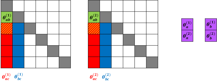
Figure 1: An illustrative example with $L=K=2$, $p=6$, and $(a,b)=(1,2)$. The green cells are the parameters of interest: $\left\{\theta_{ab}^{(l)}\right\}_{l\in[L]}$; the red cells represent $\left\{\theta_{ac}^{(l)}\right\}_{l\in[2],c\in-ab}$; the blue cells represent $\left\{\theta_{bc}^{(l)}\right\}_{l\in[2],c\in-ab}$; the purple cells represent $\left\{\theta_{a}^{(k)},\theta_{b}^{(k)}\right\}_{k\in[2]}$. These parameters constitute $\theta^{ab}\in\mathbb{R}^{s^{\prime}}$. The green and purple cells correspond to $\theta^{ab,-{\rm group}}$. The striped red cells correspond to $\theta^{ac}=\left\{\theta_{ac}^{(l)}\right\}_{l\in[2]}$ with $c=3$. Finally, the white cells are parameters not used in the estimation, while the gray cells are zero diagonal values.

We modify the three step procedure in Section 3 as follow.

Step 1:

We find a pilot estimator of $\theta^{ab}$ by solving the following program

$$\widehat{\theta}^{ab} =\arg\min_{\theta\in\mathbb{R}^{s^{\prime}}}\ \mathbb{E}_{n}\left[S^{ab}(x_{i},\theta)\right]+\lambda_{1}\bigg{(}\|\theta^{ab,-{\rm group}}\|_{1}+\sum_{c\in-ab}\Big{(}\|\theta^{ac}\|_{2}+\|\theta^{bc}\|_{2}\Big{)}\bigg{)},$$ (60)

where

$$\|\theta^{ab,-{\rm group}}\|_{1}=\sum_{l=1}^{L}|\theta_{ab}^{(l)}|+\sum_{k=1}^{K}|\theta_{a}^{(k)}|+|\theta_{b}^{(k)}|$$ (61)

and $\lambda_{1}$ is a tuning parameter. Since $L>1$, we use the group Lasso penalty to estimate $\widehat{\theta}^{ab}$. Let $\widehat{M}_{1}$ be the support of $\widehat{\theta}^{ab}$:

$$\widehat{M}_{1}={\rm supp}(\widehat{\theta}^{ab,-{\rm group}})\bigcup\{E(a,c)\mid\|\widehat{\theta}^{ac}\|_{2}\neq 0\}\bigcup\{E(b,c)\mid\|\widehat{\theta}^{bc}\|_{2}\neq 0\}.$$ (62)

Step 2:

For $l\in[L]$, let $\widehat{\gamma}^{abl}\in\mathbb{R}^{s^{\prime}-1}$ be a minimizer of

$$\sum_{l\in[L]}\frac{1}{2}\mathbb{E}_{n}\Big{[}(\varphi_{1,abl}(x_{i})-\varphi_{1,-abl}(x_{i})^{\top}\gamma^{abl})^{2}+(\varphi_{2,abl}(x_{i})-\varphi_{2,-abl}(x_{i})^{\top}\gamma^{abl})^{2}\Big{]}\\ +\lambda_{2}\bigg{(}\sum_{l\in[L]}\|\gamma^{abl,-\rm{group}}\|_{1}+\sum_{c\in-ab}\Big{(}\|\gamma^{ac}\|_{2}+\|\gamma^{bc}\|_{2}\Big{)}\bigg{)},$$ (63)

where $\lambda_{2}$ is a tuning parameter. Let $\widehat{M}_{2}$ be the union of the support of $\widehat{\gamma}^{abl}$:

$$\widehat{M}_{2}=\bigcup_{l\in[L]}{\rm supp}(\widehat{\gamma}^{abl,-{\rm group}})\bigcup\{E(a,c)\mid\|\widehat{\gamma}^{ac}\|_{2}\neq 0\}\bigcup\{E(b,c)\mid\|\widehat{\gamma}^{bc}\|_{2}\neq 0\}.$$ (64)

Step 3:

Let $\widetilde{M}=E(a,b)\cup\widehat{M}_{1}\cup\widehat{M}_{2}$. We obtain our estimator as a solution to the following program

$$\widetilde{\theta}^{ab} =\arg\min_{\theta}\ \mathbb{E}_{n}\left[S^{ab}(x_{i},\theta)\right]\qquad\text{s.t.}\quad{\rm supp}(\theta)\subseteq\widetilde{M}.$$ (65)

Our estimator of $\theta_{ab}^{[L]}$ is $\widetilde{\theta}_{ab}^{[L]}\in\mathbb{R}^{L}$, a block of $\widetilde{\theta}^{ab}$.

Asymptotic Normality.

For each $l\in[L]$, define $w_{l}^{*}\in\mathbb{R}^{s^{\prime}}$ with $w^{*}_{abl}=1$ and $w^{*}_{-abl}=-\gamma^{abl,*}$, where $\gamma^{abl,*}$ is the population version of $\widehat{\gamma}^{abl}$. Define

$$\eta_{1il}=\varphi_{1,abl}(x_{i})-\varphi_{1,-abl}(x_{i})^{\top}\gamma^{abl,*}~{}~{}~{}\text{and}~{}~{}~{}\eta_{2il}=\varphi_{2,abl}(x_{i})-\varphi_{2,-abl}(x_{i})^{\top}\gamma^{abl,*},$$ (66)

and

$$\sigma_{n,l}=\mathbb{E}_{n}\left[\eta_{1il}\varphi_{1,abl}(x_{i})+\eta_{2il}\varphi_{2,abl}(x_{i})\right].$$ (67)

Let $u^{*}_{l}=w_{l}^{*}/\sigma_{n,l}$ and $U^{*}\in\mathbb{R}^{s^{\prime}\times L}$ as the stack of $u^{*}_{l}$: $U^{*}=[u_{1}^{*},\ldots,u_{L}^{*}]$. Similar to Theorem 2, we obtain the Bahadur representation for $\widetilde{\theta}_{ab}^{[L]}\in\mathbb{R}^{L}$ as:

$$\sqrt{n}\cdot\left(\widetilde{\theta}_{ab}^{[L]}-\theta_{ab}^{*[L]}\right) =-\sqrt{n}\mathbb{E}_{n}\left[U^{*\top}\left(\Gamma(x_{i})\theta^{ab,*}+g(x_{i})\right)\right]+\Delta,$$ (68)

where $\|\Delta\|_{\infty}=\mathcal{O}\left(\phi_{\max}^{2}\phi_{\min}^{-4}\cdot\sqrt{n}\lambda_{1}\lambda_{2}m\right)$. Furthermore, under similar conditions as in Section 4, we obtain

$$\sqrt{n}\Big{(}\widetilde{\theta}_{ab}^{[L]}-\theta_{ab}^{*[L]}\Big{)}\longrightarrow_{D}N(0,V_{ab}),$$ (69)

where $V_{ab}\in\mathbb{R}^{L\times L}$ is the covariance matrix defined as $V_{ab}=\operatorname*{{\rm Var}}\big{(}U^{*\top}(\Gamma(x_{i})\theta^{ab,*}+g(x_{i}))\big{)}$. From (69) we can construct a multivariate confidence interval with asymptotically nominal coverage as before.

Simultaneous inference.

For simultaneous inference, with a fixed node $a\in V$, we would like to test the null hypothesis

$$H_{0}:\theta_{ab}^{*(l)}=\breve{\theta}_{ab}^{\,(l)}\quad\text{for all }l\in\{1,\ldots,L\}\text{ and }b\in V_{a}=\{1,\ldots,p\}\backslash\{a\},$$ (70)

for some fixed $\breve{\theta}_{ab}$ versus the alternative

$$H_{1}:\theta_{ab}^{*(l)}\neq\breve{\theta}_{ab}^{\,(l)}\quad\text{for some }l\in\{1,\ldots,L\}\text{ and }b\in V_{a}=\{1,\ldots,p\}\backslash\{a\}.$$ (71)

Again, the test involves a large number of parameters, $(p-1)L$.

First, note that we can directly apply the procedure developed in Section 6. By ignoring the covariance structure of $\theta_{ab}^{(1)},\ldots,\theta_{ab}^{(L)}$, we can directly use the Gaussian multiplier bootstrap. Specifically, for each $b\in V_{a}$, we obtain the Bahadur representation in (68). Next, we stack the resulting $p-1$ vectors into a $(p-1)L$ dimensional vector and perform the Gaussian multiplier bootstrap method to calculate the test statistic and critical values. Since $L$ is an absolute constant, all the analysis in Section 6 remains valid. However, such a procedure disregards the group structure on parameters and ignores the off-diagonal elements of the covariance matrix $V_{ab}$ when constructing the test and computing the critical values.

An alternative approach is based on the moderate deviation result for the $\chi^{2}$-test developed in Liu and Shao (2013). Here, we outline the procedure and refer to Liu and Shao (2013) for technical details. First, for each $b\in V_{a}$, we define

$$T_{nb}^{2}=n\cdot\Big{(}\widetilde{\theta}_{ab}^{[L]}-\breve{\theta}_{ab}^{[L]}\Big{)}^{\top}\cdot(V_{ab})^{-1}\cdot\Big{(}\widetilde{\theta}_{ab}^{[L]}-\breve{\theta}_{ab}^{[L]}\Big{)}.$$ (72)

It follows from (69) that the limiting distribution of $T_{nb}^{2}$ is $\chi^{2}_{L}$. Under mild conditions, Theorem 2.2 of Liu and Shao (2013) shows that

$$\frac{\mathbb{P}\left(T_{nb}^{2}\geq x^{2}\right)}{\mathbb{P}\left(\chi^{2}_{L}\geq x^{2}\right)}\rightarrow 1,\quad\text{as }n\rightarrow\infty$$

uniformly for $x\in[0,o(n^{1/6}))$. This motivates the following test statistic

$$\max_{b\in V_{a}}\,T_{nb}^{2}.$$ (73)

We obtain the critical value $y_{\alpha}$ that satisfies

$$(p-1)\cdot\mathbb{P}\left(\chi^{2}_{L}\geq y_{\alpha}\right)=-\log(1-\alpha).$$

The null hypothesis is rejected if $\max_{b\in V_{a}}T_{nb}^{2}\geq y$. We can prove that the asymptotic Type I error is $\alpha$ under the null only when the dependency among $T_{nb}^{2}$ is weak. We refer to Liu and Shao (2013) for technical details. The disadvantage of this approach is that, the terms $T_{nb}^{2}$ are correlated across $b\in V_{a}$, which is ignored when computing the critical value. Despite ignoring the group structure, the approach based on multiplier bootstrap can control the Type I error better with small sample sizes. See Section 8 for experimental results.

8 Simulations

In this section, we illustrate the finite sample properties of our inference procedure on several synthetic data sets. We generate data from four different Exponential family distributions that were introduced in Section 2.1. The first and third example involve Gaussian node-conditional distributions, for which we use regularized score matching. For the second and fourth setting where the node-conditional distributions follow Truncated Gaussian and Exponential distribution, respectively, we use regularized non-negative score matching procedure. Following the recommendation in Yu et al. (2018), we set $\ell_{a}(x)=\log(x+1)$ for the non-negative settings. In each example, we report the mean coverage rate of 95% confidence intervals for several coefficients averaged over 500 independent simulation runs.

Gaussian graphical model.

For the Gaussian setting, we have $X\sim N(0,\Sigma)$ with precision matrix $\Omega=\Sigma^{-1}=(\theta_{ab})$. Without loss of generality, say we are interested in $\theta_{12}$. We have

$$\theta^{*}=(\theta^{*}_{11},\theta^{*}_{12},\ldots,\theta^{*}_{1p},\theta^{*}_{22},\theta^{*}_{23},\ldots,\theta^{*}_{2p})^{T},$$

$$\varphi(x)=\Big{(}-\frac{1}{2}x_{1}^{2},-x_{1}x_{2},\ldots,-x_{1}x_{p},-\frac{1}{2}x_{2}^{2},-x_{2}x_{3},\ldots,-x_{2}x_{p}\Big{)}^{T},$$

$$\varphi_{1}(x)=(-x_{1},-x_{2},\ldots,-x_{p},0,\ldots,0)^{T},$$

$$\varphi_{2}(x)=(0,-x_{1},0,\ldots,0,-x_{2},-x_{3},\ldots,-x_{p})^{T},$$

$$g(x)=(-1,0,0,\ldots,0,-1,0,\ldots,0)^{T},$$

where for $g$ the second ‘$-1$’ is at location $p+1$. Now we have

$$\gamma^{ab,*} =\arg\min\ \mathbb{E}[(\varphi_{1,ab}(x_{i})-\varphi_{1,-ab}(x_{i})^{T}\gamma)^{2}+(\varphi_{2,ab}(x_{i})-\varphi_{2,-ab}(x_{i})^{T}\gamma)^{2}]$$

$$=\arg\min\ \mathbb{E}[(x_{2}-(x_{1},x_{3},\ldots,x_{p},0,\ldots,0)^{T}\gamma)^{2}+(x_{1}-(0,\ldots,0,x_{2},x_{3},\ldots,x_{p})^{T}\gamma)^{2}].$$

We can see that $\gamma^{ab,*}$ can be partitioned into first $p-1$ elements and last $p-1$ elements: $\gamma^{ab,*}=[\gamma^{ab,*}_{1};\gamma^{ab,*}_{2}]$. The two parts can be optimized separately. Moreover, both the population quantity $\varphi_{1}(x)\varphi_{1}(x)^{\top}$ and $\varphi_{2}(x)\varphi_{2}(x)^{\top}$ are the covariance matrix $\Sigma$ after rearranging terms and ignoring zero components. Assumption SE is satisfied with most of the commonly used covariance matrices with full rank. Moreover, we can verify that $\gamma^{ab,*}_{1}$ and $\gamma^{ab,*}_{2}$ are proportional to the second and first column of the precision matrix $\Omega$. Therefore, assumption M is satisfied when the columns of the precision matrix $\Omega$ are sparse.

For the experiment, we set diagonal entries of $\Omega$ as $\theta_{jj}=1$. The sparsity pattern of the precision matrix corresponds to the the 4-nearest neighbor graph and the non-zero coefficients are set as $\theta_{j,j-1}=\theta_{j-1,j}=0.5$ and $\theta_{j,j-2}=\theta_{j-2,j}=0.3$. We set the sample size $n=300$ and vary the number of nodes $p$. Table 1 shows the empirical coverage rate for different values of $p$ for four chosen coefficients. As is evident from the table, the coverage probabilities for the unknown coefficient is remarkably close to nominal.

	$\theta_{1,2}$	$\theta_{1,3}$	$\theta_{1,4}$	$\theta_{1,10}$
$p=50$	95.4%	92.4%	93.8%	93.2%
$p=200$	94.6%	92.4%	92.6%	94.0%
$p=400$	94.6%	94.8%	92.6%	93.8%

Table 1: Empirical Coverage for Gaussian Graphical Model

Non-negative Gaussian.

For simplicity we first consider score matching for non-negative Gaussian model with $\ell(x)=x^{2}$. Following the setting and notation in the previous paragraph, we have

$$\widetilde{\varphi}_{1}(x) =x_{1}\cdot\varphi_{1}(x)=x_{1}\cdot(-x_{1},-x_{2},\ldots,-x_{p},0,\ldots,0)^{T},$$

$$\widetilde{\varphi}_{2}(x) =x_{2}\cdot\varphi_{2}(x)=x_{2}\cdot(0,-x_{1},0,\ldots,0,-x_{2},-x_{3},\ldots,-x_{p})^{T}.$$

As before, $\gamma^{ab,*}$ is separable into two parts; we focus on one to obtain

$$\gamma^{ab,*}_{2}=\left[\mathbb{E}\,\,x_{1}^{2}\cdot\begin{pmatrix}x_{1}^{2}&x_{1}x_{3}&\cdots&x_{1}x_{p}\\ x_{1}x_{3}&x_{3}^{2}&\cdots&x_{3}x_{p}\\ \vdots&\vdots&\ddots&\vdots\\ x_{1}x_{p}&x_{3}x_{p}&\cdots&x_{p}^{2}\end{pmatrix}\right]^{-1}\cdot\left[\mathbb{E}\,\,x_{1}^{2}x_{2}\cdot\begin{pmatrix}x_{1}\\ x_{3}\\ \vdots\\ x_{p}\end{pmatrix}\right].$$

We can see that it contains expectations, such as $x_{1}^{2}x_{3}x_{4}$, which are hard to calculate explicitly, in addition to the matrix inversion. To the best of our knowledge, this calculation is intractable. If we instead use generalized score matching with $\ell(x)=\log(x+1)$, the calculation would be more complicated.

One exception is when the precision matrix $\Omega=I_{p}$, which means $x_{i}$ follows i.i.d. non-negative standard normal distribution. Using the moments $\mathbb{E}[x]=\sqrt{2/\pi}$, $\mathbb{E}[x^{2}]=1$, $\mathbb{E}[x^{3}]=\sqrt{8/\pi}$, $\mathbb{E}[x^{4}]=3$, we can calculate $\gamma^{ab,*}$ explicitly. It turns out that the two parts in $\gamma^{ab,*}$ are the same. All their components take the same value at approximately $1/p$, except for one component that takes the value approximately $1.6/p$. Therefore, we can see that the sparsity assumption on $\gamma^{ab,*}$ is violated. It instead only satisfies a weaker condition that $\|\gamma^{ab,*}\|_{1}\leq 2$ for large $p$. Similarly, we can calculate that $\|M^{*}_{ab}\|_{1}\leq 5$ for large $p$. We then follow the debias method in Section 5 to construct confidence intervals.

For the simulation, we use the same setting as for the Gaussian graphical model with $\theta_{j,j-1}=\theta_{j-1,j}=0.3$ and $\theta_{j,j-2}=\theta_{j-2,j}=0.1$. We set $\ell_{a}(x)=\log(x+1)$, and use the minimax tilting method to generate the data (Botev, 2017). We first support the bounded $L_{1}$ norm condition of $M^{*}$ through experiments with a small $p=20,50$ and large $n$. Here we focus on the edge $(a,b)=(1,2)$; results for other edges are similar, and are therefore omitted. Since we have enough samples, we estimate $M$ as the exact inverse of the empirical quantity $\mathbb{E}_{n}[\Gamma(x_{i}^{\prime})]$. Table 2 shows the average mean and maximum of the $L_{1}$ norm of $M$ on column $ab$, based on 500 independent simulation runs with different sample sizes. This shows that the $L_{1}$ norm of the column $ab$ of $M^{*}$ would be bounded from above. These experimental results indicate that the bounded $L_{1}$ norm condition of $M^{*}$ is reasonable.

Table 3 shows the empirical coverage rate for various choices of $p$ and $n$. Note that since we are doing sample splitting, the real sample size is $2n$. We observe that by using the debias method, we can obtain nominal coverage rate even for relatively large $p$ with small $n$.

	$n=500$	$n=2000$	$n=10000$	$n=50000$
averaged mean, $p=20$	13.01	11.42	11.16	11.10
averaged max, $p=20$	17.84	13.46	11.95	11.52
averaged mean, $p=50$	24.71	15.19	12.90	12.72
averaged max, $p=50$	32.65	17.86	14.13	13.17

Table 2: Averaged mean and max of the $L_{1}$ norm of $M$, for Non-negative Gaussian

	$\theta_{1,2}$	$\theta_{1,3}$	$\theta_{1,4}$	$\theta_{1,10}$
$p=100,n=150$	94.2%	93.8%	95.0%	92.4%
$p=200,n=300$	95.2%	96.6%	94.8%	94.6%
$p=300,n=500$	94.8%	95.8%	95.0%	94.4%

Table 3: Empirical Coverage for Non-negative Gaussian, using debias method

Normal conditionals.

For the experiment, we consider a special case of normal conditionals with $L=1$ parameter matrix, whose density is

$$p(x;B,\beta,\beta^{(2)})\propto\exp\left\{\sum_{a\neq b}\beta_{ab}x_{a}^{2}x_{b}^{2}+\sum_{a\in V}\beta_{a}^{(2)}x_{a}^{2}+\sum_{a\in V}\beta_{a}x_{a}\right\},\quad x\in\mathbb{R}^{p}.$$ (74)

This distribution is also considered in Lin et al. (2016). We set $\beta_{j}=0.4$, $\beta_{j}^{(2)}=-2$, and we use a 4 nearest neighbor lattice dependence graph with interaction matrix: $\beta_{j,j-1}=\beta_{j-1,j}=-0.2$ and $\beta_{j,j-2}=\beta_{j-2,j}=-0.2$. Since the univariate marginal distributions are all Gaussian, we generate the data using a Gibbs sampler. The first 500 samples were discarded as ‘burn in’ step, and of the remaining samples, we keep one in three.

We first support the assumption M through experiments with a small $p=20$ and large $n$. Here we focus on the edge $(a,b)=(1,2)$; results for other edges are similar, and are therefore omitted. We estimate $\widehat{\gamma}^{ab}$ as in Step 2, but without the $L_{1}$ regularization term since we have enough samples. For normal conditionals, we have $\widehat{\gamma}^{ab}\in\mathbb{R}^{2p}=\mathbb{R}^{40}$. There are five components in $\widehat{\gamma}^{ab}$ with relatively large non-zero values (not decreasing with $n$), and we calculate the mean and maximum absolute value of the remaining 35 components. Table 4 shows the average mean and maximum absolute values of these 35 components, based on 500 independent simulation runs with different sample sizes. This suggests that the population quantity $\gamma^{ab,*}$ would be close to a sparse vector, with an infinite amount of samples. These experimental results indicate that assumption M is reasonable, at least in an approximately sparse version.

We then set the number of samples $n=500$, and follow the proposed three-step procedure to calculate the coverage rate. Table 5 shows the empirical coverage rate for $p=100$ and $p=300$ nodes. Again, we see that our inference algorithm behaves well on the above Normal Conditionals Model.

	$n=500$	$n=2000$	$n=10000$	$n=50000$
average mean	$4.3\times 10^{-3}$	$2.7\times 10^{-3}$	$1.4\times 10^{-3}$	$0.7\times 10^{-3}$
average max	$9.7\times 10^{-3}$	$8.4\times 10^{-3}$	$6.9\times 10^{-3}$	$5.5\times 10^{-3}$

Table 4: Average mean and max on the 35 components, for Normal Conditionals

	$\beta_{1,2}$	$\beta_{1,3}$	$\beta_{1,4}$	$\beta_{1,10}$
$p=100$	93.2%	93.4%	94.6%	95.0%
$p=300$	93.2%	93.0%	92.6%	93.0%

Table 5: Empirical Coverage for Normal Conditionals

Exponential graphical model.

We choose $\theta_{j}=2$, and a 2 nearest neighbor dependence graph with $\theta_{j,j-1}=\theta_{j-1,j}=0.3$. We again first support the assumption M through experiment with a small $p=20$ and large $n$, where we focus on the edge $(a,b)=(1,2)$ and use a Gibbs sampler to generate data. For exponential graphical model, we have $\widehat{\gamma}^{ab}\in\mathbb{R}^{2p-2}=\mathbb{R}^{38}$. There are four components in $\widehat{\gamma}^{ab}$ with relatively large non-zero values (not decreasing with $n$), and we calculate the mean and maximum absolute value of the remaining 34 components. Table 6 shows the average mean and maximum absolute values of these 34 components, based on 500 independent simulation runs with different sample sizes. This suggests that the population quantity $\gamma^{ab,*}$ would be close to a sparse vector, with an infinite amount of samples. Once again, this experiment results indicate that assumption M is reasonable, at least in an approximately sparse version.

We then set $n=1000$ and the empirical coverage rate and histograms of estimates of four selected coefficients are presented in Table 7 and Figures 2 for $p=100$ and $p=300$, respectively.

	$n=500$	$n=2000$	$n=10000$	$n=50000$
average mean	$3.6\times 10^{-3}$	$2.2\times 10^{-3}$	$0.9\times 10^{-3}$	$0.4\times 10^{-3}$
average max	$9.4\times 10^{-2}$	$6.8\times 10^{-3}$	$3.8\times 10^{-3}$	$1.2\times 10^{-3}$

Table 6: Average mean and max on the 34 components, for Exponential Graphical Model

	$\theta_{1,2}$	$\theta_{1,3}$	$\theta_{1,4}$	$\theta_{1,10}$
$p=100$	94.2%	91.6%	92.6%	92.4%
$p=300$	92.6%	92.0%	92.2%	92.4%

Table 7: Empirical Coverage for Exponential Graphical Model

Figure 2: Histograms for $\theta$ for exponential graphical model. The first row corresponds to $p=100$ and the second row to $p=300$.

We can see from the simulations here that we need more samples for inference based on non-negative score matching to be valid, compared to regular score matching. The results are still impressive as the sample size is small relative to the total number of parameters in the model. Moreover, by using the generalized score matching with $\ell_{a}(x)=\log(x+1)$, we get more accurate empirical coverage compared to the original score matching, which uses $\ell_{a}(x)=x^{2}$. The histograms in Figures 2 show that the fitting is quite good, but to get a better estimation and hence better coverage, we would need more samples.

Simultaneous inference.

We then apply the simultaneous inference procedure to test for all the edges connected to some node $a\in V$. Since the sample complexity (41) for simultaneous inference is large, we set $p=50$. For hypothesis testing, we focus on the first node and we would like to test the null hypothesis

$$H_{0}:\theta_{1b}^{*}=\breve{\theta}_{1b}\quad\text{for all }b\in V_{1}=\{2,\ldots,p\},$$ (75)

versus the alternative

$$H_{1}:\theta_{1b}^{*}\neq\breve{\theta}_{1b}\quad\text{for some }b\in V_{1}=\{2,\ldots,p\}.$$ (76)

We set the designed Type I error as $\alpha=0.05$ and we consider Gaussian and Non-negative Gaussian settings as before. Table 8 shows the empirical Type I error under the null $\breve{\theta}_{1b}=\theta_{1b}^{*}$ with different choices of sample size. We see that our procedure works well as long as we have enough data.

	$n=500$	$n=800$	$n=1000$	$n=2000$	$n=5000$
Gaussian	0.082	0.074	0.042	0.052	0.048
Non-negative Gaussian	0.072	0.062	0.054	0.040	0.046

Table 8: Empirical Type I error of simultaneous test

Simultaneous inference with general $L$.

We finally consider the simultaneous inference with general $L$. We consider the normal conditionals model with density

$$p(x;\Theta^{(1)},\Theta^{(2)},\eta,\beta)\propto\exp\left\{\sum_{a\neq b}\Theta_{ab}^{(2)}x_{a}^{2}x_{b}^{2}+\sum_{a\neq b}\Theta_{ab}^{(1)}x_{a}x_{b}+\sum_{a\in V}\eta_{a}x_{a}^{2}+\sum_{a\in V}\beta_{a}x_{a}\right\},\,x\in\mathbb{R}^{p}.$$

This corresponds to $L=K=2$. We apply the two methods in Section 7 to test for all the edges connected to some node $a\in V$. We set $p=50$ and the designed Type I error $\alpha=0.05$. For hypothesis testing, we focus on the first node (i.e., $a=1$). Table 9 shows the empirical Type I error under the null with different choices of sample sizes. We see that both methods work well as long as we have enough data.

	$n=1000$	$n=2000$	$n=4000$	$n=6000$
Gaussian multiplier bootstrap	0.076	0.058	0.054	0.048
Moderate deviation method	0.182	0.092	0.068	0.056

Table 9: Empirical Type I error of simultaneous test with general $L$

9 Protein Signaling Dataset

In this section we apply our algorithm to a protein signaling flow cytometry data set, which contains the presence of $p=11$ proteins in $n=7466$ cells (Sachs et al., 2005). Yang et al. (2015) fit exponential and Gaussian graphical models to the data set.

Figure 3 shows the network structure after applying our method to the data using an Exponential Graphical Model. We learn the structure directly from the data as well as provide confidence intervals using the Exponential Graphical Model, rather than log-transforming the data and fitting Gaussian graphical model as was done in Yang et al. (2015). To infer the network structure, we calculate the $p$-value for each pair of nodes, and keep the edges with $p$-values smaller than 0.01. Estimated negative conditional dependencies are shown via red edges. Recall that the exponential graphical model restricts the edge weights to be non-negative, hence only negative dependencies can be estimated. From the figure we see that PKA is a major protein inhibitor in cell signaling networks. This result is consistent with the estimated graph structure in Yang et al. (2015), as well as in the Bayesian network of Sachs et al. (2005). In addition, we find significant dependency between PKC and PIP3.

Figure 3: Estimated Structure of Protein Signaling Dataset

10 Conclusion

Motivated by applications in Biology and Social Networks, much progress has been made in statistical learning models and methods for networks with a large number of nodes. Graphical models provide a powerful and flexible modeling framework for such networks to uncover the dependency among nodes. As a result, there is a vast literature on estimation and inference algorithms for high dimensional Gaussian graphical models, as well as more general graphical models in the exponential family. As a disadvantage of most of these works, the normalizing constant (partition function) of the conditional densities is usually computationally intractable and without closed-form formula. Score matching estimators provide a way to address this issue, but so far all the existing works on score matching focus on estimation problem for high-dimensional graphical models without statistical inference. In this paper, we fill this gap by proposing a novel estimator using the score matching method that is asymptotically normal, which allows us to build statistical inference for a single edge of the graph. Moreover, we propose the procedure on simultaneous testing on all the edges connected to some specific node in the graph, using the Gaussian multiplier bootstrap method. This procedure can be used to test if certain nodes are isolated or not, recover the support of the graph, and test the difference between two graphical models. There are a number of interesting and important directions that will be explored in future. For example, developing inferential techniques based on score matching for multi-attribute graphical models (Kolar et al., 2013, 2014), graphical models with confounders (Geng et al., 2019, 2018), time-varying graphical models (Zhou et al., 2010; Kolar et al., 2010b; Kolar and Xing, 2011), networks with jumps (Kolar and Xing, 2012) and conditional graphical models (Kolar et al., 2010a), as well as data with missing values (Kolar et al., 2010a). It is also of interest to incorporate constraints in the model and perform constrained inference (Yu et al., 2020). Finally, our method is developed for continuous data and developing results for discrete valued data is also of interest.

Acknowledgments

We are extremely grateful to the associate editor, Jie Peng, and two anonymous reviewers for their insightful comments that helped improve this paper. This work is partially supported by an IBM Corporation Faculty Research Fund and the William S. Fishman Faculty Research Fund at the University of Chicago Booth School of Business. This work was completed in part with resources provided by the University of Chicago Research Computing Center.

A Technical proofs

We first establish a bound on the size of $\widehat{m}_{1}=\left|\widehat{M}_{1}\right|$ and $\widehat{m}_{2}=\left|\widehat{M}_{2}\right|$ in the following lemma.

Lemma 9

Assume the conditions of Theorem 2 are satisfied. Then

$$\widehat{m}_{1}+\widehat{m}_{2}\lesssim\phi_{\max}\phi_{\min}^{-2}m.$$

Proof  From the KKT conditions we have that $\widehat{\theta}^{ab}$ satisfies

$$\mathbb{E}_{n}\left[\Gamma(x_{i})\widehat{\theta}^{ab}+g(x_{i})\right]+\lambda_{1}\cdot\widehat{\tau}=0,$$

where $\widehat{\tau}\in\partial\|\widehat{\theta}^{ab}\|_{1}$. Restricted to $\widehat{M}_{1}$, we have (elementwise)

$$\left|\left(\mathbb{E}_{n}\left[\Gamma(x_{i})\widehat{\theta}^{ab}+g(x_{i})\right]\right)_{\widehat{M}_{1}}\right|=\lambda_{1}.$$

Computing the $\ell_{2}$ norm on both sides,

$$\sqrt{\widehat{m}_{1}}\cdot\lambda_{1} =\bigg{\|}\left(\mathbb{E}_{n}\left[\Gamma(x_{i})\widehat{\theta}^{ab}+g(x_{i})\right]\right)_{\widehat{M}_{1}}\bigg{\|}_{2}$$

$$\leq\bigg{\|}\left(\mathbb{E}_{n}\left[\Gamma(x_{i})\left(\widehat{\theta}^{ab}-\theta^{ab,*}\right)\right]\right)_{\widehat{M}_{1}}\bigg{\|}_{2}+\bigg{\|}\left(\mathbb{E}_{n}\left[\Gamma(x_{i})\theta^{ab,*}+g(x_{i})\right]\right)_{\widehat{M}_{1}}\bigg{\|}_{2}$$

$$\triangleq L_{1}+L_{2}.$$

For the first term we have that

$$L_{1} \leq\phi_{+}(\widehat{m}_{1}+m,\mathbb{E}_{n}\left[\Gamma(x_{i})\right])\cdot r_{2\theta}$$

$$\lesssim\phi_{+}(\widehat{m}_{1}+m,\mathbb{E}_{n}\left[\Gamma(x_{i})\right])\cdot\phi_{\min}^{-1}\cdot\lambda_{1}\sqrt{m},$$

using Negahban et al. (2012). For the second term, we have that

$$L_{2}\leq\sqrt{\widehat{m}_{1}}\cdot\lambda_{1}/2.$$

Combining the two bounds, we obtain

$$\sqrt{\widehat{m}_{1}}\lesssim\phi_{+}(\widehat{m}_{1}+m,\mathbb{E}_{n}\left[\Gamma(x_{i})\right])\cdot\phi_{\min}^{-1}\sqrt{m}.$$

Now, proceeding as in the proof of Theorem 3 in Belloni and Chernozhukov (2013), we establish that

$$\widehat{m}_{1}\lesssim\phi_{\max}\phi_{\min}^{-2}m.$$

The proof for $\widehat{m}_{2}$ is similar.  

Our next result establishes bounds on $\widetilde{\theta}^{ab}-\theta^{ab,*}$.

Lemma 10

Assume the conditions of Theorem 2 are satisfied. Then

$$\|\widetilde{\theta}^{ab}-\theta^{ab,*}\|_{2} \lesssim\phi_{\max}^{1/2}\phi_{\min}^{-2}\cdot\lambda_{1}\sqrt{m},$$

$$\|\widetilde{\theta}^{ab}-\theta^{ab,*}\|_{1} \lesssim\phi_{\max}^{1/2}\phi_{\min}^{-2}\cdot\lambda_{1}m.$$

Proof  From the KKT conditions we have that $\widehat{\theta}^{ab}$ satisfies

$$\mathbb{E}_{n}\left[\Gamma(x_{i})_{\widehat{M}_{1}}\right]\widehat{\theta}^{ab}_{\widehat{M}_{1}}+\mathbb{E}_{n}\left[g(x_{i})_{\widehat{M}_{1}}\right]+\lambda_{1}\cdot{\rm sign}(\widehat{\theta}^{ab}_{\widehat{M}_{1}})=0,$$

while $\widetilde{\theta}^{ab}$ satisfies

$$\mathbb{E}_{n}\left[\Gamma(x_{i})_{\widetilde{M}}\right]\widetilde{\theta}^{ab}_{\widetilde{M}}+\mathbb{E}_{n}\left[g(x_{i})_{\widetilde{M}}\right]=0.$$

Combining these two equations we have

$$\mathbb{E}_{n}\left[\Gamma(x_{i})_{\widetilde{M}}\right]\left(\widetilde{\theta}^{ab}_{\widetilde{M}}-\widehat{\theta}^{ab}_{\widehat{M}_{1}}\right)=\lambda_{1}\cdot{\rm sign}(\widehat{\theta}^{ab}_{\widehat{M}_{1}})$$

and

$$\phi_{\min}\cdot\|\widetilde{\theta}^{ab}_{\widetilde{M}}-\widehat{\theta}^{ab}_{\widehat{M}_{1}}\|_{2}\leq\bigg{\|}\mathbb{E}_{n}\left[\Gamma(x_{i})_{\widetilde{M}}\right]\left(\widetilde{\theta}^{ab}_{\widetilde{M}}-\widehat{\theta}^{ab}_{\widehat{M}_{1}}\right)\bigg{\|}_{2}=\lambda_{1}\sqrt{\widehat{m}_{1}}.$$

Therefore, using Negahban et al. (2012),

$$\|\widetilde{\theta}^{ab}-\theta^{ab,*}\|_{2}\leq\|\widetilde{\theta}^{ab}-\widehat{\theta}^{ab,*}\|_{2}+\|\widehat{\theta}^{ab}-\theta^{ab,*}\|_{2}\lesssim\phi_{\min}^{-1}\cdot\lambda_{1}\sqrt{\widehat{m}_{1}}.$$

Combining with Lemma 9, we obtain

$$\|\widetilde{\theta}^{ab}-\theta^{ab,*}\|_{2}\lesssim\phi_{\max}^{1/2}\phi_{\min}^{-2}\cdot\lambda_{1}\sqrt{m}\quad\text{and}\quad\|\widetilde{\theta}^{ab}-\theta^{ab,*}\|_{1}\lesssim\phi_{\max}^{1/2}\phi_{\min}^{-2}\cdot\lambda_{1}m.$$

 

A similar result can be established for $\widetilde{\gamma}^{ab}-\gamma^{ab,*}$, which we state without proof, as it is analogous to the proof of Lemma 10.

Lemma 11

Assume the conditions of Theorem 2 are satisfied. Then

$$\|\widetilde{\gamma}^{ab}-\gamma^{ab,*}\|_{2} \lesssim\phi_{\max}^{1/2}\phi_{\min}^{-2}\cdot\lambda_{2}\sqrt{m},$$

$$\|\widetilde{\gamma}^{ab}-\gamma^{ab,*}\|_{1} \lesssim\phi_{\max}^{1/2}\phi_{\min}^{-2}\cdot\lambda_{2}m.$$

To simplify notation later, let $\widetilde{r}_{j\theta}=\|\widetilde{\theta}^{ab}-\theta^{ab,*}\|_{j}$ and $\widetilde{r}_{j\gamma}=\|\widetilde{\gamma}^{ab}-\gamma^{ab,*}\|_{j}$, for $j\in\{1,2\}$.

Lemma 12

Under the conditions of Theorem 2, we have

$$\left|\left(\widetilde{w}-w^{*}\right)^{\top}\mathbb{E}_{n}\left[\Gamma(x_{i})\right]\left(\widetilde{\theta}^{ab}-\theta^{ab,*}\right)\right|\lesssim\phi_{\max}^{2}\phi_{\min}^{-4}\cdot\lambda_{1}\lambda_{2}{m}.$$

Proof  Let ${\mathcal{S}}_{k}$ be the set of $k$-sparse vectors in the unit ball,

$${\mathcal{S}}_{k}=\left\{u\in\mathbb{R}^{p}:\|u\|_{2}\leq 1,\|u\|_{0}\leq k\right\}.$$

Abusing the notation, let $\|\cdot\|_{{\mathcal{S}}_{k}}$ denote the sparse spectral norm for matrices, that is,

$$\|M\|_{{\mathcal{S}}_{k}}=\max_{u,v\in{\mathcal{S}}_{k}}u^{\top}Mv.$$

Using Lemma 4.9 of Barber and Kolar (2018),

$$|u^{\top}Mv|\leq\left(\|u\|_{2}+\|u\|_{1}/\sqrt{k}\right)\cdot\left(\|v\|_{2}+\|v\|_{1}/\sqrt{k}\right)\cdot\sup_{u^{\prime},v^{\prime}\in{\mathcal{S}}_{k}}|u^{\prime\top}Mv^{\prime}|$$

for any fixed matrix $M\in\mathbb{R}^{p\times p}$ and vectors $u,v\in\mathbb{R}^{p}$, and any $k\geq 1$. With this, we have

$$\left(\widetilde{w}-w^{*}\right)^{\top}\mathbb{E}_{n}\left[\Gamma(x_{i})\right]\left(\widetilde{\theta}^{ab}-\theta^{ab,*}\right) \leq\|\mathbb{E}_{n}\left[\Gamma(x_{i})\right]\|_{{\mathcal{S}}_{\widetilde{m}}}\cdot\left(\widetilde{r}_{2\gamma}+\widetilde{r}_{1\gamma}/\sqrt{\widetilde{m}}\right)\cdot\left(\widetilde{r}_{2\theta}+\widetilde{r}_{1\theta}/\sqrt{\widetilde{m}}\right)$$

$$\lesssim\phi_{\max}^{2}\phi_{\min}^{-4}\cdot\lambda_{1}\lambda_{2}m,$$

where the second line follows from the assumption SE, and Lemma 10 and Lemma 11.  

Lemma 13

Under the conditions of Theorem 2, we have

$$\left|\left(\widetilde{w}-w^{*}\right)^{\top}\left(\mathbb{E}_{n}\left[\Gamma(x_{i})\right]\theta^{ab,*}+\mathbb{E}_{n}[g(x_{i})]\right)\right|\lesssim\phi_{\max}^{1/2}\phi_{\min}^{-2}\cdot\lambda_{1}\lambda_{2}m.$$

Proof  Using Hölder’s inequality, we have

$$\left|\left(\widetilde{w}-w^{*}\right)^{\top}\left(\mathbb{E}_{n}\left[\Gamma(x_{i})\right]\theta^{ab,*}+\mathbb{E}_{n}[g(x_{i})]\right)\right|\leq\widetilde{r}_{1\gamma}\cdot\|\mathbb{E}_{n}\left[\Gamma(x_{i})\right]\theta^{ab,*}+\mathbb{E}_{n}[g(x_{i})]\|_{\infty}.$$

On the event $\mathcal{E}_{\theta}$, we have $\|\mathbb{E}_{n}\left[\Gamma(x_{i})\right]\theta^{ab,*}+\mathbb{E}_{n}[g(x_{i})]\|_{\infty}\leq\lambda_{1}/2$. Finally, using Lemma 11, we conclude that

$$\left|\left(\widetilde{w}-w^{*}\right)^{\top}\left(\mathbb{E}_{n}\left[\Gamma(x_{i})\right]\theta^{ab,*}+\mathbb{E}_{n}[g(x_{i})]\right)\right|\lesssim\phi_{\max}^{1/2}\phi_{\min}^{-2}\cdot\lambda_{1}\lambda_{2}m.$$

 

Lemma 14

Under the conditions of Theorem 2, we have

$$w^{*\top}\mathbb{E}_{n}\left[\Gamma(x_{i})\right]\left(\widetilde{\theta}^{ab}-\theta^{ab,*}\right)=\mathbb{E}_{n}\left[\eta_{1i}\varphi_{1,ab}(x_{i})+\eta_{2i}\varphi_{2,ab}(x_{i})\right] \left(\widetilde{\theta}_{ab}-\theta_{ab}^{ab,*}\right)$$

$$+\mathcal{O}\left(\phi_{\max}^{1/2}\phi_{\min}^{-2}\cdot\lambda_{1}\lambda_{2}m\right).$$

Proof  We have that

$$w^{*\top}\mathbb{E}_{n}\left[\Gamma(x_{i})\right]\left(\widetilde{\theta}^{ab}-\theta^{ab,*}\right) =\mathbb{E}_{n}\left[\left(\eta_{1i}\varphi_{1}(x_{i})+\eta_{2i}\varphi_{2}(x_{i})\right)^{\top}\right]\left(\widetilde{\theta}^{ab}-\theta^{ab,*}\right)$$

$$=\mathbb{E}_{n}\left[\eta_{1i}\varphi_{1,ab}(x_{i})+\eta_{2i}\varphi_{2,ab}(x_{i})\right]\left(\widetilde{\theta}_{ab}^{ab}-\theta_{ab}^{ab,*}\right)$$

$$\quad+\mathbb{E}_{n}\left[\left(\eta_{1i}\varphi_{1,-ab}(x_{i})+\eta_{2i}\varphi_{2,-ab}(x_{i})\right)^{\top}\right]\left(\widetilde{\theta}_{-ab}^{ab}-\theta_{-ab}^{ab,*}\right).$$

For the second term, we have

$$\left|\mathbb{E}_{n}\left[\left(\eta_{1i}\varphi_{1,-ab}(x_{i})+\eta_{2i}\varphi_{2,-ab}(x_{i})\right)^{\top}\right]\left(\widetilde{\theta}_{-ab}^{ab}-\theta_{-ab}^{ab}\right)\right|$$

$$\qquad\leq\widetilde{r}_{1\theta}\cdot\|\mathbb{E}_{n}\left[\eta_{1i}\varphi_{1,-ab}(x_{i})+\eta_{2i}\varphi_{2,-ab}(x_{i})\right]\|_{\infty}$$

$$\qquad\leq\widetilde{r}_{1\theta}\cdot\lambda_{2}/2,$$

since we are working on the event $\mathcal{E}_{\gamma}$. Since $\widetilde{r}_{1\theta}\leq\phi_{\max}^{1/2}\phi_{\min}^{-2}\cdot\lambda_{1}m$, combining with the display above, the proof is complete.  

Lemma 15

Under the assumptions M and R, we have that

$$\sqrt{n}\cdot w^{*\top}\left(\mathbb{E}_{n}\left[\Gamma(x_{i})\theta^{ab,*}+g(x_{i})\right]\right)\longrightarrow_{D}N\left(0,H(\theta^{*})\right),$$

where $H(\theta^{*})=\operatorname*{{\rm Var}}\left(w^{*\top}\left({\Gamma(x_{i})\theta^{ab,*}+g(x_{i})}\right)\right)$.

Proof  Let $Z_{i}=w^{*\top}\left(\Gamma(x_{i})\theta^{ab,*}+g(x_{i})\right)$. Then

$$\sqrt{n}\cdot w^{*\top}\left(\mathbb{E}_{n}\left[\Gamma(x_{i})\theta^{ab,*}+g(x_{i})\right]\right)=\frac{1}{\sqrt{n}}\sum_{i}Z_{i}.$$ (77)

From Forbes and Lauritzen (2015), we have that $\mathbb{E}[Z_{i}]=0$ and $\operatorname*{{\rm Var}}(Z_{i})$ is finite. An application of the central limit theorem completes the proof.  

Lemma 16

The variance estimator $\widehat{V}_{ab}$ is consistent, $\widehat{V}_{ab}\rightarrow_{P}V_{ab}$.

Proof  The variance estimator is obtained by using the second sample moment, and replacing true $\theta^{ab,*},\gamma^{ab,*}$ with $\widetilde{\theta}^{ab},\widetilde{\gamma}^{ab}$. We show the consistency of $\widehat{V}_{ab}$ by showing the consistency of the estimator for $\sigma_{n}$ and $\text{Var}\big{(}w^{*,T}(\Gamma(x_{i})\theta^{ab,*}+g(x_{i}))\big{)}$, respectively.

Step 1.

We can write

$$\sigma_{n} =\mathbb{E}_{n}\big{[}\eta_{1i}\varphi_{1,ab}(x_{i})+\eta_{2i}\varphi_{2,ab}(x_{i})\big{]}$$

$$=\mathbb{E}_{n}\big{[}w^{*,\top}\varphi_{1}(x_{i})\cdot\varphi_{1,ab}(x_{i})+w^{*,\top}\varphi_{2}(x_{i})\cdot\varphi_{2,ab}(x_{i})]$$

$$=w^{*\top}\cdot\mathbb{E}_{n}[\Gamma(x_{i})]\cdot e_{ab}.$$

Let $\sigma=\mathbb{E}[\sigma_{n}]=w^{*\top}\cdot\mathbb{E}[\Gamma(x_{i})]\cdot e_{ab}$ denote the population version of $\sigma_{n}$ and $\widetilde{\sigma}_{n}=\widetilde{w}^{\top}\cdot\mathbb{E}_{n}[\Gamma(x_{i})]\cdot e_{ab}$ the sample version. With high probability we have that

$$|\widetilde{\sigma}_{n}-\sigma| \leq|\widetilde{\sigma}_{n}-\sigma_{n}|+|\sigma_{n}-\sigma|$$

$$\leq\Big{|}(\widetilde{w}-w^{*})^{\top}\cdot\mathbb{E}_{n}[\Gamma(x_{i})]\cdot e_{ab}\Big{|}+\Big{|}{w^{*}}^{\top}\cdot\big{[}\mathbb{E}_{n}[\Gamma(x_{i})]-\mathbb{E}[\Gamma(x_{i})]\big{]}\cdot e_{ab}\Big{|}$$

$$\leq\|\widetilde{w}-w^{*}\|_{1}\cdot\big{\|}\mathbb{E}_{n}[\Gamma(x_{i})]\cdot e_{ab}\big{\|}_{\infty}+\|w^{*}\|_{1}\cdot\big{\|}\big{[}\mathbb{E}_{n}[\Gamma(x_{i})]-\mathbb{E}[\Gamma(x_{i})]\big{]}\cdot e_{ab}\big{\|}_{\infty}$$

$$\lesssim\lambda_{2}m\cdot(C+\sqrt{\log p/n})+m\cdot\sqrt{\log p/n}=o_{P}(1).$$

Step 2.

We estimate the variance of $w^{*\top}\big{(}\Gamma(x_{i})\theta^{ab,*}+g(x_{i})\big{)}$. Since

$$\mathbb{E}\left[w^{*\top}\big{(}\Gamma(x_{i})\theta^{ab,*}+g(x_{i})\big{)}\right]=0,$$

we can use the second sample moment to estimate the variance. As above, we plug in $\widetilde{\theta}^{ab}$ and $\widetilde{\gamma}^{ab}$, to obtain that

$$\Bigg{|}\mathbb{E}_{n}\bigg{\{}\widetilde{w}^{\top}\Big{(}\Gamma(x_{i})\widetilde{\theta}^{ab}+g(x_{i})\Big{)}\bigg{\}}^{2}-\mathbb{E}_{n}\bigg{\{}w^{*\top}\Big{(}\Gamma(x_{i})\theta^{ab,*}+g(x_{i})\Big{)}\bigg{\}}^{2}\Bigg{|}$$

$$\qquad=\Bigg{|}\mathbb{E}_{n}\bigg{\{}\widetilde{w}^{\top}\big{(}\Gamma(x_{i})\widetilde{\theta}^{ab}+g(x_{i})\big{)}-w^{*\top}\big{(}\Gamma(x_{i})\theta^{ab,*}+g(x_{i})\big{)}\bigg{\}}$$

$$\qquad\quad\quad\quad\quad\quad\quad\cdot\bigg{\{}\widetilde{w}^{\top}\big{(}\Gamma(x_{i})\widetilde{\theta}^{ab}+g(x_{i})\big{)}+w^{*\top}\big{(}\Gamma(x_{i})\theta^{ab,*}+g(x_{i})\big{)}\bigg{\}}\Bigg{|}$$

$$\qquad\lesssim\mathbb{E}_{n}\bigg{|}\widetilde{w}^{\top}\left(\Gamma(x_{i})\widetilde{\theta}^{ab}+g(x_{i})\right)-w^{*\top}\left(\Gamma(x_{i})\theta^{ab,*}+g(x_{i})\right)\bigg{|}$$

$$\qquad\lesssim\mathbb{E}_{n}\bigg{|}(\widetilde{w}-w^{*})^{\top}\left(\Gamma(x_{i})\theta^{ab,*}+g(x_{i})\right)+\widetilde{w}^{\top}\Gamma(x_{i})(\widetilde{\theta}^{ab}-\theta^{ab,*})\bigg{|}$$

$$\qquad\lesssim{\|\widetilde{w}-w^{*}\|_{1}\cdot\mathbb{E}_{n}\Big{\|}\Gamma(x_{i})\theta^{ab,*}+g(x_{i})\Big{\|}_{\infty}+\|\widetilde{\theta}^{ab}-\theta^{ab,*}\|_{1}\cdot\mathbb{E}_{n}\Big{\|}\widetilde{w}^{\top}\Gamma(x_{i})\Big{\|}_{\infty}}$$

$$\qquad=o_{P}(1).$$

Combining the results of the two steps, completes the proof.  

Proof of Theorem 6

Denote

$$W_{0}=\max_{b\in V_{a}}\frac{1}{\sqrt{n}}\sum_{i=1}^{n}z_{iab}e_{i}$$ (78)

as the counterpart to $\widetilde{W}$. Let

$$T_{0}=\max_{b\in V_{a}}\frac{1}{\sqrt{n}}\sum_{i=1}^{n}z_{iab}\quad\text{and}\quad\widetilde{T}=\max_{b\in V_{a}}\frac{1}{\sqrt{n}}\sum_{i=1}^{n}\widetilde{z}_{iab}.$$ (79)

Denote

$$\Delta=\max_{b,c\in V_{a}}\bigg{|}\frac{1}{n}\sum_{i=1}^{n}\gamma_{abc}(x_{i})\bigg{|},$$ (80)

where $\gamma_{abc}(x_{i})$ is defined in assumption RR. In order to apply Theorem 3.2 in Chernozhukov et al. (2013), we check the following conditions:

1. $\mathbb{P}(\Delta\geq n^{-c})\leq n^{-c}$.

2. $\mathbb{P}(|T_{0}-\widetilde{T}|\geq n^{-c})\leq p^{-c}$.

3. With probability at least $1-p^{-c}$, $\mathbb{P}_{e}(|W_{0}-\widetilde{W}|\geq n^{-c})\leq n^{-c}$. Here $\mathbb{P}_{e}$ denotes the probability with respect to $\{e_{i}\}_{i=1}^{n}$, conditionally on the observed data.

We verify the first condition by applying Lemma A.1 in van de Geer (2008). By the definition of $\gamma_{abc}(x_{i})$, clearly we have $\mathbb{E}\left[\gamma_{abc}(x_{i})\right]=0$. Together with assumption RR, we apply Lemma A.1 in van de Geer (2008) and obtain

$$\mathbb{E}[\Delta]\leq\sqrt{\frac{4\tau_{n}^{2}\log{(2p)}}{n}}+\frac{2\eta_{n}\log{(2p)}}{n}.$$

According to (41), for sufficiently large $n$, we have $\mathbb{E}[\Delta]\leq n^{-2c}$, for some $c>0$. By Markov inequality,

$$\mathbb{P}(\Delta\geq n^{-c})\leq n^{c}\cdot\mathbb{E}[\Delta]\leq n^{-c},$$

which verifies the first condition.

Next, we verify the second condition. For a fixed $b\in V_{a}$, under the null, we have

$$\bigg{|}\frac{1}{\sqrt{n}}\sum_{i=1}^{n}z_{iab}-\frac{1}{\sqrt{n}}\sum_{i=1}^{n}\widetilde{z}_{iab}\bigg{|} \leq\sqrt{n}\bigg{|}(\sigma_{ab}^{-1}-\sigma_{n,ab}^{-1})\cdot w_{ab}^{*\top}\Big{(}\mathbb{E}_{n}\big{[}\Gamma_{ab}(x_{i})\theta^{ab,*}+g_{ab}(x_{i})\big{]}\Big{)}\bigg{|}$$

$$\qquad+\sqrt{n}\bigg{|}\sigma_{n,ab}^{-1}\cdot(w_{ab}^{*}-\widetilde{w}_{ab})^{\top}\Big{(}\mathbb{E}_{n}\big{[}\Gamma_{ab}(x_{i})\theta^{ab,*}+g_{ab}(x_{i})\big{]}\Big{)}\bigg{|}$$

$$\leq\sqrt{n}C\cdot\lambda_{1}\lambda_{2}m$$

$$\leq n^{-c},$$

with probability at least $1-p^{-c-1}$, where the second inequality comes from the consistency of $\sigma_{n}$, Lemma 13, and Lemma 15. We then have

$$\mathbb{P}(|T_{0}-\widetilde{T}|\geq n^{-c}) \leq\mathbb{P}\Big{(}\bigcup_{b\in V_{a}}\Big{\{}\frac{1}{\sqrt{n}}\big{|}\sum_{i=1}^{n}z_{iab}-\sum_{i=1}^{n}\widetilde{z}_{iab}\big{|}\geq n^{-c}\Big{\}}\Big{)}$$

$$\leq\sum_{b\in V_{a}}\mathbb{P}\Big{(}\frac{1}{\sqrt{n}}\big{|}\sum_{i=1}^{n}z_{iab}-\sum_{i=1}^{n}\widetilde{z}_{iab}\big{|}\geq n^{-c}\Big{)}$$

$$\leq p\cdot p^{-c-1}=p^{-c},$$

which verifies the second condition.

Finally, we verify the third condition. We have

$$\mathbb{P}_{e}(|W_{0}-\widetilde{W}|\geq n^{-c}) \leq\mathbb{P}_{e}\Big{(}\max_{b\in V_{a}}\Big{\{}\frac{1}{\sqrt{n}}\big{|}\sum_{i=1}^{n}(z_{iab}-\widetilde{z}_{iab})e_{i}\big{|}\Big{\}}\geq n^{-c}\Big{)}.$$ (81)

Denote $Z_{b}=\frac{1}{\sqrt{n}}\sum_{i=1}^{n}(z_{iab}-\widetilde{z}_{iab})e_{i}$. Under the null we have

$$z_{iab}-\widetilde{z}_{iab} =\Big{[}(\sigma_{ab}^{-1}-\sigma_{n,ab}^{-1})\cdot w_{ab}^{*\top}\big{(}\Gamma_{ab}(x_{i})\theta^{ab,*}+g_{ab}(x_{i})\big{)}\Big{]}$$

$$\qquad\qquad\qquad+\Big{[}\sigma_{n,ab}^{-1}\cdot(w_{ab}^{*}-\widetilde{w}_{ab})^{\top}\big{(}\Gamma_{ab}(x_{i})\theta^{ab,*}+g_{ab}(x_{i})\big{)}\Big{]}.$$

According to Lemma A.1 in Chernozhukov et al. (2013), we have

$$\mathbb{E}\bigg{[}\frac{1}{n}\Big{\|}\sum_{i=1}^{n}\Big{(}\Gamma_{ab}(x_{i})\theta^{ab,*}+g_{ab}(x_{i})\Big{)}e_{i}\Big{\|}_{\infty}\bigg{]}\lesssim\sigma_{0}\sqrt{\frac{\log p}{n}}+\frac{M\log p}{n},$$

uniformly for each $b\in V_{a}$, where

$$\sigma_{0}^{2}=\max_{j}\frac{1}{n}\sum_{i=1}^{n}\Big{[}\Big{(}\Gamma_{ab}(x_{i})\theta^{ab,*}+g_{ab}(x_{i})\Big{)}e_{i}\Big{]}_{j}^{2},$$ (82)

and

$$M^{2}=\mathbb{E}\bigg{[}\max_{i}\Big{\|}\Big{(}\Gamma_{ab}(x_{i})\theta^{ab,*}+g_{ab}(x_{i})\Big{)}e_{i}\Big{\|}_{\infty}\bigg{]}^{2}.$$ (83)

We then have

$$\mathbb{E}|Z_{b}| \leq\frac{1}{\sqrt{n}}\Big{(}(\sigma_{ab}^{-1}-\sigma_{n,ab}^{-1})\cdot\|w_{ab}^{*}\|_{1}+\sigma_{n,ab}^{-1}\cdot\|w_{ab}^{*}-\widetilde{w}_{ab}\|_{1}\Big{)}$$

$$\qquad\qquad\times\mathbb{E}\bigg{[}\Big{\|}\sum_{i=1}^{n}\Big{(}\Gamma_{ab}(x_{i})\theta^{ab,*}+g_{ab}(x_{i})\Big{)}e_{i}\Big{\|}_{\infty}\bigg{]}$$

$$\leq\frac{C}{\sqrt{n}}\cdot\lambda m\cdot\bigg{(}\sigma_{0}\sqrt{\frac{\log p}{n}}+\frac{M\log p}{n}\bigg{)}\cdot n$$

$$\leq n^{-2c},$$

uniformly for each $b\in V_{a}$ with probability at least $1-p^{-c}$, where the second inequality comes from the consistency of $\sigma_{n}$ and Lemma 11. Applying Markov inequality again, we obtain

$$\mathbb{P}_{e}(|Z_{b}|\geq n^{-c})\leq n^{c}\cdot\mathbb{E}|Z_{b}|\leq n^{-c}.$$

uniformly for each $b\in V_{a}$ with probability at least $1-p^{-c}$. Plugging back to (81), we obtain

$$\mathbb{P}_{e}(|W_{0}-\widetilde{W}|\geq n^{-c}) \leq\mathbb{P}_{e}\Big{(}\max_{b\in V_{a}}|Z_{b}|\geq n^{-c}\Big{)}\leq n^{-c}$$ (84)

with probability at least $1-p^{-c}$, which verifies the third condition.

With the three conditions verified and assumption RR, we apply Theorem 3.2 in Chernozhukov et al. (2013) to obtain

$$\sup_{\alpha\in(0,1)}\bigg{|}\mathbb{P}\Big{(}\max_{b\in V_{a}}\sqrt{n}(\widetilde{\theta}_{ab}-\breve{\theta}_{ab})\geq c_{\widetilde{W}}(\alpha)\Big{)}-\alpha\bigg{|}=o(1),$$

which completes the proof.

References

• Arnold et al. (1999) B. C. Arnold, E. Castillo, and J. M. Sarabia. Conditional specification of statistical models. Springer Series in Statistics. Springer-Verlag, New York, 1999.
• Bahadur (1966) R. R. Bahadur. A note on quantiles in large samples. Ann. Math. Statist., 37:577–580, 1966.
• Barber and Kolar (2018) R. F. Barber and M. Kolar. Rocket: Robust confidence intervals via kendall’s tau for transelliptical graphical models. Ann. Statist., 46(6B):3422–3450, 2018.
• Belloni and Chernozhukov (2013) A. Belloni and V. Chernozhukov. Least squares after model selection in high-dimensional sparse models. Bernoulli, 19(2):521–547, 2013.
• Belloni et al. (2013) A. Belloni, V. Chernozhukov, and C. B. Hansen. Inference on treatment effects after selection amongst high-dimensional controls. Rev. Econ. Stud., 81(2):608–650, 2013.
• Botev (2017) Z. I. Botev. The normal law under linear restrictions: simulation and estimation via minimax tilting. J. R. Stat. Soc. Ser. B. Stat. Methodol., 79(1):125–148, 2017.
• Cai et al. (2011) T. T. Cai, W. Liu, and X. Luo. A constrained $\ell_{1}$ minimization approach to sparse precision matrix estimation. J. Am. Stat. Assoc., 106(494):594–607, 2011.
• Cao and Dowd (2019) J. Cao and C. Dowd. Estimation and inference for synthetic control methods with spillover effects. arXiv preprint arXiv:1902.07343, 2019.
• Cao and Lu (2019) J. Cao and S. Lu. Synthetic control inference for staggered adoption: Estimating the dynamic effects of board gender diversity policies. arXiv preprint arXiv:1912.06320, 2019.
• Chang et al. (2018) J. Chang, Y. Qiu, Q. Yao, and T. Zou. Confidence regions for entries of a large precision matrix. Journal of Econometrics, 206(1):57–82, 2018.
• Chen et al. (2015) S. Chen, D. M. Witten, and A. Shojaie. Selection and estimation for mixed graphical models. Biometrika, 102(1):47–64, 2015.
• Cheng et al. (2013) J. Cheng, E. Levina, and J. Zhu. High-dimensional mixed graphical models. ArXiv e-prints, arXiv:1304.2810, 2013, arXiv:1304.2810.
• Chernozhukov et al. (2013) V. Chernozhukov, D. Chetverikov, and K. Kato. Gaussian approximations and multiplier bootstrap for maxima of sums of high-dimensional random vectors. Ann. Stat., 41(6):2786--2819, 2013.
• Danaher et al. (2014) P. Danaher, P. Wang, and D. M. Witten. The joint graphical lasso for inverse covariance estimation across multiple classes. J. R. Stat. Soc. B, 76(2):373--397, 2014.
• d’Aspremont et al. (2008) A. d’Aspremont, O. Banerjee, and L. El Ghaoui. First-order methods for sparse covariance selection. SIAM J. Matrix Anal. Appl., 30(1):56--66, 2008.
• Dawid (2007) A. P. Dawid. The geometry of proper scoring rules. Ann. Inst. Statist. Math., 59(1):77--93, 2007.
• Dempster (1972) A. P. Dempster. Covariance selection. Biometrics, 28:157--175, 1972.
• Dezeure et al. (2017) R. Dezeure, P. Bühlmann, and C.-H. Zhang. High-dimensional simultaneous inference with the bootstrap. TEST, 26(4):685--719, 2017.
• Drton and Maathuis (2017) M. Drton and M. H. Maathuis. Structure learning in graphical modeling. Annual Review of Statistics and Its Application, 4(1):365--393, 2017.
• Drton and Perlman (2004) M. Drton and M. D. Perlman. Model selection for gaussian concentration graphs. Biometrika, 91(3):591--602, 2004.
• Fan et al. (2009) J. Fan, Y. Feng, and Y. Wu. Network exploration via the adaptive lasso and scad penalties. Ann. Appl. Stat., 3(2):521--541, 2009.
• Fan et al. (2017) J. Fan, H. Liu, Y. Ning, and H. Zou. High dimensional semiparametric latent graphical model for mixed data. J. R. Stat. Soc. Ser. B. Stat. Methodol., 79(2):405--421, 2017.
• Forbes and Lauritzen (2015) P. G. M. Forbes and S. L. Lauritzen. Linear estimating equations for exponential families with application to Gaussian linear concentration models. Linear Algebra Appl., 473:261--283, 2015.
• Friedman et al. (2008) J. H. Friedman, T. J. Hastie, and R. J. Tibshirani. Sparse inverse covariance estimation with the graphical lasso. Biostatistics, 9(3):432--441, 2008.
• Gelman and Meng (1991) A. Gelman and X.-L. Meng. A note on bivariate distributions that are conditionally normal. The American Statistician, 45(2):125--126, 1991.
• Geng et al. (2018) S. Geng, M. Kolar, and O. Koyejo. Joint nonparametric precision matrix estimation with confounding. CoRR, abs/1810.07147, 2018, arXiv:1810.07147.
• Geng et al. (2019) S. Geng, M. Yan, M. Kolar, and S. Koyejo. Partially linear additive Gaussian graphical models. In K. Chaudhuri and R. Salakhutdinov, editors, Proceedings of the 36th International Conference on Machine Learning, volume 97 of Proceedings of Machine Learning Research, pages 2180--2190, Long Beach, California, USA, 2019. PMLR.
• Guo et al. (2011a) J. Guo, E. Levina, G. Michailidis, and J. Zhu. Joint estimation of multiple graphical models. Biometrika, 98(1):1--15, 2011a.
• Guo et al. (2011b) J. Guo, E. Levina, G. Michailidis, and J. Zhu. Asymptotic properties of the joint neighborhood selection method for estimating categorical markov networks. Technical report, University of Michigan, 2011b.
• Hahn et al. (2018) P. R. Hahn, C. M. Carvalho, D. Puelz, J. He, et al. Regularization and confounding in linear regression for treatment effect estimation. Bayesian Analysis, 13(1):163--182, 2018.
• Hahn et al. (2019) P. R. Hahn, J. He, and H. F. Lopes. Efficient sampling for gaussian linear regression with arbitrary priors. Journal of Computational and Graphical Statistics, 28(1):142--154, 2019.
• He and Hahn (2020) J. He and P. R. Hahn. Stochastic tree ensembles for regularized nonlinear regression. arXiv preprint arXiv:2002.03375, 2020.
• He et al. (2018) J. He, S. Yalov, and P. R. Hahn. Xbart: Accelerated bayesian additive regression trees. arXiv preprint arXiv:1810.02215, 2018.
• Höfling and Tibshirani (2009) H. Höfling and R. J. Tibshirani. Estimation of sparse binary pairwise markov networks using pseudo-likelihoods. J. Mach. Learn. Res., 10:883--906, 2009.
• Hyvärinen (2005) A. Hyvärinen. Estimation of non-normalized statistical models by score matching. J. Mach. Learn. Res., 6:695--709, 2005.
• Hyvärinen (2007) A. Hyvärinen. Some extensions of score matching. Comput. Stat. Data Anal., 51(5):2499--2512, 2007.
• Inouye et al. (2016) D. Inouye, P. Ravikumar, and I. Dhillon. Square root graphical models: Multivariate generalizations of univariate exponential families that permit positive dependencies. In M. F. Balcan and K. Q. Weinberger, editors, Proceedings of The 33rd International Conference on Machine Learning, volume 48 of Proceedings of Machine Learning Research, pages 2445--2453, New York, New York, USA, 2016. PMLR.
• Janková and van de Geer (2015) J. Janková and S. van de Geer. Confidence intervals for high-dimensional inverse covariance estimation. Electron. J. Stat., 9(1):1205--1229, 2015.
• Janková and van de Geer (2019) J. Janková and S. van de Geer. Inference in high-dimensional graphical models. In Handbook of graphical models, Chapman & Hall/CRC Handb. Mod. Stat. Methods, pages 325--349. CRC Press, Boca Raton, FL, 2019.
• Janková and van de Geer (2017) J. Janková and S. A. van de Geer. Honest confidence regions and optimality in high-dimensional precision matrix estimation. TEST, 26(1):143--162, 2017.
• Javanmard and Montanari (2014) A. Javanmard and A. Montanari. Confidence intervals and hypothesis testing for high-dimensional regression. J. Mach. Learn. Res., 15(Oct):2869--2909, 2014.
• Kim et al. (2019) B. Kim, S. Liu, and M. Kolar. Two-sample inference for high-dimensional markov networks. arXiv 1905.00466, 2019, arXiv:http://arxiv.org/abs/1905.00466v1.
• Kolar and Xing (2011) M. Kolar and E. P. Xing. On time varying undirected graphs. In G. J. Gordon, D. B. Dunson, and M. Dudík, editors, Proceedings of the Fourteenth International Conference on Artificial Intelligence and Statistics, AISTATS 2011, Fort Lauderdale, USA, April 11-13, 2011, volume 15 of JMLR Proceedings, pages 407--415. JMLR.org, 2011.
• Kolar and Xing (2012) M. Kolar and E. P. Xing. Estimating networks with jumps. Electron. J. Stat., 6:2069--2106, 2012.
• Kolar et al. (2010a) M. Kolar, A. P. Parikh, and E. P. Xing. On sparse nonparametric conditional covariance selection. In J. Fürnkranz and T. Joachims, editors, Proceedings of the 27th International Conference on Machine Learning (ICML-10), June 21-24, 2010, Haifa, Israel, pages 559--566. Omnipress, 2010a.
• Kolar et al. (2010b) M. Kolar, L. Song, A. Ahmed, and E. P. Xing. Estimating Time-varying networks. Ann. Appl. Stat., 4(1):94--123, 2010b.
• Kolar et al. (2013) M. Kolar, H. Liu, and E. Xing. Markov network estimation from multi-attribute data. In S. Dasgupta and D. McAllester, editors, Proceedings of the 30th International Conference on Machine Learning, volume 28 of Proceedings of Machine Learning Research, pages 73--81, Atlanta, Georgia, USA, 2013. PMLR.
• Kolar et al. (2014) M. Kolar, H. Liu, and E. P. Xing. Graph estimation from multi-attribute data. J. Mach. Learn. Res., 15(1):1713--1750, 2014.
• Lam and Fan (2009) C. Lam and J. Fan. Sparsistency and rates of convergence in large covariance matrix estimation. Ann. Stat., 37:4254--4278, 2009.
• Lauritzen (1996) S. L. Lauritzen. Graphical Models, volume 17 of Oxford Statistical Science Series. The Clarendon Press Oxford University Press, New York, 1996. Oxford Science Publications.
• Lee and Hastie (2015) J. D. Lee and T. J. Hastie. Learning the structure of mixed graphical models. J. Comput. Graph. Statist., 24(1):230--253, 2015.
• Leeb and Pötscher (2007) H. Leeb and B. M. Pötscher. Can one estimate the unconditional distribution of post-model-selection estimators? Econ. Theory, 24(02):338--376, 2007.
• Li (2019) K. T. Li. Statistical inference for average treatment effects estimated by synthetic control methods. Journal of the American Statistical Association, (just-accepted):1--40, 2019.
• Li et al. (2007) K.-C. Li, A. Palotie, S. Yuan, D. Bronnikov, D. Chen, X. Wei, O.-W. Choi, J. Saarela, and L. Peltonen. Finding disease candidate genes by liquid association. Genome Biology, 8(10):R205, 2007.
• Lin et al. (2016) L. Lin, M. Drton, and A. Shojaie. Estimation of high-dimensional graphical models using regularized score matching. Electron. J. Stat., 10(1):806--854, 2016.
• Liu and Wang (2017) H. Liu and L. Wang. TIGER: a tuning-insensitive approach for optimally estimating Gaussian graphical models. Electron. J. Stat., 11(1):241--294, 2017.
• Liu et al. (2009) H. Liu, J. D. Lafferty, and L. A. Wasserman. The nonparanormal: Semiparametric estimation of high dimensional undirected graphs. J. Mach. Learn. Res., 10:2295--2328, 2009.
• Liu et al. (2012a) H. Liu, F. Han, M. Yuan, J. D. Lafferty, and L. A. Wasserman. High-dimensional semiparametric Gaussian copula graphical models. Ann. Stat., 40(4):2293--2326, 2012a.
• Liu et al. (2012b) H. Liu, F. Han, and C. Zhang. Transelliptical graphical models. In P. L. Bartlett, F. C. N. Pereira, C. J. C. Burges, L. Bottou, and K. Q. Weinberger, editors, Advances in Neural Information Processing Systems 25: 26th Annual Conference on Neural Information Processing Systems 2012. Proceedings of a meeting held December 3-6, 2012, Lake Tahoe, Nevada, United States., pages 809--817, 2012b.
• Liu (2013) W. Liu. Gaussian graphical model estimation with false discovery rate control. Ann. Stat., 41(6):2948--2978, 2013.
• Liu and Luo (2015) W. Liu and X. Luo. Fast and adaptive sparse precision matrix estimation in high dimensions. J. Multivar. Anal., 135:153--162, 2015.
• Liu and Shao (2013) W. Liu and Q.-M. Shao. A Cramér moderate deviation theorem for Hotelling’s $T^{2}$-statistic with applications to global tests. Ann. Stat., 41(1):296--322, 2013.
• Lu et al. (2018) J. Lu, M. Kolar, and H. Liu. Post-regularization inference for time-varying nonparanormal graphical models. Journal of Machine Learning Research, 18(203):1--78, 2018.
• Ma et al. (2017) C. Ma, J. Lu, and H. Liu. Inter-subject analysis: Inferring sparse interactions with dense intra-graphs. arXiv: 1709.07036, 2017, arXiv:1709.07036v1.
• Meinshausen and Bühlmann (2006) N. Meinshausen and P. Bühlmann. High dimensional graphs and variable selection with the lasso. Ann. Stat., 34(3):1436--1462, 2006.
• Na et al. (2019) S. Na, M. Kolar, and O. Koyejo. Estimating differential latent variable graphical models with applications to brain connectivity. arXiv:, 2019, arXiv:1909.05892v1.
• Negahban et al. (2012) S. N. Negahban, P. Ravikumar, M. J. Wainwright, and B. Yu. A unified framework for high-dimensional analysis of $m$-estimators with decomposable regularizers. Stat. Sci., 27(4):538--557, 2012.
• Neyman (1959) J. Neyman. Optimal asymptotic tests of composite statistical hypotheses. Probability and statistics, 57:213, 1959.
• Ning and Liu (2017) Y. Ning and H. Liu. A general theory of hypothesis tests and confidence regions for sparse high dimensional models. Ann. Statist., 45(1):158--195, 2017.
• Parry et al. (2012) M. Parry, A. P. Dawid, and S. L. Lauritzen. Proper local scoring rules. Ann. Stat., 40(1):561--592, 2012.
• Portnoy (1988) S. L. Portnoy. Asymptotic behavior of likelihood methods for exponential families when the number of parameters tends to infinity. Ann. Stat., 16(1):356--366, 1988.
• Pötscher (2009) B. M. Pötscher. Confidence sets based on sparse estimators are necessarily large. Sankhyā, 71(1, Ser. A):1--18, 2009.
• Ravikumar et al. (2011) P. Ravikumar, M. J. Wainwright, G. Raskutti, and B. Yu. High-dimensional covariance estimation by minimizing $\ell_{1}$-penalized log-determinant divergence. Electron. J. Stat., 5:935--980, 2011.
• Ravikumar et al. (2010) P. Ravikumar, M. J. Wainwright, and J. D. Lafferty. High-dimensional ising model selection using $\ell_{1}$-regularized logistic regression. Ann. Stat., 38(3):1287--1319, 2010.
• Ren et al. (2015) Z. Ren, T. Sun, C.-H. Zhang, and H. H. Zhou. Asymptotic normality and optimalities in estimation of large Gaussian graphical models. Ann. Stat., 43(3):991--1026, 2015.
• Rothman et al. (2008) A. J. Rothman, P. J. Bickel, E. Levina, and J. Zhu. Sparse permutation invariant covariance estimation. Electron. J. Stat., 2:494--515, 2008.
• Sachs et al. (2005) K. Sachs, O. Perez, D. Pe’er, D. A. Lauffenburger, and G. P. Nolan. Causal protein-signaling networks derived from multiparameter single-cell data. Science, 308(5721):523--529, 2005.
• Sriperumbudur et al. (2017) B. Sriperumbudur, K. Fukumizu, A. Gretton, A. Hyvärinen, and R. Kumar. Density estimation in infinite dimensional exponential families. J. Mach. Learn. Res., 18:Paper No. 57, 59, 2017.
• Suggala et al. (2017) A. S. Suggala, M. Kolar, and P. Ravikumar. The Expxorcist: Nonparametric graphical models via conditional exponential densities. In I. Guyon, U. von Luxburg, S. Bengio, H. M. Wallach, R. Fergus, S. V. N. Vishwanathan, and R. Garnett, editors, Advances in Neural Information Processing Systems 30: Annual Conference on Neural Information Processing Systems 2017, 4-9 December 2017, Long Beach, CA, USA, pages 4449--4459, 2017.
• Sun et al. (2015) S. Sun, M. Kolar, and J. Xu. Learning structured densities via infinite dimensional exponential families. In C. Cortes, N. D. Lawrence, D. D. Lee, M. Sugiyama, and R. Garnett, editors, Advances in Neural Information Processing Systems 28, pages 2287--2295. Curran Associates, Inc., 2015.
• Sun and Zhang (2013) T. Sun and C.-H. Zhang. Sparse matrix inversion with scaled lasso. J. Mach. Learn. Res., 14:3385--3418, 2013.
• Taylor et al. (2014) J. E. Taylor, R. Lockhart, R. J. Tibshirani, and R. J. Tibshirani. Exact post-selection inference for forward stepwise and least angle regression. ArXiv e-prints, arXiv:1401.3889, 2014.
• van de Geer (2008) S. A. van de Geer. High-dimensional generalized linear models and the lasso. Ann. Stat., 36(2):614--645, 2008.
• van de Geer et al. (2014) S. A. van de Geer, P. Bühlmann, Y. Ritov, and R. Dezeure. On asymptotically optimal confidence regions and tests for high-dimensional models. Ann. Stat., 42(3):1166--1202, 2014.
• van der Vaart (1998) A. W. van der Vaart. Asymptotic statistics, volume 3 of Cambridge Series in Statistical and Probabilistic Mathematics. Cambridge University Press, Cambridge, 1998.
• Wang and Kolar (2014) J. Wang and M. Kolar. Inference for sparse conditional precision matrices. ArXiv e-prints, arXiv:1412.7638, 2014, arXiv:1412.7638.
• Wang and Kolar (2016) J. Wang and M. Kolar. Inference for high-dimensional exponential family graphical models. In A. Gretton and C. C. Robert, editors, Proceedings of the 19th International Conference on Artificial Intelligence and Statistics, volume 51 of Proceedings of Machine Learning Research, pages 1042--1050, Cadiz, Spain, 2016. PMLR.
• Wasserman et al. (2014) L. A. Wasserman, M. Kolar, and A. Rinaldo. Berry-Esseen bounds for estimating undirected graphs. Electron. J. Stat., 8:1188--1224, 2014.
• Xia et al. (2015) Y. Xia, T. Cai, and T. T. Cai. Testing differential networks with applications to the detection of gene-gene interactions. Biometrika, 102(2):247--266, 2015.
• Xue and Zou (2012) L. Xue and H. Zou. Regularized rank-based estimation of high-dimensional nonparanormal graphical models. Ann. Stat., 40(5):2541--2571, 2012.
• Xue et al. (2012) L. Xue, H. Zou, and T. Ca. Nonconcave penalized composite conditional likelihood estimation of sparse ising models. Ann. Stat., 40(3):1403--1429, 2012.
• Yang et al. (2012) E. Yang, G. I. Allen, Z. Liu, and P. Ravikumar. Graphical models via generalized linear models. In F. Pereira, C. Burges, L. Bottou, and K. Weinberger, editors, Advances in Neural Information Processing Systems 25, pages 1358--1366. Curran Associates, Inc., 2012.
• Yang et al. (2014) E. Yang, Y. Baker, P. Ravikumar, G. I. Allen, and Z. Liu. Mixed graphical models via exponential families. In Proc. 17th Int. Conf, Artif. Intel. Stat., pages 1042--1050, 2014.
• Yang et al. (2015) E. Yang, P. Ravikumar, G. I. Allen, and Z. Liu. Graphical models via univariate exponential family distributions. J. Mach. Learn. Res., 16:3813--3847, 2015.
• Yang et al. (2016) F. Yang, R. F. Barber, P. Jain, and J. Lafferty. Selective inference for group-sparse linear models. In Advances in Neural Information Processing Systems, pages 2469--2477, 2016.
• Yu et al. (2016) M. Yu, V. Gupta, and M. Kolar. Statistical inference for pairwise graphical models using score matching. In Advances in Neural Information Processing Systems 29. Curran Associates, Inc., 2016.
• Yu et al. (2020) M. Yu, V. Gupta, and M. Kolar. Constrained high dimensional statistical inference. arXiv:1911.07319, 2020, arXiv:1911.07319v1.
• Yu et al. (2018) S. Yu, M. Drton, and A. Shojaie. Graphical models for non-negative data using generalized score matching. In A. Storkey and F. Perez-Cruz, editors, Proceedings of the Twenty-First International Conference on Artificial Intelligence and Statistics, volume 84 of Proceedings of Machine Learning Research, pages 1781--1790, Playa Blanca, Lanzarote, Canary Islands, 2018. PMLR.
• Yu et al. (2019) S. Yu, M. Drton, and A. Shojaie. Generalized score matching for non-negative data. J. Mach. Learn. Res., 20:Paper No. 76, 70, 2019.
• Yuan (2010) M. Yuan. High dimensional inverse covariance matrix estimation via linear programming. J. Mach. Learn. Res., 11:2261--2286, 2010.
• Yuan and Lin (2007) M. Yuan and Y. Lin. Model selection and estimation in the gaussian graphical model. Biometrika, 94(1):19--35, 2007.
• Zhang and Zhang (2013) C.-H. Zhang and S. S. Zhang. Confidence intervals for low dimensional parameters in high dimensional linear models. J. R. Stat. Soc. B, 76(1):217--242, 2013.
• Zhang and Cheng (2017) X. Zhang and G. Cheng. Simultaneous inference for high-dimensional linear models. J. Amer. Statist. Assoc., 112(518):757--768, 2017.
• Zhao et al. (2019) B. Zhao, Y. S. Wang, and M. Kolar. Direct estimation of differential functional graphical models. In H. M. Wallach, H. Larochelle, A. Beygelzimer, F. d’Alché-Buc, E. B. Fox, and R. Garnett, editors, Advances in Neural Information Processing Systems 32: Annual Conference on Neural Information Processing Systems 2019, NeurIPS 2019, 8-14 December 2019, Vancouver, BC, Canada, pages 2571--2581, 2019.
• Zhao et al. (2020) B. Zhao, Y. S. Wang, and M. Kolar. Fudge: Functional differential graph estimation with fully and discretely observed curves. arXiv:2003.05402, 2020, arXiv:2003.05402v1.
• Zhao et al. (2014) T. Zhao, M. Kolar, and H. Liu. A general framework for robust testing and confidence regions in high-dimensional quantile regression. ArXiv e-prints, arXiv:1412.8724, 2014, arXiv:1412.8724.
• Zhao and Liu (2014) T. Zhao and H. Liu. Calibrated precision matrix estimation for high dimensional elliptical distributions. IEEE Trans. Inf. Theory, pages 1--1, 2014.
• Zhou et al. (2010) S. Zhou, J. D. Lafferty, and L. A. Wasserman. Time varying undirected graphs. Mach. Learn., 80(2-3):295--319, 2010.