Abstract

We suggest a novel version of a cosmological Genesis model within beyond Horndeski theory. It combines the initial Genesis behavior of Creminelli et al. [1, 2] with the complete stability property of the previous beyond Horndeski construction [3]. The specific features of the model are that space-time rapidly tends to Minkowski in the asymptotic past and that both the asymptotic past and future are described by General Relativity (GR).

1 Introduction

The model of the Universe starting with the Genesis epoch of nearly flat space-time and growing energy density and expansion rate, is an example of non-standard cosmology based on the violation of the Null Energy Condition (NEC) (for a review see, e.g., Ref. [4]) or, more generally, the Null Convergence Condition (NCC) [5]. The Genesis scenario [1] was first suggested within a simple class of conformal Galileon theories minimally coupled to gravity, where growing energy density ($\dot{\rho}>0$) does not necessarily lead to instabilities. In fact, it was later shown that there is a much wider class of scalar-tensor theories with a similar mechanism of safe NEC/NCC violation – generalized Galileon theories or, equivalently, Horndeski theories [6, 7].

Horndeski theories are general scalar-tensor gravities with second order equations of motion. These have been further generalised to theories with higher order equations of motion, dubbed DHOST theories [8, 9, 10, 11, 12, 13]. The constraint structure of the DHOST theories is such that they propagate only three dynamical degrees of freedom, just like Horndeski theories. Horndeski theories and their generalizations are an interesting playground for studying stable NEC/NCC-violating cosmologies (for a review see, e.g., Ref. [14]), and Genesis in particular [15, 16, 17].

One of the main reasons for going beyond Horndeski, at least in the context of early cosmology, is to construct examples of complete spatially flat, non-singular cosmological scenarios like Genesis. Modulo options that are dangerous from the viewpoint of geodesic completeness and/or strong coupling [18, 19, 20] (see, however [21]), Horndeski theories are not suitable for this purpose because of the inevitable development of gradient or ghost instabilities at some stage of the evolution [18, 19, 22, 23]. However, this no-go theorem does not apply to DHOST theories, as demonstrated in Refs. [24, 25, 3] for a subclass usually referred to as ”beyond Horndeski” (aka GLVP [9]). Indeed, this subclass has been used for constructing non-singular cosmological models of the bouncing Universe and Genesis, which are stable at the linearised level during the entire evolution [3, 26, 27].

Previous constructions of complete bouncing and Genesis models in beyond Horndeski theories were limited by overestimating the danger of a phenomenon called $\gamma$-crossing (or $\Theta$-crossing). The discussion of this phenomenon is fairly technical, and we postpone it to Section 2. It suffices to point out here that insisting on the absence of $\gamma$-crossing prevents one from constructing bounce and Genesis models where linearized gravity agrees with GR both in the asymptotic future and in the asymptotic past, and, in the Genesis case, whose space-time rapidly tends to Minkowski in the asymptotic past. An example is a Genesis-like model of Ref. [3] where the scale factor behaves as $a(t)\propto|t|^{-1/3}$ as $t\to-\infty$.

It has been shown, however, that $\gamma$-crossing is, in fact, an innocent phenomenon. Originally, this fact was established in Newtonian gauge [28] and then confirmed in unitary gauge [27]. It opens up the possibility to construct new bouncing and Genesis models. Indeed, an example of a fully stable, spatially flat bouncing model has been constructed in beyond Horndeski theory [27], whose asymptotic past and future are described, modulo small corrections, by GR with a conventional massless scalar field.

In this paper we continue along this line and suggest an example of a complete, stable cosmological Genesis model in a theory of beyond Horndeski subclass. In our model, the Universe starts from the asymptotic Minkowski state and undergoes the Genesis stage at early times, which is very similar to the subluminal version of the original Genesis scenario in Ref. [2]. The specific feature of the model is that the driving field starts off as cubic Galileon (and hence gravity is described by GR modulo small corrections), turns, as the system evolves, into beyond Horndeski type and becomes, in the asymptotic future, a canonical massless scalar field in GR. The model is constructed so that there are neither ghosts nor gradient instabilities about the background at all times, i.e. the solution is completely stable. We also ensure that the propagation of both scalar and tensor perturbations is subluminal (or luminal at most) during entire evolution. All these features are obtained by a judicial choice of the beyond Horndeski Lagrangian. Our example thus shows that beyond Horndeski theories are capable of yielding Genesis models with fairly simple properties, which may be advantageous for constructing realistic early Universe models.

The paper is organized as follows. We briefly revisit basic formulas of the linearized perturbation theory for (beyond) Horndeski theories in Sec. 2. There, we also discuss the $\gamma$-crossing phenomenon and its role in the no-go theorem. In Sec. 3 we reconstruct the beyond Horndeski Lagrangian which admits a completely healthy Genesis solution with GR asymptotics and explicitly demonstrate that the solution is stable. We conclude in Sec. 4.

2 Stability of cosmological backgrounds in beyond Horndeski theory

In this section we introduce the notations and revisit several known results related to the stability analysis of homogeneous cosmological solutions in beyond Horndeski theory.

We consider the quartic subclass of beyond Horndeski theory with the following action (mostly negative signature):

$$S=\int d^{4}x\sqrt{-g}\Big{(}F(\pi,X)+K(\pi,X)\Box\pi-G_{4}(\pi,X)R\\ +\left(2G_{4X}(\pi,X)+F_{4}(\pi,X)\;X\right)\left[\left(\Box\pi\right)^{2}-\pi_{;\mu\nu}\pi^{;\mu\nu}\right]\\ -2F_{4}(\pi,X)\left[\pi^{,\mu}\pi_{;\mu\nu}\pi^{,\nu}\Box\pi-\pi^{,\mu}\pi_{;\mu\lambda}\pi^{;\nu\lambda}\pi_{,\nu}\right]\Big{)},$$ (1)

where $\pi$ is the Galileon scalar field, $X=g^{\mu\nu}\pi_{,\mu}\pi_{,\nu}$, $\pi_{,\mu}=\partial_{\mu}\pi$, $\pi_{;\mu\nu}=\triangledown_{\nu}\triangledown_{\mu}\pi$, $\Box\pi=\triangledown_{\nu}\triangledown^{\nu}\pi$, $G_{4X}=\partial G_{4}/\partial X$. Let us emphasize that the function $F_{4}(\pi,X)$ is characteristic of beyond Horndeski theory, whereas $F_{4}=0$ in Horndeski subclasses. The corresponding Einstein equations for a flat FLRW background read

$$\delta g^{00}:\quad F-2F_{X}X-6HK_{X}X\dot{\pi}+K_{\pi}X+6H^{2}G_{4}+6HG_{4\pi}\dot{\pi}$$ (2a)

$$-24H^{2}X(G_{4X}+G_{4XX}X)+12HG_{4\pi X}X\dot{\pi}-6H^{2}X^{2}(5F_{4}+2F_{4X}X)=0,$$

$$\delta g^{ii}:\quad F-X(2K_{X}\ddot{\pi}+K_{\pi})+2(3H^{2}+2\dot{H})G_{4}-12H^{2}G_{4X}X-8\dot{H}G_{4X}X$$ (2b)

$$-8HG_{4X}\ddot{\pi}\dot{\pi}-16HG_{4XX}X\ddot{\pi}\dot{\pi}+2(\ddot{\pi}+2H\dot{\pi})G_{4\pi}+2XG_{4\pi\pi}$$

$$+4XG_{4\pi X}(\ddot{\pi}-2H\dot{\pi})-2F_{4}X(3H^{2}X+2\dot{H}X+8H\ddot{\pi}\dot{\pi})$$

$$-8HF_{4X}X^{2}\ddot{\pi}\dot{\pi}-4HF_{4\pi}X^{2}\dot{\pi}=0.$$

In what follows, we carry out a stability analysis about flat FLRW background and adopt the standard parametrization of perturbations:

$$ds^{2}=(1+2\alpha)dt^{2}-\partial_{i}\beta\;dtdx^{i}-a^{2}(1+2\zeta\delta_{ij}+2\partial_{i}\partial_{j}E+h_{ij}^{T})dx^{i}dx^{j},$$ (3)

where $\alpha$, $\beta$, $\zeta$ and $E$ belong to a scalar sector, while $h_{ij}^{T}$ denotes transverse traceless tensor perturbations. We adopt the unitary gauge approach, where both the longitudinal perturbation $E$ and the scalar field perturbation vanish, $E=\delta\pi=0$.

The unconstrained form of the quadratic action in terms of tensor modes $h_{ij}^{T}$ and curvature perturbation $\zeta$ reads (see, e.g., Refs. [29, 3, 14] for a detailed derivation):

$$S^{(2)}=\int\mathrm{d}t\mathrm{d}^{3}xa^{3}\left[\dfrac{\mathcal{{G}_{T}}}{8}\left(\dot{h}^{T}_{ij}\right)^{2}-\dfrac{\mathcal{F_{T}}}{8a^{2}}\left(\partial_{k}h_{ij}^{T}\right)^{2}+\mathcal{G_{S}}\dot{\zeta}^{2}-\mathcal{F_{S}}\dfrac{(\triangledown\zeta)^{2}}{a^{2}}\right],\\$$ (4)

where the coefficients involved are

$$\mathcal{G_{S}}=\dfrac{\Sigma\mathcal{{G}_{T}}^{2}}{\Theta^{2}}+3\mathcal{{G}_{T}},$$ (5a)

$$\mathcal{F_{S}}=\dfrac{1}{a}\dfrac{\mathrm{d}\xi}{\mathrm{d}t}-\mathcal{F_{T}},$$ (5b)

$$\xi=\dfrac{a\left(\mathcal{{G}_{T}}+\mathcal{D}\dot{\pi}\right)\mathcal{{G}_{T}}}{\Theta},$$ (5c)

and

$$\mathcal{G_{T}}=2G_{4}-4G_{4X}X-2F_{4}X\dot{\pi},$$ (6a)

$$\mathcal{F_{T}}=2G_{4},$$ (6b)

$$\mathcal{D}=2F_{4}X\dot{\pi},$$ (6c)

$$\Theta=-K_{X}X\dot{\pi}+2G_{4}H-8HG_{4X}X-8HG_{4XX}X^{2}+G_{4\pi}\dot{\pi}+2G_{4\pi X}X\dot{\pi}$$ (6d)

$$-10HF_{4}X^{2}-4HF_{4X}X^{3},$$

$$\Sigma=F_{X}X+2F_{XX}X^{2}+12HK_{X}X\dot{\pi}+6HK_{XX}X^{2}\dot{\pi}-K_{\pi}X-K_{\pi X}X^{2}$$ (6e)

$$-6H^{2}G_{4}+42H^{2}G_{4X}X+96H^{2}G_{4XX}X^{2}+24H^{2}G_{4XXX}X^{3}-6HG_{4\pi}\dot{\pi}$$

$$-30HG_{4\pi X}X\dot{\pi}-12HG_{4\pi XX}X^{2}\dot{\pi}+90H^{2}F_{4}X^{2}+78H^{2}F_{4X}X^{3}$$

$$+12H^{2}F_{4XX}X^{4}.$$

The explicit form of coefficients (6) is given for the Lagrangian in (1). The issue of gradient instabilities is governed by coefficients $\mathcal{F_{T}}$ and $\mathcal{F_{S}}$, while the signs of $\mathcal{G_{T}}$ and $\mathcal{G_{S}}$ indicate whether there are ghosts in the linearized theory. A fully stable background is such that $\mathcal{F_{T}},\mathcal{F_{S}},\mathcal{G_{T}},\mathcal{G_{S}}>0$. The propagation speeds squared for tensor and scalar modes in the quadratic action (4) are, respectively,

$$c_{\mathcal{T}}^{2}=\dfrac{\mathcal{F_{T}}}{\mathcal{{G}_{T}}},\qquad c_{\mathcal{S}}^{2}=\dfrac{\mathcal{F_{S}}}{\mathcal{G_{S}}}.$$ (7)

By requiring that the propagation is not superluminal, we write the stability conditions as follows:

$$\mathcal{{G}_{T}}\geq\mathcal{{F}_{T}}>\epsilon>0,\qquad\mathcal{{G}_{S}}\geq\mathcal{{F}_{S}}>\epsilon>0.$$ (8)

Introduction of a positive constant $\epsilon$ in the conditions (8) is meant to avoid a potential strong coupling issue (see Refs. [27, 30, 31] for discussion).

One point to keep in mind when constructing cosmological models is the form of the stability condition $\mathcal{{F}_{S}}>0$, which constrains the behaviour of $\xi$ (see eqs. (5b) and (5c))

$$\dfrac{\mathrm{d}\xi}{\mathrm{d}t}>\epsilon+\mathcal{{F}_{T}}>0\;,\;\;\;\;\;\xi=\dfrac{a\left(\mathcal{{G}_{T}}+\mathcal{D}\dot{\pi}\right)\mathcal{{G}_{T}}}{\Theta}\;.$$ (9)

It reveals the crucial role of the beyond Horndeski coefficient $\mathcal{D}$: for $\mathcal{D}=0$ (Horndeski case), growth of $a\mathcal{{G}_{T}}^{2}/\Theta$ forbids a complete, stable bouncing Universe and Genesis, which is precisely the no-go theorem [19].

Another subtle issue has to do with the function $\Theta$ in (9). As shown in Refs. [3, 27, 30, 31] the adjustment of $\Theta$ does not help with evading the no-go theorem, yet $\Theta$ becomes important when it comes to asymptotics as $t\to\pm\infty$. Namely, if one insists, as we do in this paper, that space-time is asymptotically flat in the asymptotic past, and linearized gravity reduces to GR in both asymptotics, then $\Theta$ must cross zero sometime in between. The reason for this is that these asymptotics are obtained with $F_{4}\to 0$ as $t\to\pm\infty$, which in turn gives $\mathcal{D}\to 0$ as $t\to\pm\infty$. Now, since $\dot{\xi}>\epsilon>0$ at all times, we have $\xi<0$ as $t\to-\infty$ and $\xi>0$ as $t\to+\infty$. With $\mathcal{D}\to 0$ as $t\to\pm\infty$, this means that $\Theta<0$ as $t\to-\infty$ and $\Theta>0$ as $t\to+\infty$ (this is confirmed by an explicit example below), implying that $\Theta$ crosses zero at some finite $t$. Note that the function $\Theta$ is denoted by $\gamma$ in Ref. [20], so the phenomenon we are talking about is called $\gamma$-crossing.

At a glance, eqs. (5) suggest that both $\mathcal{G_{S}}$ and $\mathcal{F_{S}}$ blow up as $\Theta$ crosses zero. That was the reason, for instance, for requiring that $\Theta$ does not cross zero in bouncing and Genesis-like models in Ref. [3]. In full accordance with the above argument, non-vanishing $\Theta$ resulted in non-trivial asymptotic theory of beyond Horndeski type at early times, which was grossly different from GR (see also Ref. [27] for further discussion).

However, the analytical forms of $\mathcal{G_{S}}$ and $\mathcal{F_{S}}$ in eqs. (5) suggest that the dispersion relation $c_{\mathcal{S}}^{2}=\mathcal{F_{S}}/\mathcal{G_{S}}$ is finite at $\gamma$-crossing, which implies that the scalar sector remains healthy. Indeed, it was shown by Ijjas [28] that equations for perturbations are non-singular in Newtonian gauge. Furthermore, it was explicitly checked in Ref. [27] that $\gamma$-crossing does not lead to singularities of solutions for $\zeta$, and hence does not cause any trouble in stability analysis. A completely healthy bouncing model with both asymptotics described by a massless scalar field + GR was suggested in Ref. [27], where it was shown that $\gamma$-crossing is crucial for the model to be consistent.

In the next Section we also allow for $\gamma$-crossing and construct a Genesis model whose initial stage coincides with the original subluminal Genesis [2], while the asymptotic future is described by GR with a canonical massless scalar field. In between these stages the theory is essentially of beyond Horndeski type, which ensures that the no-go theorem for non-singular cosmologies is circumvented.

3 Stable subluminal Genesis: an example

We make use of the reconstruction procedure, which has proven efficient in constructing other types of completely stable non-singular cosmological solutions in beyond Horndeski theories [3, 27]. Namely, we choose a specific form of the Hubble parameter $H(t)$ and Galileon field $\pi(t)$ and reconstruct the Lagrangian functions by making use of the stability conditions and background field equations, along with the additional constraints on the asymptotic behaviour of the theory as $t\to\pm\infty$.

For the sake of simplicity we consider a monotonously growing scalar field $\pi$ with the following time dependence:

$$\pi(t)=t,\quad X=1,$$ (10)

which can always be obtained by field redefinition.

In our example, we assume that the initial Genesis stage is the same as in the subluminal version [2] of the original Genesis [1]. Hence, the early time asymptotic of $H(t)$ is

$$t\to-\infty:\quad H=\dfrac{f^{3}}{4\Lambda^{3}}\dfrac{\left(1+\frac{\alpha}{3}\right)}{(-t)^{3}},\quad a(t)=1+\dfrac{f^{3}}{8\Lambda^{3}}\dfrac{\left(1+\frac{\alpha}{3}\right)}{(-t)^{2}},$$ (11)

and the Lagrangian is

$$\mathcal{L}_{t\to-\infty}=-\dfrac{1}{2}R-\dfrac{3f^{3}}{4\Lambda^{3}}\dfrac{(1+\alpha)}{\pi^{4}}\cdot X+\dfrac{3f^{3}}{4\Lambda^{3}}\dfrac{(1+\frac{\alpha}{3})}{\pi^{4}}\cdot X^{2}-\dfrac{f^{3}}{2\Lambda^{3}}\dfrac{X}{\pi^{3}}\cdot\Box\pi,$$ (12)

where $\Lambda$, $f$ and $\alpha$ are the same parameters as in the Genesis model in Ref. [2]. Upon field redefinition $\phi=f\cdot\log\left(-\sqrt{\frac{3f}{2\Lambda^{3}}}\frac{1}{\pi}\right)$ the action (12) coincides with that in Ref. [2]. Note that the non-zero parameter $\alpha$ ensures the subluminal propagation of scalar modes during the Genesis stage. We confirm this explicitly below, see Fig. 3.

On the other hand, we require that the solution boils down, at late times $t\to+\infty$, to a standard flat FLRW Universe driven by a conventional massless scalar field. This late epoch has the following Hubble parameter:

$$t\to+\infty:\quad H\simeq\dfrac{1}{3t},$$ (13)

and the Lagrangian reads

$$\mathcal{L}_{t\to+\infty}=-\frac{1}{2}R+\dfrac{X}{3\pi^{2}},$$ (14)

which indeed implies that $\phi=\sqrt{\frac{2}{3}}\log(\pi)$ is a conventional massless scalar field.

Our (admittedly, fairly arbitrary) choice of the Hubble parameter with asymptotic behaviour (11) and (13) is

$$H(t)=\left[\left(4\;\frac{\Lambda^{3}}{f^{3}}\cdot\frac{t^{2}\>(1-\mbox{tanh}(t/\tau))}{2\left(1+\alpha/3\right)}+3\cdot\frac{1+\mbox{tanh}(t/\tau)}{2}\right)\sqrt{2\tau^{2}+t^{2}}\right]^{-1},$$ (15)

where $\tau$ is a constant which controls the characteristic time scale. In what follows we take $\tau\gg 1$ to make this scale safely greater than Planck time.

In order to reconstruct the Lagrangian of beyond Horndeski theory, which admits the solution (10), (15), we utilize the following Ansatz for the Lagrangian functions in (1):

$$F(\pi,X)=f_{1}(\pi)\cdot X+f_{2}(\pi)\cdot X^{2}+f_{3}(\pi)\cdot X^{3},$$ (16a)

$$K(\pi,X)=k_{1}(\pi)\cdot X,$$ (16b)

$$G_{4}(\pi,X)=\frac{1}{2}+g_{40}(\pi)+g_{41}(\pi)\cdot X,$$ (16c)

$$F_{4}(\pi,X)=f_{40}(\pi).$$ (16d)

The central point of the reconstruction procedure is to find the explicit forms of functions $f_{i}(\pi)$, $k_{1}(\pi)$, $g_{40}(\pi)$ and $f_{40}(\pi)$ by satisfying the stability conditions (8) and background Einstein equations (2). At the same time, the behaviour of these Lagrangian functions as $t\to\pm\infty$ must comply with the asymptotics (12) and (14).

Let us describe the algorithm for finding the functions in (16) for a specific solution (10), (15). We write $\mathcal{D}$, $\mathcal{G_{T}}$, $\mathcal{F_{T}}$, $\Sigma$ and $\Theta$ (see eqs. (6)), which are involved in the stability criteria (8), in terms of $f_{i}(t)$, $k_{1}(t)$, etc.:

$$\mathcal{D} =2f_{40}(t),$$ (17a)

$$\mathcal{G_{T}} =1+2g_{40}(t)-2g_{41}(t)-2f_{40}(t),$$ (17b)

$$\mathcal{F_{T}} =1+2g_{40}(t)+2g_{41}(t),$$ (17c)

$$\Sigma =f_{1}(t)+6f_{2}(t)+15f_{3}(t)-3H^{2}+168f_{40}(t)H^{2}-6g_{40}(t)H^{2}$$ (17d)

$$+36g_{41}(t)H^{2}+12Hk_{1}(t)-6H\dot{g}_{40}(t)-36H\dot{g}_{41}(t)-2\dot{k}_{1}(t),$$

$$\Theta =H-14f_{40}(t)H+2g_{40}(t)H-6g_{41}(t)H-k_{1}(t)+\dot{g}_{40}(t)+3\dot{g}_{41}(t),$$ (17e)

where $t$ is identified with $\pi$ in accordance with (10). The Einstein equations (2) in terms of the Ansatz functions (16) read

$$-f_{1}(t)-3f_{2}(t)-5f_{3}(t)+3H^{2}-42f_{40}(t)H^{2}+6g_{40}(t)H^{2}-18g_{41}(t)H^{2}-6Hk_{1}(t)$$ (18)

$$\phantom{\qquad\qquad\qquad\qquad\qquad\qquad\qquad\qquad}+6H\dot{g}_{40}(t)+18H\dot{g}_{41}(t)+\dot{k}_{1}(t)=0,$$

$$f_{1}(t)+f_{2}(t)+f_{3}(t)+3H^{2}-6f_{40}(t)H^{2}+6g_{40}(t)H^{2}-6g_{41}(t)H^{2}-4H\dot{f}_{40}(t)$$ (19)

$$+4H\dot{g}_{40}(t)-4H\dot{g}_{41}(t)+2\dot{H}-4f_{40}(t)\dot{H}+4g_{40}(t)\dot{H}-4g_{41}(t)\dot{H}-\dot{k}_{1}(t)$$

$$\qquad\qquad\qquad\qquad\qquad\qquad\qquad\qquad\qquad\qquad\quad+2\ddot{g}_{40}(t)+2\ddot{g}_{41}(t)=0.$$

These expressions will be used in what follows.

First, for the sake of simplicity, we choose

$$\forall t:\quad\mathcal{G_{T}}=\mathcal{F_{T}}=1,\quad c_{\mathcal{T}}^{2}=1,$$ (20)

which guarantees the absence of ghosts and gradient instabilities in the tensor sector, as well as strictly luminal propagation of gravitational waves. The latter choice appears natural since both asymptotics (12) and (14) have $G_{4}(\pi,X)\to 1/2$ (i.e., $g_{40}(t)\to 0$ and $g_{41}(t)\to 0$) and $F_{4}(\pi,X)=f_{40}(t)\to 0$ as $t\to\pm\infty$, which, according to eqs. (17b) and (17c) gives $\mathcal{G_{T}}|_{t\to\pm\infty}=1$ and $\mathcal{F_{T}}|_{t\to\pm\infty}=1$. Second, we ensure that the solution is free of gradient instabilities in the scalar sector at all times, i.e., the inequality (9) holds during the entire evolution. In order to evade the no-go theorem and allow $\xi$ to cross zero, we choose

$$\dfrac{1}{2}\mathcal{D}=f_{40}(t)=-w\cdot\mbox{sech}^{2}\left(\frac{t}{\tau}+u\right),$$ (21)

where parameters $w$ and $u$ are introduced so that $(\mathcal{G_{T}}+\mathcal{D}\dot{\pi})$ in (9) crosses zero twice (single zero-crossing or touching zero corresponds to a fine-tuned case, see Ref. [27] for discussion). The choice made in eq. (21) completely defines $F_{4}(\pi,X)$ in (16d), which rapidly vanishes as $t\to\pm\infty$ in full accordance with the required asymptotics. By making use of (20) together with eqs. (17b) and (17c), we find $g_{40}(t)$ and $g_{41}(t)$:

$$g_{40}(t)=-g_{41}(t)=-\frac{w}{2}\;\mbox{sech}^{2}\left(\frac{t}{\tau}+u\right).$$ (22)

This completes the reconstruction of $G_{4}(\pi,X)$ in (16c).

Let us now take care of $\gamma$-crossing (the property that $\Theta$ crosses zero). With the asymptotic forms of the Lagrangian in eqs. (12) and (14), the asymptotics of $\Theta$ are as follows (see eq. (6d)):

$$\Theta|_{t\to-\infty}\to-\dfrac{1}{|t|^{3}},\quad\Theta|_{t\to+\infty}\to\dfrac{1}{3t}.$$ (23)

Note the opposite signs in opposite asymptotics, as anticipated in Sec. 2. A possible choice for $\Theta$ is then

$$\Theta=\frac{t}{3(t^{2}+\tau^{2})+\frac{2t^{4}\Lambda^{3}(1-\mbox{\scriptsize{tanh}}(\frac{t}{\tau}))}{f^{3}(1-\frac{\alpha}{3})}}.$$ (24)

With this choice of $\Theta$ and our form of $\mathcal{D}$ in (21) (and $\mathcal{G_{T}}=1$), the function $\mathcal{F_{S}}$ given by (5b) is positive at all times. According to eq. (17e), $\Theta$ is related to a yet undefined function $k_{1}(t)$. For our choice of $\Theta$ in eq. (24), $k_{1}$ reads

$$k_{1}(t)=-\Theta+H+\frac{1}{3}\frac{1}{\cosh^{2}\left(\frac{t}{\tau}+u\right)}\left[30wH-6\frac{w}{\tau}\mbox{tanh}\left(\frac{t}{\tau}+u\right)\right]\;.$$ (25)

This completely determines $K(\pi,X)$ through (16b).

Finally, still undetermined functions $f_{1}(t)$, $f_{2}(t)$, $f_{3}(t)$ in (16a) are chosen in such a way that the background Einstein equations (18) and (19) are satisfied, and the remaining stability condition $\mathcal{G_{S}}\geq\mathcal{F_{S}}$ holds (recall that $\mathcal{F_{S}}>0$ by the above construction). Einstein equations (18) and (19) enable us to express $f_{1}(t)$ and $f_{2}(t)$ in terms of already defined functions $g_{40}$, $g_{41}$, $f_{40}$, $k_{1}$ and the unknown $f_{3}(t)$ as follows:

$$f_{1}(t) =f_{3}(t)-6H^{2}+30f_{40}(t)H^{2}-12g_{40}(t)H^{2}+18g_{41}(t)H^{2}$$ (26)

$$+3Hk_{1}(t)+6H\dot{f}_{40}(t)-9H\dot{g}_{40}(t)-3H\dot{g}_{41}(t)-3\dot{H}$$

$$+6f_{40}(t)\dot{H}-6g_{40}(t)\dot{H}+6g_{41}(t)\dot{H}+\dot{k}_{1}(t)-3\ddot{g}_{40}(t)-3\ddot{g}_{41}(t),$$

$$f_{2}(t) =-2f_{3}(t)+3H^{2}-24f_{40}(t)H^{2}+6g_{40}(t)H^{2}-12g_{41}(t)H^{2}$$ (27)

$$-3Hk_{1}(t)-2H\dot{f}_{40}(t)+5H\dot{g}_{40}(t)+7H\dot{g}_{41}(t)+\dot{H}$$

$$-2f_{40}(t)\dot{H}+2g_{40}(t)\dot{H}-2g_{41}(t)\dot{H}+\ddot{g}_{40}(t)+\ddot{g}_{41}(t).$$

The only free function left is $f_{3}(t)$, which is utilized to make sure that the solution is not only free of ghosts in the scalar sector, but also that the scalar modes are safely subluminal. This is done by adjusting the behaviour of $\Sigma$ in eq. (5a), which, according to eq. (17d), involves the leftover $f_{3}(t)$. We take $\Sigma$ in the following form:

$$\Sigma=\dfrac{3f^{3}}{4\Lambda^{3}}\dfrac{1+\alpha}{(\tau^{2}+t^{2})^{2}},$$ (28)

which agrees with the asymptotics required by (12) as $t\to-\infty$ and, at the same time, is sufficient to suppress the first term in eq. (5a) as $t\to+\infty$, leading to $\mathcal{G_{S}}\to 3\mathcal{G_{T}}$ . Together with the previously determined $\mathcal{F_{S}}$ in eqs. (20), (21) and (24), the behaviour of $\mathcal{G_{S}}$ is sufficient to have at most luminal propagation of the scalar modes, $c_{\mathcal{S}}^{2}\leq 1$. Hence, by specifying $\Sigma$ in eq. (28) and using eqs. (17d), (26) and (27) we obtain $f_{3}(t)$ in the following form:

$$f_{3}(t)=\frac{1}{4}\left(\Sigma+3Hk_{1}(t)+9H^{2}\left[\frac{8w}{\cosh^{2}\left(\frac{t}{\tau}+u\right)}-1\right]-3\dot{H}+\dot{k}_{1}(t)\right),$$ (29)

where $k_{1}(t)$ can be read off in eq. (25). This completes the reconstruction of $F(\pi,X)$ in Ansatz (16).

The reconstructed functions $f_{1}(t)$, $f_{2}(t)$, $f_{3}(t)$, $k_{1}(t)$, $g_{40}(t)$, $g_{41}(t)$ and $f_{40}(t)$ are shown in Fig. 1.

Figure 1: The Lagrangian functions $f_{0}(t)$, $f_{1}(t)$, $f_{2}(t)$, $g_{40}(t)$, $g_{41}(t)$, $f_{40}(t)$ and $f_{41}(t)$, with the following choice of parameters: $u=1/10$, $w=1$, $\tau=10$, $\Lambda=\alpha=1$ and $f=10$. This choice guarantees that the solution is not fine-tuned and its characteristic time scale safely exceeds the Planck time.

Their asymptotic behaviour as $t\to-\infty$ is as follows:

$$f_{1}(t)=f_{2}(t)\propto\frac{1}{t^{4}},\;\;\;\;f_{3}(t)\propto\frac{1}{t^{6}},\;\;\;\;k_{1}(t)\propto\frac{1}{t^{3}},\;\;\;\;g_{40}(t)=g_{41}(t)=f_{40}(t)\propto e^{2t/\tau}.$$ (30)

As promised, the beyond Horndeski function $F_{4}(\pi,X)$ decreases significantly faster as $t\to-\infty$ as compared to $F(\pi,X)$ and $K(\pi,X)$, while $F(\pi,X)$ and $K(\pi,X)$ have the power-law behaviour dictated by (12). The functions $g_{40}(t)$ and $g_{41}(t)$ vanish exponentially, which corresponds to GR during the Genesis stage, in full accordance with the asymptotic (12).

As $t\to+\infty$, we have

$$f_{1}(t)=\frac{1}{3t^{2}},\;\;\;\;f_{2}(t)=f_{3}(t)\propto\frac{1}{t^{4}},\;\;\;\;k_{1}(t)\propto\frac{1}{t^{5}},\;\;\;\;g_{40}(t)=g_{41}(t)=f_{40}(t)\propto e^{-2t/\tau},$$ (31)

which corresponds to the required form of the Lagrangian at late times given by eq. (14).

We show the coefficients $\mathcal{G_{S}}$ and $\mathcal{F_{S}}$ responsible for the stability of the scalar sector in Fig. 2.

Figure 2: The coefficients $\mathcal{G_{S}}$ and $\mathcal{F_{S}}$; the parameters $u$, $w$, $\tau$, $\Lambda$, $\alpha$ and $f$ are the same as in Fig. 1.

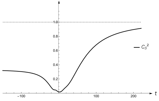
Figure 3: The sound speed squared of the scalar perturbations is non-negative for all times and asymptotically tends to 1 in the infinite future. The parameters $u$, $w$, $\tau$, $\Lambda$, $\alpha$ and $f$ are the same as in Fig. 1.

Figure 4: The plots of $\Theta$, $(\mathcal{G_{T}}+\mathcal{D})$ and $\xi$ in our model; these functions play the crucial role in evading the no-go theorem.

The scalar sound speed squared is given in Fig. 3; it confirms the subluminal propagation of perturbations at early times and reveals that $c_{\mathcal{S}}^{2}|_{t\to+\infty}\to 1$, as expected for the massless scalar field, at late times. Let us recall that we have chosen $\mathcal{G_{T}}=\mathcal{F_{T}}=1$, and hence $c_{\mathcal{T}}^{2}=1$.

We plot the functions $\xi$, $(\mathcal{G_{T}}+\mathcal{D})$ and $\Theta$ in Fig. 4 to clarify the way we evade the no-go theorem with our solution and ensure that the inequality (9) holds.

Hence, the reconstructed beyond Horndeski Lagrangian is an explicit example of the theory admitting a complete, stable Genesis solution with both asymptotics described by GR. The solution is indeed free of instabilities of all kinds and does not suffer from superluminal modes.

4 Conclusion

In this work, we have revisited the Genesis scenario in beyond Horndeski theory and suggested a modified version of it. We have constructed a specific Lagrangian of beyond Horndeski type, which admits the completely stable solution with the Genesis epoch at early times and both asymptotics described by GR as $t\to\pm\infty$. Unlike the previous version of the scenario suggested in Ref. [3], the dynamics during the Genesis stage is similar to that in the original Genesis model of Ref. [2] and is driven by the cubic Galileon, while at late times the theory tends to GR + a conventional massless scalar field. The novel feature is the simple behaviour of the theory in both the asymptotic past and future, which results from allowing $\gamma$-crossing in our model. We have strengthened the point raised in Refs. [3, 27] that $\gamma$-crossing is the key to constructing ever-stable non-singular solutions with both asymptotics described by GR. The stability of the Genesis solution as well as the required form of asymptotics are explicitly established and follow from the reconstruction procedure. Our judicial choice of the Lagrangian also ensured safe subluminal or at most luminal propagation of both scalar and tensor modes at all times. It is worth noting that in our model, tensor modes propagate at the speed of light, which is safe from the observational viewpoint. Moreover, since long enough after the Genesis epoch the theory reduces to that of a conventional massless scalar field and GR, the late-time cosmological behavior is the standard hot stage (provided, of course, that the energy density of our scalar is converted into heat), so no constraints on our Lagrangian functions emerge. The suggested Genesis solution with the ascribed set of properties is a promising candidate for describing the early time evolution within the realistic cosmological models.

5 Acknowledgements

The work has been supported by Russian Science Foundation Grant No. 19-12-00393.

References

- [1] P. Creminelli, A. Nicolis and E. Trincherini, “Galilean Genesis: An Alternative to inflation,” JCAP 1011 (2010) 021 [arXiv:1007.0027 [hep-th]]
- [2] P. Creminelli, K. Hinterbichler, J. Khoury, A. Nicolis and E. Trincherini, “Subluminal Galilean Genesis,” JHEP 1302 (2013) 006 [arXiv:1209.3768 [hep-th]].
- [3] R. Kolevatov, S. Mironov, N. Sukhov and V. Volkova, “Cosmological bounce and Genesis beyond Horndeski,” JCAP 1708 (2017) no.08, 038 [arXiv:1705.06626 [hep-th]].
- [4] V. A. Rubakov, “The Null Energy Condition and its violation,” Phys. Usp. 57 (2014) 128 [Usp. Fiz. Nauk 184 (2014) no.2, 137] [arXiv:1401.4024 [hep-th]].
- [5] F. J. Tipler, “Energy conditions and spacetime singularities,” Phys. Rev. D 17 (1978) 2521.
- [6] G. W. Horndeski, “Second-order scalar-tensor field equations in a four-dimensional space,” Int. J. Theor. Phys. 10, 363 (1974).
- [7] C. Deffayet, X. Gao, D. A. Steer and G. Zahariade, “From k-essence to generalised Galileons,” Phys. Rev. D 84 (2011) 064039 [arXiv:1103.3260 [hep-th]].
- [8] M. Zumalacárregui and J. García-Bellido, “Transforming gravity: from derivative couplings to matter to second-order scalar-tensor theories beyond the Horndeski Lagrangian,” Phys. Rev. D 89 (2014) 064046 [arXiv:1308.4685 [gr-qc]].
- [9] J. Gleyzes, D. Langlois, F. Piazza and F. Vernizzi, “Healthy theories beyond Horndeski,” Phys. Rev. Lett. 114 (2015) no.21, 211101 [arXiv:1404.6495 [hep-th]].
- [10] D. Langlois and K. Noui, “Degenerate higher derivative theories beyond Horndeski: evading the Ostrogradski instability,” JCAP 1602 (2016) no.02, 034 [arXiv:1510.06930 [gr-qc]].
- [11] J. Ben Achour, M. Crisostomi, K. Koyama, D. Langlois, K. Noui and G. Tasinato, “Degenerate higher order scalar-tensor theories beyond Horndeski up to cubic order,” JHEP 1612 (2016) 100 [arXiv:1608.08135 [hep-th]].
- [12] D. Langlois, M. Mancarella, K. Noui and F. Vernizzi, “Effective Description of Higher-Order Scalar-Tensor Theories,” JCAP 1705 (2017) no.05, 033, [arXiv:1703.03797 [hep-th]].
- [13] D. Langlois, “Dark Energy and Modified Gravity in Degenerate Higher-Order Scalar-Tensor (DHOST) theories: a review,” Int. J. Mod. Phys. D 28 (2019) no.05, 1942006 [arXiv:1811.06271 [gr-qc]].
- [14] T. Kobayashi, “Horndeski theory and beyond: a review,” Rept. Prog. Phys. 82 (2019) no.8, 086901 [arXiv:1901.07183 [gr-qc]].
- [15] K. Hinterbichler, A. Joyce, J. Khoury and G. E. J. Miller, “Dirac-Born-Infeld Genesis: An Improved Violation of the Null Energy Condition,” Phys. Rev. Lett. 110 (2013) no.24, 241303 [arXiv:1212.3607 [hep-th]].
- [16] S. Nishi, T. Kobayashi, N. Tanahashi and M. Yamaguchi, “Cosmological matching conditionsand galilean genesis in Horndeski’s theory,” JCAP 1403 (2014) 008 [arXiv:1401.1045 [hep-th]].
- [17] S. Nishi and T. Kobayashi, “Scale-invariant perturbations from null-energy-condition violation: A new variant of Galilean genesis,” Phys. Rev. D 95 (2017) no.6, 064001 [arXiv:1611.01906 [hep-th]].
- [18] M. Libanov, S. Mironov and V. Rubakov, “Generalized Galileons: instabilities of bouncing and Genesis cosmologies and modified Genesis,” JCAP 1608 (2016) no.08, 037 [arXiv:1605.05992 [hep-th]].
- [19] T. Kobayashi, “Generic instabilities of nonsingular cosmologies in Horndeski theory: A no-go theorem,” Phys. Rev. D 94 (2016) no.4, 043511 [arXiv:1606.05831 [hep-th]].
- [20] A. Ijjas and P. J. Steinhardt, “Classically stable nonsingular cosmological bounces,” Phys. Rev. Lett. 117 (2016) no.12, 121304 doi:10.1103/PhysRevLett.117.121304 [arXiv:1606.08880 [gr-qc]].
- [21] Y. A. Ageeva, O. A. Evseev, O. I. Melichev and V. A. Rubakov, “Horndeski Genesis: strong coupling and absence thereof,” [arXiv:1810.00465 [hep-th]].
- [22] R. Kolevatov and S. Mironov, “Cosmological bounces and Lorentzian wormholes in Galileon theories with an extra scalar field,” Phys. Rev. D 94 (2016) no.12, 123516 [arXiv:1607.04099 [hep-th]].
- [23] S. Akama and T. Kobayashi, “Generalized multi-Galileons, covariantized new terms, and the no-go theorem for nonsingular cosmologies,” Phys. Rev. D 95 (2017) no.6, 064011 [arXiv:1701.02926 [hep-th]].
- [24] Y. Cai, Y. Wan, H. G. Li, T. Qiu and Y. S. Piao, “The Effective Field Theory of nonsingular cosmology,” JHEP 1701 (2017) 090 [arXiv:1610.03400 [gr-qc]].
- [25] P. Creminelli, D. Pirtskhalava, L. Santoni and E. Trincherini, “Stability of Geodesically Complete Cosmologies,” JCAP 1611 (2016) no.11, 047 [arXiv:1610.04207 [hep-th]].
- [26] Y. Cai and Y. S. Piao, “A covariant Lagrangian for stable nonsingular bounce,” JHEP 1709 (2017) 027 [arXiv:1705.03401 [gr-qc]].
- [27] S. Mironov, V. Rubakov and V. Volkova, “Bounce beyond Horndeski with GR asymptotics and -crossing,” JCAP 1810 (2018) no.10, 050 [arXiv:1807.08361 [hep-th]].
- [28] A. Ijjas, “Space-time slicing in Horndeski theories and its implications for non-singular bouncing solutions,” JCAP 1802 (2018) no.02, 007 [arXiv:1710.05990 [gr-qc]].
- [29] T. Kobayashi, M. Yamaguchi and J. Yokoyama, “Generalized G-inflation: Inflation with the most general second-order field equations,” Prog. Theor. Phys. 126 (2011) 511 [arXiv:1105.5723 [hep-th]].
- [30] R. Kolevatov, S. Mironov, V. Rubakov, N. Sukhov and V. Volkova, “Cosmological bounce in Horndeski theory and beyond,” EPJ Web Conf. 191 (2018) 07013.
- [31] S. Mironov, “Mathematical Formulation of the No-Go Theorem in Horndeski Theory,” Universe 5 (2019) no.2, 52.