Budget-Aware Adapters for Multi-Domain Learning

Abstract

Multi-Domain Learning (MDL) refers to the problem of learning a set of models derived from a common deep architecture, each one specialized to perform a task in a certain domain (e.g., photos, sketches, paintings). This paper tackles MDL with a particular interest in obtaining domain-specific models with an adjustable budget in terms of the number of network parameters and computational complexity. Our intuition is that, as in real applications the number of domains and tasks can be very large, an effective MDL approach should not only focus on accuracy but also on having as few parameters as possible. To implement this idea we derive specialized deep models for each domain by adapting a pre-trained architecture but, differently from other methods, we propose a novel strategy to automatically adjust the computational complexity of the network. To this aim, we introduce Budget-Aware Adapters that select the most relevant feature channels to better handle data from a novel domain. Some constraints on the number of active switches are imposed in order to obtain a network respecting the desired complexity budget. Experimentally, we show that our approach leads to recognition accuracy competitive with state-of-the-art approaches but with much lighter networks both in terms of storage and computation.

1 Introduction

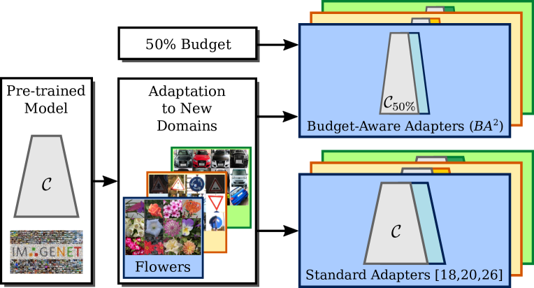
Figure 1: In Multi-Domain Learning, a pre-trained model is usually adapted to solve new tasks in new domains. When using standard approaches, the complexity $\mathcal{C}$ of the domain-specific models is dependent on the pre-trained model complexity. In this work we propose a novel approach to learn specialized models while imposing budget constraints in terms of the number of parameters for each new domain.

Deep learning methods have brought revolutionary advances in computer vision, setting the state of the art in many tasks such as object recognition [9, 14], detection [7], semantic segmentation [4], depth estimation [37], and many more. Despite these progresses, a major drawback with deep architectures is that when a novel task is addressed typically a new model is required. However, in many situations it may be reasonable to learn models which perform well on data from different domains. This problem, referred as Multi-Domain Learning (MDL) and originally proposed in [25], has received considerable attention lately [18, 20, 26]. An example of MDL is the problem of image classification when the data belong to several domains (e.g., natural images, paintings, sketches, etc.) and the categories in the different domains do not overlap.

Previous MDL approaches [18, 20, 25, 26] utilize a common backbone architecture (i.e., a pre-trained model) and learn a limited set of domain-specific parameters. This strategy is advantageous with respect to building several independent classifiers, as it guarantees a significant saving in terms of memory. Furthermore, it naturally deals with the catastrophic forgetting issue, as when a new domain is considered the knowledge on the previously learned ones is retained. Existing approaches mostly differ from the way domain-specific parameters are designed and integrated within the backbone architecture. For instance, binary masks are employed in [18, 20] in order to select the parameters of the main network that are useful for a given task. Differently, in [25, 26] domain-specific residual blocks are embedded in the original deep architecture. While the different approaches are typically compared in terms of classification accuracy, their computational and memory requirements are not taken into account.

In this paper we argue that an optimal MDL algorithm should not only achieve high recognition accuracy on all the different domains but should also permit to keep the number of parameters as low as possible. In fact, as in real world applications the number of domains and tasks can be very large, it is desirable to limit the models’ complexity (both in terms of memory and computation). Furthermore, it is very reasonable to assume that different domains and tasks may correspond to a different degree of difficulty (e.g., recognizing digits is usually easier than classifying flowers) and may require different models: small networks should be used for easy tasks, while models with a large number of parameters should be employed for difficult ones.

Following these ideas, we propose the first MDL approach which derives a set of domain-specific classifiers from a common backbone deep architecture under a budget constraint, where the budget is specified by a user and is expressed as the number of network parameters (see Figure 1). This idea is realized by designing a new network module, called Budget-Aware Adapters (BA²), which embeds switch variables that can select the feature channels relevant to a domain. By dropping feature channels in each convolutional layer, BA² both adapt the image representation of the network and reduce the computational complexity. Furthermore, we propose a constrained optimization problem formulation in order to train domain-specific classifiers that respect budget constraints provided by the user. The proposed approach has been evaluated on two publicly available benchmarks, the ten datasets of the Visual Decathlon Challenge [25] and the six-dataset benchmark proposed in [18]. Our results show that the proposed method is competitive with state-of-the-art baselines and requires much less storage and computational resources.

2 Related Work

Multi-domain Learning. The problem of adapting deep architectures to novel tasks and domains has been extensively studied in the past. Earlier works considered simple strategies, such as fine-tuning existing pre-trained models, with the drawback of incurring to catastrophic forgetting and of requiring the storage of multiple specialized models. More recent studies address the problem proposing methods for extending the capabilities of existing deep architectures by adding few task-specific parameters. In this way, as the parameters of the original network are left untouched, the catastrophic forgetting issue is naturally circumvented. For instance, Rebuffi et al. [25] introduced residual adapters, i.e., a novel design for residual blocks that embed task-specific components. In a subsequent work [26], they proposed an improved architecture where the topology of the adapters is parallel rather than series. Rosenfeld et al. [27] employed controller modules to constrain newly learned parameters to be linear combinations of existing ones. Weight-based pruning has been considered in [19] to adapt a single neural network to multiple tasks. Aiming at decreasing the overhead in terms of storage, more recent works proposed to adopt binary masks [18, 20] as task-specific parameters. In particular, while in [18] simple multiplicative binary masks are used to indicate which parameters are and which are not useful for a new task, [20] proposes a more general formulation considering affine transformations. Guo et al. [8] proposed an adaptive fine-tuning method and derive specialized classifiers by fine-tuning certain layers according to a given target image.

While these works considered a supervised learning setting, the idea of learning task-specific parameters has also been considered in reinforcement learning. For instance Rusu et al. [29] proposed an approach where each novel task is addressed by adding a side branch to the main network. While our approach also aims at developing architectures which adapts a pretrained model to novel tasks, we target for the first time the problem of automatically adjusting the complexity of the task-specific models.

Incremental and Life-long learning. In the last few years several works have addressed the problem of incremental [2, 24] and life-long learning [1, 11, 16], considering different strategies to avoid catastrophic forgetting. For instance, Li and Hoeim [16] proposed to adopt knowledge distillation to ensure that the model adapted to the new tasks is also effective for the old ones. Kirkpatrick et al. [11] demonstrated that a good strategy to avoid forgetting on the old tasks is to selectively slow down learning on the weights important for those tasks. In [1] Aljundi et al. presented Memory Aware Synapses, where the idea is to estimate the importance weights for the network parameters in an unsupervised manner in order to allow adaptation to unlabeled data stream. However, while these works are interested in learning over multiple tasks in sequence, in this paper we focus on a different problem, i.e., re-configuring an existing architecture under some resource constraints.

Adaptive and Resource-aware Networks. The problem of designing deep architectures which allow an adaptive accuracy-efficiency trade-off directly at runtime has been recently addressed in the research community. For instance, Wu et al. [36] proposed BlockDrop, an approach that learns to dynamically choose which layers of a Residual Network to drop at test time to reduce the computational cost while retaining the prediction accuracy. Wang et al. [34] introduced novel gating functions to automatically define at test time the computational graph based on the current network input. Slimmable Networks have been introduced in [38] with the purpose of adjusting the network width according to resource constraints. While our approach is inspired by these methods, in this paper we show that the idea of dynamically adjusting the network according to resource constraints is especially beneficial in the multi-domain setting.

3 Budget-Aware Adapters for MDL

In Multi-Domain Learning (MDL), the goal is to learn a single model that can work for diverse visual domains, such as pictures from the web, medical images, paintings, etc. Importantly, when the visual domains are very different, the model has to adapt its image representation. To address MDL, we follow the common approach [18, 25] that consists in learning Convolutional Neural Networks (ConvNets) that share the vast majority of their parameters but employ a very limited number of additional parameters specifically trained for each domain.

Formally, we consider an arbitrary pre-trained ConvNet $\Psi_{0}(\cdot;\theta_{0}):\mathcal{X}\to\mathcal{Y}_{0}$ with parameters $\theta_{0}$ that assigns class labels in ${\cal Y}_{0}$ to elements of an input space $\cal X$ (e.g., images). Our goal is to learn for each domain $d\in\{1,\ldots,D\}$, a classifier $\Psi_{d}(\cdot;\theta_{0},\theta_{a}^{d}):\mathcal{X}\to\mathcal{Y}_{d}$ with a possibly different output space ${\cal Y}_{d}$ that shares the vast majority of its parameters $\theta_{0}$ but exploits additional domain-specific parameters $\theta_{a}^{d}$ to adapt $\Psi_{d}$ to the domain $d$.

In this paper, we claim that an effective approach for MDL should require a low number of domain-specific parameters. In other words, the cardinality of each $\theta_{a}^{d}$ parameter set should be negligible with respect to the cardinality of $\theta_{0}$. In addition, we argue that one major drawback of previous MDL methods is that the network computational complexity directly ensues from the initial pre-trained network $\Psi_{0}$. More precisely, the networks $\Psi_{d}$ for the new domains usually have computational complexities at best equal to the one of the initial pre-trained network. Moreover, such models lack flexibility for deployment since the user cannot adjust the computational complexity of $\Psi_{d}$ depending on its needs or on hardware constraints.

To address this issue, we introduce novel modules, the Budget-Aware Adapters (BA²) that are designed both for enabling a pre-trained model to handle a new domain and for controlling the network complexity. The key idea behind BA² is that the parameters $\theta_{a}^{d}$ control the use of the convolution operations parametrized by $\theta_{0}$. Therefore, BA² can learn to drop parts of the computational graph of $\Psi_{0}$ and parts of the parameters $\theta_{0}$ resulting in a model $\Psi_{d}$ with a lower computational complexity and fewer parameters to load at inference time. In the following, we first describe the proposed Budget-Aware Adapters (Subsection 3.1) and then present the training procedure we introduced to learn domain-specific models with budget constraints (Subsection 3.2).

3.1 Adapting Convolutions with BA²

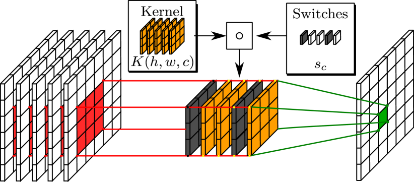
Figure 2: Budget-Aware Adapters (BA²): a switch vector controls the activation of convolution channels in order to both adapt the network to a new domain and adjust its computational complexity. Dark grey arrays represents channels that are “turned off” by the switches.

We now describe our Budget-Aware Adapters illustrated in Figure 2. Since, BA² acts on the elementary convolution operation, it can be employed in any ConvNet but, for the sake of notation simplicity, we consider the case of 2D convolutions. Let $\boldsymbol{K}\in\mathbb{R}^{2K_{H}+1\times 2K_{W}+1\times C}$ be a kernel of a standard convolutional layer of $\Psi_{0}$. Here $2K_{H}+1$ and $2K_{W}+1$ denote the kernel size and $C$ the number of input channels. Note that $\boldsymbol{K}$ is a subset of the parameters $\theta_{0}$ introduced in Section 3. Considering a standard 2D convolution, an input feature map $\boldsymbol{I}\in\mathbb{R}^{H\times W\times C}$ and an activation function $g$, the output value at the location $(i,j)\in[1..H]\times[1..W]$ is given by:

$$\boldsymbol{x}(i,j)=g\Big{(}\sum_{c=1}^{C}\phi_{c}(i,j)\Big{)},$$ (1)

where $\phi_{c}$ is given by:

$$\phi_{c}=\sum_{h=-K_{h}}^{K_{h}}\sum_{w=-K_{w}}^{K_{w}}\boldsymbol{K}(h,w,c)\boldsymbol{I}(i-h,j-w,c).$$ (2)

For the sake of simplicity, the kernel parameter tensor $\boldsymbol{K}$ is indexed from $-K_{h}$ to $K_{h}$ and from $-K_{w}$ to $K_{w}$. When learning a new domain $d$, we propose to adapt the convolution by controlling the use of each channel of the convolution layer. To this aim, we introduce an additional binary switch vector $s\in\{0,1\}^{C}$. This vector $s$ is a subset of the $\theta_{a}^{d}$ introduced in Section 3. As shown in Figure 3.1, each switch value is used for an entire channel. As a consequence, BA² results in a limited number of additional parameters. Formally, the output of the adapted convolution at location $(i,j)$ is given by:

$$\boldsymbol{x}(i,j)=g\Big{(}\sum_{c=1}^{C}s_{c}\phi_{c}(i,j)\Big{)}$$ (3)

Note that, when $s_{c}=0$, the tensor $\phi_{c}$ in Equation (3) does not need to be computed. In this context, by adjusting the proportion of zeros in $s_{c}$, we can control the computational complexity of the convolution layer. Furthermore, in Equation (2), when $\phi_{c}$ is not computed, the kernel weights values $\boldsymbol{K}(h,w,c)$ can be removed from the computational graph and do not need to be stored. Therefore, in scenarios where the parameters $\boldsymbol{K}$ of the initial networks are not further used, these $\boldsymbol{K}(h,w,c)$ weights can be dropped resulting in a lower number of parameters to store. Thus, $s_{c}$ can also control the number of parameters of the new domain networks.

In order to obtain a model that can be trained via Stochastic Gradient Descent, we follow [10, 18] and obtain binary values using a threshold function $\tau$:

$$s_{c}=\tau(\tilde{s}_{c})=\left\{\begin{array}[]{ll}0&\tilde{s}_{c}\leq 0.0\\ 1&\text{otherwise}\end{array}\right.$$ (4)

where $\tilde{s}_{c}\in\mathbb{R}$ are continuous scalar parameters. Similarly to [10, 18], during backward propagation, the $\tau$ function is replaced by the identity function to be able to back-propagate the error and update $\tilde{s}_{c}$. Even though we learn $\tilde{s}_{c}$ at training time, we only need to store the binary $s_{c}$ values to use at testing time, leading to a small storage requirement (1-bit per $s_{c}$). Compared to other multi-domain methods that generally use additional 32-bit floating-point numbers [25, 26, 27], BA² results in a much lighter storage.

The proposed BA² have four main features:

Adapting image representation: In BA², the $\phi_{c}$ features can be interpreted as a filter bank and the switch vectors can be understood as a filter selector. Depending on the domain, different switch values can be employed to select features relevant for the considered domain.

Low computational complexity: After training, all the tensors $\{\phi_{c}\mid s_{c}=0\}$ can be removed of the computational graph, resulting in a lower computational complexity. More precisely, the computational complexity is proportional to:

$$\mathcal{C}=\frac{1}{C}\sum_{c=1}^{C}s_{c}.$$ (5)

Note that, the uncomputed operations are grouped in channels allowing fast GPU implementation.

Lower storage: First, the number of additional parameters is rather small compared to the number of kernel parameters of the base network. Second, at testing time, the additional switch parameters can be stored with a binary representation to obtain a lightweight storage (1-bit per kernel channel). Finally, the weight values $\{\boldsymbol{K}(h,w,c)\mid s_{c}=0\}$ can be dropped, obtaining models with fewer parameters for the new domains. Again, the number of parameters is proportional to $\mathcal{C}$ in Equation (5).

Low Memory footprint: Reducing the computational complexity, does not necessarily reduces the memory footprint at testing time. In order to properly reduce the memory footprint, one needs to reduce the memory requirements of all operations across the computational graph, as stated in [31]. Given that BA² works on the level of the convolution operation, it can also control the memory footprint.

Method	Params	ImNet	Airc.	C100	DPed	DTD	GTSR	Flwr.	Oglt.	SVHN	UCF	Mean	$S$-Score
Feature [25]	1	59.7	23.3	63.1	80.3	45.4	68.2	73.7	58.8	43.5	26.8	54.3	544
Finetune [25]	10	59.9	60.3	82.1	92.8	55.5	97.5	81.4	87.7	96.6	51.2	76.5	2500
SpotTune [8]	11	60.3	63.9	80.5	96.5	57.13	99.5	85.22	88.8	96.7	52.3	78.1	3612
RA[25]	2	59.7	56.7	81.2	93.9	50.9	97.1	66.2	89.6	96.1	47.5	73.9	2118
DAM [27]	2.17	57.7	64.1	80.1	91.3	56.5	98.5	86.1	89.7	96.8	49.4	77.0	2851
PA [26]	2	60.3	64.2	81.9	94.7	58.8	99.4	84.7	89.2	96.5	50.9	78.1	3412
PB [18]	1.28	57.7	65.3	79.9	97.0	57.5	97.3	79.1	87.6	97.2	47.5	76.6	2838
WTPB [20]	1.29	60.8	52.8	82.0	96.2	58.7	99.2	88.2	89.2	96.8	48.6	77.2	3497
BA2 (Ours) ($\beta=1.00$)	1.03	56.9	49.9	78.1	95.5	55.1	99.4	86.1	88.7	96.9	50.2	75.7	3199
BA2 (Ours) ($\beta=0.75$)	1.03	56.9	47.0	78.4	95.3	55.0	99.2	85.6	88.8	96.8	48.7	75.2	3063
BA2 (Ours) ($\beta=0.50$)	1.03	56.9	45.7	76.6	95.0	55.2	99.4	83.3	88.9	96.9	46.8	74.5	2999
BA2 (Ours) ($\beta=0.25$)	1.03	56.9	42.2	71.0	93.4	52.4	99.1	82.0	88.5	96.9	43.9	72.6	2538

Table 1: Results in terms of accuracy and $S$-Score, for the Visual Decathlon Challenge. Best model in bold, second best underlined.

3.2 Training Budget-aware adapters for MDL

We now detail how BA² is used for MDL. As explained in Subsection 3.1, we follow a strategy of adapting a pre-trained model to novel domains. Therefore, when learning a new domain, we consider that $\theta_{0}$ is provided and we keep it fixed for the whole training procedure.As a consequence the learning procedure can be subdivided in independent training for each domain resulting in simpler training procedure. Note that, similarly to [18, 20, 25], we use batch-normalization parameters specific for each domain. Furthermore, as shown in [38], using different number of channels leads to different feature mean and variance and, as a consequence, sharing Batch Normalization layers performs poorly. Therefore, we use different batch-normalization layers for each budget. Note that, since the number of parameters in a batch-normalization layer is much lower than in convolution layer, this solution does not increase significantly the number of additional parameters with respect to the size of $\theta_{0}$.

Following the notations introduced in Section 3, $\theta_{a}^{d}$ now denotes the set of all the switch values $s_{c}$ and the additional batch-normalization parameters. Considering a new domain $d$, $\Psi_{d}$ is trained using a loss $\mathcal{L}$. In the case of classification, we employ the cross-entropy loss for all the domains. In the context of BA², we aim at training $\Psi_{d}$ with budget constraints. Formally, we formulate the optimization problem as follows: we minimize $\mathcal{L}$ with respect to the BA² parameters $\theta_{a}^{d}$ such that the network complexity satisfies a target budget $\beta\in[0,1]$. For each new domain, we obtain the following constrained optimization problem:

$$\theta_{a}^{d*}= \operatorname*{\arg\min}_{\theta_{a}^{d}}\mathcal{L}(\theta_{0},\theta_{a}^{d})$$ (6)

$$s.t.~{}\bar{\theta_{a}^{d}}\leq\beta$$ (7)

where $\bar{\theta_{a}^{d}}$ denotes the mean value of the switches in $\theta_{a}^{d}$. From Equation (6), we construct the generalized Lagrange function and the associated optimization problem:

$$\theta_{a}^{d*}= \operatorname*{\arg\min}_{\theta_{a}^{d}}\big{[}\mathcal{L}(\theta_{0},\theta_{a}^{d})+\max_{\lambda\geq 0}(\lambda(\bar{\theta_{a}^{d}}-\beta))\big{]}.$$ (8)

The $\lambda$ is known as the Karush-Kuhn-Tucker (KKT) multiplier. Equation (8) is optimized via stochastic gradient descent (SGD). When the budget constrained is respected, $\lambda=0$ and Equation (8) corresponds to $\mathcal{L}$ minimization. When the constraint is not satisfied, in addition to $\mathcal{L}$ minimization, the SGD steps also lead to an increase of $\lambda$ which in turn increases the impact of the budget constraint on $\mathcal{L}$.

In order to obtained networks with different budgets, training is performed independently for each $\beta$ value. When $\beta$ is set to 1, the constraint in Equation (6) is satisfied for any $\theta_{a}^{d}$. Therefore, the problem consists in a loss minimization problem over the parametric network family defined by $\theta_{0}$. This scenario corresponds to a standard multi-domain scenario without considering budget as in [18, 20, 25, 27]. When $\beta<1$, we combine both re-parametrization and budget-adjustable abilities of Budget-Aware Adapters. In this case, the goal is to obtain the best performing model that respects the budget constrain. It is important to note that the actual complexity of the network, after training, can be lower than the one defined by the user, including the $\beta=1$ case.

Note that in Equation (6), the budget constraint is formulated as a constraint on the total network complexity. In practice, it can be preferable to constrain each BA² to satisfy independent budget constraints in order to both spread computation over the layers and obtain a lower memory footprint. In this case, KKT multipliers are added in Equation (8) for each convolution layer.

4 Experimental Results

In this section we present the experimental methodology and metrics used to evaluate our approach. Moreover, we report the results and comparisons with state of the art MDL approaches (Subsection 4.1). In addition, we also conduct further experiments on the usual single-domain setting and demonstrate the effectiveness of BA² (Subsection 4.3) in reducing complexity while learning accurate recognition models.

4.1 Multi-Domain Learning

Datasets.

In order to evaluate our MDL approach, we adopt two different benchmarks. We first consider the Visual Decathlon Challenge [25]. The purpose of this challenge is to compare methods for MDL over 10 different classification tasks: ImageNet [28], CIFAR-100 [13], Aircraft [17], Daimler pedestrian (DPed) [21], Describable Textures (DTD) [5], German Traffic Signs (GTSR) [33], Omniglot [15], SVHN [22], UCF101 Dynamic Images [3, 32] and VGG-Flowers [23]. For more details about the challenge, please refer to [25].

As for the second benchmark, we follow previous works [18, 20] and consider the union of six different datasets: ImageNet [28], VGG-Flowers [23], Stanford Cars [12], Caltech-UCSD Birds (CUBS) [35], Sketches [6], and WikiArt [30]. These datasets are very heterogeneous, comprising a wide range of the categories (e.g., cars [12] vs birds [35]) and a large variety of image appearance (i.e., natural images [28], art paintings [30], sketches [6]).

Accuracy Metrics. Both benchmarks are designed to address classification problems. Therefore, as common practice [18, 20], we report the accuracy for each domain and the average accuracy over the domains. In addition, the score function $S$, as introduced in [25], is considered to jointly account for the $N$ domains. The test error $E_{d}$ of the model on the domain $d$ is compared to the test error of a baseline model $E_{d}^{\text{max}}$. The score is given by $S=\sum^{N}_{d=1}\alpha\max\{0,E_{d}^{\textrm{max}}-E_{d}\}^{2}$, where $\alpha$ is a scaling parameter ensuring that the perfect score for each domain is 1000. The baseline error is given by doubling the error of 10 independent models fine-tuned for each domain. Importantly, this metric favors models with good performances over all domains, while penalizing those that are accurate only on few domains.

Complexity Metrics. Furthermore, since in this paper we argue that MDL methods should also be evaluated in terms of model complexity, we consider two other metrics which account for the number of network parameters and operations. First, following [18, 20], we report the total number of parameters relative to the ones of the initial pre-trained model (counting all domains and excluding the classifiers). Note that, when computing the model size, we consider that all float numbers are encoded in 32 bits and switches in 1 bit only. Second, we propose to report the average number of floating-point operations (FLOP) over all the domains (including the pre-training domain $d=0$, i.e., ImageNet) relative to the number of operations of the initial pre-trained network. Interestingly, for the Budget-Aware Adapters, this ratio is also equal to the average number of parameters used at inference time for each individual domain, relative to the number of parameters of $\Psi_{0}$.

These complexity measures lead us to two variants of the score $S$: the score per parameter $S_{P}$ and the score per operation $S_{O}$. These two metrics are able to assess the trade-off between performance and model complexity.

Networks and training protocols. Concerning the Visual Decathlon, we consider the Wide ResNet-28 [39] adopted in previous works [18, 20, 25, 27] and employ the same data pre-processing protocol. In term of hyper-parameters, we follow [25] when pre-training on ImageNet. For other domains, we employ the hyper-parameters used in [18].

For the second benchmark, we use a ResNet-50 [9]. Note that, since the performance of the method in [19] relies on the order of the domains, we report the performances for two orderings as in [18]: starting from the model pre-trained on ImageNet, the first ($\rightarrow$) corresponds to CUBS-Cars-Flowers-WikiArt-Sketch, while the second ($\leftarrow$) corresponds to reversed order. We also followed the pre-processing, hyper-parameters and training schedule of [18], as we did in the Visual Decathlon Challenge.

We chose to use the same setting (network, pre-processing, and training schedules) employed by previous works seeking fairer analyses regarding the impact of the proposed approach.

Budget Constraints Even if our training procedure is formulated as a constrained optimization problem (see Equation 7), the stochastic gradient descent algorithm we employ does not guarantee that all the constraints will be satisfied at the end of training. Therefore, in all our experiments, we check whether the final models respect the specified budget constraints. All the scores reported in this paper were obtained with models that respect the specified budget constraints, unless explicitly specified otherwise.

Method	FLOP	Params	Score	$S_{O}$	$S_{P}$
Feature	1	1	544	544	544
Finetune	1	10	2500	2500	250
SpotTune	1	11	3612	3612	328
RA	1.099	2	2118	1926	1059
DAM	1	2.17	2851	2851	1314
PA	1.099	2	3412	3102	1706
PB	1	1.28	2838	2838	2217
WTPB	1	1.29	3497	3497	2710
BA2 (Ours) ($\beta=1.00$)	0.646	1.03	3199	4952	3106
BA2 (Ours) ($\beta=0.75$)	0.612	1.03	3063	5005	2974
BA2 (Ours) ($\beta=0.50$)	0.543	1.03	2999	5523	2912
BA2 (Ours) ($\beta=0.25$)	0.325	1.03	2538	7809	2464

Table 2: Performance/Complexity trade-off comparison on the visual decathlon challenge.

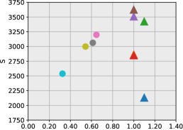
(a)

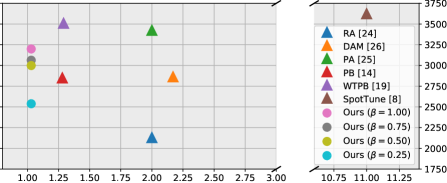
(b)

Figure 3: Performance/Complexity Trade-Off on the visual decathlon challenge: the total score is displayed as a function of the two considered complexity metrics FLOPs and Params.

	FLOP	Params	ImageNet	CUBS	Cars	Flowers	WikiArt	Sketch	Score	$S_{O}$	$S_{P}$
Classifier Only [18]	1	1	76.2	70.7	52.8	86.0	55.6	50.9	533	533	533
Individual Networks [18]	1	6	76.2	82.8	91.8	96.6	75.6	80.8	1500	1500	250
SpotTune [8]	1	7	76.2	84.03	92.40	96.34	75.77	80.2	1526	1526	218
PackNet $\rightarrow$ [19]	1	1.10	75.7	80.4	86.1	93.0	69.4	76.2	732	732	665
PackNet $\leftarrow$ [19]	1	1.10	75.7	71.4	80.0	90.6	70.3	78.7	620	620	534
Piggyback [18]	1	1.16	76.2	80.4	88.1	93.5	73.4	79.4	934	934	805
Piggyback+BN [18]	1	1.17	76.2	82.1	90.6	95.2	74.1	79.4	1184	1184	1012
WTPB [20]	1	1.17	76.2	82.6	91.5	96.5	74.8	80.2	1430	1430	1222
BA2 (Ours) ($\beta=1.00$)	0.700	1.03	76.2	81.19	92.14	95.74	72.32	79.28	1265	1807	1228
BA2 (Ours) ($\beta=0.75$)	0.600	1.03	76.2	79.44	90.62	94.44	70.92	79.38	1006	1677	977
BA2 (Ours) ($\beta=0.50$)	0.559	1.03	76.2	79.34	90.80	94.91	70.61	78.28	1012	1810	983
BA2 (Ours) ($\beta=0.25$)	0.375	1.03	76.2	78.01	88.15	93.19	67.99	77.85	755	2013	733

Table 3: State of the art comparison on the ImageNet-to-Sketch benchmark. Best model in bold, second best underlined.

Results on the Visual Decathlon Challenge. We first evaluate our methods on the Visual Decathlon Challenge. Results are reported in Table 1. We report the BA² scores with respect to four different budgets $\beta\in\{0.25,0.50,0.75,1.00\}$. We first observe that for most of the domains, BA² without budget constrains is competitive with state-of-the-art methods in terms of accuracy. Our method is the second best performing for three domains (GTSR, VGG-Flowers, and SVHN). In terms of score, among lightweight methods, only Parallel Adapters (PA) and Weight Transformations using Binary Masks (WTPB) perform better than ours. However, both methods require significantly more additional parameters to achieve these performances. Concerning the models where a budget constraint is considered, we observe that the scores still outperform RA [25], DAM [27] and PB [18] in terms of score when targeting a budget of 50% or 75% of the initial network parameters, i.e., $\beta=0.50\textrm{ or }0.75$.

Interestingly, it can be seen in Table 1 that, when we impose a tighter budget to BA², the total number of parameters do not decrease. Indeed, all the parameters of the pre-trained network $\Psi_{0}$ are still required at testing time to handle the 10 domains. Only the number of parameters used for each domain and the number of floating-point operations are reduced. Therefore, we propose to complete this evaluation in order to further understand the performance/complexity trade-off achieved by each method. More precisely, we report the number of parameters and FLOPs in Table 2, and their corresponding scores. First, we observe that only BA² models report FLOPs lower than 1. In other words, only BA² provide models with fewer operations than the initial network $\Psi_{0}$. We see that BA² achieve the best performance in terms of $S_{P}$ when using 100% budget. As mentioned above, the total number of parameters for the 10 domains do not decrease with a smaller budget. Consequently, smaller budgets obtain lower $S_{P}$ values. Nevertheless, the 75% and 50% models rank second and third, respectively.

Concerning the FLOP, only BA² return models with fewer floating-point operations than the initial network. As a consequence, BA² clearly outperforms other approaches in terms of $S_{O}$. In addition, we note that $S_{O}$ increases when using tighter budgets. It illustrates the potential of our approach in order to obtain a good performance/complexity trade-off. Interestingly, even the models with $\beta=100\%$ report a FLOP value lower than 1 since convolutional channels can be dropped to adapt to each domain. Note that for all our models, the reported FLOP numbers are smaller than the specified budget. The reason for this is that we impose budget constraints independently to each convolutional layer in order to obtain a low memory footprint (see Subsection 3.2). Therefore, the average percentage of channels that are dropped can be smaller than the specified budget and, in fact, this is what we observed in ours models.

For better visualization, we illustrate in Figure 3 the performance/complexity trade-off for each method on the Visual Decathlon Challenge. More precisely, in Figure 3a, we plot the score obtained as a function of the computation complexity in FLOPs. When comparing with other methods, we see that BA² lead to much lighter models that have, as a consequence, better performance/computation trade-offs. In Figure 3b, we report the obtained score as a function of the total number of parameters. BA² is the method that requires the lowest number of additional parameters to adapt to the 10 domains. Furthermore, this plot clearly show that our 100% model has an interesting trade-off between the performance and the number of additional parameters. Note that WTPB [20] also obtained a good trade-off but stores, in total, 29% more parameters (approximately $\times 9$ per new domain). Interestingly, the best performing approach in terms of score, i.e., SpotTune [8], requires a much larger number of parameters that would restrict the use of this method when increasing the number of domains.

Results on the ImageNet-to-Sketch setting. We now compare our method with state-of-the-art approaches on the ImageNet-to-Sketch setting. Results are reported in Table 3. First, we see that BA² achieve the second best score among methods that employ only a small number of additional parameters. Only WTPB [20] reports better scores at a higher cost in terms of additional parameters per domain. Interestingly, the 50% and 75% models report similar performances. Second, the $S_{O}$ and $S_{P}$ values clearly confirm the conclusions drawn on the first experiments on the Visual Decathlon Challenge. The four different BA² models outperform all the other methods in terms of $S_{O}$ and our model with 100% budget slightly outperforms WTPB in terms of $S_{P}$.

4.2 Ablation study of BA²

In order to further understand the performance of BA², we propose to compare the drop in accuracy when imposing different budget constraints. In Figure 4, we perform an experiment on the Visual Decathlon Challenge with varying budgets $\beta=\{0.1,0.2,\ldots,1.0\}$. We display the accuracy drop relative to the performance of the model with 100% budget. Because of the restrictions of the Challenge in terms of number of submissions (per day and in total), we report results on the validation set. To decrease the impact of the training stochasticity, we report the median performance over 4 runs. As mentioned previously, the stochastic gradient descent algorithm we employ for training our model does not guarantee to provide a solution that respect the budget constraints. Therefore, in Figure 4, we display only points corresponding to models that satisfy the specified budget. We first observe that for all the domains, our method returns models that respect the specified budget when the budget is greater than $30\%$. For some domains, we obtain models that respect even tighter budgets, such as the GTSR dataset where we obtain a 10%-budget model.

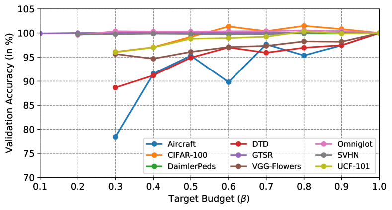
Figure 4: Relative accuracy drop compared to the 100% model accuracy for the 10 domains of the Visual Decathlon challenge datset (validation set). Median score over 4 runs is reported. Missing points correspond to models where the budget constraint was not satisfied in the four runs.

Interestingly, we notice that the domains where our models fail to respect the $20\%$ budget are the same in which the drop in performance is more clearly visible from the $100\%$ to $30\%$ budgets. Furthermore, we observe that the domains where the performance drop is small correspond to those where the $100\%$ model reaches excellent performance. For instance, in Table 1 the models for the GTSR (traffic signs) and DPed (pedestrians) datasets reach accuracy over $95\%$ with our $100\%$ model and do not significantly lose performance when imposing a tighter budget. Conversely, we observe that the DTD and the aircraft datasets, that show the largest performance drop, correspond also to the most challenging datasets according the accuracies of all methods reported in Table 1.

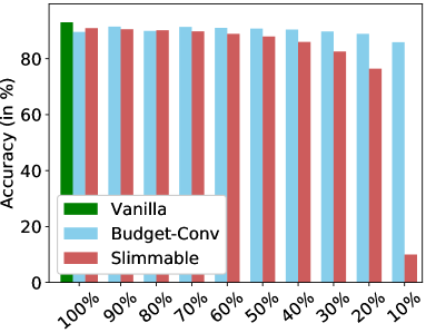
(a)

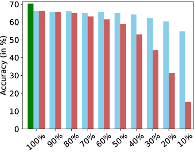
(b)

Figure 5: Single-domain classification with adaptive budget. BA² is compared with Slimmable Networks [38].

4.3 Evaluating BA² for single-domain problems

In order to further demonstrate the effectiveness of our proposed BA², we perform experiments on a standard single-domain classification problem training a single ConvNet with different budget constraints.

Datasets and Experimental Protocol. We perform experiments on two well-known classification datasets: CIFAR-10 and CIFAR-100 [13]. In these experiments, we employ the following procedure. We first train a ResNet-50 architecture setting all the switch vectors to 1, leading to the initial model. We then employ different switches $\theta_{s}$ for each budget, but we share the convolution parameters $\theta_{k}$ among budgets. We fine-tune all the parameters optimizing Equation (8) w.r.t. $\theta_{k}$ and all the different $\theta_{s}$ parameters jointly.

Results. We compare our approach with the recently proposed Slimmable Networks [38]. We consider this approach as this is the most closely related to our method in literature. In [38], different budgets are obtained by gradually dropping filters, imposing that filters dropped for a given budget are also dropped for lower budgets. Conversely, in BA² we do not impose any constraints between the switches at different budgets. It can be observed in Figure 5 that, in the case of CIFAR-10, both models achieve an accuracy similar to a vanilla network trained without any budget constraint. On the more challenging CIFAR-100, both BA² and Slimmable Networks perform slightly worse than the vanilla network. Interestingly, BA² is able to maintain a constant accuracy on both datasets when decreasing the budget constraint up to 50% whereas Slimmable Networks begins to perform poorly. The difference between the two methods becomes larger with tighter budgets, until 10% where Slimmable Networks accuracy collapses. These experiments show that imposing constraints between budgets as in [38] harms the performance and illustrate the potential of our approach even for single-domain problems.

5 Conclusions

In this paper, we proposed to investigate the multi-domain learning problem with budget constraints. We propose to adapt a pre-trained network to each new domain with constraints on the network complexity. Our Budget-Aware Adapters (BA²) select the most relevant feature channels using trainable switch vectors. We impose constraints on the switches to obtain networks that respect to user-specified budget constraints. From an experimental point of view, BA² show performances competitive with state-of-the-art methods even with small budget values. As future works, we plan to extend our Budget-Aware Adapters in order to be able do control the budget in a continuous fashion.

Acknowledgements

This work was carried out under the “Vision and Learning joint Laboratory” between FBK and UNITN, and financed in part by the Coordenação de Aperfeiçoamento de Pessoal de Nível Superior – Brasil (CAPES) – Finance Code 001; CNPq, Brasil (311504/2017-5); and FAPES, Brasil (455/2019).

Appendix

Here, we first provide more details about the training and evaluation protocols used in our experiments (Appendix A). Then, in Appendix B, we report additional experiments on the ImageNet-to-Sketch benchmark.

Appendix A Additional training and testing details

In order to draw a fair comparison with other methods, we employed the same training schedule and hyperparameters of previous works. Here, we provide more details about the training and test procedures used in the three experiments: (i) Visual Decathlon Challenge, (ii) ImageNet-to-Sketch benchmark, and (iii) Single-Domain Classification.

Visual Decathlon challenge

Following previous works [18, 20, 25, 27], we employ the Wide ResNet WRN-28-4-B(3,3), i.e., 28 convolutional layers with widening factor of 4 and the original “basic” block (2 convolutions using $3\times 3$ kernel size). As in [25, 20], random crops of $64\times 64$ pixels are used to feed the network during training. The optimizer parameters are set following [18, 20], where SGD with momentum is employed for the classifier and Adam for the rest of the architecture with initial learning rates of 0.001 and 0.0001, respectively. The model is trained with batch size of 32 for 60 epochs; after 45 epochs, the learning rates are decayed by a factor of 10. The real-valued switches ($\tilde{s}_{c}$) are initialized with a value of 0.001. In addition to random cropping, in regards to training data augmentation, horizontal mirroring is also applied with a 50% probability, except for four datasets (DTD, Omniglot, SVHN, and GTSR) on which it could be either harmful or useless. During training, the models for all the domains are initialized using the ImageNet pre-trained weights and these weights are kept fixed, i.e., only the domain-specific parameters ($\tilde{s}_{c}$, Batch Normalization and classifiers) are learned. At test time, we follow the procedure proposed in [14] and used in [20]. We employ a ten-crop strategy for the datasets in which horizontal mirroring was applied and five-crop otherwise. In the five-crop strategy, a crop is performed on each corner of the image in addition to a central one; the ten-crop adds horizontally mirrored versions of each one of the five crops. The final prediction is based on the average of the predictions over all the crops.

ImageNet-to-Sketch benchmark

We use the ResNet-50 as in [18, 20] feeding a random crop of $224\times 224$ pixels after resizing the images to $256\times 256$ pixels. In addition to random cropping, horizontal mirroring is applied to all datasets during training. The networks are initially trained using the same schedule as in [18, 20], i.e., 30 epochs with a learning rate drop (with a factor of 10) after 15 epochs. For the lowest budget ($\beta=0.25$), we add another learning rate drop at 30 epochs and train for additional 15 epochs in order to fully satisfy the constraints. All the other steps are performed as in the Visual Decathlon Challenge.

Single-domain classification

In these experiments, we use the same variant of the ResNet proposed in the original Residual Networks [9] paper for the CIFAR-10 dataset with $n=9$, which results in a ResNet with 56 layers. First, we train the baseline model, which is the model without switches. Since we are interested in single-domain learning for this experiment, we do not need to freeze the weights as in the multi-domain experiments. Therefore, we jointly train the switches and the weights using the baseline pre-trained weights as initialization. In these cases, we use SGD with momentum (initial learning rate of $0.1$) for both the baseline model and the joint training. Concerning data augmentation, we use random crops of $32\times 32$ pixels with 4 pixel padding and horizontal mirroring with 50% probability. The same setting is used for the CIFAR-100.

Appendix B Results

	FLOP	Params	ImageNet	CUBS	Cars	Flowers	WikiArt	Sketch	Score	$S_{O}$	$S_{P}$
Classifier Only [18]	1	1	74.4	73.5	56.8	83.4	54.9	53.1	328	328	328
Individual Networks [18]	1	6	74.4	81.7	91.4	96.5	76.4	80.5	1500	1500	250
PackNet $\rightarrow$ [19]	1	1.11	74.4	80.7	84.7	91.1	66.3	74.7	691	691	623
PackNet $\leftarrow$ [19]	1	1.11	74.4	69.6	77.9	91.5	69.2	78.9	610	610	550
Piggyback [18]	1	1.15	74.4	79.7	87.2	94.3	72.0	80.0	951	951	827
Piggyback+BN [18]	1	1.21	74.4	81.4	90.1	95.5	73.9	79.1	1215	1215	1004
WTPB [20]	1	1.21	74.4	81.7	91.6	96.9	75.7	79.8	1540	1540	1268
BA2 (Ours) ($\beta=1.00$)	0.687	1.17	74.4	82.4	92.9	96.0	71.5	79.9	1440	2096	1230
BA2 (Ours) ($\beta=0.75$)	0.578	1.17	74.4	81.2	91.9	94.9	68.9	79.9	1193	2064	1019
BA2 (Ours) ($\beta=0.50$)	0.543	1.17	74.4	78.2	89.2	95.0	66.2	78.8	925	1703	790
BA2 (Ours) ($\beta=0.25$)	0.375	1.17	74.4	76.2*	88.4*	94.7*	67.9*	78.4	840	2240	717

Table B.1: State-of-the-art comparison on the ImageNet-to-Sketch benchmark using DenseNet-121 architecture. (*) Even though the average sparsities are greater than 75%, these models did not satisfy the constraint for every single layer.

ImageNet-to-Sketch

In the paper, we report the results on the ImageNet-to-Sketch benchmark using the ResNet-50 architecture. In addition to this model, results using the DenseNet-121 are also reported in several works [18, 19, 20]. For that reason, we also provide these results in Table B.1. First, we see that our method achieves the best scores in two domains and the second best in three other domains. Interestingly, in the Cars domain, our method with $\beta=0.75$ is the second best model (only after our method with $\beta=1.00$), achieving results better than all the other methods using only 57.8% of the FLOP, on average. Concerning the number parameters, our approach is the second best in terms of Params. Indeed the number of batch normalization and $1\times 1$ convolutions parameters in the DenseNet-121 model with respect to the total number of parameters is higher than in the ResNet-50 model. Nevertheless, BA² is still the only one with FLOP less than 1. Finally, it can be noted that our method with $\beta=1.00$ still achieves a good trade-off between performance and complexity.

References

- [1] Rahaf Aljundi, Francesca Babiloni, Mohamed Elhoseiny, Marcus Rohrbach, and Tinne Tuytelaars. Memory Aware Synapses: Learning what (not) to forget. In European Conference on Computer Vision (ECCV), 2018.
- [2] Abhijit Bendale and Terrance E. Boult. Towards Open Set Deep Networks. In Conference on Computer Vision and Pattern Recognition (CVPR), 2016.
- [3] Hakan Bilen, Basura Fernando, Efstratios Gavves, Andrea Vedaldi, and Stephen Gould. Dynamic Image Networks for Action Recognition. In Conference on Computer Vision and Pattern Recognition (CVPR), 2016.
- [4] Liang-Chieh Chen, George Papandreou, Iasonas Kokkinos, Kevin Murphy, and Alan L Yuille. DeepLab: Semantic Image Segmentation with Deep Convolutional Nets, Atrous Convolution, and Fully Connected CRFs. IEEE Transactions on Pattern Analysis and Machine Intelligence, 40(4):834–848, 2018.
- [5] Mircea Cimpoi, Subhransu Maji, Iasonas Kokkinos, Sammy Mohamed, and Andrea Vedaldi. Describing Textures in the Wild. In Conference on Computer Vision and Pattern Recognition (CVPR), 2014.
- [6] Mathias Eitz, James Hays, and Marc Alexa. How Do Humans Sketch Objects? ACM Transactions on Graphics, 31(4):44:1–44:10, 2012.
- [7] Ross Girshick, Jeff Donahue, Trevor Darrell, and Jitendra Malik. Rich feature hierarchies for accurate object detection and semantic segmentation. In Conference on Computer Vision and Pattern Recognition (CVPR), 2014.
- [8] Yunhui Guo, Honghui Shi, Abhishek Kumar, Kristen Grauman, Tajana Rosing, and Rogerio Feris. SpotTune: Transfer Learning through Adaptive Fine-tuning. In Conference on Computer Vision and Pattern Recognition (CVPR), 2019.
- [9] Kaiming He, Xiangyu Zhang, Shaoqing Ren, and Jian Sun. Deep Residual Learning for Image Recognition. In Conference on Computer Vision and Pattern Recognition (CVPR), 2016.
- [10] Łukasz Kaiser, Aurko Roy, Ashish Vaswani, Niki Parmar, Samy Bengio, Jakob Uszkoreit, and Noam Shazeer. Fast Decoding in Sequence Models Using Discrete Latent Variables. In International Conference on Machine Learning (ICML), 2018.
- [11] James Kirkpatrick, Razvan Pascanu, Neil Rabinowitz, Joel Veness, Guillaume Desjardins, Andrei A Rusu, Kieran Milan, John Quan, Tiago Ramalho, Agnieszka Grabska-Barwinska, et al. Overcoming catastrophic forgetting in neural networks. Proceedings of the National Academy of Sciences, 114(13):3521–3526, 2017.
- [12] Jonathan Krause, Michael Stark, Jia Deng, and Li Fei-Fei. 3D Object Representations for Fine-Grained Categorization. In International Conference on Computer Vision Workshops (ICCVW), 2013.
- [13] Alex Krizhevsky. Learning multiple layers of features from tiny images. Master’s thesis, University of Toronto, 2009.
- [14] Alex Krizhevsky, Ilya Sutskever, and Geoffrey E. Hinton. ImageNet Classification with Deep Convolutional Neural Networks. In Advances in Neural Information Processing Systems (NeurIPS), 2012.
- [15] Brenden M. Lake, Ruslan Salakhutdinov, and Joshua B. Tenenbaum. Human-level concept learning through probabilistic program induction. Science, 350(6266):1332–1338, 2015.
- [16] Zhizhong Li and Derek Hoiem. Learning without Forgetting. IEEE Transactions on Pattern Analysis and Machine Intelligence, 40(12):2935–2947, 2017.
- [17] Subhransu Maji, Esa Rahtu, Juho Kannala, Matthew Blaschko, and Andrea Vedaldi. Fine-Grained Visual Classification of Aircraft. arXiv preprint arXiv:1306.5151, 2013.
- [18] Arun Mallya, Dillon Davis, and Svetlana Lazebnik. Piggyback: Adapting a Single Network to Multiple Tasks by Learning to Mask Weights. In European Conference on Computer Vision (ECCV), 2018.
- [19] Arun Mallya and Svetlana Lazebnik. PackNet: Adding Multiple Tasks to a Single Network by Iterative Pruning. In Conference on Computer Vision and Pattern Recognition (CVPR), 2018.
- [20] Massimiliano Mancini, Elisa Ricci, Barbara Caputo, and Samuel Rota Bulò. Adding New Tasks to a Single Network with Weight Transformations using Binary Masks. In European Conference on Computer Vision Workshops (ECCVW), 2018.
- [21] Stefan Munder and Dariu M. Gavrila. An Experimental Study on Pedestrian Classification. IEEE Transactions on Pattern Analysis and Machine Intelligence, 28(11):1863–1868, 2006.
- [22] Yuval Netzer, Tao Wang, Adam Coates, Alessandro Bissacco, Bo Wu, and Andrew Y. Ng. Reading Digits in Natural Images with Unsupervised Feature Learning. In NeurIPS Workshop on Deep Learning and Unsupervised Feature Learning, 2011.
- [23] Maria-Elena Nilsback and Andrew Zisserman. Automated Flower Classification over a Large Number of Classes. In Indian Conference on Computer Vision, Graphics & Image Processing, 2008.
- [24] Sylvestre-Alvise Rebuffi, Alexander Kolesnikov, Georg Sperl, and Christoph H. Lampert. iCaRL: Incremental Classifier and Representation Learning. In Conference on Computer Vision and Pattern Recognition (CVPR), 2017.
- [25] Sylvestre-Alvise Rebuffi, Hakan Bilen, and Andrea Vedaldi. Learning multiple visual domains with residual adapters. In Advances in Neural Information Processing Systems (NeurIPS), 2017.
- [26] Sylvestre-Alvise Rebuffi, Hakan Bilen, and Andrea Vedaldi. Efficient parametrization of multi-domain deep neural networks. In Conference on Computer Vision and Pattern Recognition (CVPR), 2018.
- [27] Amir Rosenfeld and John K. Tsotsos. Incremental Learning Through Deep Adaptation. IEEE Transactions on Pattern Analysis and Machine Intelligence, 2018. Early Access.
- [28] Olga Russakovsky, Jia Deng, Hao Su, Jonathan Krause, Sanjeev Satheesh, Sean Ma, Zhiheng Huang, Andrej Karpathy, Aditya Khosla, Michael Bernstein, et al. ImageNet Large Scale Visual Recognition Challenge. International Journal of Computer Vision, 115(3):211–252, 2015.
- [29] Andrei A. Rusu, Neil C. Rabinowitz, Guillaume Desjardins, Hubert Soyer, James Kirkpatrick, Koray Kavukcuoglu, Razvan Pascanu, and Raia Hadsell. Progressive Neural Networks. arXiv preprint arXiv:1606.04671, 2016.
- [30] Babak Saleh and Ahmed Elgammal. Large-scale Classification of Fine-Art Paintings: Learning The Right Metric on The Right Feature. International Journal for Digital Art History, 2016.
- [31] Mark Sandler, Andrew Howard, Menglong Zhu, Andrey Zhmoginov, and Liang-Chieh Chen. MobileNetV2: Inverted Residuals and Linear Bottlenecks. In Conference on Computer Vision and Pattern Recognition (CVPR), 2018.
- [32] Khurram Soomro, Amir Roshan Zamir, and Mubarak Shah. UCF101: A Dataset of 101 Human Actions Classes From Videos in The Wild. arXiv preprint arXiv:1212.0402, 2012.
- [33] Johannes Stallkamp, Marc Schlipsing, Jan Salmen, and Christian Igel. Man vs. computer: Benchmarking machine learning algorithms for traffic sign recognition. Neural Networks, 32:323–332, 2012.
- [34] Xin Wang, Fisher Yu, Zi-Yi Dou, Trevor Darrell, and Joseph E. Gonzalez. SkipNet: Learning Dynamic Routing in Convolutional Networks. In European Conference on Computer Vision (ECCV), 2018.
- [35] Peter Welinder, Steve Branson, Takeshi Mita, Catherine Wah, Florian Schroff, Serge Belongie, and Pietro Perona. Caltech-UCSD Birds 200. Technical Report CNS-TR-2010-001, California Institute of Technology, 2010.
- [36] Zuxuan Wu, Tushar Nagarajan, Abhishek Kumar, Steven Rennie, Larry S Davis, Kristen Grauman, and Rogerio Feris. BlockDrop: Dynamic Inference Paths in Residual Networks. In Conference on Computer Vision and Pattern Recognition (CVPR), 2018.
- [37] Dan Xu, Elisa Ricci, Wanli Ouyang, Xiaogang Wang, and Nicu Sebe. Multi-Scale Continuous CRFs as Sequential Deep Networks for Monocular Depth Estimation. In Conference on Computer Vision and Pattern Recognition (CVPR), 2017.
- [38] Jiahui Yu, Linjie Yang, Ning Xu, Jianchao Yang, and Thomas Huang. Slimmable Neural Networks. In International Conference on Learning Representations (ICLR), 2019.
- [39] Sergey Zagoruyko and Nikos Komodakis. Wide Residual Networks. In British Machine Vision Conference (BMVC), 2016.