Representing Schema Structure with Graph Neural Networks for Text-to-SQL Parsing
Abstract
Research on parsing language to SQL has largely ignored the structure of the database (DB) schema, either because the DB was very simple, or because it was observed at both training and test time. In Spider, a recently-released text-to-SQL dataset, new and complex DBs are given at test time, and so the structure of the DB schema can inform the predicted SQL query. In this paper, we present an encoder-decoder semantic parser, where the structure of the DB schema is encoded with a graph neural network, and this representation is later used at both encoding and decoding time. Evaluation shows that encoding the schema structure improves our parser accuracy from 33.8% to 39.4%, dramatically above the current state of the art, which is at 19.7%.
1 Introduction
Semantic parsing Zelle and Mooney (1996); Zettlemoyer and Collins (2005) has recently taken increased interest in parsing questions into SQL queries, due to the popularity of SQL as a query language for relational databases (DBs).
Work on parsing to SQL Zhong et al. (2017); Iyer et al. (2017); Finegan-Dollak et al. (2018); Yu et al. (2018a) has either involved simple DBs that contain just one table, or had a single DB that is observed at both training and test time. Consequently, modeling the schema structure received little attention. Recently, Yu et al. (2018b) presented Spider, a text-to-SQL dataset, where at test time questions are executed against unseen and complex DBs. In this zero-shot setup, an informative representation of the schema structure is important. Consider the questions in Figure 1: while their language structure is similar, in the first query a ‘join’ operation is necessary because the information is distributed across three tables, while in the other query no ‘join’ is needed.
In this work, we propose a semantic parser that strongly uses the schema structure. We represent the structure of the schema as a graph, and use graph neural networks (GNNs) to provide a global representation for each node Li et al. (2016); De Cao et al. (2019); Sorokin and Gurevych (2018). We incorporate our schema representation into the encoder-decoder parser of Krishnamurthy et al. (2017), which was designed to parse questions into queries against unseen semi-structured tables. At encoding time we enrich each question word with a representation of the subgraph it is related to, and at decoding time we emit symbols from the schema that are related through the graph to previously decoded symbols.
We evaluate our parser on Spider, and show that encoding the schema structure improves accuracy from 33.8% to 39.4% (and from 14.6% to 26.8% on questions that involve multiple tables), well beyond 19.7%, the current state-of-the-art. We make our code publicly available at https://github.com/benbogin/spider-schema-gnn.
Find the age of students who do not have a cat pet.
SELECT age FROM student WHERE
student NOT IN (SELECT ... FROM student JOIN has_pet ... JOIN pets ... WHERE ...)
What are the names of teams that do not have match season record?
SELECT name FROM team WHERE
team_id NOT IN (SELECT team FROM match_season)
2 Problem Setup
We are given a training set , where is a natural language question, is its translation to a SQL query, and is the schema of the DB where is executed. Our goal is to learn a function that maps an unseen question-schema pair to its correct SQL query. Importantly, the schema was not seen at training time, that is, for all .
A DB schema includes: (a) The set of DB tables (e.g., singer), (b) a set of columns for each (e.g., singer_name), and (c) a set of foreign key-primary key column pairs , where each is a relation from a foreign-key in one table to a primary-key in another. We term all schema tables and columns as schema items and denote them by .
3 A Neural Semantic Parser for SQL
We base our model on the parser of Krishnamurthy et al. (2017), along with a grammar for SQL provided by AllenNLP Gardner et al. (2018); Lin et al. (2019), which covers 98.3% of the examples in Spider. This parser uses a linking mechanism for handling unobserved DB constants at test time. We review this model in the context of text-to-SQL parsing, focusing on components we expand upon in §4.
Linking schema items
To handle unseen schema items, Krishnamurthy et al. (2017) learn a similarity score between a word and a schema item that has type .111Types are tables, string columns, number columns, etc. The score is based on learned word embeddings and a few manually-crafted features.
The linking score is used to compute
where are all schema items of type and for words that do not link to any schema item. The functions and will be used to decode unseen schema items.
Encoder
A Bidirectional LSTM Hochreiter and Schmidhuber (1997) provides a contextualized representation for each question word . Importantly, the encoder input at time step is : the concatenation of the word embedding for and , where is a learned embedding for the schema item , based on the type of and its schema neighbors. Thus, augments every word with information on the schema items it should link to.
Decoder
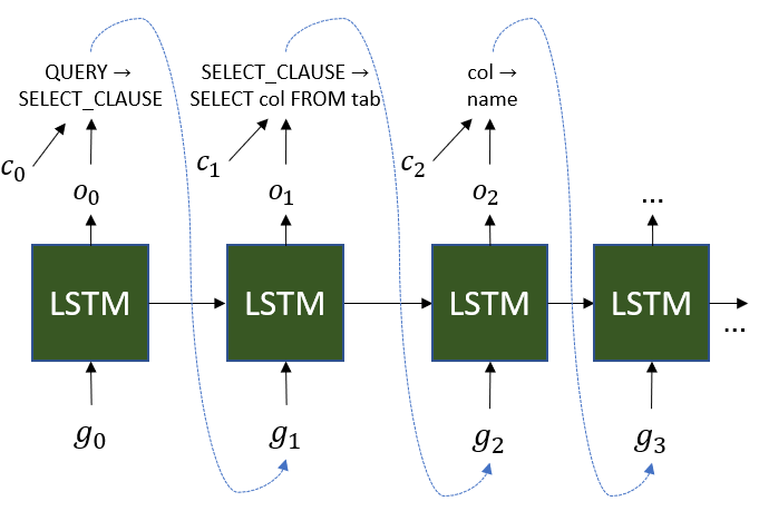
We use a grammar-based Xiao et al. (2016); Cheng et al. (2017); Yin and Neubig (2017); Rabinovich et al. (2017) LSTM decoder with attention on the input question (Figure 2). At each decoding step, a non-terminal of type is expanded using one of the grammar rules. Rules are either schema-independent and generate non-terminals or SQL keywords, or schema-specific and generate schema items.
At each decoding step , the decoding LSTM takes a vector as input, which is an embedding of the grammar rule decoded in the previous step, and outputs a vector . If this rule is schema-independent, is a learned global embedding. If it is schema-specific, i.e., a schema item was generated, is a learned embedding of its type. An attention distribution over the input words is computed in a standard manner Bahdanau et al. (2015), where the attention score for every word is . It is then used to compute the weighted average of the input . Now a distribution over grammar rules is computed by:
where , are the number of legal rules (according to the grammar) that can be chosen at time step for schema-independent and schema-specific rules respectively. The score is computed with a feed-forward network, and the score is computed for all legal schema items by multiplying the matrix , which contains the relevant linking scores , with the attention vector . Thus, decoding unseen schema items is done by first attending to the question words, which are linked to the schema items.
4 Modeling Schemas with GNNs
Schema structure is informative for predicting the SQL query. Consider a table with two columns, where each is a foreign key to two other tables (student_semester table in Figure 3). Such a table is commonly used for describing a many-to-many relation between two other tables, which affects the output query. We now show how we represent this information in a neural parser and use it to improve predictions.
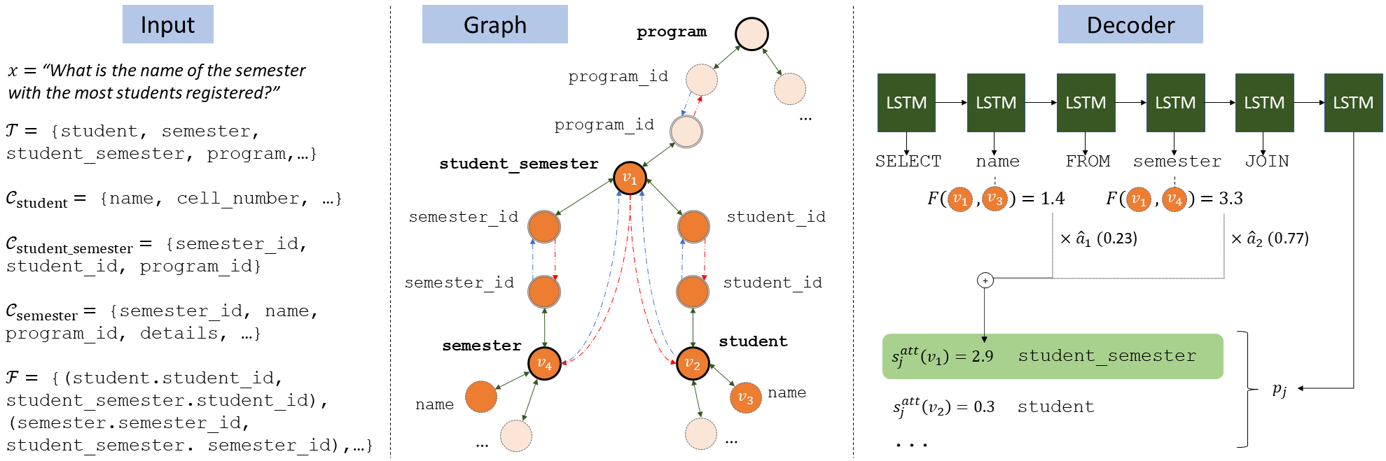
At a high-level our model has the following parts (Figure 3). (a) The schema is converted to a graph. (b) The graph is softly pruned conditioned on the input question. (c) A Graph neural network generates a representation for nodes that is aware of the global schema structure. (d) The encoder and decoder use the schema representation. We will now elaborate on each part.
Schema-to-graph
To convert the schema to a graph (Figure 3, left), we define the graph nodes as the schema items . We add three types of edges: for each column in a table , we add edges and to the edge set (green edges). For each foreign-primary key column pair , we add edges and to the edge set and edges and to (dashed edges). Edge types are used by the graph neural network to capture different ways in which columns and tables relate to one another.
Question-conditioned relevance
Each question refers to different parts of the schema, and thus, our representation should change conditioned on the question. For example, in Figure 3, the relation between the tables student_semester and program is irrelevant. To model that, we re-use the distribution from §3, and define a relevance score for a schema item : — the maximum probability of for any word . We use this score next to create a question-conditioned graph representation. Figure 3 shows relevant schema items in dark orange, and irrelevant items in light orange.
Neural graph representation
To learn a node representation that considers its relevance score and the global schema structure, we use gated GNNs Li et al. (2016). Each node is given an initial embedding conditioned on the relevance score: . We then apply the GNN recurrence for steps. At each step, each node re-computes its representation based on the representation of its neighbors in the previous step:
and then is computed as following, using a standard GRU Cho et al. (2014) update:
(see Li et al. (2016) for further details).
We denote the final representation of each schema item after steps by . We now show how this representation is used by the parser.
Encoder
In §3, a weighted average over schema items was concatenated to every word . To enjoy the schema-aware representations, we compute , which is identical to , except is used instead of . We concatenate to the output of the encoder , so that each word is augmented with the graph structure around the schema items it is linked to.
Decoder
As mentioned (§3), when a schema item is decoded, the input in the next time step is its type . A first change is to replace by , which has knowledge of the structure around . A second change is a self-attention mechanism that links to the schema, which we describe next.
When scoring a schema item, its score should depend on its relation to previously decoded schema items. E.g., in Figure 3, once the table semester has been decoded, it is likely to be joined to a related table. We capture this intuition with a self-attention mechanism.
For each decoding step , we denote by the hidden state of the decoder, and by the list of time steps before where a schema item has been decoded. We define the matrix , which concatenates the hidden states from all these time steps. We now compute a self-attention distribution over these time steps, and score schema items based on this distribution (Figure 3, right):
where the matrix computes a similarity between schema items that were previously decoded, and schema items that are legal according to the grammar: , where is a feed-forward network. Thus, the score of a schema item increases, if substantial attention is placed on schema items to which it bears high similarity.
Training
We maximize the log-likelihood of the gold sequence during training, and use beam-search (of size 10) at test time, similar to Krishnamurthy et al. 2017 and prior work. We run the GNN for steps.
5 Experiments and Results
Experimental setup
We evaluate on Spider Yu et al. (2018b), which contains 7,000/1,034/2,147 train/development/test examples.
We pre-process examples to remove table aliases (AS T1/T2/...) from the queries and use the explicit table name instead (i.e. we replace T1.col with table1_name.col), as in the majority of the cases ( 99% in Spider) these aliases are redundant. In addition, we add a table reference to all columns that do not have one (i.e. we replace col with table_name.col).
We use the official evaluation script from Spider to ≈compute accuracy, i.e., whether the predicted query is equivalent to the gold query.
Results
Our full model (GNN) obtains 39.4% accuracy on the test set, substantially higher than prior state-of-the-art (SyntaxSQLNet), which is at 19.7%. Removing the GNN from the parser (No GNN), which results in the parser of Krishnamurthy et al. (2017), augmented with a grammar for SQL, obtains an accuracy of 33.8%, showing the importance of encoding the schema structure.
| Model | Acc. | Single | Multi |
| SQLNet | 10.9% | 13.6% | 3.3% |
| SyntaxSQLNet | 18.9% | 23.1% | 7.0% |
| No GNN | 34.9% | 52.3% | 14.6% |
| GNN | 40.7% | 52.2% | 26.8% |
| - No Self Attend | 38.7% | 54.5% | 20.3% |
| - Only self attend | 35.9% | 47.1% | 23.0% |
| - No Rel. | 37.0% | 50.4% | 21.5% |
| GNN Oracle Rel. | 54.3% | 63.5% | 43.7% |
Table 1 shows results on the development set for baselines and ablations. The first column describes accuracy on the entire dataset, and the next two columns show accuracy when partitioning examples to queries involving only one table (Single) vs. more than one table (Multi).
GNN dramatically outperforms previously published baselines SQLNet and SyntaxSQLNet, and improves the performance of No GNN from 34.9% to 40.7%. Importantly, using schema structure specifically improves performance on questions with multiple tables from 14.6% to 26.8%.
We ablate the major novel components of our model to assess their impact. First, we remove the self-attention component (No Self Attend). We observe that performance drops by 2 points, where Single slightly improves, and Multi drops by 6.5 points. Second, to verify that improvement is not only due to self-attention, we ablate all other uses of the GNN. Namely, We use a model identical to No GNN, except it can access the GNN representations through the self-attention (Only Self Attend). We observe a large drop in performance to 35.9%, showing that all components are important. Last, we ablate the relevance score by setting for all schema items (No Rel.). Indeed, accuracy drops to 37.0%.
To assess the ceiling performance possible with a perfect relevance score, we run an oracle experiment, where we set for all schema items that are in the gold query, and for all other schema items (GNN Oracle Rel.). We see that a perfect relevance score substantially improves performance to 54.3%, indicating substantial headroom for future research.
join analysis For any model, we can examine the proportion of predicted queries with a join, where the structure of the join is “bad”: (a) when the join condition clause uses the same table twice (ON t1.column1 = t1.column2), and (b) when the joined table are not connected through a primary-foreign key relation.
We find that No GNN predicts such joins in 83.4% of the cases, while GNN does so in only 15.6% of cases. When automatically omitting from the beam candidates where condition (a) occurs, No GNN predicts a “bad” join in 14.2% of the cases vs. 4.3% for GNN (total accuracy increases by 0.3% for both models). As an example, in Figure 3, scores the table student the highest, although it is not related to the previously decoded table semester. Adding the self-attention score corrects this and leads to the correct student_semester, probably because the model learns to prefer connected tables.
6 Conclusion
We present a semantic parser that encodes the structure of the DB schema with a graph neural network, and uses this representation to make schema-aware decisions both at encoding and decoding time. We demonstrate the effectivness of this method on Spider, a dataset that contains complex schemas which are not seen at training time, and show substantial improvement over current state-of-the-art.
Acknowledgments
We thank Kevin Lin and Mark Neumann from Allen Institute for Artificial Intelligence for their help with the SQL grammar. This research was supported by Facebook. This work was completed in partial fulfillment for the Ph.D degree of the first author.
References
- Bahdanau et al. (2015) D. Bahdanau, K. Cho, and Y. Bengio. 2015. Neural machine translation by jointly learning to align and translate. In International Conference on Learning Representations (ICLR).
- Cheng et al. (2017) J. Cheng, S. Reddy, V. Saraswat, and M. Lapata. 2017. Learning structured natural language representations for semantic parsing. In Association for Computational Linguistics (ACL).
- Cho et al. (2014) K. Cho, B. van Merrienboer, C. Gulcehre, D. Bahdanau, F. Bougares, H. Schwenk, and Y. Bengio. 2014. Learning phrase representations using RNN encoder-decoder for statistical machine translation. In Empirical Methods in Natural Language Processing (EMNLP), pages 1724–1734.
- De Cao et al. (2019) N. De Cao, W. Aziz, and I. Titov. 2019. Question answering by reasoning across documents with graph convolutional networks. In North American Association for Computational Linguistics (NAACL).
- Finegan-Dollak et al. (2018) C. Finegan-Dollak, J. K. Kummerfeld, L. Zhang, K. Ramanathan, S. Sadasivam, R. Zhang, and D. Radev. 2018. Improving text-to-sql evaluation methodology. In Association for Computational Linguistics (ACL).
- Gardner et al. (2018) M. Gardner, J. Grus, M. Neumann, O. Tafjord, P. Dasigi, N. Liu, M. Peters, M. Schmitz, and L. Zettlemoyer. 2018. AllenNLP: A deep semantic natural language processing platform. arXiv preprint arXiv:1803.07640.
- Hochreiter and Schmidhuber (1997) S. Hochreiter and J. Schmidhuber. 1997. Long short-term memory. Neural Computation, 9(8):1735–1780.
- Iyer et al. (2017) S. Iyer, I. Konstas, A. Cheung, J. Krishnamurthy, and L. Zettlemoyer. 2017. Learning a neural semantic parser from user feedback. In Association for Computational Linguistics (ACL).
- Krishnamurthy et al. (2017) J. Krishnamurthy, P. Dasigi, and M. Gardner. 2017. Neural semantic parsing with type constraints for semi-structured tables. In Empirical Methods in Natural Language Processing (EMNLP).
- Li et al. (2016) Y. Li, D. Tarlow, M. Brockschmidt, and R. Zemel. 2016. Gated graph sequence neural networks. In International Conference on Learning Representations (ICLR).
- Lin et al. (2019) K. Lin, B. Bogin, M. Neumann, J. Berant, and M. Gardner. 2019. Grammar-based neural text-to-sql generation. arXiv preprint arXiv:1905.13326.
- Rabinovich et al. (2017) M. Rabinovich, M. Stern, and D. Klein. 2017. Abstract syntax networks for code generation and semantic parsing. In Association for Computational Linguistics (ACL).
- Sorokin and Gurevych (2018) D. Sorokin and I. Gurevych. 2018. Modeling semantics with gated graph neural networks for knowledge base question answering. In International Conference on Computational Linguistics (COLING).
- Xiao et al. (2016) C. Xiao, M. Dymetman, and C. Gardent. 2016. Sequence-based structured prediction for semantic parsing. In Association for Computational Linguistics (ACL).
- Yin and Neubig (2017) P. Yin and G. Neubig. 2017. A syntactic neural model for general-purpose code generation. In Association for Computational Linguistics (ACL), pages 440–450.
- Yu et al. (2018a) T. Yu, M. Yasunaga, K. Yang, R. Zhang, D. Wang, Z. Li, and D. Radev. 2018a. SyntaxSQLNet: Syntax tree networks for complex and cross-domaintext-to-SQL task. In Empirical Methods in Natural Language Processing (EMNLP).
- Yu et al. (2018b) T. Yu, R. Zhang, K. Yang, M. Yasunaga, D. Wang, Z. Li, J. Ma, I. Li, Q. Yao, S. Roman, Z. Zhang, and D. Radev. 2018b. Spider: A large-scale human-labeled dataset for complex and cross-domain semantic parsing and text-to-SQL task. In Empirical Methods in Natural Language Processing (EMNLP).
- Zelle and Mooney (1996) M. Zelle and R. J. Mooney. 1996. Learning to parse database queries using inductive logic programming. In Association for the Advancement of Artificial Intelligence (AAAI), pages 1050–1055.
- Zettlemoyer and Collins (2005) L. S. Zettlemoyer and M. Collins. 2005. Learning to map sentences to logical form: Structured classification with probabilistic categorial grammars. In Uncertainty in Artificial Intelligence (UAI), pages 658–666.
- Zhong et al. (2017) V. Zhong, C. Xiong, and R. Socher. 2017. Seq2sql: Generating structured queries from natural language using reinforcement learning. arXiv preprint arXiv:1709.00103.
| Question: List the names of poker players ordered by the final tables made in ascending order. |
|---|
| poker player: [’poker player id’, ’people id’, ’final table made’, ’best finish’, ’money rank’, ’earnings’] |
| people: [’people id’, ’nationality’, ’name’, ’birth date’, ’height’] |
|
GNN: SELECT people.name FROM poker_player JOIN people ON poker_player.people_id =
people.people_id ORDER BY poker_player.final_table_made ASC |
| NoGNN: SELECT people.name FROM people ORDER BY people.name DESC |
| Question: Which city has the most frequent destination airport? |
| airlines: [’airline id’, ’airline name’, ’abbreviation’, ’country’] |
| airports: [’city’, ’airport code’, ’airport name’, ’country’, ’country abbrev’] |
| flights: [’airline’, ’flight number’, ’source airport’, ’destination airport’] |
|
GNN: SELECT airports.city FROM airports JOIN flights ON airports.airportcode =
flights.destairport GROUP BY airports.city ORDER BY count (*) DESC LIMIT 1 |
|
NoGNN: SELECT airports.city FROM airports GROUP BY airports.city ORDER BY count (*)
DESC LIMIT 1 |
| Question: What are the names of airports in Aberdeen? |
| airlines: [’airline id’, ’airline name’, ’abbreviation’, ’country’] |
| airports: [’city’, ’airport code’, ’airport name’, ’country’, ’country abbrev’] |
| flights: [’airline’, ’flight number’, ’source airport’, ’destination airport’] |
|
GNN: SELECT airports.airportname FROM airports WHERE airports.airportname =
"value" |
| NoGNN: SELECT airports.airportname FROM airports WHERE airports.city = "value" |
| Question: List the language used least number of TV Channel. List language and number of TV Channel. |
| tv channel: [’id’, ’series name’, ’country’, ’language’, ’content’, ’pixel aspect ratio par’, ’hight definition tv’, ’pay per view ppv’, ’package option’] |
| tv series: [’id’, ’episode’, ’air date’, ’rating’, ’share’, ’18 49 rating share’, ’viewers m’, ’weekly rank’, ’channel’] |
| cartoon: [’id’, ’title’, ’directed by’, ’written by’, ’original air date’, ’production code’, ’channel’] |
|
GNN: SELECT tv_channel.language, count (*) FROM tv_channel GROUP BY
tv_channel.language ORDER BY count (*) ASC LIMIT 1 |
|
NoGNN: SELECT tv_channel.language, count (*) FROM tv_channel GROUP BY
tv_channel.language |
| Question: Find the type and weight of the youngest pet. |
| student: [’student id’, ’last name’, ’first name’, ’age’, ’sex’, ’major’, ’advisor’, ’city code’] |
| has pet: [’student id’, ’pet id’] |
| pets: [’pet id’, ’pet type’, ’pet age’, ’weight’] |
| GNN: SELECT pets.pettype, pets.weight FROM pets ORDER BY pets.pet_age LIMIT 1 |
| NoGNN: SELECT pets.pettype, pets.weight, pets.pet_age FROM pets |
| Question: List each owner’s first name, last name, and the size of his for her dog. |
| breeds: [’breed code’, ’breed name’] |
| charges: [’charge id’, ’charge type’, ’charge amount’] |
| sizes: [’size code’, ’size description’] |
| treatment types: [’treatment type code’, ’treatment type description’] |
| owners: [’owner id’, ’first name’, ’last name’, ’street’, ’city’, ’state’, ’zip code’, ’email address’, ’home phone’, ’cell number’] |
| dogs: [’dog id’, ’owner id’, ’abandoned yes or no’, ’breed code’, ’size code’, ’name’, ’age’, ’date of birth’, ’gender’, ’weight’, ’date arrived’, ’date adopted’, ’date departed’] |
| professionals: [’professional id’, ’role code’, ’first name’, ’street’, ’city’, ’state’, ’zip code’, ’last name’, ’email address’, ’home phone’, ’cell number’] |
| treatments: [’treatment id’, ’dog id’, ’professional id’, ’treatment type code’, ’date of treatment’, ’cost of treatment’] |
|
GNN: SELECT owners.first_name, owners.last_name, dogs.size_code FROM dogs JOIN
owners ON dogs.owner_id = owners.owner_id |
|
NoGNN: SELECT owners.first_name, owners.last_name, count (*) FROM dogs JOIN owners
ON dogs.owner_id = owners.owner_id GROUP BY owners.owner_id |
| Question: What is the number of carsw ith over 6 cylinders? |
| continents: [’cont id’, ’continent’] |
| countries: [’country id’, ’country name’, ’continent’] |
| car makers: [’id’, ’maker’, ’full name’, ’country’] |
| model list: [’model id’, ’maker’, ’model’] |
| car names: [’make id’, ’model’, ’make’] |
| cars data: [’id’, ’mpg’, ’cylinders’, ’edispl’, ’horsepower’, ’weight’, ’accelerate’, ’year’] |
| GNN: SELECT count (*) FROM cars_data WHERE cars_data.cylinders > "value" |
|
NoGNN: SELECT count (*) FROM model_list JOIN cars_data ON cars_data.id =
cars_data.id WHERE cars_data.cylinders > "value" |