Optimizing the Linear Fascicle Evaluation Algorithm for Multi-Core and Many-Core Systems

Abstract.

Sparse matrix-vector multiplication (SpMV) operations are commonly used in various scientific and engineering applications. The performance of the SpMV operation often depends on exploiting regularity patterns in the matrix. Various representations and optimization techniques have been proposed to minimize the memory bandwidth bottleneck arising from the irregular memory access pattern involved. Among recent representation techniques, tensor decomposition is a popular one used for very large but sparse matrices. Post sparse-tensor decomposition, the new representation involves indirect accesses, making it challenging to optimize for multi-cores and even more demanding for the massively parallel architectures, such as on GPUs.

Computational neuroscience algorithms often involve sparse datasets while still performing long-running computations on them. The Linear Fascicle Evaluation (LiFE) application is a popular neuroscience algorithm used for pruning brain connectivity graphs. The datasets employed herein involve the Sparse Tucker Decomposition (STD) — a widely used tensor decomposition method. Using this decomposition leads to multiple indirect array references, making it very difficult to optimize on both multi-core and many-core systems. Recent implementations of the LiFE algorithm show that its SpMV operations are the key bottleneck for performance and scaling. In this work, we first propose target-independent optimizations to optimize these SpMV operations, followed by target-dependent optimizations for CPU and GPU systems. The target-independent techniques include: (1) standard compiler optimizations to prevent unnecessary and redundant computations, (2) data restructuring techniques to minimize the effects of indirect accesses, and (3) methods to partition computations among threads to obtain coarse-grained parallelism with low synchronization overhead. Then we present the target-dependent optimizations for CPUs such as: (1) efficient synchronization-free thread mapping, and (2) utilizing BLAS calls to exploit hardware-specific speed. Following that, we present various GPU-specific optimizations to optimally map threads at the granularity of warps, thread blocks and grid. Furthermore, to automate the CPU-based optimizations developed for this algorithm, we also extend the PolyMage domain-specific language, embedded in Python. Our highly optimized and parallelized CPU implementation obtain a speedup of $6.3\times$ over the naive parallel CPU implementation running on 16-core Intel Xeon Silver (Skylake-based) system. In addition to that our optimized GPU implementation achieves a speedup of $5.2\times$ over a reference optimized GPU code version on NVIDIA’s GeForce RTX 2080 Ti GPU, and a speedup of $9.7\times$ over our highly optimized and parallelized CPU implementation.

1. Introduction

Sparse matrix-vector multiplication (SpMV) is a key operation in many scientific and engineering applications. As SpMV is typically memory bandwidth and latency bound, it plays a significant role in determining the overall execution time as well as the scalability of an application. Utilizing the architecture-specific memory model to reduce its memory bandwidth requirement is a major challenge, especially for highly parallel architectures such as GPUs, where exploiting the regularity in unstructured accesses is key. Numerous prior works have been proposed to improve the performance of SpMV, including that of the development of new sparse representations ⁵⁹; ¹³; ⁸⁸, representation-specific optimizations ¹³; ¹²; ³⁶ and architecture-specific techniques ⁹; ¹³; ⁵⁴; ⁶²; ⁹⁹; ¹⁰¹; ¹⁰³; ⁸¹.

Tensor decomposition ⁴⁷ is a popular technique to represent the LHS matrix in SpMV as a combination of a tensor and other auxiliary data structures in a way that drastically reduces the amount of storage. Tensor decomposition has found use to perform SpMV operations efficiently across many domains such as digital signal processing ²⁵; ⁸²; ⁴⁹; ⁵⁰; ⁵¹, machine learning ⁸², data mining ⁷²; ⁸⁶; ⁸⁷; ⁵; ⁶, computational biology ⁵³; ¹⁹; ⁶⁹; ⁶⁷; ⁶⁸; ³; ⁴; ⁹⁷; ⁶¹; ⁶⁵; ¹¹ and several more mentioned by Kolda and Bader ⁴⁷. Tucker et al. ⁹¹ presented a widely used tensor decomposition technique based on high-order singular value decomposition. Tucker’s technique is used in a range of applications ¹⁰⁶; ¹⁰⁵; ⁷⁴; ⁴⁷. More importantly, the Tucker model is used to perform low-rank decomposition of tensors to depict the sparse representations of matrices, and this is commonly referred to as the Sparse Tucker Decomposition (STD) ⁹¹. The major challenge for an STD-based application however is that the sparse representation entails multiple indirect array accesses. Therefore, efficiently utilizing multi-core and many-core architectures poses a significant difficulty because such accesses are both memory latency and bandwidth unfriendly. However, employing STD for an SpMV operation is a necessary trade-off considering the reduction in memory utilization obtained for a sparse matrix.

Building brain connectivity graphs or the wiring diagram of neural circuitry of the brain, termed as connectome, is an exciting computational neuroscience conundrum involving large but sparse matrices. Understanding the neural pathways is key to studying the connection between brain-regions and behavior. Principally, a connectome can be described at various scales based on the spatial resolution ⁸³; ¹⁰⁰; ⁶³. The scales can be primarily categorized as microscale, mesoscale and macroscale ⁴⁴. A microscale connectome is a neuron-to-neuron brain graph involving $10^{11}$ nodes (neurons) and $10^{17}$ edges (neuronal connection); currently, obtaining and processing such large data appears infeasible. A mesoscale connectome building technique is based on anatomical properties of the brain, which again is not a viable choice due to poor resolution of electron-microscopy ⁴¹; ¹⁶. Once technology is enhanced, optimizing such large sparse datasets will still be a formidable problem. In contrast, a macroscale level connectome ²⁸ divides a brain model into 3D volumes called voxels (in the order of $10^{6}$ in number); this is thus a much more tractable approach.

Diffusion-weighted Magnetic Resonance Imaging (dMRI) is a popular macroscale choice, that captures the diffusion of water molecules in the brain. The dMRI along with tractography techniques can be used to estimate white matter connectivity in the human brain. These pathways represent physical connections between brain regions and when analyzed in conjunction with behaviour, can provide interesting insights into brain-behaviour relationships. These insights are often essential in diagnosing diseases of the brain such as Alzheimer’s Disease ⁷⁰, a neurodegenerative disorder involving degradation of white matter. While the non-invasive nature of dMRI enables studying structural connectivity in-vivo in humans, it suffers from a major limitation in that the validity of the results cannot be tested easily due to the lack of access to ground truth ³⁹; ⁶⁰. Data acquisition protocols and tractography approaches often depend on the specific scientific questions being addressed and can differ significantly across cohorts. Thus, a standardized evaluation technique to assess connectomes and establish evidence for white matter pathways is critical for accurate and reliable estimation of structural connectivity in the brain.

One such technique that addresses these shortcomings is the Linear Fascicle Evaluation (LiFE) ⁷⁷; ¹⁸; ¹⁹, an algorithm that prunes white matter connectomes to produce an optimized subset of fibers that best explain the underlying diffusion signal. LiFE posits that the diffusion signal in a voxel (a volume of brain tissue) can be approximated by a weighted sum of the individual contribution of every streamline traversing that voxel. The model thus entails a simple constrained optimization problem where the weights associated with every streamline are estimated by minimizing the error between the measured and predicted diffusion signal. This optimization is carried out using a variant of the gradient descent method - the Subspace Barzilai-Borwein non-negative least squares (SBBNNLS) algorithm ⁴⁵, and involves iterative matrix multiplications. However, large execution times and memory requirements have precluded the large-scale use of the LiFE algorithm. While the memory issues have recently been addressed with the use of sparse representations (Sparse Tucker Decomposition ⁹¹) of the data, the matrix-vector multiplications, transformed to a more complex sequence of operations as presented by Pestilli and Caiafa ¹⁸ are still computationally demanding, involving multiple indirect array accesses. Optimizing the transformed SpMV operations on both multi-cores and GPUs is a challenging task that is memory latency and bandwidth bound even for low-resolution dMRI datasets.

In literature, several prior works have been proposed to tackle irregular applications for both multi-core and GPU systems such as ⁷; ⁵⁵; ⁸⁴; ⁹⁵; ⁹³; ⁹⁴. These approaches use inspector/executor paradigm ⁷ to exploit regularity in unstructured accesses. One such approach is presented by Venkat et al. ⁹⁵ to automate the code generation for a particular class of application performing SpMV on GPUs. Other studies show various compiler transformations to reduce the runtime overhead of code generation by the inspector step in ⁹³, and generate optimized code for wavefront parallelization for sparse-matrix representation in ⁹⁴. These works have presented a semi-automatic approach to analyze the data (using the inspector step) and then generate the optimized code (using the executor step). Note that these works are limited to read non-affine accesses. However, our work targets optimization of the SpMV operations of LiFE, where the sparse matrix is decomposed using the STD technique. The new representation of the matrix involves multiple irregular accesses which includes both read as well as write array access. Therefore, due to presence of such type of accesses, the exiting works will have a high runtime overhead. However, in this work, we present a specific data restructuring method tuned for LiFE with low run-time overhead. Furthermore, the prior works amortizes the overhead due to inspector/executor across the iterations of a loop in a program. In contrast, our work amortizes the overhead due to restructuring across the several runs of the same program along with the iterations of a loop. Additionally, our data restructuring optimization could potentially be generalized and extended to other applications employing STD, although one would have to look for similar or other data patterns. Thus, our work proposes a tailored data restructuring method to tackles indirect access of SpMV operations used in LiFE.

Prior works on optimizing the LiFE application considered distributed systems and GPUs. Gugnani et al. ³⁵ proposed a distributed memory based approach using MPI and OpenMP paradigms to parallelize the SpMV operations of LiFE and obtained a speedup of $8.7\times$ over the original approach. On the other hand, Madhav ⁵⁷ developed a fast GPU implementation to optimize the SpMV operations of LiFE by incorporating simple optimization techniques. In another work, Kumar et al. ⁴⁸ proposed a GPU-accelerated implementation for ReAl-LiFE ⁴⁸, a modification of LiFE application that introduced regularized pruning constraint to build connectomes.

In this work, we optimize the SpMV operations by performing a number of target-independent and target-dependent optimizations. The target optimizations comprises: (1) standard compiler optimizations, (2) various data restructuring methods, and (3) techniques to partition computations among threads. These optimizations can be automated and extended to other applications performing SpMV operations where the matrix is decomposed using STD. The target-dependent optimizations that we propose for multi-core architectures are following: (1) efficient synchronization-free thread mapping, and (2) utilizing BLAS calls, and for the GPUs the optimizations includes optimal techniques to map threads at the granularity of warps, thread blocks and grids. Tailoring these optimizations for the LiFE application, we obtain a speedup of $27.12\times$ for our highly optimized and parallelized CPU code over the original sequential implementation, and speedups of $5.2\times$ and $1.87\times$ for our optimized GPU implementation over a reference optimized GPU implementation (developed by Madhav ⁵⁷) and over the ReAl-LiFE GPU implementation (tweaked to perform same computations as the LiFE application) respectively. In addition, our work can express the SpMV operation of LiFE in a high-level language and abstract out other information using a domain-specific language (DSL) approach. Using the domain information, we can perform optimizations that provide significant improvements in performance and productivity. As a proof-of-concept, we extend PolyMage ⁷¹, a DSL designed for image processing pipelines, to express the key matrix operations in LiFE and automatically generate optimized CPU code to obtain similar performance improvements compared to that of our hand-optimized CPU implementation.

The key contributions of this paper are as follows:

• We address challenges involved in optimizing SpMV operations of the LiFE application on multi-cores and GPUs by proposing various architecture-agnostic and architecture-dependent optimizations.

• The target independent optimizations includes: (1) standard compiler optimizations to avoid unnecessary and redundant computations, (2) data restructuring methods to deal with multiple indirect array references that in turn make further optimizations valid and fruitful, and (3) effective partitioning of computations among threads to exploit coarse-grained parallelism while avoiding the usage of an atomic operation.

• The CPU-specific optimizations comprises: (1) efficient synchronization-free thread mapping method to reduce load imbalance, and (2) mapping to BLAS calls to exploit fine-grained parallelism.

• The GPU-specific optimizations include: (1) leveraging fine-grained parallelism by utilizing a GPU’s resources such as shared memory and the shuffle instruction, and (2) effectively transforming loops to map iterations in a better way.

• Then we present new constructs added to the PolyMage DSL to represent a sparse matrix and automatically generate optimized CPU code for the SpMV operations of the LiFE application.

• We present experimental results and analysis to show the usefulness of the optimizations we incorporated for SpMV of LiFE, and also compare them with the existing implementations.

• We present experimental results and analysis by varying various LiFE application parameters such as the number of voxels, number of fibers and different tractography techniques used to process the dMRI data for generating a connectome in the LiFE.

The rest of this paper is organized as follows. We provide background on the LiFE application in Section 2. We describe the problem and challenges pertaining to optimizing SpMV computations of LiFE in Section 3. The target-dependent and the target-independent optimizations are described in Section 4. Then we present the constructs developed in the PolyMage DSL to generate an optimized parallelized CPU code for the SpMV operations in Section 5. Section 6 presents details and analysis of experiments we performed by varying various parameters of LiFE, the benefits of each optimization in an incremental manner, and a comparison of various implementations of the SpMV. Related work is discussed in Section 7, followed by conclusions and future works in Section 8.

2. Background

In this section, we introduce the LiFE model, the optimization algorithm, the essential computations involved in this algorithm as well as highlight the bottlenecks which have been addressed in subsequent sections.

2.1. LiFE Algorithm

Given a whole brain connectome obtained from diffusion data, the goal of the LiFE is to retain only those fibers that best predict the underlying diffusion signal. Let the total number of voxels in which the signal is measured be $\bf N_{v}$. In each voxel, the signal is obtained along multiple non-collinear gradient directions ($\bf N_{\theta}$), and is represented by a vector $\bf y~{}\in~{}\mathbb{R}^{N_{\theta}N_{v}}$. Further, the contribution of each fiber f traversing voxel v is encoded in an array $\bf M~{}\in~{}\mathbb{R}^{N_{\theta}N_{v}\times N_{f}}$, where $\bf N_{f}$ is the total number of fibers in the connectome. In each voxel, v, LiFE models the diffusion signal measured along each gradient direction $\theta$ as the weighted sum of the contributions of every fiber traversing v. In other words, a candidate connectome is pruned to obtain optimized connectome that best estimate the underlying diffusion signal. Thus, the signal across all voxels and all gradient directions can be summarized as:

(1) $$\scalebox{1.0}{$\bf y\approx Mw$},$$

where $\bf y\in\mathbb{R}^{N_{\theta}N_{v}}$ is a vector containing demeaned diffusion signal for all voxels ($\bf v$) across all the gradient directions ($\bf\theta$). Matrix $\bf M\in\mathbb{R}^{N_{\theta}N_{v}\times N_{f}}$, contains diffusion signal contribution by each fascicle ($\bf f$) at a voxel ($\bf v$) in all diffusion directions ($\bf\theta$), and the $\bf w\in\mathbb{R}^{N_{f}}$ vector contains the weight coefficients for each streamline fascicle (Figure 1). Equation 1 is used to estimate the weights by minimizing the error, is solved using following non-negative least-squared optimization problem:

(2) $$\scalebox{1.0}{$\underset{\bf w}{\bf min}(\frac{1}{2}\left\|\left(\bf y-Mw\rm\rm\right)\right\|^{2})$ such that $w_{f}\geqslant 0,\forall f$}.$$

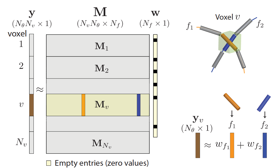
Figure 1. SpMV operation in the LiFE algorithm [Source: Copyright 2017 by Caiafa et al.  2017 ¹⁸ used under the CC BY 4.0 license ².]

The major challenge in solving Equation 2 is the significantly high memory requirements of the matrix $\bf M$. Even for small datasets, $\bf M$ can consume about $40$GB. In another work, the authors of LiFE proposed the ENCODE framework ⁷⁶, wherein Sparse Tucker Decomposition (STD) ⁹¹, a sparse multiway decomposition method to encode brain connectome, was used to reduce the memory consumption by approximately $40\times$. Using the STD technique, the diffusion signal contribution for a voxel ($\bf v$), $\bf M_{v}\in\mathbb{R}^{N_{\theta}\times N_{f}}$ is represented as:

(3) $$\scalebox{1.0}{$\bf M_{v}=S_{0}(v){D\Phi_{v}}$},$$

where $S_{0}(v)$ is the diffusion signal measured in absence of gradient, $\bf D\in\mathbb{R}^{N_{\theta}\times{N_{a}}}$ is a dictionary matrix for canonical diffusion atoms estimating individual streamline fiber based on their orientation and signal contribution, and $\bf\Phi_{v}\in\mathbb{R}^{N_{a}\times N_{f}}$ is a sparse binary matrix, whose column indicate primary contributing atoms in individual fibers, in that voxel. Thus, an equation for all $v$ can be re-written as:

(4) $$\scalebox{1.0}{$\bf Y=\Phi\times_{1}D\times_{2}S_{0}\times_{3}w^{T}$},$$

where $\Phi\times_{1}D\times_{2}S_{0}$ is 3D representation of matrix $\bf M$ and $\bf\Phi$ is a 3D representation $\forall\bf~{}\Phi_{v}$, with the goal to minimize the error between $\bf Y$ and $\bf y$ of Equation 1.

The optimization problem of Equation 4 is solved using sub-space Barzilie-Borwein non-negative least squares (SBBNNLS) algorithm ⁴⁵. Typically, the SBBNNLS algorithm takes more than $500$ iterations to converge, accounting for more than $92\%$ ($3$-$12$h) of the total execution time of LiFE (for the original naive sequential C language code). Given $\bf w_{0}$ as the initial weight vector, for every iteration, the weight vector is updated based on following equation:

(5) $$\scalebox{1.0}{$w^{(i+1)}=[w^{(i)}-\alpha^{(i)}\nabla g(w^{(i)})]_{+}$},$$

where gradient,

(6) $$\scalebox{1.0}{ $\nabla g(w)=M^{T}(Mw-y)$},$$

and the $\alpha^{(i)}$ step value for every even iteration is computed using,

(7) $$\scalebox{1.0}{ $\alpha^{(i)}=\dfrac{\langle\nabla\tilde{g}(w^{(i-1)}),\nabla\tilde{g}(w^{(i-1)})\rangle}{\langle M\nabla\tilde{g}(w^{(i-1)}),M\nabla\tilde{g}(w^{(i-1)})\rangle}$},$$

and for the odd iterations using,

(8) $$\scalebox{1.0}{ $\alpha^{(i)}=\dfrac{\langle M\nabla\tilde{g}(w^{(i-1)}),M\nabla\tilde{g}(w^{(i-1)})\rangle}{\langle M^{T}M\nabla\tilde{g}(w^{(i-1)}),M^{T}M\nabla\tilde{g}(w^{(i-1)})\rangle}$}.$$

The Equations 5-8 represent typical computations necessary for SBBNNLS of LiFE, also shown in Algorithm 1. Note that the tilde sign over gradient $\tilde{g}$ and ”$+$” subscript in Equation 5 indicates projection to positive space, i.e., negative values are replaced by zeros.

Algorithm 1 SBBNNLS algorithm used in the LiFE algorithm
(rewritten to represent matrix computations)

1:Given $\bf M$ as a connectome matrix, $\bf b$ as demeaned diffusion signal, and $\bf w^{0}$ (a vector) as initial approximation

2:For $i\leftarrow 0,N-1$

3:The gradient descent method is performed to update weight vector using following computation:

$$\bf w^{(i+1)}=[w^{(i)}-\alpha^{(i)}w^{{}^{\prime}}]_{+}$$

4:Gradient is calculated using:

$$\bf y=(Mw^{(i)}-b)$$

$$\bf w^{{}^{\prime}}=M^{T}y$$

5:The $\bf\alpha^{(i)}$ value is computed for different iterations as follows: (a) ODD iteration:

$$\bf v^{{}^{\prime}}=Mw^{{}^{\prime}}$$

$$\bf\alpha^{(i)}=\dfrac{\langle w^{{}^{\prime}},w^{{}^{\prime}}\rangle}{\langle v^{{}^{\prime}},v^{{}^{\prime}}\rangle}$$

(b) EVEN iteration:

$$\bf v^{{}^{\prime}}=Mw^{{}^{\prime}}$$

$$\bf v^{{}^{\prime\prime}}=M^{T}v^{{}^{\prime}}$$

$$\bf\alpha^{(i)}=\dfrac{\langle v^{{}^{\prime}},v^{{}^{\prime}}\rangle}{\langle v^{{}^{\prime\prime}},v^{{}^{\prime\prime}}\rangle}$$

6:End For

 $\bf\langle v,v\rangle$ is a scalar dot product of a vector $\bf v$.
$\bf{}^{\prime}+^{\prime}$ sign in subscript indicates $\bf w$ is projected to positive space.
$\bf{}^{\prime}\sim^{\prime}$ sign over gradient indicates the gradient is projected to the positive space.

2.2. Matrix Computations using Sparse Tensor Decomposition

The SBBNNLS algorithm involves two compute-intensive SpMV operations involving the matrix $\bf M$, i.e., $\bf Mw$ and $\bf M^{T}y$. On an average, every iteration (even or odd iteration) of SBBNNLS requires the $\bf Mw$ operation twice and $\bf M^{T}y$ $1.5$ times. In Figure 2, it is shown how these simple SpMV operations are transformed to a complex sequence of operations once the matrix $\bf M$ is decomposed to a sparse format using STD. The sparse tensor ($\bf\Phi$) stores non-zero indices, (atomsPtr, voxelsPtr and fibersPtr), along with the values vector (valuesPtr). In Figure 3, one can observe that the three indirection vectors of the $\bf\Phi$ tensor — atomsPtr, voxelsPtr and fibersPtr, redirects to the dictionary matrix DPtr, demeaned diffusion signal vector YPtr and weight vector wPtr respectively. The detailed algorithm for $\bf Mw$ and $\bf M^{T}y$ matrix operations are described in ¹⁸. The number of iterations of the outermost loop depends on the number of coefficients ($\bf N_{c}$) representing the non-zero indices in the $\bf\Phi$ tensor or the size of the atomsPtr/voxelsPtr/fibersPtr vectors. The number of iterations of the innermost loop depends on the diffusion directions ($\bf N_{\theta}$). Note that the innermost loop of $\bf Mw$ and $\bf M^{T}y$ corresponds to daxpy and dot-product operations respectively. It is also important noting that the wPtr vector is projected to the positive space; hence, the wPtr vector becomes sparser as it is updated after the execution of each iteration of SBBNNLS (negative values are replaced by zeros due to non-negativity property of SBBNNLS).

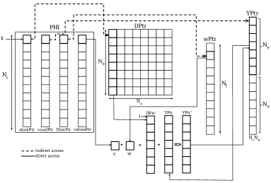
(a) $\bf y=Mw$ performing diffusion signal computation (DSC).

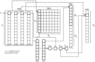
(b) $\bf w=M^{T}y$ performing weight computation (WC).

Figure 2. Block diagrams of SpMV operations used in the LiFE algorithm

⬇

1void M_times_w_sub(

2 double YPtr[], double atomsPtr[], double voxelsPtr[],

3 double fibersPtr[], double valuesPtr[], double DPtr[],

4 double wPtr[], int nTheta, int nVoxels, int nCoeffs){

5 int k, i, atom_index, voxel_index;

6 double val;

7 for(k = 0; k < nCoeffs; k++){

8 atom_index = (int)(atomsPtr[k]-1)*nTheta;

9 voxel_index = (int)(voxelsPtr[k]-1)*nTheta;

10 for(i = 0; i < nTheta; i++){

11 YPtr[voxel_index]= YPtr[voxel_index]+DPtr[atom_index]

12 * wPtr[(int)fibersPtr[k]-1] * valuesPtr[k];

13 atom_index++;

14 voxel_index++;

15 }

16 }

17 return;

18}

(a) $\bf y=Mw$: Diffusion signal computation (DSC)

⬇

1void Mtransp_times_b_sub(

2 double wPtr[], double atomsPtr[], double voxelsPtr[],

3 double fibersPtr[], double valuesPtr[], double DPtr[],

4 double YPtr[], int nFibers, int nTheta, int nCoeffs){

5 int k, i, atom_index, voxel_index;

6 double val;

7 for (k = 0; k < nCoeffs; k++){

8 val = 0;

9 atom_index = (int)(atomsPtr[k]-1)*nTheta;

10 voxel_index = (int)(voxelsPtr[k]-1)*nTheta;

11 for (i = 0; i < nTheta; i++){

12 val = val + DPtr[atom_index] * YPtr[voxel_index];

13 atom_index++;

14 voxel_index++;

15 }

16 val = val * valuesPtr[k];

17 wPtr[(int)fibersPtr[k]-1] = wPtr[(int)fibersPtr[k]-1] + val;

18 }

19 return;

20}

(b) $\bf w=M^{T}y$: Weight computation (WC)

Figure 3. Original sequential CPU code for the SpMV operations used in the LiFE algorithm ⁷⁶.

3. Problem and Challenges

In this section, we discuss problems and challenges associated with optimizing the SpMV operations used in the SBBNNLS algorithm.

3.1. Large dataset

In Equations 5-8, we observe that there are two major SpMV operations involved, namely, $\bf y=Mw$ and $\bf w=M^{T}y$. The size of the matrix $\bf M$ depends on parameters such as the number of voxels ($\bf N_{v}$), the number of fascicles ($\bf N_{f}$) and the number of diffusion directions ($\bf N_{\theta}$). The number of diffusion direction varies from $10$-$300$, voxels range from $10^{5}$ to $10^{6}$ and fibers from $10^{5}$ to $10^{7}$; therefore, the memory consumption may range from a few GBs to PBs. Thus, the matrix will typically not fit in commonly used memory systems. The authors of the LiFE application analyzed the connectome matrices and found that they are highly sparse in nature ⁷⁷; ⁷⁶. Hence, they proposed a low-rank Sparse Tucker Decomposition (STD) ⁹¹ based approach to represent the matrix $\bf M$ in a sparse tensor format and decompose it using domain-specific information. After decomposition, a new challenge of multiple irregular accesses is introduced, and this is discussed later in this section.

3.2. Architecture-specific Challenges

We will discuss some architecture-specific challenges posed in optimizing the SpMV operations of SBBNNLS.

Multi-core architecture:

In multi-core architectures, the processor can execute multiple independent instructions in parallel, hence improving the speed of a program. Shared memory multi-core architectures uses a multi-level cache memory to hide latency and reduce memory bandwidth utilization.

Improving data reuse: Shared memory multi-core architectures uses multi-level cache memory to minimize the delay caused due to memory latency. Hence, the data accessed multiple times should be reused optimally before eviction from the cache memory.

Exploiting coarse-grained parallelism: Coarse-grained parallelism is splitting of large chunk of a program so that the communication is minimized across the core. However, the coarse-grained parallelism requires load balancing so that no core remains idle.

Exploiting fine-grained parallelism: Fine-grained parallelism is spitting small chunks of programs to facilitate load balancing. However, faces a shortcoming of overhead caused due to usage of synchronization barrier.

GPU architecture:

Modern GPUs are massively parallel, multi-threaded, multi-core architectures with a memory hierarchy significantly different from CPUs. Exploiting this parallelism and the various levels of the memory hierarchy on a GPU is key to effectively optimizing the SpMV operations of SBBNNLS.

Exploiting massive parallelism: An appropriate partitioning and mapping of threads to a thread block or a grid is essential to exploit the massive parallelism on GPUs. One of the challenges here is to reduce the overhead of communication across the thread blocks and warps/threads of a thread block.

Efficiently using the GPU memory model: The SMs of a GPU share global memory, whereas local memory is allocated for a single thread. Shared memory is used for sharing data among threads of a thread block. A GPU provides multiple levels in its memory hierarchy to minimize the usage of memory bandwidth.

Coalesced memory accesses: Global memory accesses are grouped such that consecutive threads access successive memory location. When the threads of a warp access memory contiguously, the access is considered fully coalesced otherwise considered partially coalesced access. Coalesced memory accesses helps to reduce memory bandwidth requirement by loading local memory in as few memory transactions.

3.3. Indirect Array Accesses

As discussed in Section 2.2, after STD-based tensor decomposition, the SpMV operations of LiFE have several indirect array accesses. The challenges that arises for CPUs due to unstructured accesses are following: (a) the data reuse is low, hence memory bandwidth is poorly utilized, and (b) the code is executed sequentially to avoid data races that occur due to the dependent accesses. For GPUs, these irregular references (a) hinder the utilization of massive parallelism of GPUs since synchronization and an atomic operation is required to avoid data races, and (b) hamper the usage of various fast GPU memory spaces and coalesced memory accesses. These are thus the main challenges in optimizing the SpMV operations of the LiFE algorithm on general-purpose multi-core and GPU systems.

4. Optimizations

In this section, we discuss details of the techniques we incorporate to optimize the SpMV operations used in the LiFE algorithm. Firstly, we discuss target-independent optimization techniques, followed by target-specific optimizations for parallel architectures such as multi-core and GPU systems. We denote the SpMV operations for computing the diffusion signal ($\bf y=Mw$) with DSC and the weight ($\bf w=M^{T}y$) with WC. Also, in the discussion, wherever we refer to a sub-vector of a vector (Figure 4), it corresponds to any contiguous part of a sorted indirection vector having the same element value.

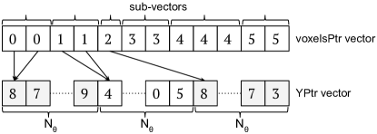
Figure 4. Sub-vectors of the voxelsPtr indirection vector

4.1. Target-independent optimizations

This section introduces target-independent optimizations such as: (1) basic compiler optimizations to avoid unnecessary and redundant computations, (2) various data restructuring methods for inducing a potential regularity in the irregular accessed data; also contributing to make further optimizations valid and fruitful, and (3) different ways to partition computations among parallel threads to effectively exploit parallelism with low synchronization overhead.

4.1.1. Basic Compiler Optimizations:

In this sub-section, we discuss some of the standard compiler optimizations that we incorporate to obtain trivial performance improvement.

Removing redundant computation:

The dictionary matrix (DPtr) and the demeaned diffusion signal matrix (YPtr) are used in the vector format for the SpMV operations (refer to Figure 3). Therefore, to compute the actual offset of these vectors, we multiply the number of diffusion direction ($\bf N_{\theta}$) with the elements of the atomsPtr and voxelsPtr indirection vectors. The original sequential CPU code computes the actual offset for every iteration of the SpMV operations of the SBBNNLS algorithm. However, we removed this redundant computation, by computing it one time before the start of SBBNNLS in the MATLAB code of LiFE. This reduced the overhead of computing the actual offsets for DPtr and YPtr in the SpMV computations.

Loop-invariant code motion:

Loop-invariant code motion optimization is utilized when a code fragment performs the same operation and computes the same output value for the different iterations of a loop, then that code fragment is hoisted out of the loop. In LiFE, the DSC operation computes the product of the weight vector (wPtr) and the values vector (valuesPtr), which remains same for the innermost loop of SpMV operations. Hence, this code fragment is hoisted out and its result is stored in a temporary variable to utilize it across the several iterations of the loop. Thus, this optimization reduced the overhead of computing the invariant-code from several times for the innermost loop to one time.

Strength reduction for arrays:

Some expressions that take more memory and CPU cycles to execute, can be compensated by an equivalent though less expensive expression. In LiFE application, the indirection vectors such as atomsPtr, voxelsPtr and fibersPtr are stored and passed as a double precision data type, and used as an index (after explicit type conversion to integer) for the DPtr, YPtr and wPtr vectors respectively. Thus, to reduce memory consumption and exploit a less expensive expression for these double precision indirection vectors, they are casted to the integer data type. This optimization is incorporated before the start of SBBNNLS in the MATLAB code and utilized across the several iterations of SBBNNLS. In addition to that, this optimization helped to cut down the data transfer overheads on GPUs due to the reduced size of the indirection vectors.

These simple and straightforward optimizations can be incorporated for both the DSC and WC operations without much effort.

4.1.2. Data Restructuring:

The LiFE algorithm is highly irregular due to the presence of multiple indirectly accessed arrays. In Figure 2, we observe that due to the STD-based representation of the matrix $\bf M$ in SpMV, three indirection vectors are involved — atomsPtr, voxelsPtr and fibersPtr, redirecting to the DPtr, YPtr and wPtr vectors respectively. These indirect array accesses procure low data reuse and prove to be a major hindrance in code parallelization as well; thus, they are a major bottleneck in optimizing the SpMV.

After analyzing the sparse datasets of LiFE, we observe that there exist several element values of an indirection vector redirecting to the same location of an indirectly accessed vector. Therefore, this is a potential source to exploit data locality. To utilize this property of the sparse datasets, we restructure the Phi tensor ($3$-D sparse representation of $\bf M$, represented by $\bf\Phi$) data based on an indirection vector to leverage regular data access patterns. If the $\bf\Phi$ tensor is restructured based on one of the indirection vectors (for example voxelsPtr), then the other indirection vectors (such as atomsPtr and fibersPtr) are accessed irregularly. Hence, a major challenge in optimizing this irregular application is to identify a near-optimal method to restructure with low runtime overhead. Thus, to achieve high performance for an SpMV operation, we determine the data restructuring to be incorporated at runtime based on the choice of a dimension (such as atom, voxel or fiber). We now discuss different data restructuring choices coupled with their strengths and weaknesses.

Atom-based Data Restructuring:

In the atom-based data restructuring method, we sort the atomsPtr vector, and depending on that, the $\bf\Phi$ tensor is restructured by reordering the voxel, fiber, and values dimensions. This method captures data reuse for the dictionary vector DPtr in both the DSC and WC operations; but it leads to poor data reuse along the other two indirectly accessed dimensions, that is, voxel and fiber.

Voxel-based Data Restructuring:

In the voxel-based data restructuring method, we sort the voxelsPtr vector, and depending on that, the $\bf\Phi$ tensor is restructured by reordering the atom, fiber, and values dimensions. This data restructuring method captures data reuse for the demeaned diffusion signal vector YPtr in the DSC and WC operations; but it leads to poor data reuse along the other two indirectly accessed dimensions, atom and fiber.

Fiber-based Data Restructuring:

In the fiber-based data restructuring method, we reorder fibersPtr, and depending on that, the $\bf\Phi$ tensor is restructured by reordering the atom, voxel, and values dimensions. The fiber-based approach captures data reuse for the wPtr vector. However, this approach loses a chance to capture data reuse for the vectors YPtr and DPtr. By inspection we found that YPtr and DPtr vectors captures a much better regular data access pattern compared to wPtr. Thus, we skip the fiber-based data restructuring for further analysis.

Hybrid Data Restructuring:

Hybrid data restructuring technique is a merger of the atom-based and the voxel-based data restructuring methods. In this technique, we first execute the DSC and WC operations for both the atom-based and the voxel-based restructuring method three times, and based on the average execution time, we select a dimension that achieves better performance for an SpMV operation. Therefore, we obtain data reuse along the atom dimension or the voxel dimension. Then, the $\bf\Phi$ tensor is restructured again by reordering the sub-vectors of the selected dimension, to capture a chance of data reuse along the other dimension (that is, other than the selected dimension). This technique will be useful for very large datasets. However, currently for this method, the performance improvement is almost negligible due to the data access patterns of the low-resolution datasets used by us and additionally, this technique has a high overhead of an additional data restructuring. Hence, we skip the hybrid-based restructuring for further evaluation as we use only low-resolution datasets (having small memory utilization) for our evaluation.

Another advantage of data restructuring besides from that of significant improvements in data reuse due to regular accesses is that the other optimizations to exploit parallelism and reduce synchronization overheads (discussed later in this section) become valid and profitable. Therefore, data restructuring play a key role to optimize the SpMV operations of LiFE.

The data restructuring to be incorporated is dependent on the input dMRI data and other parameters (such as the number of voxels and fibers) along with a tractography algorithm used. Therefore, we automate the determination of the data restructuring at runtime, by choosing a technique having lower average execution time for three runs. We included the data restructuring optimization in the LiFE algorithm’s MATLAB implementation before invoking the SBBNNLS algorithm, so that the overhead ($3$-$5\%$ of the total execution time of SBBNNLS) is amortized across several iterations of the non-negative least-squared algorithm. Note that for a different architecture and an SpMV of LIFE, the data restructuring technique that obtains a near-optimal performance may vary.

4.1.3. Computation Partitioning:

Post data restructuring, the other problem in improving performance of the SpMV operations was the usage of an atomic operation, which was required due to parallel threads performing a reduction in the DSC and WC operations (Figure 3). This causes a high synchronization overhead at runtime, detrimental to the exploitation of massive parallelism on multi-cores and GPUs. We note that the communication among threads can be reduced by mapping computations of the outermost loop of SpMV to a single thread based on the coefficient ($\bf N_{c}$) parameter of the LiFE, or on the atomsPtr or the voxelsPtr dimension. Thus, another major challenge in optimizing the SpMV operations is to determine a method to partition computations for effectively exploiting parallelism and further improving the data reuse for the YPtr and DPtr vectors. We discuss various approaches to handle the computations performed by each thread block in addition to their merits and demerits in detail.

Coefficient-based computation partitioning:

In the coefficient-based computation partitioning technique, a single thread handles computations of a single coefficient or in other words single non-zero value of the sparse tensor ($\bf\Phi$). The parallelism provided by multi-cores and GPUs can be effectively used by the coefficient-based technique, but this leads to a loss of data reuse for the YPtr and DPtr vectors. Additionally, as stated in Section  2.2, the wPtr vector is projected to positive space, implying that the negative values are replaced by zeros. This sparse property of wPtr is particularly useful for the DSC operation as a lot of unnecessary computations can be avoided. However, this computation partitioning technique requires usage of an atomic operation due to the reduction of the YPtr and wPtr vectors in the DSC and WC operations respectively. The coefficient-based technique also hinders incorporation of certain other optimizations discussed later in this section.

Atom-based computation partitioning:

In the atom-based computation partitioning technique, computations are partitioned across the threads based on the atom dimension, where each thread handles computations of a particular atom. Therefore, this technique obtains good data reuse for DPtr but lose an opportunity to exploit data reuse for YPtr. Note that the atom-based computation partitioning uses the atom-based data restructuring.

Voxel-based computation partitioning:

In the voxel-based partitioning technique, computations are partitioned across the voxels, where each thread handles computations of one voxel. In this way, the voxel-based partitioning obtains excellent data reuse for YPtr (as it is accessed twice due to reduction) but lose an opportunity to exploit data reuse for DPtr. Note that the voxel-based computation partitioning uses the voxel-based data restructuring.

The disadvantage of using the atom-based and the voxel-based techniques are (1) all iterations associated with a sub-vector of voxel or atom dimension are executed sequentially; therefore, this leads to a loss to fully utilize the sparse property of wPtr, and (2) each thread block handles several iterations depending on the size of a sub-vector, where the size may vary from one to thousands of iterations; hence, this induces load imbalance. Therefore, due to the moderate parallelism of multi-core CPUs, the load imbalance might be more prominent in them. Thus, to tackle the load imbalance in CPUs, we propose a new technique discussed later in Section 4.2.1.2. However, on GPUs, the load imbalance issue does not impact much because the number of iterations of the outermost loop ($\bf N_{c}$) in the SpMV operations is extremely large compared to the maximum possible thread blocks that can be scheduled to even the modern GPUs.

Therefore, this optimization helped in exploiting coarse-grained parallelism with excellent data reuse. We also observed that avoiding the atomic operation improves the performance considerably than taking advantage of the sparse property of wPtr. Thus, by performing experiments on the datasets used by us, we found that for DSC the coefficient-based partitioning is favourable for CPUs and the voxel-based partitioning is favourable for GPUs, whereas for WC the coefficient-based technique is favourable for both CPUs and GPUs.

4.2. Target Specific Optimizations

In this sub-section, we present target-specific optimization techniques to optimize SpMV operation of LiFE on multi-core and GPU architectures.

4.2.1. CPU-specific Optimizations:

Firstly, we discuss benefits and applicability of incorporating target-independent optimizations on CPUs. Then we introduce CPU-specific optimizations such as efficient synchronization-free thread mapping to utilize coarse-grained parallelism with reduced load imbalance and usage of BLAS library calls to exploit fine-grained parallelism.

4.2.1.1 Target-independent optimizations on CPUs:

In Section 4.1, we discussed three target-independent optimizations for SpMV operations of LiFE. The basic compiler optimizations presented are directly applicable to obtain trivial performance improvement on CPUs. The data restructuring optimization helped to enhance data reuse for YPtr and DPtr vectors in SpMV operations, and further assisted to validate parallelism. Next, we presented different ways to partition computations among the parallel threads to exploit coarse-grained parallelism. However, this optimization aggravated the issue of load imbalance for atom-based and voxel-based partitioning, and an issue of high synchronization overhead for the coefficient-based partitioning due to the usage of an atomic operation to avoid data races. It is difficult to improve the load balance for the atom-based and voxel-based partitioning methods; however, for the coefficient-based partitioning, the overhead issue can be addressed if the atomic operation is evaded. Hence, to tackle this issue we propose a CPU-specific optimization, which is discussed next in this section.

4.2.1.2 Efficient Synchronization-free Thread Mapping:

Earlier in Section 4.1.3, we discussed various ways to partition computations to the parallel threads. We concluded that for both the SpMV operations, the atom-based and the voxel-based partitioning techniques were not profitable due to the load imbalance issue. In addition to that, the atom-based and voxel-based methods required an atomic operation due to the reduction of YPtr vector in DSC operation and wPtr vector in WC operation respectively. Whereas, the coefficient-based did not have a prominent load imbalance issue but still it was not profitable due to the usage of an atomic operation.

For WC operation, we observe that for different computation partitioning techniques, the performance is influenced due to the usage of an atomic operation for the reduction of wPtr; although, based on experiments we discovered that the usage of the atomic operation did not deteriorate the performance much. We found that coefficient-based partitioning is the best choice among the other methods because it exhibits a much better load balance. However, for DSC, we observed that there was a significant drop in performance due to the usage of atomic operation (for all the partitioning methods) and the load imbalance issue (for atom and voxel based methods). Thus, using the coefficient-based partitioning method, we tackle this issue by proposing an efficient synchronization-free thread mapping technique to exploit coarse-grained parallelism without the usage of an atomic operation to improve the performance of DSC.

In Figure 5, we observe the usage of coefficient-based splitting technique for the different data restructuring methods for DSC. Figure 5a shows the atom-based restructuring technique reorders the voxelsPtr vector in such a way that there are high chances of data race at runtime; hence, this method exhibits poor performance due to requirement an atomic operation to avoid data race. Figure 5b shows that the voxel-based technique has a low chance of data dependence but cannot be eliminated completely; hence, this technique too requires an atomic operation. However, we found that there only two instances might occur for a sub-vector of the voxelsPtr vector when the voxel-based data restructuring method is employed. These instances are: (1) the entire sub-vector is scheduled to the same thread; hence, it causes no issue due to sequential execution of the iterations of the sub-vector (case 1 of Figure 5b), and (2) the sub-vector is split across the two threads (case 2 of Figure 5b); therefore, for this case an atomic operation is required due to a chance of data dependence at run-time.

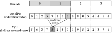
(a) atom-based data restructuring

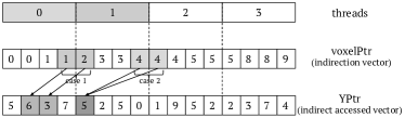
(b) voxel-based data restructuring

Figure 5. The diagram represents the atomsPtr unstructured vector redirects to the YPtr vector. (a) voxelPtr indirection vector is irregular when reordered based on the atom dimension (b) voxelPtr indirection vector is structured when reordered based on voxel dimension. The case 1 represents a sub-vector of the voxelPtr scheduled completely to a single threads. Whereas, the case 2 represents a sub-vector of the voxelPtr split across the two threads.

To tackle this issue, we ensure that the sub-vector of the voxelsPtr vector is scheduled to the same thread with a low load imbalance. In Figure 5b, we can observe in the case 2 that the sub-vector (with $4$ value) is split across the threads $1$ and $2$. To avoid any chance of occurrence of conflicting access, the sub-vector has to be scheduled to either of the one thread. If the sub-vector is scheduled to the thread-1 then it will compute two additional computations, whereas if the sub-vector is scheduled to the thread-2 then it will compute only one additional computation. Hence, scheduling the sub-vector to the thread-2 will help to reduce the load imbalance. The small overhead of load imbalance is a necessary trade-off considering the reduction in execution time obtained for parallel execution of the DSC operation without the usage of an atomic operation.

Thus, to exploit the coarse-grained parallelism for the DSC operation without atomic operation and with reduced load imbalance, we proposed an efficient synchronization-free thread mapping using the coefficient-based partitioning and the voxel-based data restructuring method.

4.2.1.3 Mapping to BLAS calls:

Basic linear algebra subroutines (BLAS) packages are often hand-optimized to obtain close to peak performance on various hardware. It is thus useful to leverage these automatically in a DSL setting. We make use of optimized BLAS call in the SpMV operations of the SBBNNLS algorithm. BLAS call improved the overall performance of the LiFE algorithm significantly. We discuss usage of a BLAS call in each of the SpMV operations of SBBNNLS.

BLAS call for DSC operation: The code fragment in the innermost loop of DSC (refer to Figure 3a) corresponds to scalar-vector product. We substitute the code fragment with the daxpy BLAS call to obtain significant performance improvement. In the BLAS call, dictionary vector (DPtr) is used as an input vector and the product of a value in the weight vector (wPtr) and the values vector (valuesPtr) is used as a scalar input. The output is used to update the demeaned diffusion signal vector (YPtr).

According to the SBBNNLS stated in Algorithm 1, wPtr is projected to the positive space; hence, due to this property of wPtr the negative values are replaced by zeros. Therefore, the wPtr vector is sparse in nature. Hence, in the DSC operation, if the scalar value obtained from the product vector wPtr and vector valuesPtr is zero then invoking the BLAS call is futile and should be avoided to refrain from unnecessary computations.

BLAS call for the WC operation: The code fragment in the innermost loop of WC (refer to Figure 3b) corresponds to vector-vector dot product. We substitute the code fragment with the dot BLAS call to obtain performance improvement. In dot BLAS call, the YPtr and DPtr vectors are used to update the wPtr vector. However, in contrast to the DSC operation, the execution time remains almost the same throughout SBBNNLS.

Usage of BLAS call provided fine-grained parallelism for the SpMV operations and improved the performance considerably. Particularly, the DSC operation was greatly benefited by the usage of the BLAS call.

To summarize the optimization of SpMV on CPUs, first we performed the target-independent optimizations, followed by the CPU-specific optimizations to obtain a highly optimized CPU code for the SpMV operations of SBBNNLS. We also extended the PolyMage DSL to incorporate all the optimization presented in this section to automatically generate optimized parallelized code involving the sparse representation of the SpMV operations of SBBNNLS and obtained comparable performance to that of the manually optimized version (CPU-opt). We will discuss more on the DSL extension in Section 5. Note that some of the CPU optimizations require runtime data analysis such as the optimization presented in Section 4.2.1.2. Thus, it could not be incorporated for the automated CPU code version and as a result the automated code version could not achieve the similar performance compared to that of the hand-optimized CPU code version.

4.2.2. GPU-specific Optimizations:

Firstly, we discuss benefits and applicability of incorporating target-independent optimizations on GPUs. Then, we present various GPU-specific optimizations to optimally map threads at the granularity of warps, thread blocks and grid to obtain fine-grained parallelism and improved data reuse. We use GPU code developed by Madhav ⁵⁷, shown in Figure 6, as a reference GPU code version.

4.2.2.1 Target-independent optimizations on GPUs:

In Section 4.1, we discussed a number of target-independent optimizations for SpMV operations. For GPUs, the basic compiler optimizations presented is useful to obtain minor performance. The data restructuring optimization proposed captured enhanced data reuse for YPtr and DPtr vectors, and further aided to legitimize parallelism. Following that, we presented different ways to partition computations among the parallel threads to exploit coarse-grained parallelism. However, this optimization had similar issues for a GPU that we discussed in Section 4.2.1.1 for a CPU; although, the issue of the load balance discussed earlier for a CPU is not prominent for a GPU due to its massive parallelism. Thus, we do not introduce any new optimization to tackle load imbalance issue for the GPUs and take a step forward to exploit fine-grained parallelism in the SpMV operations.

⬇

1__global__ void M_times_w(

2 const long *atomPtr, const long *voxelPtr,

3 const long *fibersPtr, const double *valuesPtr,

4 const double *DPtr, const double *wPtr,

5 const int nTheta, const long nVoxels,

6 const long nCoeffs, double *yPtr) {

7 long k = threadIdx.x + blockIdx.x * blockDim.x;

8 long offset = 0;

9 long stride = gridDim.x * blockDim.x;

10 while ((k + offset) < nCoeffs) {

11 long atom_index = atomsPtr[k + offset];

12 long voxel_index = voxelsPtr[k + offset];

13 double val1 = wPtr[fibersPtr[k + offset]];

14 double val2 = valuesPtr[k + offset];

15 for (int i = 0; i < nTheta; i++) {

16 atomicAdd(&YPtr[voxel_index][i], DPtr[atom_index][i]

17 * val1 * val2);

18 }

19 offset += stride;

20 }

21 return;

22}

(a) C++/CUDA GPU code for $\bf y=Mw$

⬇

1__global__ void Mtransp_times_b(

2 const long *atomPtr, const long *voxelPtr,

3 const long *fibersPtr, const double *valuesPtr,

4 const double *DPtr, const double *YPtr,

5 const long nFibers, const int nTheta,

6 const long nCoeffs, double *wPtr) {

7 long k = threadIdx.x + blockIdx.x * blockDim.x;

8 long offset = 0;

9 long stride = gridDim.x * blockDim.x;

10 while ((k + offset) < nCoeffs) {

11 double val = 0;

12 long atom_index = atomsPtr[k + offset];

13 long voxel_index = voxelsPtr[k + offset];

14 for (int i = 0; i < nTheta; i++) {

15 val += DPtr[atom_index][i] * YPtr[voxel_index][i];

16 }

17 val = val * valuesPtr[k + offset];

18 atomicAdd(&wPtr[fibersPtr[k + offset]], val);

19 offset += stride;

20 }

21 return;

22}

(b) C++/CUDA GPU code for $\bf w=M^{T}y$

Figure 6. Reference GPU code for the SpMV operations used in the SBBNNLS algorithm

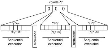
(a)

(b)

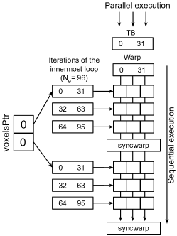
(c)

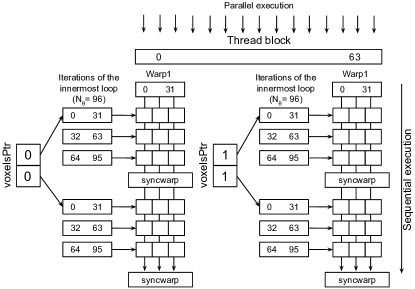
(d)

Figure 7. (a) Sequential execution of iterations of a sub-vector of the voxelsPtr vector scheduled to single thread block. (b) Parallel execution of innermost loop ($N_{\theta}$=96) and sequential execution of a sub-vector of voxelsPtr scheduled to three warps and a single thread block. (c) Parallel execution of innermost loop ($N_{\theta}$=96) and sequential execution of a sub-vector of the voxelsPtr scheduled to single warp and a single thread block. (d) Parallel execution of innermost loop ($N_{\theta}$=96) and sequential execution of two distinct sub-vectors of the voxelsPtr scheduled to single warp and a single thread block.

4.2.2.2 Exploiting Fine-grained Parallelism:

The reference optimized GPU approach executes the innermost loop of both the SpMV operations sequentially (Figure 6). It was performed due to the indirect array accesses of the SpMV operations and the concurrent scheduling of multiple iterations of the outermost loop to a single thread block; hence, the innermost loop had to be executed sequentially to avoid a data race. Thus, due to these reasons, the reference GPU approach missed out an important opportunity to exploit fine-grained parallelism. However, with the aid of resources and instructions provided by a GPU architecture, we could exploit fine-grained parallelism; hence, it helps in obtaining substantial performance improvement in both the SpMV operations. We discuss the different techniques to achieve fine-grained parallelism in the DSC and WC.

Shared memory: Shared memory is an on-chip explicitly addressed memory with significantly lower memory latency than local and global memories of GPUs. It is key in reducing memory access time when data accessed by the threads of a thread block exhibit reuse.

In Figure 6a, we notice in the DSC code that the innermost loop (line $15$) performing the daxpy operation is executed sequentially. We used shared memory to execute the iterations of the innermost loop in parallel, though with the usage of a synchronization barrier. However, later in Section 4.2.2.3, we will note that the threads can be executed without the employment of a memory fence. The added advantage of using the shared memory is reduced memory bandwidth requirements obtained due to data reuse of YPtr. Also, note that the size of shared memory required depends on the diffusion direction ($\bf N_{\theta}$).

Shuffle instruction: Parallel threads of a thread block share data using shared memory. However, NVIDIA’s Kepler architecture introduced a new warp-level instruction, named, shuffle instruction (SHFL) ²⁹, to be utilized when the data is to be shared directly among the parallel threads of a warp. It leads to a considerable reduction in latency without the use of shared memory.

In Figure 6b, we observe in the WC code that the innermost loop (line $14$) performing dot-product operation is executed sequentially. The dot-product involves two sub-operations — (1) multiply corresponding elements of the vectors, which can be performed in parallel, (2) perform a reduction, which is performance bottleneck if performed sequentially. A popular method to perform reductions in GPUs is to use shared memory. This method however is dependent on the size of shared memory and requires the employment of a memory fence, thereby hurting performance. An alternative method is to use the SHFL instruction ²⁹. It helps to share data directly among the parallel threads of a warp, but requires the usage of a synchronization barrier and shared memory, across the warps of a thread block. However, later in Section 4.2.2.3, we will tackle the synchronization bottleneck as well. Using SHFL, we parallelized the dot-product to significantly reduce the execution time of WC.

Thus, in Figure 7b, we can observe that after incorporating the fine-grained parallelization, the innermost loop of an SpMV operation is executed in parallel, where each thread block handles the iterations of a single sub-vector of voxelsPtr. Note that the computations associated with an iteration of the sub-vector are executed in parallel. However, the computations across the iterations are executed sequentially, requiring the syncthread barrier in between the iterations. We tried to replace the daxpy computation in the innermost loop of the DSC code and the dot-product computation in the innermost loop of the WC code with appropriate cuBLAS library calls, but were unsuccessful due to the difficulty in interfacing this from MATLAB.

4.2.2.3 Reduce Synchronization Overhead by using Warp-based Thread Execution:

On NVIDIA GPUs, a warp is a collection of a certain number of threads (typically $32$) executing the same code in lock-step and is best used when each thread follows the same execution path. When there are a number of warps sharing data or performing dependent pieces of computation, those pieces need to be synchronized and this could impact performance. As discussed earlier in Section 4.2.2.2, the SpMV operations of the LiFE algorithm face a similar challenge.

In Figure 7b, we observe that the iterations of the innermost loop of the SpMV operations executing in parallel require syncthread barrier across the warps of a thread block. However, by transforming the innermost loop, multiple warps can be replaced by a single warp. Note that the innermost loop parameter depends on $\bf N_{\theta}$, which is typically a multiple of $32$ for most of the dMRI datasets ($96$ for dMRI datasets we used). So the innermost loop is transformed such that the $32$ iterations are executed in parallel by a warp, and then the next $32$ iterations are executed in parallel by the same warp, i.e., $\bf N_{\theta}$/$32$ times sequential execution (as shown in Figure 7c, $\bf N_{\theta}$=96 requires three sequential executions). The advantage of this change is that we can utilize syncwarp, a much less expensive barrier operation when compared to the syncthread barrier. This will also benefit the next set of optimizations we incorporate to optimize SpMV (discussed later in this section). However, if $\bf N_{\theta}$ is not a multiple of $32$ then the zeros are padded for the YPtr and DPtr vectors to tune their dimensions to a multiple of $32$. The overhead ($2$-$3$% of the total execution time of SBBNNLS) of padding is low considering that it is amortized across the several iterations of SBBNNLS.

4.2.2.4 Exploiting Additional Data Reuse:

Earlier in Section 4.1.3, we discussed different ways to partition computations of the outermost loop of the SpMV operations among the thread blocks. We scheduled computations of a single coefficient, voxel or atom dimension to a single thread block (Figure 7a); so that the atomic operation hindering the coarse-grained parallelism could be avoided. Despite this optimization, a thread block could not fully utilize the resources allocated by a GPU (such as shared memory and cache memory). The reasons for this were: (1) the size of $\bf N_{\theta}$ is small, and (2) only one warp is scheduled per thread block because of the optimization discussed in Section 4.2.2.3 (shown in Figure 7c).

However, we found that resources allocated for a single thread block could be utilized optimally (Figure 7d) by scheduling multiple computations of coefficients, voxels or atoms could to a single thread block. Thus, this optimization would help to effectively utilize shared memory to exploit an additional data reuse for the YPtr and DPtr vectors, thereby leads to reduction of memory bandwidth consumption. Additionally, the synchronization overhead will also reduce due to the usage of the syncwarp barrier. To obtain near-optimal performance improvements on this aspect, we empirically determined the right number of computations to be scheduled for a thread block. We found that for both the DSC and WC, four computations per thread block provided the near-optimal performance.

4.2.2.5 Loop Unrolling:

Loop unrolling is straightforward and well-known to improve performance by reducing control overhead, providing more instruction scheduling freedom, and increasing register reuse. Using loop unrolling, we achieve an additional performance improvement for the DSC operation. However, a similar performance improvement was not observed for the WC operation because the loop index was static; so the compiler might have automatically unrolled the loop. We determined the unroll factor by performing a few experiments and found eight was optimal unroll factor for the DSC. We used #pragma unroll N (where N is unroll factor) to unroll the loop corresponding to the iterations of the sub-vector of an indirection vector (example voxelsPtr) in the CUDA code of the DSC of SBBNNLS.

To summarize the optimization of SpMV on GPUs, first we performed the target-independent optimizations, followed by the GPU-specific optimizations to obtain a highly optimized GPU code for the SpMV operations of SBBNNLS.

5. Domain-Specific Language Extensions

In this section, we provide a brief overview of the PolyMage DSL and a description of the constructs we added to the DSL, in order to express sparse matrices and the related operations used in the LiFE algorithm.

⬇

1class PHI_Tensor(Function):

2 def __init__(self, _typ, _name, _dim):

3 C = _dim

4 atomPtr = Matrix(ULong, "atomsPtr", [C])

5 voxelPtr = Matrix(ULong, "voxelsPtr", [C])

6 fiberPtr = Matrix(ULong, "fibersPtr", [C])

7 valPtr = Matrix(Double, "valuesPtr", [C])

8

9 self._atomPtr = atomPtr

10 self._voxelPtr = voxelPtr

11 self._fiberPtr = fiberPtr

12 self._valPtr = valPtr

13 self._C = C

(b)

⬇

1class Sparse_M_w(Function):

2 def __init__(self, _PHI_Node, _DPtr, _YPtr,_wPtr):

3 atomPtr = _PHI_Node.atom()

4 voxelPtr = _PHI_Node.voxel()

5 fiberPtr = _PHI_Node.fiber()

6 valPtr = _PHI_Node.vals()

7

8 C = _PHI_Node.dim()

9 T = _YPtr.dimensions[1]

10

11 k = Variable(UInt,’k’)

12 i = Variable(UInt,’i’)

13

14 r1 = Interval(UInt,0,C)

15 r2 = Interval(UInt,0,T)

16

17 c1 = Condition(k,">=",0) & Condition(k,"<",C)

18 c2 = Condition(k,">=",0) & Condition(k,"<",C) \

19 & Condition(i,">=",0) & Condition(i,"<",T)

20

21 YPtr = Reduction(([k,i],[r1,r2]),([k,i],[r1,r2]),Double,"YPtr")

22 YPtr.defn = [Case(c2, Reduce( YPtr(k,i),_YPtr(voxelPtr(k),i) \

23 + (_DPtr(atomPtr(k),i)*_wPtr(fiberPtr(k)) * valPtr(k)) ,Op.Sum))]

24 YPtr._idiom = ’daxpy’

25

26self._YPtr = YPtr

27 def out(self):

28 return self._YPtr

(c)

Figure 8. (a) PolyMage code for $\bf y=Mw$ operation of LiFE (b) PolyMage construct for PHI tensor ($\bf\Phi$) to represent STD-based tensor (c) PolyMage construct for $\bf y=Mw$ operation of LiFE.

5.1. PolyMage DSL

⁷¹ developed PolyMage, a domain-specific language (DSL) and a compiler for image processing pipelines. PolyMage automatically generates optimized parallelized C++ code from a high-level language embedded in the Python. The PolyMage compiler is based on a polyhedral framework for code transformation and generation. The constructs used in the PolyMage represents a high-level code in a polyhedral format. The compiler then performs various optimizations such as loop fusion, loop tiling across various functions and also marks loop(s) parallel. Some constructs used in the PolyMage DSL are following: Parameter construct used to declare a constant value and Variable construct used to declare a variable which usually serves as labels for a function dimension. The range of a variable is declared using Interval construct. Function construct is used to declare a function mapping from a multi-dimensional integer domain to a scalar value. Conditional construct is used to specify constraints involving variables, parameters and function values. Case construct allows a conditional execution of a computation. We introduce two new constructs to support sparse matrix and the related operations used in the SBBNNLS algorithm.

5.2. New Constructs Added to PolyMage

We introduce PHI_Tensor construct to represent sparse decomposed tensor to enhance productivity. The sparse decomposed tensor consists of four vectors: three vectors atomPtr, voxelPtr and fiberPtr represents the dimensions of a non-zero value in a connectome tensor and another vector valuesPtr to represents the actual value of a non-zero index. We use Matrix construct already defined in the PolyMage to represent these four vectors (Figure 8b). Sparse_matvec construct (Figure 8c) is added to perform the sparse matrix-vector multiplication $\bf y=Mw$ operation (Figure 2a) used in the SBBNNLS algorithm of the LiFE application. We obtain a sparse decomposed matrix from the PHI_Tensor construct. Additionally the dictionary vector DPtr, the weight vector wPtr and the demeaned diffusion signal vector YPtr are obtained as a input from the user to update the YPtr vector. We use the Function construct to execute the Case construct defined in the function definition based on the $\bf c1$ and $\bf c2$ Condition construct using the $\bf k$ Variable construct. The high-level PolyMage code used to generate optimized parallelized C++ code for the sparse matrix operation of the SBBNNLS algorithm is shown in Figure LABEL:fig:polymagesparsematvec.

6. Experimental Evaluation

In this section, we describe the experimental setup, followed by various code versions and datasets we evaluated. We then present experimental results while analyzing them. We show performance improvements we achieved by incorporating the target-independent and the target-dependent optimizations for SpMV operations (presented in Section 4), then we compare our highly optimized parallelized CPU implementation and our highly optimized GPU implementation with the original sequential CPU implementation, a reference optimized GPU implementation, and ReAl-LiFE’s GPU implementation. We also compare various SpMV code implementations by varying different parameters of the dMRI datasets.

Table 1. System details 

Microarchitecture	Intel Skylake
Processors	2-socket Intel Xeon Silver 4110
Clock	2.10 GHz
Cores	16 (8 per socket)
Hyperthreading	disabled
Private caches	64 KB L1 cache, 1024 KB L2 cache
Shared cache	11,264 KB L3 cache
Memory	256 GB DDR4 (2.4 GHz)
Microarchitecture (GPU)	NVIDIA Turing
GPU	NVIDIA GeForce RTX 2080 Ti
Multiprocessors (SMs)	64
CUDA cores (SPs)	4352
GPU Base Clock	1350 Mhz
L1 cache/shared memory	96 KB
L2 cache size	5.5 MB
Memory size	11.26 GB GDDR6
Memory bandwidth	616 GB/s
Matlab version	9.5.0.944444 (R2018b)
MRtrix version	3.0
CUDA/NVCC version	10.0
NVCC version	10.0.130
Compiler	GNU C/C++ (gcc/g++) 6.3.0
Compiler flags	-O3 -ptx
OS	Linux kernel 3.10.0 (64-bit) (CentOS 7)

6.1. Experimental Setup

The evaluation was performed on an NVIDIA GeForce RTX 2080 Ti GPU and a dual-socket NUMA server with Intel Xeon Silver 4110 processor based on the Intel Skylake architecture. The complete specification is provided in Table 1. The LiFE application is originally written in MATLAB with the computationally intensive SpMV operations of the SBBNNLS algorithm written in C++/CUDA-C++ language. The reference optimized code developed by Madhav ⁵⁷, ReAl-LiFE implementation ⁴⁸, and our optimized GPU code are compiled using NVCC compiler to generate PTX code. The SpMV kernels are represented as a CUDAKernel object in MATLAB, which is used to invoke the compiled PTX code. The advantage of using the CUDAKernel object is that the same data is used across the different iterations of SBBNNLS and need not be transferred back and forth from the host to device and vice-versa. To compare the execution time of various tractography algorithms, we use MRtrix ⁹⁰ — an advanced tool to analyze the diffusion MRI data. MRtrix generates streamline tracts for numerous tractography algorithms.

6.2. Datasets

The evaluation was performed on the STN96 dMRI dataset collected at Stanford’s Center for Cognitive and Neurobiological Imaging ⁷⁵.

DS1:

dMRI data was collected at ⁷⁵. The diffusion signal was measured along the $96$ directions, with the spatial resolution of $1.5mm$ and the gradient strength of $2000s/mm^{2}$.

DS2:

dMRI data was same as DS1; however, we used MRtrix to generate streamline tracts in-house for various tractography algorithms such as: deterministic algorithm (Tensor_DTI) based on 4-D diffusion-weighted imaging (DWI) ¹⁰, probabilistic algorithm based 4-D DWI (Prob_DTI) ³⁸, fiber assigned continuous tracking (FACT) ⁶⁶, fiber orientation distribution (iFOD1) ⁹⁰, and spherical deconvolution (SD_STREAM) ⁹⁰ method. There are numerous tractography algorithms available but based on the popularity we choose these tractography algorithms for our evaluation.

6.3. Results and analysis on Multi-core System

In this sub-section, we present detailed analysis of the target-independent optimizations incorporated for the SpMV operations running on CPUs, followed by the evaluation of the CPU-specific optimizations.

6.3.1. Code Versions:

The various SpMV code implementations that we use to analyze the performance of the SBBNNLS algorithm on multi-cores are as follows:

• CPU-naive (Figure 3) is the original sequential code for the DSC and WC SpMV operations developed by Caiafa and Pestilli ⁷⁶.

• CPU-naive-withBLAS is a variant of CPU-naive implementation with code fragments replaced by an appropriate BLAS call.

• CPU-naive-par-withoutBLAS is a variant of the CPU-naive version, parallelized by marking the outermost loop parallel though having statements with a chance of conflicting data accesses marked atomic. Note that the BLAS calls cannot be marked atomic. Therefore, the BLAS calls cannot be replaced by the code fragment in Naive-par-withoutBLAS code version.

• CPU-opt is our highly parallelized optimized C++ code implementation with all target-independent optimizations presented in Section 4.1 and the CPU-specific optimizations presented in the Section 4.2.1.

• CPU-opt-atomic-withoutBLAS is a variant of CPU-opt version without usage of a BLAS call and having statements marked atomic having a chance of conflicting data dependent accesses.

• CPU-opt-withoutBLAS is a variant of CPU-opt version without usage of a BLAS call.

6.3.2. Analysis:

Table 2 shows the execution time in seconds for DSC and WC operations for different data restructuring methods performed on the CPU-naive sequential implementation. In the table, we observe that the atom-based data restructuring method is slightly better for both DSC and WC operations. Also, the execution time of DSC and WC is similar for the different iterations of SpMV. Thus, from this table we infer that the DPtr vector (redirected by the atomsPtr) captures better reuse compared to the YPtr vector (redirected by the voxelsPtr).

Table 2. Execution time for CPU-naive implementation of the SpMV operations for various data restructuring methods on Intel Xeon processor.

Iterations	SpMV operation
	DSC		WC
	Atom	Voxel	Atom	Voxel
1	8.187s	8.214s	6.320s	6.490s
100	8.490s	8.228s	6.316s	6.496s
200	8.484s	8.227s	6.315s	6.500s
300	8.465s	8.231s	6.283s	6.478s
400	8.459s	8.210s	6.286s	6.464s
500	8.452s	8.767s	6.301s	6.463s

Table 3. Execution time of CPU-naive-par-withoutBLAS implementation of SpMV for different computation partitioning + data restructuring combinations on Intel Xeon processor.

	SpMV operation
Iterations	DSC		WC
	Voxel+Voxel	Coeff+Voxel	Voxel+Voxel	Atom+Atom	Coeff+Voxel	Coeff+Atom
1	2.553s	2.040s	0.905s	0.957s	0.720s	0.678s
100	2.663s	1.785s	0.814s	0.904s	0.636s	0.682s
200	2.451s	1.778s	0.877s	0.955s	0.640s	0.666s
300	2.471s	1.787s	0.834s	1.001s	0.645s	0.673s
400	2.412s	1.778s	0.841s	0.905s	0.646s	0.665s
500	2.407s	1.783s	0.811s	0.907s	0.660s	0.667s

Table 3 shows the execution time in seconds for DSC and WC operations for different combinations of computations partitioning + data restructuring methods performed on CPU-naive-par-withoutBLAS implementation (marking the outermost loop parallel and data dependent statements marked atomic) running on $16$-core Intel Xeon processor. For DSC operation, we observe that the coefficient-based partitioning + voxel-based restructuring combination performs better due to efficient usage of the parallelism provided by CPU with a low load imbalance. In contrast, the voxel-based partitioning + voxel-based restructuring combination does not perform well due to a high load imbalance. Note that DSC operation involves reduction of YPtr (with indirection from voxelsPtr); therefore, the voxel-based technique will capture reuse twice due to read and write access, whereas the atom-based restructuring will require usage of an atomic operation for the reduction of the irregularly accessed YPtr. Thus, due to these reasons we skip the atom-based restructuring for the DSC operation. For WC operation, we observe that the coefficient-based partitioning + atom-based restructuring combination performs much better compared to the other combinations. The reason for this is that the coefficient-based partition exploits the parallelism effectively, on the other hand the atom-based data restructuring captures the data reuse efficiently. Thus, this combination is best for WC operation. Besides this, one can observe that the execution time of DSC and WC is similar for the different iterations of SpMV.

Table 4. Execution time of CPU-opt implementation of SpMV for different computation partitioning + data restructuring combinations on Intel Xeon processor.

	SpMV operation
Iterations	DSC		WC
	Voxel+Voxel	Coeff+Voxel	Voxel+Voxel	Atom+Atom	Coeff+Voxel	Coeff+Atom
1	0.534s	0.486s	0.510s	0.545s	0.482s	0.382s
100	0.147s	0.133s	0.496s	0.533s	0.442s	0.379s
200	0.124s	0.113s	0.496s	0.524s	0.432s	0.376s
300	0.126s	0.111s	0.503s	0.534s	0.428s	0.375s
400	0.139s	0.112s	0.500s	0.538s	0.446s	0.375s
500	0.122s	0.111s	0.498s	0.559s	0.426s	0.391s

Table 4 shows the execution time in seconds for DSC and WC operations performed using CPU-opt implementation (running on $16$-core Intel Xeon processor) for different computations partitioning + data restructuring combinations. We observe that for both DSC and WC, the computation partitioning + data restructuring combination that performs best is similar to that of CPU-naive-par-withoutBLAS implementation. However, the execution time is significantly lower for CPU-opt SpMV operations compared to the CPU-naive-par-withoutBLAS implementation due to the CPU-specific optimizations that we incorporated. Another interesting point to observe is that the execution time of DSC reduces as the iteration increases. The reasons for this is due the sparse property of the wPtr vector. We discuss more about it later in this sub-section.

Figure 9 reports absolute execution time in seconds for different CPU code implementations of SpMV ($\bf Mw$ and $\bf M^{T}y$) for different iterations of the SBBNNLS algorithm. We observe that by marking the outermost loop parallel in the Naive-par-withoutBLAS version achieved a speedup of $4.3\times$ over the CPU-naive version. However, it did not improve the performance significantly due to following reasons: (a) poor data locality captured for YPtr and DPtr vectors, and (b) statements marked atomic due to a chance of conflicting data accesses. We also notice that the CPU-opt-atomic-withoutBLAS version shows comparable performance with the Naive-par-withoutBLAS version for the same reasons (the statements were marked atomic), though slightly better due to the improved data reuse. For the DSC operation, we calculated the average execution time over the $500$ iterations of SBBNNLS and obtained a speedup of $12.43\times$ for CPU-opt version over CPU-opt-atomic-withoutBLAS version. However, after incorporating the target-independent optimizations and the efficient synchronization-free thread mapping optimization, we not only obtained better data reuse but were also able to mark the outermost loop parallel without the usage an atomic operation (for the DSC operation). Overall, for complete execution of SBBNNLS we obtained a speedup of $27.25\times$ and $6.33\times$ for CPU-opt version over the CPU-naive and CPU-naive-par-withoutBLAS respectively. Later in this sub-section, we will discuss more about benefit of code parallelization of the SpMV operations of LiFE.

(a) Diffusion signal computation (DSC) $\bf y=Mw$

(b) Weight computation (WC) $\bf w=M^{T}y$

Figure 9. Execution time (in seconds) of SpMV used in the LiFE with various optimizations running on Intel Xeon processor.

We also observe that mapping to a BLAS call significantly improved the performance of both the CPU-naive and the CPU-opt versions of the DSC and WC computations. We notice that for the DSC operation, as the number of iteration increases, the execution time reduces remarkably and becomes stable thereafter; the reason for this improvement is the weight vector (wPtr) becomes sparser. So when the vector wPtr is used as a scalar in the argument of the (daxpy) BLAS call, the invocation of the call is evaded to avoid unnecessary computations. We computed the average execution time of the DSC operations over $500$ iterations and obtained a speedup of $5.5\times$ for CPU-naive-withBLAS version over the CPU-naive version. Similarly, we achieved a speedup of $4.81\times$ for the CPU-opt version over the CPU-opt-withoutBLAS version. Note that in the WC operation, the similar performance improvement was not observed due the set of computations it involved.

Table 5. Total execution time (in min) up till different iterations of the SBBNNLS algorithm for a different number of cores on Intel Xeon processor. The baseline is CPU-naive version.

Code	Iters	Execution time (in min)						Speedup
			2	4	8	12	16	1	2	4	8	12	16
CPU-naive	10	5.24	5.73	3.14	1.85	1.37	1.11	1.00	0.91	1.66	2.82	3.81	4.73
	100	45.1	54.5	30.1	17.9	13.1	10.5	1.00	0.82	1.49	2.51	3.42	4.29
	500	225	271	149	88.6	65.6	52.2	1.00	0.82	1.51	2.53	3.42	4.30
CPU-opt	10	1.91	1.22	0.66	0.41	0.35	0.31	2.74	4.29	7.86	12.5	14.9	17.2
	100	14.3	8.86	4.76	2.78	2.22	1.97	3.13	5.08	9.46	16.1	20.3	22.8
	500	61.8	39.1	20.8	12.1	9.43	8.29	3.63	5.74	10.8	18.5	23.8	27.2

Table 5 shows the total execution time up till different iterations of the SBBNNLS algorithm and speedups achieved with different number of threads. We compare the performance of the CPU-naive version (also used as base version) with CPU-naive-par-withoutBLAS version and the CPU-opt version. We observe that for the Naive-par-withoutBLAS version, the speedup remains similar for the different iterations. In addition to that, as the number of threads increases the performance does not scale well. However, for the CPU-opt code version the performance improves for different iterations of the SBBNNLS algorithm. Also it is worth noting that the performance scales well up till $8$ threads due to improved data reuse, but because of NUMA effects does not scale further. As discussed earlier in this sub-section, mapping a code fragment of the DSC operation to the BLAS call leverages the sparse nature of the wPtr vector. From Table 5 the same can be seen, the more the number of iteration the better is the speedup achieved for the CPU-opt version. The CPU-naive and Naive-par-withoutBLAS code versions does not use a BLAS call; hence, the speedup remains the same for them due to the execution of the unnecessary computations.

Summarizing the results for CPUs, for the DSC operation we achieve optimal performance by incorporating the voxel-based data restructuring technique. For the WC operation, we achieve optimum performance by incorporating the atom-based data restructuring technique. Once the data was restructured, optimizations such as loop tiling and code parallelism helped obtaining coarse-grained parallelism. We achieved significantly better performance improvement by mapping to BLAS calls for exploiting fine-grained parallelism.

6.4. Results and analysis on GPU

In this sub-section, we present detailed analysis of the target-independent optimizations incorporated for the SpMV operations running on GPUs, followed by the evaluation of the GPU-specific optimizations.

6.4.1. Code Versions:

The various SpMV code implementations that we use to analyze the performance of the SBBNNLS algorithm on GPUs are as follows:

• Ref-opt is a reference optimized GPU code developed by Madhav ⁵⁷, on a similar set of CPU optimization mentioned for the CPU-opt implementation. For the SpMV operations, the Ref-opt code reorders the data based on the atom dimension to exploit data reuse and also uses the coefficient-based partitioning to achieve coarse-grained parallelism.

• ReAl-LiFE is a GPU-accelerate implementation using the voxel-based data restructuring and the voxel-based computation partitioning for both DSC and WC operations. In addition, the ReAl-LiFE implementations uses shared memory for DSC and shared memory + shuffle instruction for WC operations to achieve fine-grained parallelism with single-warp based execution.

• GPU-opt is our optimized GPU code implementation with all the optimizations mentioned in Section 4.2.2. In contrast to ReAl-LiFE implementation, we added following optimizations: (1) automated selection of the data restructuring + computation partitioning combination at run-time, (2) utilized only shuffle instruction to exploit fine-grained parallelism for WC, (3) scheduled multiple computations to a thread block, and (4) exploited the sparse property of the wPtr vector.

6.4.2. Analysis:

Table 6. Execution time of Ref-opt implementation of the SpMV operations for various data restructuring techniques on NVIDIA GPU.

Iterations	SpMV operation
	DSC		WC
	Atom	Voxel	Atom	Voxel
1	1.025s	2.087s	0.310s	0.311s
100	0.185s	0.219s	0.316s	0.320s
200	0.166s	0.190s	0.319s	0.320s
300	0.162s	0.187s	0.319s	0.320s
400	0.162s	0.186s	0.319s	0.320s
500	0.162s	0.186s	0.319s	0.320s

Table 6 reports the execution time in seconds for DSC and WC operations at different iterations of SBBNNLS for various data restructuring techniques discussed in Section 4.1.2. Evaluation was performed on the Ref-opt + data-restructure code — a modification of the Ref-opt GPU code obtained by incorporating the data restructuring optimization. We observe that the performance of the atom-based data restructuring is surprisingly better than the voxel-based data restructuring for the DSC computation. The reason for this is that the voxel-based approach achieve good data reuse; however, due to the usage of an atomic operation the overhead is high. Though, later in this sub-section, we will discern that when other optimizations are incorporated, the voxel-based data restructuring technique outruns the atom-based technique. In the case of WC, we observe that the atom-based and voxel-based restructuring techniques achieve a similar order of performance because the data reuse is obtained either for the YPtr vector or the DPtr vector.

Table 7. Execution time of Ref-opt implementation of the SpMV operations for different computation partitioning + data restructuring combinations on NVIDIA GPU.

	SpMV operation
Iter(s)	DSC		WC
	Voxel+Voxel	Coeff+Voxel	Voxel+Voxel	Atom+Atom	Coeff+Voxel	Coeff+Atom
1	0.318s	1.025s	0.311s	0.313s	0.188s	0.122s
100	0.057s	0.185s	0.318s	0.320s	0.184s	0.121s
200	0.053s	0.166s	0.321s	0.320s	0.184s	0.121s
300	0.052s	0.162s	0.321s	0.320s	0.184s	0.121s
400	0.052s	0.162s	0.321s	0.320s	0.182s	0.121s
500	0.052s	0.162s	0.322s	0.320s	0.184s	0.120s

Table 7 shows the execution time in seconds for DSC and WC operations performed using Ref-opt implementation for different combinations of computations partitioning + data restructuring methods. For DSC operation, we observe that the voxel-based partitioning + voxel-based restructuring combination performs better compared to the coefficient-based partitioning + voxel-based restructuring. As discussed earlier in Section 4.1.3, the reason for this is that the load imbalance issue on GPUs caused due to partitioning based on voxel dimension is low considering its massive parallelism. Additionally, the number of iterations of the outermost loop ($\bf N_{c}$) is much larger than maximum possible thread blocks that can be scheduled to a GPU. Hence, this combination performs good for DSC operation. In contrast to that, the coefficient-based partitioning performs poorly because of the reduction of the YPtr has dependent accesses at runtime; therefore, this partitioning method have a high synchronization overhead due to the usage of an atomic operation to avoid data races. For WC operation, the combination of coefficient-based partitioning + atom-based restructuring performs best compared to others. The reason for this is that the coefficient-based partitioning exploits parallelism of GPUs effectively, on the other hand atom-based data restructuring leverages data reuse efficiently. Also, one can observe that the execution time for both DSC and WC operations are same for different iterations of SBBNNLS; therefore, the sparse property of wPtr is not exploited efficiently by different combinations of computations partitioning + data restructuring methods in Ref-opt implementation.

Table 8. Execution time of the GPU-opt implementation of the SpMV operations for different computation partitioning + data restructuring combinations on NVIDIA GPU.

	SpMV operation
Iter(s)	DSC		WC
	Voxel+Voxel	Coeff+Voxel	Voxel+Voxel	Atom+Atom	Coeff+Voxel	Coeff+Atom
1	0.041s	2.431s	0.074s	0.069s	0.049s	0.057s
100	0.017s	0.141s	0.064s	0.065s	0.047s	0.044s
200	0.015s	0.094s	0.064s	0.064s	0.047s	0.044s
300	0.015s	0.089s	0.064s	0.065s	0.047s	0.044s
400	0.015s	0.089s	0.064s	0.065s	0.047s	0.044s
500	0.015s	0.089s	0.065s	0.065s	0.047s	0.044s

Table 8 shows the execution time in seconds for DSC and WC operations performed using GPU-opt implementation for different combinations of computations partitioning + data restructuring methods. We observe that for both DSC and WC, the computation partitioning + data restructuring combination that performs best is similar to that of Ref-opt implementation. However, the execution time is significantly lower for GPU-opt compared to Ref-opt implementation due to the GPU-specific optimizations we incorporated. Additionally, one can observe that the execution time of DSC reduces as the iteration increases due to the sparse property of wPtr vector (discussed in Section 2.2).

(a) Diffusion signal computation (DSC) $\bf y=Mw$

(b) Weight computation (WC) $\bf w=M^{T}y$

Figure 10. Execution time (in ms) for every 25^th iteration of the SpMV operations with various optimizations on NVIDIA GPU.

Figure 10 presents the execution time for different optimizations we incorporated in an incremental way for every 25^th iteration of the SpMV operation. The benefits of the data restructuring optimization and effective partitioning of the computations per thread block are evident in Figure 10. We calculated the average execution time of $500$ iterations of SBBNNLS to compare performance. We obtained speedups of $2.11\times$ and $1.81\times$ for the Naive + data-restructuring + computation-partition optimization over the Ref-opt GPU code of the DSC and WC operations respectively.

In Figure 6, the innermost loop is executed sequentially performing the daxpy operation and the dot-product operation for the DSC and WC computations respectively. Parallelizing the innermost loop with minimized synchronization was a major source of performance improvement for the SpMV operations. We obtained speedups of $2\times$ and $1.06\times$ for the DSC and WC computations respectively over the Naive + data-restructuring + computation-partition code by exploiting the fine-grained parallelism (Section 4.2.2.2). In addition, we obtained significant speedups of $2.28\times$ and $1.62\times$ for DSC and WC respectively when we incorporated the single warp-based thread block optimization (Section 4.2.2.3). Furthermore, when each thread block handled additional computations by allocating multiple atoms, coefficients, or voxels per thread block (Section 4.2.2.4), we obtained speedups of $1.06\times$ and $1.29\times$ over the single-warp based approach for the DSC and WC computations respectively. The reason for the improvement is that we obtained reduced synchronization overheads and additional data reuse in shared memory for the YPtr and DPtr vectors.

We obtained an additional performance improvement of $8\%$ when we performed loop unrolling for the DSC operation. However, the same was not observed for the WC operation. The loop trip count is not statically known in the case of DSC, and the compiler’s heuristic perhaps chose not to unroll it. However, the innermost loop trip count for WC was statically known, and our unrolling there did not improve performance.

Summarizing the results, for the DSC operation, we achieve the best performance by using the voxel-based restructuring and the voxel-based computation partitioning technique, and through a fine-grained parallelization while utilizing shared memory. For the WC operation, we achieve the best performance by using the atom-based restructuring and the coefficient-based partitioning, and by extracting fine-grained parallelism using the shuffle instruction. Additionally, we obtained performance improvements for both the DSC and WC operations by incorporating GPU-specific optimizations such as usage of a single warp per thread block and scheduling multiple computations per thread block.

Table 9. Execution time (in minutes) of the SBBNNLS algorithm for various tractography algorithms using STN96 dMRI data (with $\bf N_{\theta}=96$).

Fascicles	Tractography	Voxels	$\Phi$ size	CPU-naive	CPU-opt	Ref-opt	GPU-opt
50000	DET	151414	510.0 MB	16.8m	1.17m	0.555m	0.146m
	PROB	162499	522.9 MB	20.7m	1.71m	0.972m	0.157m
	iFOD1	212874	726.7 MB	49.7m	2.93m	1.595m	0.331m
	SD_STREAM	195066	497.2 MB	12.9m	1.13m	0.535m	0.118m
	FACT	138860	372.8 MB	7.10m	0.68m	0.319m	0.084m
100000	DET	161443	688.1 MB	30.3m	1.76m	1.102m	0.232m
	PROB	173685	692.8 MB	40.9m	2.16m	1.428m	0.244m
	iFOD1	231586	1.020 GB	1h47m	5.03m	2.722m	0.557m
	SD_STREAM	217742	617.9 MB	24.3m	1.61m	0.764m	0.170m
	FACT	161120	457.2 MB	13.2m	1.00m	0.506m	0.117m
150000	DET	165843	858.8 MB	45.8m	2.32m	1.391m	0.310m
	PROB	178984	851.6 MB	50.1m	2.81m	1.830m	0.318m
	iFOD1	239522	1.321 GB	2h27m	7.53m	3.631m	0.747m
	SD_STREAM	227416	721.1 MB	35.8m	2.12m	0.930m	0.216m
	FACT	171782	520.8 MB	19.4m	1.33m	0.641m	0.130m
200000	DET	168608	1.001 GB	59.0m	2.71m	1.644m	0.387m
	PROB	182302	1006 MB	1h19m	4.21m	2.232m	0.396m
	iFOD1	244265	1.611 GB	3h20m	9.27m	4.345m	0.950m
	SD_STREAM	233403	818.5 MB	47.1m	2.49m	1.124m	0.262m
	FACT	178779	579.0 MB	25.4m	1.51m	0.720m	0.156m
250000	DET	170403	1.171 GB	1h14m	3.37m	1.852m	0.459m
	PROB	184613	1.132 GB	1h56m	4.82m	2.616m	0.471m
	iFOD1	247356	1.905 GB	4h09m	10.9m	5.798m	1.202m
	SD_STREAM	237399	915.4 MB	58.8m	2.94m	1.288m	0.304m
	FACT	183885	633.8 MB	31.7m	1.83m	0.812m	0.190m
500000	DET	175351	1.970 GB	2h42m	5.76m	3.039m	0.829m
	PROB	190589	1.871 GB	3h52m	8.71m	4.485m	0.859m
	iFOD1	255309	3.362 GB	6h05m	21.1m	9.009m	2.155m
	SD_STREAM	247291	888.7 MB	1h56m	4.85m	2.070m	0.528m
	FACT	197299	1.024 GB	1h02m	3.08m	1.249m	0.301m

6.5. Analyzing performance by varying various parameters of LiFE

Table 9 shows absolute execution time of CPU-naive, CPU-opt, Ref-opt and GPU-opt implementations of SpMV operation used in SBBNNLS for different parameters of the LiFE such as number of fibers and voxels, and various tractography algorithms on the DS2 dataset. As discussed in Section 2.2, the wPtr vector becomes sparser as it is updated after every iteration of SBBNNLS, and also as the number of fascicles and the number of voxels increases. Consequently, sparser the vector, higher the number of unnecessary computations. Thus, we obtained additional reduction in execution time due to the sparse property of wPtr. This is evident from Table 9 for various tractography algorithms. We also observe that as the number of voxels increases, the size of the demeaned diffusion signal vector (YPtr) and the execution time of the SBBNNLS algorithm also increases. If we consider different tractography algorithms mentioned in the table for the different number of fascicles, the total time to prune the connectome takes approximately $44$ hours for CPU-naive code version, and took $2$ hours for the CPU-opt code version, that is, an overall speedup of $22\times$. Similarly, for the GPU implementations, it took $13.26$ minutes for GPU-opt code version, and took $61.2$ minutes for the Ref-opt GPU code version, that is, an overall speedup of $4.6\times$.

Usually, the LiFE application apart from generating the optimized connectome for a single tractography algorithm, it also generates optimized connectomes for various tractography algorithms and the number of fascicles to compare them. The optimizations we discussed in Section 4 can be extended to several tractography algorithms that are used to compute the optimized connectome. In addition to that, the voxel size for the datasets we used was $1.5$-$2$ mm; however, if the voxel size is reduced to half, the memory consumption for a connectome matrix may increase up to $8\times$. For high-resolution DWI datasets, the voxel size may be as low as $0.1$ mm ⁸⁵, hence the memory utilization for connectome matrices generated from these datasets can scale to an order of PBs.

Table 10. Execution time (in minutes) up till different iterations of the SBBNNLS for various code implementations running on CPU and GPU.

Iterarions	Execution time (minutes)					Speedup over
	CPU-naive	CPU-opt	Ref-opt	ReAl-LiFE	GPU-opt	CPU-naive	CPU-opt	Ref-opt	ReAl-LiFE	GPU-opt
10	5.241	0.304	0.421	0.035	0.025	1.0	17.24	12.48	150.60	209.64
100	45.07	1.978	1.344	0.318	0.186	1.0	22.79	33.54	141.41	242.35
500	224.8	8.294	4.393	1.603	0.855	1.0	27.12	51.21	140.23	263.06

6.6. Comparing execution time in different code implementations

In Table 10, we compare execution time in minutes for various code implementations of the SpMV operations up till different iterations of SBBNNLS on CPU and GPU systems. We observe that our CPU-opt implementation achieves an overall speedup of $27.12\times$ over the CPU-naive implementation. Additionally, one can observe that the speedup improves as the number of iterations increases; the reason for this is due to the non-negativity constraint (exploited by wPtr) in SBBNNLS.

The speedup that our GPU-opt implementation obtains over the Ref-opt implementation is due to the optimizations discussed in Section 4.2.2 that helped to obtain better data reuse, exploit fine-grained parallelization, and minimize synchronization. Whereas, the speedup we obtain over the ReAl-LiFE implementation is due to the following reasons.

1. The ReAl-LiFE implementation does not exploit the sparse property of the wPtr for DSC operation. This can be seen from Table 10, where the speedups for ReAl-LiFE reduce with the different iterations. In contrast, for GPU-opt implementation, the performance improves significantly for different iterations. Using this property, our GPU-opt implementation obtained an added speedup of $2.51\times$ for average execution of $500$ iterations of DSC.

2. ReAl-LiFE implementations use the voxel-based computation partitioning + voxel-based data restructuring combination by default for both the SpMV operations. However, our implementation achieves the best performance by incorporating the voxel-based computation partitioning + voxel-based data restructuring combination for DSC (that is similar to ReAl-LiFE) and the coefficient-based computation partitioning + atom-based data restructuring combination for the WC. If we use the combination proposed by ReAl-LiFE then the GPU-opt performance drops by $17\%$ over our proposed combination for the SBBNNLS algorithm. In addition, the best computation partitioning + data restructuring choice depends on the dMRI dataset. Using a fixed choice may result in loss of performance. Therefore, our selection is an automatic runtime-based one that dynamically determines the best partitioning by analyzing the performance of each combination for a dMRI dataset.

3. We also schedule multiple computations to a thread block to enhance data reuse and reduce synchronization (Section 4.2.2.4). This optimization was not incorporated by ReAl-LiFE, but when incorporated for GPU-opt, it helped to improve the overall performance by $1.05\times$ and $1.29\times$ for DSC and WC operations respectively.

4. To obtain fine-grained parallelism for the WC operation, the ReAl-LiFE uses shuffle instruction + shared memory, whereas we used only shuffle instruction. This optimization helped to reduce the consumption of shared memory; however, in terms of performance, it did not affect much.

5. Additionally, the ReAl-LiFE approach uses the syncthread barrier, whereas we used a much cheaper syncwarp operation. Usage of syncwarp would not help to gain performance for the ReAl-LiFE implementation because it doesn’t incorporate multiple computations per thread block optimization. On the other hand, if we use syncthread barrier for our implementation then the performance drops by $10\%$.

Thus, our approach not only leverages best aspects of both the Ref-opt and the ReAl-LiFE implementations, but also complements them by taking advantage of new optimizations. Hence, our GPU-opt implementation achieves significant speedups of $5.2\times$ and $1.87\times$ over the Ref-opt and ReAl-LiFE implementations respectively.

7. Related Work

In this section, we discuss prior work on optimizing the compute-intensive sparse matrix vector (SpMV) operations of the LiFE application. Next, we discuss various approaches proposed to tackle indirect array accesses and obtain performance improvement in their presence for CPUs. We also discuss various sparse formats and optimization techniques proposed to enhance the performance of SpMV for GPUs.

7.1. Optimizing SpMV operations of the LiFE algorithm

In this section, we discuss existing implementations to optimize the SpMV operations of the LiFE application on various architectures.

7.1.1. Madhav’s GPU Implementation:

⁵⁷ developed a GPU implementation for the compute-intensive matrix operations of LiFE. Madhav by default performs the atom-based data restructuring (discussed in Section 4.1.2) to exploit data reuse and uses the coefficient-based partitioning (discussed in Section 4.1.3) to achieve coarse-grained parallelism. In addition to this, Madhav’s GPU implementation exploits the sparse property of the wPtr vector to avoid unnecessary operations to further improve the performance. However, the data restructuring + computation partitioning choice used in this implementation requires an atomic operation to avoid data races (which leads to synchronization across the thread blocks of a GPU); hence, this results in significant drop in performance. Our optimized GPU implementation is built upon it and additionally performs other optimizations discussed in Section 4.2.2 to obtain a speedup of $5.2\times$ over it.

7.1.2. ReAl-LiFE:

⁴⁸ presented ReAl-LiFE algorithm, a modification of the LiFE algorithm introducing an additional regularized constraint to prune connectomes. This work also presents a GPU implementation of LiFE’s SpMV operations. Our GPU implementation obtains a speedup of $1.87\times$ over the ReAl-LiFE implementation due to the differences discussed in Section 6.6.

7.1.3. MPI-LiFE

³⁵ presented a distributed memory based design to parallelize the multiplication of large but sparse N-dimension arrays for the LiFE algorithm. Using the MPI and OpenMP programming models, the authors used MPI-based and MPI+OpenMP-based LiFE designs, collectively named as MPI-LIFE, to accelerate the SpMV operations of the LiFE model. On a single node (KNL-based), the MPI-LiFE model achieved a speedup of $8.7\times$, and on multiple nodes (16 Intel Xeon SandyBridge-based ones), a speedup of $8.1\times$, over the original CPU version. The problem of irregular accesses becomes more prominent with multiple nodes, as the performance of MPI-LiFE could not scale due to memory latency and bandwidth bottlenecks. The MPI-LiFE code was not publicly available, and so we could not evaluate it as a reference.

7.2. Optimizing irregular applications using insepector/executor paradigm

Code optimization and transformation frameworks have been studied well in the literature for improving data locality and parallelism for regular or affine array references ⁵⁶; ³³; ⁸⁰; ⁵²; ²⁰; ⁴³; ⁴⁶; ¹⁰²; ⁴⁰; ²⁶; ⁸⁹; ⁷⁸. Among many frameworks, the polyhedral framework is popular for optimization of affine loop nests ³²; ²⁷; ¹⁵; ⁹⁶. However, most of the literature on the polyhedral framework is inapplicable to the code with non-affine accesses.

In literature, significant prior work has been proposed to support non-affine accesses by extending the polyhedral framework ⁹⁵; ⁹³; ⁹⁴; ⁸⁴. New representations ¹²; ¹³; ⁵⁴; ⁶²; ⁹⁹; ¹⁰¹; ⁸¹, transformations ⁹³; ¹⁰³; ⁶⁴; ³⁰; ³⁷ and code generation frameworks ⁹⁵; ⁸⁴ have been proposed to achieve the performance similar to hand-tuned library versions ⁸; ¹³; ¹⁷; ⁶²; ⁹⁸. As discussed earlier, indirect array accesses cannot be analyzed precisely at compile time. Therefore, most prior work incorporated an inspector/executor approach to tackle this issue. The inspector analyzes the code and collects the non-affine access information and executor uses this information to generate the code.

⁹⁵ based on the inspector/executor paradigm extended polyhedral code generation to support irregular array accesses in loop bounds and references. The non-affine accesses were represented using uninterpreted functions ⁷⁹ and supported loop coalescing. The work targeted code generation for GPUs involving sparse matrix-vector multiplication operation and achieved comparable performance to hand-tuned CUSP library. ⁹³ work extended ⁹⁵ by introducing three new compiler transformations to represent and transform sparse matrix computations. The work generated optimized code for the sparse representations and targeted reduction in runtime overhead. Both the works were restricted to non-affine read-only accesses for sparse matrix computations. Whereas, our approach uses an custom approach to obtain data reuse and is able to handle multiple read and write non-affine array accesses with a much lower overhead than the proposed works. Our approach is specialized and can be used for STD-based sparse matrix operations and representations. However, targeting optimization of different sparse representation is not the target of this paper and can be future work.

Furthermore, in another work presented by ⁹⁴ demonstrates parallelized code generation for sparse matrix applications such as ILU factorization and Gauss-Seidel relaxation, having loop-carried dependences. The proposed work is specialized to automatically generate the runtime inspector and executor to achieve wavefront parallelization; exploiting fine-grained parallelism by parallelizing within the wavefront and synchronizing (by using OpenMP barriers) across the wavefronts, hence, introducing pipelined-startup stalls and synchronization overhead across the wavefronts. However, our work to parallelize the sparse code is specialized to specific structure and sparsity of matrices used in the LIFE algorithm that not only exploits coarse-grained parallelism (marking outermost-loop parallel using OpenMP) without synchronization but also utilizes the fine-grained parallelism (utilizing vectorization by usage of a BLAS call).

⁸⁴ develops a ”sparse polyhedral framework” (SPF), a code generation approach to utilize data locality in applications involving non-affine array index and loop bounds. SPF specifies runtime reordering transformations and algorithms to automatically generate inspector/executor code to implement these transformations. The generated code competes with hand-optimized ones but requires additional time for representation, inspection, transformation and executor code generation. The time required by an inspector is amortized over different iterations of the program. However, our inspector approach utilizes both data locality and parallelism, though, limited to single level indirect array access (i.e. A[B[i]]). In addition, our approach presents a specific inspector model utilizing data reordering transformation and doesn’t require an additional overhead of code generation. Moreover, our approach significantly reduces the time required by the inspector by amortizing it over different runs of the program as seen in the SBBNNLS algorithm of the LiFE algorithm.

7.3. Optimizing SpMV operations for GPUs

SpMV is a widely used kernel operation for a large number of applications. A number of sparse representations ³¹; ¹⁴; ¹⁰⁴; ⁵⁸ have been proposed to avoid unnecessary computations and tackle the memory bottleneck. Based on the sparse representation technique used, the memory accesses may vary from moderately regular to highly irregular ones, posing a challenging problem. Exploiting the massive parallelism and multi-threaded processing power of architectures such as GPUs makes the challenge even more tougher due to the load imbalance issue and a different multi-level memory hierarchy when compared to CPUs. Many prior works introduced new storage formats ⁵⁴; ¹²; ¹³ and various optimization techniques ⁶²; ⁹²; ³⁴; ²⁴ to address this challenge.

One of the earliest works to optimize SpMV kernel for GPUs was of ⁹. They addressed two key aspects involved in optimizing SpMV for GPUs: thread mapping and data access strategies for compressed sparse row (CSR) format. They presented various optimization techniques such as exploiting synchronization-free parallelism, optimized thread-mapping, and optimized off-chip memory access to improve performance of SpMV. In another work to optimize SpMV, ¹³ incorporated specific optimization techniques to exploit regularity patterns for different sparse representation techniques such as DIA, ELL, COO and CSR formats. Further, they presented a new sparse matrix representation named — “Hybrid”, to improve the performance of SpMV.

Prior works on optimizing SpMV have focused on techniques tailored for a specific sparse representation to exploit structure in irregular accesses. However, there are a large class of problems involving large matrices that are better solved using a tensor decomposition approach to reduce memory requirements. Low-rank Sparse Tucker Decomposition (STD) is one such popular tensor decomposition technique used for numerous applications performing matrix operations. The sparse representations may involve multiple indirect array accesses, making the problem hard; however, this is a necessary trade-off considering the reduction obtained in memory requirement.

Other works on optimizing GPU applications performing SpMV operations using the Tucker decomposition have focused on the dense matrix operations ²³; ²¹, or a distributed memory system based STD approach targeting tensor-times-matrix operation ⁴²; ²¹; ²²; ⁷³. In contrast, we proposed several optimization techniques for the STD-based SpMV operations used in LiFE. Our data restructuring and computation partitioning optimizations could potentially be generalized and extended to other applications employing STD, although one would have to look for similar or other data patterns. Furthermore, other alternatives to STD such as Kronecker Product and CANDECOMP/PARAFAC methods could also potentially benefit from our optimizations.

8. Conclusions

We addressed challenges involved in optimizing the SpMV operations for large matrices in conjunction with a popular tensor decomposition technique, namely, Sparse Tucker Decomposition (STD). The matrices when represented using the STD technique involved several indirect accesses and exhibited poor performance. LiFE algorithm is a popular neuroscience application in which large-sparse matrices are represented using STD. Once these matrices were decomposed to a sparse-tensor format, the SpMV operations of LiFE were transformed into a complex sequence of operations, involving multiple indirect accesses.

First of all, we proposed target-independent optimization techniques to optimize matrix operations of LiFE such as: (1) standard compiler optimizations to avoid redundant computations, (2) a custom data restructuring technique to exploit data reuse and minimize the downsides of irregular accesses; this optimization in turn made other optimizations valid and fruitful, and (3) methods to partition computation among threads to exploit coarse-grained parallelism while reducing synchronization overhead. Then we presented target-specific optimizations for CPU and GPU systems. The CPU-specific optimizations that we incorporated includes efficient synchronization-free thread scheduling and mapping appropriate code fragments to a BLAS call in the SpMV operations. Our highly optimized parallel CPU implementation utilized the target-independent optimizations and tailored these CPU-specific optimizations for LiFE application to obtain a speedup of $27.12\times$ over the original sequential CPU approach (running on 16 core Intel Xeon Silver system). We also extend the PolyMage DSL to automatically generate an optimized CPU code for the SpMV operations of the LiFE as a proof-of-concept. Next, we presented GPU-specific optimizations such as: (1) exploiting fine-grained parallelism by utilizing shared memory and the shuffle instruction, (2) map multiple computations to a single thread block to exploit additional data reuse, and (3) transform loops to minimize synchronization. We utilized target-independent optimizations and tailored these GPU-specific optimizations to optimize the SpMV operations of the LiFE application, which when executed on an NVIDIA’s GeForce RTX 2080 Ti GPU, achieved speedups of $5.2\times$ and $1.87\times$ respectively over an existing optimized GPU implementation and over the ReAl-LiFE implementation. In the future, we plan to extend our work to support other STD-based applications, and to also design domain-specific abstractions and code generation support in existing frameworks to automate these tasks.

- (1)
- lic (2017) 2017. Creative Commons Attribution 4.0 license (CC BY 4.0). (2017). http://creativecommons.org/licenses/by/4.0
- Acar et al. (2007a) Evrim Acar, Canan Aykut-Bingol, Haluk Bingol, Rasmus Bro, and Bülent Yener. 2007a. Multiway analysis of epilepsy tensors. Bioinformatics 23, 13 (July 2007), i10–i18.
- Acar et al. (2007b) Evrim Acar, Canan Aykut Bingol, Haluk Bingol, Rasmus Bro, and Bulent Yener. 2007b. Seizure Recognition on Epilepsy Feature Tensor. In 2007 29th Annual International Conference of the IEEE Engineering in Medicine and Biology Society.
- Acar et al. (2005) Evrim Acar, Seyit A. Çamtepe, Mukkai S. Krishnamoorthy, and Bülent Yener. 2005. Modeling and Multiway Analysis of Chatroom Tensors. In Intelligence and Security Informatics. 256–268.
- Acar et al. (2006) Evrim Acar, Seyit A. Çamtepe, and Bülent Yener. 2006. Collective Sampling and Analysis of High Order Tensors for Chatroom Communications. In Intelligence and Security Informatics. 213–224.
- Arenaz et al. (2005) Manuel Arenaz, Juan Touriño, and Ramón Doallo. 2005. An Inspector-Executor Algorithm for Irregular Assignment Parallelization. In Parallel and Distributed Processing and Applications, Jiannong Cao, Laurence T. Yang, Minyi Guo, and Francis Lau (Eds.). Berlin, Heidelberg, 4–15.
- Balay et al. (2010) S Balay, K Buschelman, Victor Eijkhout, William Gropp, Dinesh Kaushik, Matthew Knepley, L Curfman Mcinnes, B F. Smith, and Hong Zhang. 2010. PETSc Users Manual Revision 3.1. (01 2010).
- Baskaran and Bordawekar (2009) Muthu Manikandan Baskaran and Rajesh Bordawekar. 2009. Optimizing Sparse Matrix-Vector Multiplication on GPUs.
- Basser et al. (2000) Peter J. Basser, Sinisa Pajevic, Carlo Pierpaoli, Jeffrey Duda, and Akram Aldroubi. 2000. In vivo fiber tractography using DT-MRI data. Magnetic Resonance in Medicine 44, 4 (2000), 625–632.
- Beckmann and Smith (2005) C.F. Beckmann and S.M. Smith. 2005. Tensorial extensions of independent component analysis for multisubject FMRI analysis. NeuroImage 25, 1 (March 2005), 294–311.
- Belgin et al. (2009) Mehmet Belgin, Godmar Back, and Calvin J. Ribbens. 2009. Pattern-based sparse matrix representation for memory-efficient SMVM kernels. In Proceedings of the 23rd international conference on Conference on Supercomputing - ICS '09.
- Bell and Garland (2009) Nathan Bell and Michael Garland. 2009. Implementing sparse matrix-vector multiplication on throughput-oriented processors. In Proceedings of the Conference on High Performance Computing Networking, Storage and Analysis - SC '09.
- Benatia et al. (2016) Akrem Benatia, Weixing Ji, Yizhuo Wang, and Feng Shi. 2016. Sparse Matrix Format Selection with Multiclass SVM for SpMV on GPU. In 2016 45th International Conference on Parallel Processing (ICPP).
- Bondhugula et al. (2008) Uday Bondhugula, Albert Hartono, J. Ramanujam, and P. Sadayappan. 2008. A Practical Automatic Polyhedral Parallelizer and Locality Optimizer. In Proceedings of the 29th ACM SIGPLAN Conference on Programming Language Design and Implementation (PLDI ’08). 101–113.
- Briggman and Bock (2012) Kevin L Briggman and Davi D Bock. 2012. Volume electron microscopy for neuronal circuit reconstruction. Current Opinion in Neurobiology 22, 1 (feb 2012), 154–161.
- Buluç and Gilbert (2011) Aydın Buluç and John R Gilbert. 2011. The Combinatorial BLAS: design, implementation, and applications. The International Journal of High Performance Computing Applications 25, 4 (may 2011), 496–509.
- Caiafa and Pestilli (2017) Cesar F. Caiafa and Franco Pestilli. 2017. Multidimensional encoding of brain connectomes. Scientific Reports 7, 1 (sep 2017).
- Caiafa et al. (2017) Cesar F. Caiafa, Olaf Sporns, Andrew J. Saykin, and Franco Pestilli. 2017. Unified representation of tractography and diffusion-weighted MRI data using sparse multidimensional arrays. In Advances in Neural Information Processing Systems 30: Annual Conference on Neural Information Processing Systems 2017. 4343–4354.
- Carr et al. (1994) Steve Carr, Kathryn S. McKinley, and Chau-Wen Tseng. 1994. Compiler optimizations for improving data locality. In Proceedings of the sixth international conference on Architectural support for programming languages and operating systems - ASPLOS-VI.
- Chakaravarthy et al. (2018) Venkatesan T. Chakaravarthy, Jee W. Choi, Douglas J. Joseph, Prakash Murali, Shivmaran S. Pandian, Yogish Sabharwal, and Dheeraj Sreedhar. 2018. On Optimizing Distributed Tucker Decomposition for Sparse Tensors. In Proceedings of the 2018 International Conference on Supercomputing - ICS '18.
- Choi et al. (2018b) Jee Choi, Xing Liu, Shaden Smith, and Tyler Simon. 2018b. Blocking Optimization Techniques for Sparse Tensor Computation. In 2018 IEEE International Parallel and Distributed Processing Symposium (IPDPS).
- Choi et al. (2018a) Jee W. Choi, Xing Liu, and Venkatesan T. Chakaravarthy. 2018a. High-performance dense tucker decomposition on GPU clusters. In Proceedings of the International Conference for High Performance Computing, Networking, Storage, and Analysis, SC 2018. 42:1–42:11.
- Choi et al. (2010) Jee W. Choi, Amik Singh, and Richard W. Vuduc. 2010. Model-driven autotuning of sparse matrix-vector multiply on GPUs. ACM SIGPLAN Notices 45, 5 (may 2010), 115.
- Cichocki et al. (2015) Andrzej Cichocki, Danilo Mandic, Lieven De Lathauwer, Guoxu Zhou, Qibin Zhao, Cesar Caiafa, and HUY ANH PHAN. 2015. Tensor Decompositions for Signal Processing Applications: From two-way to multiway component analysis. IEEE Signal Processing Magazine 32, 2 (mar 2015), 145–163.
- Cierniak and Li (1995) Michał Cierniak and Wei Li. 1995. Unifying data and control transformations for distributed shared-memory machines. In Proceedings of the ACM SIGPLAN 1995 conference on Programming language design and implementation - PLDI '95.
- Cohen et al. (2005) Albert Cohen, Sylvain Girbal, David Parello, M. Sigler, Olivier Temam, and Nicolas Vasilache. 2005. Facilitating the Search for Compositions of Program Transformations. In ACM ICS. 151–160.
- Craddock et al. (2013) R Cameron Craddock, Saad Jbabdi, Chao-Gan Yan, Joshua T Vogelstein, F Xavier Castellanos, Adriana Di Martino, Clare Kelly, Keith Heberlein, Stan Colcombe, and Michael P Milham. 2013. Imaging human connectomes at the macroscale. Nature Methods 10, 6 (jun 2013), 524–539.
- Demouth (2013) Julien Demouth. 2013. Shuffle: Tips and Tricks. NVIDIA GTC (2013).
- Ding and Kennedy (1999) Chen Ding and Ken Kennedy. 1999. Improving cache performance in dynamic applications through data and computation reorganization at run time. ACM SIGPLAN Notices 34, 5 (may 1999), 229–241.
- Ekambaram and Montagne (2003) Anand Ekambaram and Eurípides Montagne. 2003. An Alternative Compressed Storage Format for Sparse Matrices. In Computer and Information Sciences - ISCIS 2003. 196–203.
- Feautrier (1991) Paul Feautrier. 1991. Dataflow analysis of array and scalar references. International Journal of Parallel Programming 20, 1 (feb 1991), 23–53.
- Feautrier (1992) Paul Feautrier. 1992. Some efficient solutions to the affine scheduling problem. I. One-dimensional time. International Journal of Parallel Programming 21, 5 (oct 1992), 313–347.
- Greathouse and Daga (2014) Joseph L. Greathouse and Mayank Daga. 2014. Efficient Sparse Matrix-Vector Multiplication on GPUs Using the CSR Storage Format. In SC14: International Conference for High Performance Computing, Networking, Storage and Analysis.
- Gugnani et al. (2017) Shashank Gugnani, Xiaoyi Lu, Franco Pestilli, Cesar F. Caiafa, and Dhabaleswar K. Panda. 2017. MPI-LiFE: Designing High-Performance Linear Fascicle Evaluation of Brain Connectome with MPI. In 24th IEEE International Conference on High Performance Computing, HiPC 2017. 213–222.
- Guo and wei Lee (2016) Ping Guo and Chung wei Lee. 2016. A Performance Prediction and Analysis Integrated Framework for SpMV on GPUs. Procedia Computer Science 80 (2016), 178–189.
- Han and Tseng (2006) Hwansoo Han and Chau-Wen Tseng. 2006. Exploiting locality for irregular scientific codes. IEEE Transactions on Parallel and Distributed Systems 17, 7 (jul 2006), 606–618.
- Jones (2008) D.K. Jones. 2008. Tractography Gone Wild: Probabilistic Fibre Tracking Using the Wild Bootstrap With Diffusion Tensor MRI. IEEE Transactions on Medical Imaging 27, 9 (sep 2008), 1268–1274.
- Jones (2010) Derek K Jones. 2010. Challenges and limitations of quantifying brain connectivityin vivowith diffusion MRI. Imaging in Medicine 2, 3 (June 2010), 341–355.
- Kandemir et al. (1998) M. Kandemir, A. Choudhary, J. Ramanujam, and P. Banerjee. 1998. Improving locality using loop and data transformations in an integrated framework. In Proceedings. 31st Annual ACM/IEEE International Symposium on Microarchitecture.
- Kasthuri et al. (2009) J. Kasthuri, S. Veerapandian, and N. Rajendiran. 2009. Biological synthesis of silver and gold nanoparticles using apiin as reducing agent. Colloids and Surfaces B: Biointerfaces 68, 1 (jan 2009), 55–60.
- Kaya and Ucar (2016) Oguz Kaya and Bora Ucar. 2016. High Performance Parallel Algorithms for the Tucker Decomposition of Sparse Tensors. In 2016 45th International Conference on Parallel Processing (ICPP).
- Kelly and Pugh (1995) W. Kelly and W. Pugh. 1995. A unifying framework for iteration reordering transformations. In Proceedings 1st International Conference on Algorithms and Architectures for Parallel Processing.
- Kennedy et al. (2016) Henry Kennedy, David C. Van Essen, and Yves Christen (Eds.). 2016. Micro-, Meso- and Macro-Connectomics of the Brain.
- Kim et al. (2013) Dongmin Kim, Suvrit Sra, and Inderjit S. Dhillon. 2013. A non-monotonic method for large-scale non-negative least squares. Optimization Methods and Software 28, 5 (oct 2013), 1012–1039.
- Kodukula and Pingali (1996) Induprakas Kodukula and Keshav Pingali. 1996. Transformations for imperfectly nested loops. In Proceedings of the 1996 ACM/IEEE conference on Supercomputing (CDROM) - Supercomputing '96.
- Kolda and Bader (2009) Tamara G. Kolda and Brett W. Bader. 2009. Tensor Decompositions and Applications. SIAM Rev. 51, 3 (aug 2009), 455–500.
- Kumar et al. (2019) Sawan Kumar, Varsha Sreenivasan, Partha Talukdar, Franco Pestilli, and Devarajan Sridharan. 2019. ReAl-LiFE: Accelerating the Discovery of IndividualizedBrain Connectomes on GPUs. In Association for the Advancement of Artificial Intelligence.
- Lathauwer et al. (2007) Lieven De Lathauwer, Josphine Castaing, and Jean-Franois Cardoso. 2007. Fourth-Order Cumulant-Based Blind Identification of Underdetermined Mixtures. IEEE Transactions on Signal Processing 55, 6 (June 2007), 2965–2973.
- Lathauwer and de Baynast (2008) Lieven De Lathauwer and Alexandre de Baynast. 2008. Blind Deconvolution of DS-CDMA Signals by Means of Decomposition in Rank-(1, L, L) Terms. IEEE Transactions on Signal Processing 56, 4 (April 2008), 1562–1571.
- Lathauwer and Vandewalle (2004) Lieven De Lathauwer and Joos Vandewalle. 2004. Dimensionality reduction in higher-order signal processing and rank-(R1, R2, …, RN) reduction in multilinear algebra. Linear Algebra Appl. 391 (Nov. 2004), 31–55.
- Li and Pingali (1994) Wei Li and Keshav Pingali. 1994. A singular loop transformation framework based on non-singular matrices. International Journal of Parallel Programming 22, 2 (apr 1994), 183–205.
- Li and Ngom (2013) Yifeng Li and Alioune Ngom. 2013. Nonnegative Least-Squares Methods for the Classification of High-Dimensional Biological Data. IEEE/ACM Transactions on Computational Biology and Bioinformatics 10, 2 (mar 2013), 447–456.
- Liu et al. (2013) Xing Liu, Mikhail Smelyanskiy, Edmond Chow, and Pradeep Dubey. 2013. Efficient sparse matrix-vector multiplication on x86-based many-core processors. In Proceedings of the 27th international ACM conference on International conference on supercomputing - ICS '13.
- Lorenzo et al. (2007) Juan A. Lorenzo, Julio L. Albin, Tomas F. Pena, Francisco F. Rivera, and David E. Singh. 2007. An Inspector/Executor Based Strategy to Efficiently Parallelize N-Body Simulation Programs on Shared Memory Systems. In Sixth International Symposium on Parallel and Distributed Computing (ISPDC'07).
- Lu (1991) Lee-Chung Lu. 1991. A unified framework for systematic loop transformations. ACM SIGPLAN Notices 26, 7 (jul 1991), 28–38.
- Madhav (2017) Gumma Venkata Kailash Madhav. 2017. Optimization of Connectome Pruning Algorithm using Hybrid CPU-GPU methods. Master’s thesis. The Department of Computational and Data Sciences, Indian Institute of Science.
- Mahmoud et al. (2017) Mohammed Mahmoud, Mark Hoffmann, and Hassan Reza. 2017. An Efficient Storage Format for Storing Configuration Interaction Sparse Matrices on CPU/GPU. In 2017 International Conference on Computational Science and Computational Intelligence (CSCI).
- Mahmoud et al. (2018) Mohammed Mahmoud, Mark Hoffmann, and Hassan Reza. 2018. Developing a New Storage Format and a Warp-Based SpMV Kernel for Configuration Interaction Sparse Matrices on the GPU. Computation 6, 3 (aug 2018), 45.
- Maier-Hein et al. (2017) Klaus H. Maier-Hein, Peter F. Neher, et al. 2017. The challenge of mapping the human connectome based on diffusion tractography. Nature Communications 8, 1 (Nov. 2017).
- Martinez-Montes et al. (2004) Eduardo Martinez-Montes, Pedro A. Valdés-Sosa, Fumikazu Miwakeichi, Robin I. Goldman, and Mark S. Cohen. 2004. Concurrent EEG/fMRI analysis by multiway Partial Least Squares. NeuroImage 22, 3 (July 2004), 1023–1034.
- Mellor-Crummey and Garvin (2004) John Mellor-Crummey and John Garvin. 2004. Optimizing Sparse Matrix–Vector Product Computations Using Unroll and Jam. The International Journal of High Performance Computing Applications 18, 2 (may 2004), 225–236.
- Merboldt et al. (1985) Klaus-Dietmar Merboldt, Wolfgang Hanicke, and Jens Frahm. 1985. Self-diffusion NMR imaging using stimulated echoes. Journal of Magnetic Resonance (1969) 64, 3 (oct 1985), 479–486.
- Mitchell et al. ([n. d.]) N. Mitchell, L. Carter, and J. Ferrante. [n. d.]. Localizing non-affine array references. In 1999 International Conference on Parallel Architectures and Compilation Techniques (Cat. No.PR00425).
- Miwakeichi et al. (2004) Fumikazu Miwakeichi, Eduardo Martinez-Montes, Pedro A. Valdés-Sosa, Nobuaki Nishiyama, Hiroaki Mizuhara, and Yoko Yamaguchi. 2004. Decomposing EEG data into space–time–frequency components using Parallel Factor Analysis. NeuroImage 22, 3 (July 2004), 1035–1045.
- Mori et al. (1999) Susumu Mori, Barbara J. Crain, V. P. Chacko, and Peter C. M. Van Zijl. 1999. Three-dimensional tracking of axonal projections in the brain by magnetic resonance imaging. Annals of Neurology 45, 2 (feb 1999), 265–269.
- Mørup et al. (2007) Morten Mørup, Lars Kai Hansen, and Sidse M. Arnfred. 2007. ERPWAVELAB. Journal of Neuroscience Methods 161, 2 (April 2007), 361–368.
- Mørup et al. (2008) Morten Mørup, Lars Kai Hansen, and Sidse M. Arnfred. 2008. Algorithms for Sparse Nonnegative Tucker Decompositions. Neural Computation 20, 8 (Aug. 2008), 2112–2131.
- Mørup et al. (2006) Morten Mørup, Lars Kai Hansen, Christoph S. Herrmann, Josef Parnas, and Sidse M. Arnfred. 2006. Parallel Factor Analysis as an exploratory tool for wavelet transformed event-related EEG. NeuroImage 29, 3 (Feb. 2006), 938–947.
- Mueller et al. (2005) Susanne G. Mueller, Michael W. Weiner, Leon J. Thal, Ronald C. Petersen, Clifford R. Jack, William Jagust, John Q. Trojanowski, Arthur W. Toga, and Laurel Beckett. 2005. Ways toward an early diagnosis in Alzheimer’s disease: The Alzheimer’s Disease Neuroimaging Initiative (ADNI). Alzheimer's & Dementia 1, 1 (jul 2005), 55–66.
- Mullapudi et al. (2015) Ravi Teja Mullapudi, Vinay Vasista, and Uday Bondhugula. 2015. PolyMage: Automatic Optimization for Image Processing Pipelines. SIGARCH Comput. Archit. News 43, 1 (March 2015), 429–443.
- Papalexakis et al. (2016) Evangelos E. Papalexakis, Christos Faloutsos, and Nicholas D. Sidiropoulos. 2016. Tensors for Data Mining and Data Fusion. ACM Transactions on Intelligent Systems and Technology 8, 2 (oct 2016), 1–44.
- Perros et al. (2015) Ioakeim Perros, Robert Chen, Richard Vuduc, and Jimeng Sun. 2015. Sparse Hierarchical Tucker Factorization and Its Application to Healthcare. In 2015 IEEE International Conference on Data Mining.
- Perros et al. (2016) Ioakeim Perros, Robert Chen, Richard W. Vuduc, and Jimeng Sun. 2016. Sparse Hierarchical Tucker Factorization and its Application to Healthcare. CoRR abs/1610.07722 (2016). arXiv:1610.07722 http://arxiv.org/abs/1610.07722
- Pestilli and Caiafa (2016a) F. Pestilli and C. F. Caiafa. 2016a. Demo Data for Multidimensional Encoding of Brain Connectomes. (2016). https://scholarworks.iu.edu/cgi-bin/mdssRequest.pl?file=2022/20995/Demo_Data_for_Multidimensional_Encoding_of_Brain_Connectomes.tar.gz
- Pestilli and Caiafa (2016b) F. Pestilli and C. F. Caiafa. 2016b. Encode: Multidimensional encoding of brain connectomes. (2016). https://github.com/brain-life/encode
- Pestilli et al. (2014) Franco Pestilli, Jason D Yeatman, Ariel Rokem, Kendrick N Kay, and Brian A Wandell. 2014. Evaluation and statistical inference for human connectomes. Nature Methods 11, 10 (sep 2014), 1058–1063.
- Pugh (1991) William Pugh. 1991. The Omega test: a fast and practical integer programming algorithm for dependence analysis. In Proceedings of the 1991 ACM/IEEE conference on Supercomputing - Supercomputing '91.
- Pugh and Wonnacott (1994) William Pugh and David Wonnacott. 1994. Nonlinear Array Dependence Analysis. Technical Report.
- Sarkar and Thekkath (1992) Vivek Sarkar and Radhika Thekkath. 1992. A general framework for iteration-reordering loop transformations. ACM SIGPLAN Notices 27, 7 (jul 1992), 175–187.
- Shantharam et al. (2011) Manu Shantharam, Anirban Chatterjee, and Padma Raghavan. 2011. Exploiting dense substructures for fast sparse matrix vector multiplication. The International Journal of High Performance Computing Applications 25, 3 (aug 2011), 328–341.
- Sidiropoulos et al. (2017) Nicholas D. Sidiropoulos, Lieven De Lathauwer, Xiao Fu, Kejun Huang, Evangelos E. Papalexakis, and Christos Faloutsos. 2017. Tensor Decomposition for Signal Processing and Machine Learning. IEEE Transactions on Signal Processing 65, 13 (jul 2017), 3551–3582.
- Sporns et al. (2005) Olaf Sporns, Giulio Tononi, and Rolf Kötter. 2005. The Human Connectome: A Structural Description of the Human Brain. PLoS Computational Biology 1, 4 (2005), e42.
- Strout et al. (2016) Michelle Mills Strout, Alan LaMielle, Larry Carter, Jeanne Ferrante, Barbara Kreaseck, and Catherine Olschanowsky. 2016. An Approach for Code Generation in the Sparse Polyhedral Framework. Parallel Comput. 53, C (April 2016), 32–57.
- Stucht et al. (2015) Daniel Stucht, K. Appu Danishad, Peter Schulze, Frank Godenschweger, Maxim Zaitsev, and Oliver Speck. 2015. Highest Resolution In Vivo Human Brain MRI Using Prospective Motion Correction. PLOS ONE 10, 7 (jul 2015), e0133921.
- Sun et al. (2006a) Jimeng Sun, Spiros Papadimitriou, and Philip Yu. 2006a. Window-based Tensor Analysis on High-dimensional and Multi-aspect Streams. In Sixth International Conference on Data Mining (ICDM'06).
- Sun et al. (2006b) Jimeng Sun, Dacheng Tao, and Christos Faloutsos. 2006b. Beyond streams and graphs. In Proceedings of the 12th ACM SIGKDD international conference on Knowledge discovery and data mining - KDD '06.
- Sun et al. (2011) Xiangzheng Sun, Yunquan Zhang, Ting Wang, Xianyi Zhang, Liang Yuan, and Li Rao. 2011. Optimizing SpMV for Diagonal Sparse Matrices on GPU. In 2011 International Conference on Parallel Processing.
- Thies et al. (2001) William Thies, Frédéric Vivien, Jeffrey Sheldon, and Saman Amarasinghe. 2001. A unified framework for schedule and storage optimization. In Proceedings of the ACM SIGPLAN 2001 conference on Programming language design and implementation - PLDI '01.
- Tournier et al. (2012) J-Donald Tournier, Fernando Calamante, and Alan Connelly. 2012. MRtrix: Diffusion Tractography in Crossing Fiber Regions. Int. J. Imaging Syst. Technol. 22, 1 (March 2012), 53–66.
- Tucker (1966) L. R. Tucker. 1966. Some mathematical notes on three-mode factor analysis. Psychometrika 31 (1966), 279–311.
- Vázquez et al. (2010) F. Vázquez, J. J. Fernández, and E. M. Garzón. 2010. A new approach for sparse matrix vector product on NVIDIA GPUs. Concurrency and Computation: Practice and Experience 23, 8 (sep 2010), 815–826.
- Venkat et al. (2015) Anand Venkat, Mary Hall, and Michelle Strout. 2015. Loop and data transformations for sparse matrix code. In Proceedings of the 36th ACM SIGPLAN Conference on Programming Language Design and Implementation - PLDI 2015.
- Venkat et al. (2016) Anand Venkat, Mahdi Soltan Mohammadi, Jongsoo Park, Hongbo Rong, Rajkishore Barik, Michelle Mills Strout, and Mary Hall. 2016. Automating Wavefront Parallelization for Sparse Matrix Computations. In SC16: International Conference for High Performance Computing, Networking, Storage and Analysis.
- Venkat et al. (2014) Anand Venkat, Manu Shantharam, Mary Hall, and Michelle Mills Strout. 2014. Non-affine Extensions to Polyhedral Code Generation. In IEEE/ACM International Symposium on Code Generation and Optimization. 185:185–185:194.
- Verdoolaege (2010) Sven Verdoolaege. 2010. isl: An Integer Set Library for the Polyhedral Model. In Mathematical Software – ICMS 2010. 299–302.
- Vos et al. (2007) Maarten De Vos, Lieven De Lathauwer, Bart Vanrumste, Sabine Van Huffel, and W. Van Paesschen. 2007. Canonical Decomposition of Ictal Scalp EEG and Accurate Source Localisation: Principles and Simulation Study. Computational Intelligence and Neuroscience 2007 (2007), 1–10.
- Vuduc et al. (2005) Richard Vuduc, James W Demmel, and Katherine A Yelick. 2005. OSKI: A library of automatically tuned sparse matrix kernels. Journal of Physics: Conference Series 16 (jan 2005), 521–530.
- Vuduc and Moon (2005) Richard W. Vuduc and Hyun-Jin Moon. 2005. Fast Sparse Matrix-Vector Multiplication by Exploiting Variable Block Structure. In High Performance Computing and Communications. 807–816.
- Wallace et al. (2004) Mark T. Wallace, Ramnarayan Ramachandran, and Barry E. Stein. 2004. A revised view of sensory cortical parcellation. Proceedings of the National Academy of Sciences 101, 7 (feb 2004), 2167–2172.
- Williams et al. (2007) Samuel Williams, Leonid Oliker, Richard Vuduc, John Shalf, Katherine Yelick, and James Demmel. 2007. Optimization of sparse matrix-vector multiplication on emerging multicore platforms. In Proceedings of the 2007 ACM/IEEE conference on Supercomputing - SC '07.
- Wolf et al. (1996) M.E. Wolf, D.E. Maydan, and Ding-Kai Chen. 1996. Combining loop transformations considering caches and scheduling. In Proceedings of the 29th Annual IEEE/ACM International Symposium on Microarchitecture. MICRO 29.
- Wu et al. (2013) Bo Wu, Zhijia Zhao, Eddy Zheng Zhang, Yunlian Jiang, and Xipeng Shen. 2013. Complexity analysis and algorithm design for reorganizing data to minimize non-coalesced memory accesses on GPU. In Proceedings of the 18th ACM SIGPLAN symposium on Principles and practice of parallel programming - PPoPP '13.
- Yang et al. (2018) Carl Yang, Aydin Buluç, and John D. Owens. 2018. Design Principles for Sparse Matrix Multiplication on the GPU. CoRR abs/1803.08601 (2018). arXiv:1803.08601 http://arxiv.org/abs/1803.08601
- Yokota and Cichocki (2014) Tatsuya Yokota and Andrzej Cichocki. 2014. Multilinear tensor rank estimation via Sparse Tucker Decomposition. In 2014 Joint 7th International Conference on Soft Computing and Intelligent Systems (SCIS) and 15th International Symposium on Advanced Intelligent Systems (ISIS).
- Zubair and Wang (2013) Syed Zubair and Wenwu Wang. 2013. Tensor dictionary learning with sparse TUCKER decomposition. In 2013 18th International Conference on Digital Signal Processing (DSP).