Signal detection in extracellular neural ensemble recordings using higher criticism

Abstract

Information processing in the brain is conducted by a concerted action of multiple neural populations. Gaining insights in the organization and dynamics of such populations can best be studied with broadband intracranial recordings of so-called extracellular field potential, reflecting neuronal spiking as well as mesoscopic activities, such as waves, oscillations, intrinsic large deflections, and multiunit spiking activity. Such signals are critical for our understanding of how neuronal ensembles encode sensory information and how such information is integrated in the large networks underlying cognition. The aforementioned principles are now well accepted, yet the efficacy of extracting information out of the complex neural data, and their employment for improving our understanding of neural networks, critically depends on the mathematical processing steps ranging from simple detection of action potentials in noisy traces - to fitting advanced mathematical models to distinct patterns of the neural signal potentially underlying intra-processing of information, e.g. interneuronal interactions. Here, we present a robust strategy for detecting signals in broadband and noisy time series such as spikes, sharp waves and multi-unit activity data that is solely based on the intrinsic statistical distribution of the recorded data. By using so-called higher criticism a second-level significance testing procedure comparing the fraction of observed significances to an expected fraction under the global null we are able to detect small signals in correlated noisy time-series without prior filtering, denoising or data regression. Results demonstrate the efficiency and reliability of the method and versatility over a wide range of experimental conditions and suggest the appropriateness of higher criticism to characterize neuronal dynamics without prior manipulation of the data.

I Introduction

Advances in data acquisition technologies have led to the production of an enormous amount of complicated data sets in different scientific areas, which contain invaluable information. Thus, it is of great importance to develop and utilize statistical techniques that allow scientists to make new discoveries based on correct interpretations of data, rather than on false outcomes due to statistical insufficiency. Experimental tools and environment commonly induce noise in the measurements. Preprocessing of data, with sequences of normalization, scaling, filtering and alike can often help, but always with a risk of losing information or inducing featuring that is nothing but analysis-effect. Thus, it is quintessential to use statistical methods that can detect the presence and exact location of signals in large noisy data sets. An effective way of performing this task is to use procedures of multiple hypothesis testing in large scale [1, 2] to measure the likelihood that a detection has truly found an existing signal.

Higher criticism (HC) is an effective method that one can use to detect sparsely distributed weak signals in large statistical data sets [3, 4]. HC is a subtle statistical inference method since it is a second level significance testing for multiple comparisons, which is suitable for deciding whether a hypothesis for a data set can be rejected, cf. [5]. Two important features of this method are the following. First, it has the ability to find the appropriate significance level for the rejection of a hypothesis, and, second, it allows one to localize in the data and detect the parts that were responsible for the rejection. Among the wide range of applications of HC, we mention its efficiency in detection of non-normality in astronomical data [6], in genome-wide study of rheumatoid arthritis [7], and in thresholding for biomarker selection [8].

Neurophysiological measurements for brain research inevitably use multiple electrodes simultaneously to record electrical activities of a number of neurons [9]. This has raised the crucial need for devising spike sorting methods [10], [11], which is a challenging problem and conspicuously lacks a consensus on best methods. In the present work, we show that HC can be used effectively to detect neurophysiological signals and large field deflections, and present a novel and robust method for peak sorting which is based on clustering and association of a threshold to HC values in each cluster.

II Methods

II-A Animals

Six adult male Wistar rats were used for the experiments. Animals were ordered from Charles River Laboratories (Sulzfeld, Germany) as specific pathogen free rats. Animals were pair housed in individually ventilated cages and on a 08:00 to 20:00 dark to light cycle. Acclimatization period was at least 2 weeks. Room temperature was kept constant (23 $\pm$ 1 ?). Standard laboratory rat food and tap water were provided ad libitum. All animal experiments have been performed in accordance with the guidelines of the state of Baden-Wuerttemberg and have been approved by the local authorities.

II-B Electrophysiological measurements

Animals were anesthetized with isoflurane (induction at $5\%$, maintenance at $1.5-2.5\%$), then positioned in a stereotaxic apparatus. Burr holes were drilled over the dorsolateral geniculate nucleus (dLGN: -4.2 AP, +3.6 ML). Blue ($\lambda=453\ nm$) and red ($\lambda=641\ nm$) SemiLEDs Metal Vertical Photon Light Emitting Diode, clear lens LED light (luminous intensity: 1100mcd, chromaticity coordinates: 660, viewing angle: 100 deg) was positioned centrally in front of the contralateral eye and the room lights were turned off. The light stimulus (highest level intensity) was delivered continuously at a rate of $1$ for 700 ms duration and 300 ms rest, and $20$ Hz for 35 ms duration and 15 ms rest. A 16-channel multi-wire custom designed recording electrode (NeuroNexus) was lowered into the dLGN (-4.0 DV). The electrode’s final location was determined by electrophysiological verification that the recording contained cells characteristic of LGN cell firing evoked by stimulus light flashes. A silver wire inserted into the neck muscle was used as a reference for the electrodes. Electrodes were connected to a pre-amplifier (in-house constructed) via low noise cables. Analog signals were amplified by 5000 and filtered using an Alpha-Omega multi-channel processor (Alpha-Omega, Model: MPC Plus). Signals were then digitized at 25 kHz using a data acquisition device CED, Model: Power1401mkII). These signals were stored using Spike2 software (CED).

II-C Higher criticism and statistical inference

HC provides a powerful statistical inference method to judge the existence of a signal in gathered data in favor of rejecting a hypothesis $H$. The ordinary inference is based on using an $\alpha$-significance, where $\alpha$ is customarily taken to be $0.05$ (or a smaller number depending on the subject), and looking at the $p$-value $p=P(\tilde{X}|H)$, namely the probability of observing the data $\tilde{X}$ given the hypothesis $H$ is true. If $p$ is less than or equal to the significance level $\alpha$, we reject the hypothesis $H$, because if it were true, the observation of $\tilde{X}$ would be an unlikely event. Another way of saying this is that $\tilde{X}$ is significant at level $\alpha$, cf. [5].

Now imagine the data $\tilde{X}_{1},\dots,\tilde{X}_{m}$ is gathered and one wishes to use a quantity to judge the validity of a hypothesis $H$. Tukey brought forth the HC quantity [12]

$$HC_{m,\alpha}=\sqrt{m}\frac{(\text{Fraction of significances at level $\alpha$})-\alpha}{\sqrt{\alpha(1-\alpha)}},$$

and suggested rejecting the hypothesis if $HC_{m,\alpha}$ is greater than 2. Systematic studies of the subject have found more accurate thresholds for rejection, for example if the hypothesis is that the data has standard normal distribution, the decisive quantity is $\sqrt{2\log\log m}$ (see Theorem 1.1 in [13]), which we shall use in this paper.

II-D Higher criticism for non-normality test

We illustrate how one can use HC introduced in §II-C to test whether a statistical data set $\tilde{X}_{1},\dots,\tilde{X}_{m}$ deviates from having a normal distribution, and to localize to the data points that are responsible for the non-normality. By definition, a random variable $\tilde{X}$ has the normal distribution with mean $\mu$ and standard deviation $\sigma$, denoted by $\tilde{X}\sim\mathcal{N}(\mu,\sigma^{2})$, if its probability density function is given by $f(x;\mu,\sigma^{2})=\frac{1}{\sqrt{2\pi\sigma^{2}}}e^{-{(x-\mu)^{2}}/{(2\sigma^{2})}}.$ The simplest normal distribution $\mathcal{N}(0,1)$ is called the standard normal distribution. Any random variable $\tilde{X}$ can be standardized by replacing it with $X=(\tilde{X}-\mu)/\sigma$, where $\mu=\mathbb{E}[\tilde{X}]$ and $\sigma=\mathbb{E}[(\tilde{X}-\mu)^{2}]^{1/2}$ are the mean and the standard deviation of $\tilde{X}$, respectively. The standardized version will be of mean 0 and standard deviation 1. It is a fact that the standardization of any normally distributed random variable has the standard normal distribution.

Now we can explain how one can go through the following steps to use HC formulated in terms of $p$-values to locate parts of a data set $\tilde{X}_{1},\dots,\tilde{X}_{m}$ that are responsible for its deviation from having a normal distribution:

1. Standardize the data by setting $X_{i}=(\tilde{X}_{i}-\mu)/\sigma,$ for $i=1,\dots,m,$ where $\mu$ is the mean and $\sigma$ is the standard deviation of $\tilde{X}_{1},\dots,\tilde{X}_{m}$.

2. Calculate the $p$-values by setting, for $i=1,\dots,m$,

   $$p_{i}=P\left(|\mathcal{N}(0,1)|>|X_{i}|\right)=1-\frac{1}{\sqrt{2\pi}}\int_{-|X_{i}|}^{|X_{i}|}e^{-x^{2}/2}\,dx.$$

   This can be done efficiently by using the scipy.special package in python for values of the error function $\textnormal{Erf}(x)=\frac{1}{\sqrt{\pi}}\int_{-x}^{x}e^{-t^{2}}\,dt.$ Namely, set $p_{i}=1-\textnormal{Erf}\left(|X_{i}|/\sqrt{2}\right)$. To avoid division by 0 in the next step, if $p_{i}=1$ set it equal to 0.99999, and if $p_{i}=0$ set it equal to 0.00001.

3. Sort the $p_{i}$ in ascending order: $p_{(1)}<p_{(2)}<\cdots<p_{(m)}.$

4. Let $HC_{m,i}=\sqrt{m}\frac{i/m-p_{(i)}}{\sqrt{p_{(i)}(1-p_{(i)})}},$ for $i=1,\dots,m$, and find the maximum: $HC_{m}=\max_{1\leq i\leq m}HC_{m,i}.$

5. If $HC_{m}$ is remarkably greater than $\sqrt{2\log\log m}$, reject the hypothesis that the data has standard normal distribution, find the indices $i$ between $1$ and $m$ for which $HC_{m,i}$ is greater than a threshold, and localize at the corresponding data points to find the non-normal parts of the data. We will elaborate shortly on our method of finding thresholds by clustering.

II-E Signal detection in noisy time series

Given a time series $\tilde{X}_{1},\dots,\tilde{X}_{m}$ whose signal is accompanied with Gaussian noise, in order to detect the signal, we use HC by going through the steps written in the algorithm in §II-D. The signal will be detected as the parts of the time series that cause it to have non-normal distribution along with the points that are in a small neighborhood of such points.

We recall from step 5 of the algorithm presented in §II-D that the algorithm finds the non-normal parts of the time series as the points that correspond to the $HC_{m,j}$ that are greater than a threshold. For the electrophysiological data in §III-B, we choose different thresholds by $k$-means clustering, using the sklearn.cluster package in python, on the list of points $HC_{m,i},i=1,\dots,m$. The silhouette score measured with the sklearn.metrics package in python suggests the number of clusters, and we associate a threshold to each cluster by the following formula:

$$mean(\textrm{cluster})+\frac{1}{4}\left(max(\textrm{cluster})-min(\textrm{cluster})\right).$$ (1)

These thresholds, when used according to the algorithm written in §II-D, detect true signals in the electrophysiological data, and provide a method of sorting them based on their intrinsic statistical properties.

In order to illustrate the sensitive performance of the devised method with HC on non-normal data, we also calculate the kurtosis of the time series. The kurtosis of a random variable $\tilde{X}$ is by definition its fourth standardized moment, namely

$$Kurt(\tilde{X})=\mathbb{E}\left[\left((\tilde{X}-\mu)/\sigma\right)^{4}\right],$$ (2)

where $\mu$ is the mean and $\sigma$ is the standard deviation of $\tilde{X}$. In fact $Kurt(\tilde{X})=\mathbb{E}[X^{4}]$, where $X$ is the standardization of $\tilde{X}$ (which was defined in §II-D). Clearly $Kurt(\tilde{X})=Kurt(X)$. It is known that the kurtosis of any normally distributed random variable is equal to 3. Therefore, a notable deviation from 3 in the kurtosis indicates that the time series has non-normal distribution. We use the scipy.stats package in python to calculate the kurtosis. Note that in this package, the command kurtosis() calculates the formula given by (2) and subtracts 3 from the result.

II-F Simulations for detection criteria on number of data points for weak signals

II-F1 Detection of non-zero mean

Given a statistical data set with the normal distribution $\tilde{X}\sim\mathcal{N}(\mu,1)$ with $\mu\neq 0$, the objective is to find a criterion on $m$ such that HC will be able to detect that $\mu$ is non-zero. For this, we use the NumPy package in Python to generate data points $\tilde{X}_{1},\dots,\tilde{X}_{m}$ whose distribution is $\mathcal{N}(\mu,1)$, and calculate HC value $HC_{m}$ of the data by using the algorithm described in §II-D.

Since there is randomness in the generation of the samples, in order to obtain a robust lower bound for $m$, we bootstrap the $HC_{m}$ values 100 times. We then analyze the bootstrapped $HC_{m}$ schematically and determine the number of necessary points for the detection of non-zero mean $\mu$ to be the value $m$ at which the curve of the bootstrapped $HC_{m}$ crosses over the curve given by $\sqrt{2\log\log m}.$ The reason for the latter quantity is that it is a well-known fact (see for example Theorem 1.1 in [13]) that if the data has the standard normal distribution then $HC_{m}/\sqrt{2\log\log m}$ approaches 1 in probability as $m\to\infty$, and deviations in the data from validity of this hypothesis manifest themselves in values for $HC_{m}$ that are greater than $\sqrt{2\log\log m}$.

II-F2 Detection of sparse and weak signal

Since we wish to use HC to detect weak signals in noisy data, it is a natural question to ask how many data points are necessary for finding out whether a small portion of the data has non-zero mean. We formulate this problem as follows. We assume that a small portion of the data, whose sparsity is represented by some $\varepsilon>0$, has the normal distribution $\mathcal{N}(\mu,1)$ with $\mu\neq 0$ and the distribution of the rest of the data is $\mathcal{N}(0,1)$. It is natural to think that $\mu$ represents the intensity of the signal. Therefore, our objective is to find, depending on how small $\varepsilon$ and $\mu$ are, how many data points are necessary so that HC can detect the presence of a sparse and weak signal of this type.

Therefore we consider the random variable $\tilde{X}$ with the following distribution:

$$\tilde{X}\sim\varepsilon\,\mathcal{N}(\mu,1)+(1-\varepsilon)\,\mathcal{N}(0,1).$$ (3)

Since the signal in our data is independent of the noise, we can assume the two components in (3) are independent, which based on basic properties of normal distributions yields:

$$\tilde{X}\sim\mathcal{N}(\mu,(1-\varepsilon)^{2}+\varepsilon^{2}).$$

Using the NumPy package in Pyhton, we generate $m$ points $\tilde{X}_{1},\dots,\tilde{X}_{m}$ with this distribution and calculate its HC value $HC_{m}$ using the algorithm described in §II-D. Due to the presence of randomness in generating the statistical samples for $\tilde{X}$, in order to obtain a robust result, we bootstrap the calculated $HC_{m}$ values 100 times. Then, for different choices of $\varepsilon$ and $\mu$, we study schematically the bootstrapped $HC_{m}$ with respect to $m$. The decisive quantity for identifying the number $m$ of necessary points for the detection of the signal represented by $\varepsilon$ and $\mu$ with HC is the particular value for $m$ at which the bootstrapped $HC_{m}$ crosses over the curve given by $\sqrt{2\log\log m}$.

III Results

III-A Detection criteria for higher criticism

We report the results of our simulations explained in §II-F1 in Fig. 1: the closer the mean $\mu$ to 0, the more data points are needed for the detection of the non-zero mean.

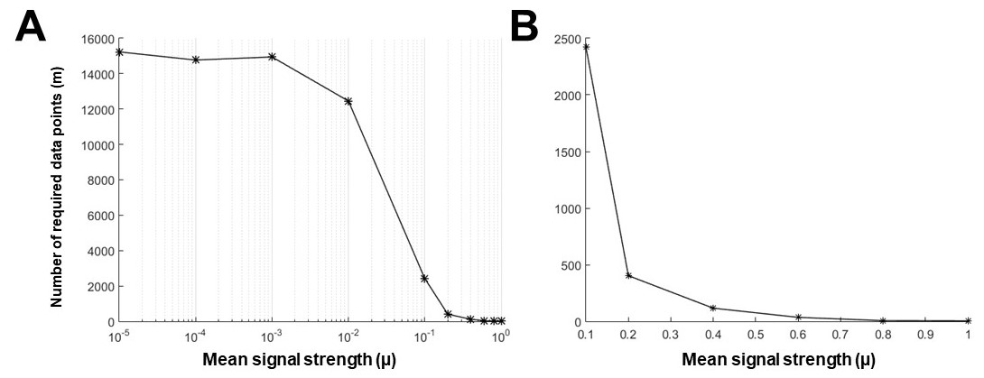
Figure 1: Number of data points required for detection of the non-zero mean $\mu$ with higher criticism.

The results of our simulations explained in §II-F2 are presented in Fig. 2: more data points are needed for the detection of the signal when either its intensity decreases ($\mu$ closer to 0) or it is more sparse ($\varepsilon$ closer to 0).

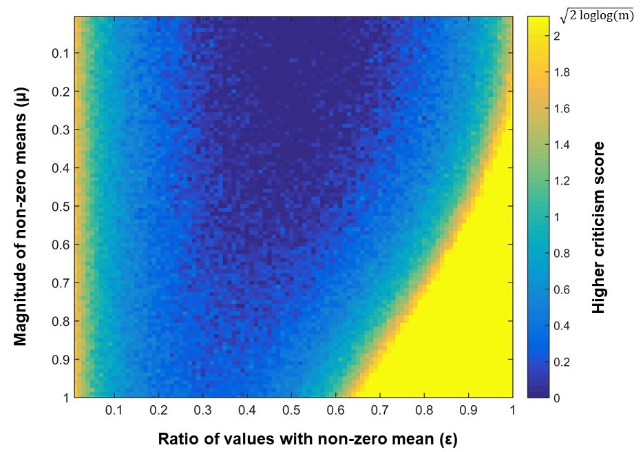
Figure 2: Number of data points required for detection of the weak (represented by $\mu$) and sparse (represented by $\varepsilon$) signal with higher criticism.

III-B Spike detection on electrophysiological data using higher criticism

We explained in §II-D and §II-E the details of our signal detection using HC. The kurtosis of the time series for the electrophysiological data shown in Fig. 3 is equal to 47.58, which indicates that it is far from having a normal distribution. Thus we standardize the time series and find the HC value $HC_{m}$ of the new series to be notably larger than $\sqrt{2\log\log m}$, where $m$ is the length of the time series. The unusually large $HC_{m}$ is compatible with the fact that the kurtosis deviates considerably from 3, and they both assure that we should expect non-normality in the data.

In order to use the algorithm written in §II-D to find the non-normal parts, we need to define a threshold for step 5 of the algorithm. We use different thresholds systematically as explained in §II-E: the silhouette score suggests that we divide the list of the $HC_{m,i}$ to 4 clusters, and we associate a threshold to each cluster by (1). For each threshold, the points that correspond to the $i$ such that $HC_{m,i}$ is larger than than the chosen threshold allow us to localize to the source of non-normality in the data. When we plot these points along with the points that are within 50 time steps away from them, while flattening the remaining points to 0, we detect the signals (large field deflections) of electrophysiological time series, as shown in Fig. 3. That is, Fig. 3A shows the detection with the smallest threshold, where all and only the true signals are detected, with the ability of the method in recognizing two nearby large field deflections demonstrated. Fig. 3B, C, D respectively show the similar detection performed respectively with the 2nd, 3rd and 4th smallest thresholds. It is striking that as the threshold is changed with relatively big jumps, different but only large field deflections are detected, hence a sorting method for neuronal signals based on their statistical properties.

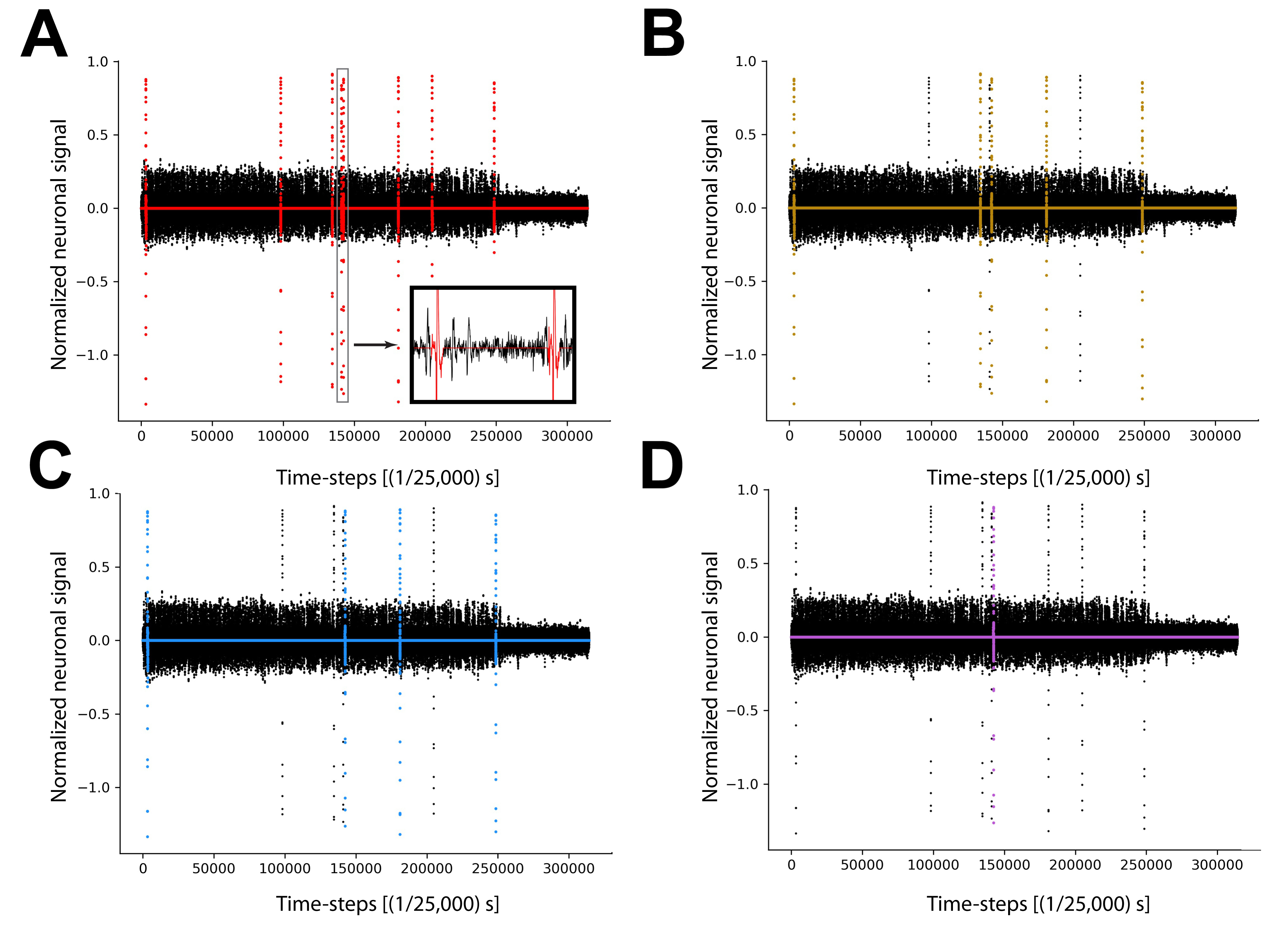
Figure 3: Neuronal signals (large field deflections) detected and sorted with higher criticism.

References

- [1] B. Efron. Large-scale simultaneous hypothesis testing: the choice of a null hypothesis. J. Amer. Statist. Assoc., 99(465):96–104, 2004.
- [2] B. Efron. Large-scale inference, volume 1 of Institute of Mathematical Statistics (IMS) Monographs. Cambridge University Press, Cambridge, 2010. Empirical Bayes methods for estimation, testing, and prediction.
- [3] D. Donoho and J. Jin. Higher criticism thresholding: Optimal feature selection when useful features are rare and weak. Proceedings of the National Academy of Sciences, 105(39):14790–14795, 2008.
- [4] D. Donoho and J. Jin. Higher criticism for large-scale inference, especially for rare and weak effects. Statist. Sci., 30(1):1–25, 2015.
- [5] S. Holmes. Statistical proof? The problem of irreproducibility. Bull. Amer. Math. Soc. (N.S.), 55(1):31–55, 2018.
- [6] L. Cayon, J. Jin, and A. Treaster. Higher criticism statistic: detecting and identifying non-gaussianity in the wmap first-year data. Monthly Notices of the Royal Astronomical Society, 362(3):826–832, 2005.
- [7] E. Parkhomenko, D. Tritchler, M. Lemire, P. Hu, and J. Beyene. Using a higher criticism statistic to detect modest effects in a genome-wide study of rheumatoid arthritis. 3 Suppl 7:S40, 12 2009.
- [8] R. Wehrens and P. Franceschi. Thresholding for biomarker selection in multivariate data using higher criticism. Mol. BioSyst., 8:2339–2346, 2012.
- [9] E. N. Brown, R. E. Kass, and P. P. Mitra. Multiple neural spike train data analysis: state-of-the-art and future challenges. Nature Neuroscience, 7:456 EP –, 04 2004.
- [10] A. H. Barnett, J. F. Magland, and L. F. Greengard. Validation of neural spike sorting algorithms without ground-truth information. Journal of Neuroscience Methods, 264:65 – 77, 2016.
- [11] J. E. Chung, J. F. Magland, A. H. Barnett, V. M. Tolosa, A. C. Tooker, K. Y. Lee, K. G. Shah, S. H. Felix, L. M. Frank, and L. F. Greengard. A fully automated approach to spike sorting. Neuron, 95(6):1381–1394.e6, 2019/01/31 2017.
- [12] J. W. Tukey. The collected works of John W. Tukey. Vol. VIII. Chapman & Hall, New York, 1994. Multiple comparisons: 1948–1983, With a preface by William S. Cleveland, With a biography by Frederick Mosteller, Edited and with an introduction and comments by Henry I. Braun.
- [13] D. Donoho and J. Jin. Higher criticism for detecting sparse heterogeneous mixtures. Ann. Statist., 32(3):962–994, 2004.