Cluster, classify, regress: a general method for learning discontinuous functions

Abstract.

This paper presents a method for solving the supervised learning problem in which the output is highly nonlinear and discontinuous. It is proposed to solve this problem in three stages: (i) cluster the pairs of input-output data points, resulting in a label for each point; (ii) classify the data, where the corresponding label is the output; and finally (iii) perform one separate regression for each class, where the training data corresponds to the subset of the original input-output pairs which have that label according to the classifier. It has not yet been proposed to combine these 3 fundamental building blocks of machine learning in this simple and powerful fashion. This can be viewed as a form of deep learning, where any of the intermediate layers can itself be deep. The utility and robustness of the methodology is illustrated on some toy problems, including one example problem arising from simulation of plasma fusion in a tokamak.

1. Introduction and motivation

Modern times have seen an explosion of available data. This largely originated from the internet, although improved abilities to capture and store data have lead to similar data deluge phenomena in science and engineering applications. Machine learning technology has recently achieved a level of maturity where it is of increasing interest to adapt and apply the fundamental algorithms to problems in science and engineering. However, aside from the big data aspect, the nature of the problems which arise in science are often fundamentally different in character from the problems for which standard machine learning technology was developed. For example, many problems which arise in science and engineering involve highly nonlinear and/or discontinuous functions over high-dimensional parameter spaces [14, 26, 23]. The term “high-dimensional” has different meanings in different contexts, but for the present work it will mean $\gtrsim 10$.

The fantasy of the domain scientist or engineer is that there is a magical black box in which he can dump his data, and out of which will appear a miraculous machine capable of reproducing the results, to suitable accuracy, of his experiments or code which had been months or even generations in development. Indeed, sometimes this is possible with traditional existing methodology. This problem has been studied for a long time in the approximation theory and statistics literature, where it may be referred to as a surrogate or an emulator [31, 10]. The classical problems of machine learning are typically either of classification or regression type. Highly nonlinear and discontinuous functions are something in between, and their reconstruction has been the focus of much existing work in the literature [12, 1, 35, 15, 3, 2, 29, 19], but it is still an active area [5, 17, 37, 24, 11]. In the present work, we propose a simple general framework which can be utilized to solve such problems, using as components the arsenal of available machine learning algorithms [25, 6, 13, 30, 16].

The paper will be organized as follows. In Section 2, the mathematical problem and algorithm will be presented. Section 3 describes an adaptive active learning extension to the current algorithm. The approach is capable of either selecting an opimal subset of training data among an existing set of labeled data, or adaptively selecting training data to label from the domain of all possible (unlabeled) data. Section 4 will feature some numerical illustrations. Finally Section 5 will conclude and discuss some extensions of the present work.

2. Mathematical Setup and Algorithm

The point of departure is a set of labeled training data $\{(x_{i},y_{i})\}_{i=1}^{N}$, where $(x_{i},y_{i})\in\mathcal{X}\times\mathcal{Y}$ are assumed to correspond to input and output of some model

$$y_{i}\approx f(x_{i})\,,$$

and are otherwise considered independent. In other words, we want to do supervised learning. It is furthermore assumed that the model $f:\mathcal{X}\rightarrow\mathcal{Y}$ is highly irregular, including sharp features arising from strong nonlinearities, and most notably including discontinuities. The output space is taken as $\mathcal{Y}=\mathbb{R}$ for simplicity. The important point is that it is continuous. The results can be easily generalized to vector valued outputs. We will also assume $\mathcal{X}=\mathbb{R}^{d}$, although this can also be relaxed. If the data are exact, one can utilize interpolation or projection methods [9, 36], which are generally outside the repertoire of machine learning. However, even in the case of exact data, these methods can be particularly sensitive to the choice of input data points used in the approximation, and can yield poor results. Ordinarily one would look to regression methods in this context, since the output space is continuous. Regression methods handle noisy data elegantly, and are also more robust to the peculiarities of the input data. However, typically regression methods will fail miserably when $f$ has discontinuities (as will interpolation and projection methods). It is therefore natural to attempt to partition the domain according to the discontinuities, and then perform piecewise regression on the continuous components. This strategy has been proposed before in the literature [12, 1, 35, 15, 17, 11, 37]. However, a point which remains unclear is how to identify the continuous components, or equivalently the discontinuous hyper-surfaces, and importantly how to do so without relying on any grid of the input space. Here we propose to use a clustering algorithm to label the input-output training data pairs, coupled with a classification algorithm to label new inputs. To be precise the full method in generality is as follows.

(I) Cluster. First seek a label function which clusters with the training input-output pairs as its inputs

(1) $$\lambda:\mathcal{X}\times\mathcal{Y}\rightarrow\mathcal{L}:=\{1,\dots,L\}\,.$$

The label function typically minimizes an objective function of the form

(2) $$\Phi_{\rm clust}(\lambda)=\sum_{l=1}^{L}\sum_{i\in S_{l}}\ell_{l}(x_{i},y_{i})\,,$$

where $S_{l}=\{(x_{i},y_{i});\lambda(x_{i},y_{i})=l\}$, and $\ell_{l}$ is some loss function associated to cluster $l$. For example, letting $z_{i}=(x_{i},y_{i})$, $\ell_{l}=|z_{i}-\mu_{l}|^{2}$, and $\mu_{l}=\frac{1}{|S_{l}|}\sum_{i\in S_{l}}z_{i}$, where $|\cdot|$ denotes the Euclidean norm for points and counting norm for sets, we have $K-$means clustering. Choosing $L$, for example using the elbow method, completes the clustering phase of the algorithm [6, 13].

(II) Classify. Letting $l_{i}=\lambda(x_{i},y_{i})$, we now have an expanded set of training data $\{(x_{i},y_{i},l_{i})\}_{i=1}^{N}$. The classification phase proceeds to find a function which appropriately labels the inputs according to the labels identified in the cluster phase:

(3) $$f_{c}:\mathcal{X}\rightarrow\mathcal{L}\,.$$

The classifier could be non-parametric or parametric, but the important point is that for each $x\in\mathcal{X}$ it provides an estimate $f_{c}:x\mapsto f(x)\in\mathcal{L}$ such that $f_{c}(x_{i})=l_{i}$ for the majority of the data. This is crucial for the ultimate fidelity of the prediction. Note that the output data $\{y_{i}\}$ is ignored in this phase. The classification function minimizes

(4) $$\Phi_{\rm class}(f_{c})=\sum_{i=1}^{N}\phi_{c}(l_{i},f_{c}(x_{i}))\,,$$

where $\phi_{c}:\mathcal{L}\times\mathcal{L}\rightarrow\mathbb{R}_{+}$ is small if $f_{c}(x_{i})=l_{i}$ and otherwise is not. For example, we can choose $f_{c}(x)={\rm argmax}_{l\in\mathcal{L}}g_{l}(x)$, where $g_{l}(x)>0$, $\sum_{l=1}^{L}g_{l}(x)=1$ is a soft classifier, and $\phi_{c}(l,f_{c}(x))=-\log(g_{l}(x))$ [6, 13, 25], corresponding to cross-entropic loss.

(III) Regress. The final phase of approximation is to find a function which appropriately identifies the original output given the input and the label

(5) $$f_{r}:\mathcal{X}\times\mathcal{L}\rightarrow\mathcal{Y}\,.$$

The regressor could be non-parametric or parametric, but the important point is that for each $(x,l)\in\mathcal{X}\times\mathcal{L}$ it provides an estimate $f_{r}:(x,l)\mapsto f_{r}(x,l)\in\mathcal{Y}$ such that now $f_{r}(x,f_{c}(x))\approx y$ for both training data and test data. If successful then we can expect good reconstruction error for this ultimate predictor

(6) $$f:\mathcal{X}\rightarrow\mathcal{Y}\,,$$

where $f(\cdot)=f_{r}(\cdot,f_{c}(\cdot))$. The regression function can be found by minimizing

(7) $$\Phi_{r}(f_{r})=\sum_{i=1}^{N}\phi_{r}(y_{i},f_{r}(x_{i},f_{c}(x_{i})))\,,$$

where $\phi_{r}:\mathcal{Y}\times\mathcal{Y}\rightarrow\mathbb{R}_{+}$ minimized when $f_{r}(x_{i},f_{c}(x_{i}))=y_{i}$ . In this case we can choose $\phi_{r}(y,f_{r}(x,f_{c}(x)))=|y-f_{r}(x,f_{c}(x))|^{2}$, [6, 13]. Note that it is computationally more expedient to partition the data into $C_{l}=\{i;f_{c}(x_{i})=l\}$, for $l=1,\dots,L$, and then perform $L$ separate regressions (which can also be done in parallel)

(8) $$\Phi_{r}^{l}(f_{r}(\cdot,l))=\sum_{i\in C_{l}}\phi_{r}(y_{i},f_{r}(x_{i},l))\,.$$

Remark 2.1.

A practical consideration with the proposed methodology is the relative scaling of the data in $x=(x^{1},\dots,x^{d})\in\mathbb{R}^{d}$ and $y\in\mathbb{R}$. We have $|(x,y)-(x^{\prime},y^{\prime})|^{2}=(y-y^{\prime})^{2}+|x-x^{\prime}|^{2}$. In particular, notice that if the range is a small fraction of the size of the domain, then even large discontinuities in the output may not be revealed in the clustering. Therefore, it is recommended for the clustering to scale as follows

(9) $$\tilde{x}^{j} = (x^{j}-{\rm min}_{i\in\{1,\dots,N\}}x_{i}^{j})/|(x^{j}-{\rm min}_{i\in\{1,\dots,N\}}x_{i}^{j})|\,\quad{\rm for}\quad j=1,\dots,d,$$

(10) $$\tilde{y} = C(y-{\rm min}_{i\in\{1,\dots,N\}}y)/|(y-{\rm min}_{i\in\{1,\dots,N\}}y)|\,,$$

for $C>1$. In particular, it is recommended to choose $C=10d$, where $d={\rm dim}x$. One could also use some other type of standardization, e.g. subtracting the mean and dividing by the standard deviation. For the regression it is recommended to set $C=1$ above, as smaller variations in $y$ are easier to deal with for regression.

Remark 2.2.

A critique of this method is that it re-uses the data in each phase. We note that there is a Bayesian formulation, which will be considered in a future work. Let $D=\{(x_{i},y_{i})\}_{i=1}^{N}$, assume we have parametric models for the classifier $g_{l}(\cdot;\theta_{c})=g_{l}(\cdot;\theta_{c}^{l})$, and the regressor $f_{r}(\cdot,l;\theta_{r}^{l})$, for $l=1,\dots,L$, where $\theta_{c}=(\theta_{c}^{1},\dots,\theta_{c}^{L})$ and $\theta_{r}=(\theta_{r}^{1},\dots,\theta_{r}^{L})$ index the parameters corresponding to each class, and let $\theta=(\theta_{c},\theta_{r})$. Then the posterior density has the form

$$\pi(\theta,l|D)\propto\prod_{i=1}^{N}\pi(y_{i}|x_{i},\theta_{r},l)\pi(l|x_{i},\theta_{c})\pi(\theta_{r})\pi(\theta_{c})\,,$$

where, for example,

$$\pi(y_{i}|x_{i},\theta_{r},l)\propto\exp(-\frac{1}{2}|y_{i}-f_{r}(x_{i},l;\theta_{r}^{l})|^{2})\,,$$

and

$$\pi(l|x_{i},\theta_{c})=g_{l}(x_{i};\theta_{c})\,.$$

In this case we may take for example

$$g_{l}(x;\theta_{c})=\frac{\exp(h_{l}(x;\theta_{c}^{l}))}{\sum_{l=1}^{L}\exp(h_{l}(x;\theta_{c}^{l}))}\,,$$

where $h_{l}(\cdot;\theta_{c}^{l})$ are some standard parametric regressors.

It is important to note that fully Bayesian solutions, while elegant, clean, and complete with Occam’s razor, are also very expensive. This example is grid-free, at least, and this feature will be desirable for high-dimensional problems of the type considered here. It will be interesting to compare this method to grid-based Bayesian approaches such as [11, 24]. If the regressors are defined in terms of grids, for example $\theta_{r}^{l}$ are the coefficients of expansion in piecewise linear finite element nodal basis functions [38], then there are similarities between the methods.

Remark 2.3.

Another important critique is that the method will struggle if there are discontinuities which appear or vanish within the domain, for example the product of a heaviside and a vanishing function, as the phase (I) clustering will fail in this case. However, in practice, we have found that the method is able to handle such cases with a very large number of clusters, i.e. much greater than the number of continuous components.

3. Active learning extension

Here it is described how to embed the algorithm above into an active learning strategy [32]. First, observe that the fundamental steps above are (I-II), as a continuous approximation (III) of a function with a discontinuity will always be a poor approximation. Indeed the error in such approximations is typically concentrated around the discontinuities. For this reason, it is preferable to choose a soft-classifier (or probabilistic classifier) [25], even if the ultimate classification is taken as a thresholding of such continuous function, as described above in (II) for multiclass logistic regression. Suppose we have a soft classifier $\{g_{l}(x)\}_{l\in\mathcal{L}}$, $\sum_{l\in\mathcal{L}}g_{l}(x)=1$, such that $g_{l}(x)$ represents the probability that point $x$ is in class $l$, and our classification is given by $f_{c}(x)={\rm argmax}_{l\in\mathcal{L}}g_{l}(x)$. Suppose we have some initial set of $N_{\rm init}$ training data points $\mathcal{D}_{\rm init}:=\{x_{-N_{\rm init}+1},x_{-N_{\rm init}+2},\dots,x_{0}\}$.

Active Strategy 1. It is natural to seek, for $n>0$,

(11) $$x_{n}={\rm argmin}_{x\in\mathcal{D}_{n}}{\rm max}_{l\in\mathcal{L}}g_{l}(x)\,,$$

for some appropriate compact domain $\mathcal{D}_{n}\subseteq\mathcal{X}$.

Active Strategy 1a. An extremely simple example would be the case in which $\mathcal{D}_{1}=\mathcal{D}_{\rm init}$ and $\mathcal{D}_{n}=\{x_{1},\dots x_{N_{\rm res}}\}\backslash\mathcal{D}_{n-1}$ is a finite subset of the domain, consisting of $N_{\rm res}$ points which we refer to as the “reservoir”, which may for example be existing labeled points which we are aiming to scrupulously include in our training algorithm.

Active Strategy 1b. Alternatively, we may constrain the algorithm to search only some continuous subset of the possible (currently unlabelled) input data. Here we either need an a priori defined domain, or some sensible way of adapting the domain. If we know the input data of interest lies within some hypercube $\mathcal{D}=\prod_{i=1}^{d}[a_{i},b_{i}]$, then it may be reasonable to choose this as $\mathcal{D}_{n}=\mathcal{D}$. However, one expects that often the data may be concentrated on some manifold within such a hypercube. In that case, the naive strategy just mentioned would lead to many points in the large volume of the parameter space which is uninteresting and will never be queried in practice. An alternative which may be viable in the case that the initial data $\mathcal{D}_{\rm init}$ is suitably rich, and concentrated on the appropriate data manifold, would be to let $\mathcal{D}={\rm conv}\mathcal{D}_{\rm init}$, the convex hull of the initial data set. Note that in this case the training data will always remain in this set.

Active Strategy 2. This strategy operates on the assumption of the latter version of strategy 1b, i.e. that $\mathcal{D}={\rm conv}\mathcal{D}_{\rm init}$ provides suitable coverage of the input domain of interest. Let $\mathcal{D}_{1}=\mathcal{D}_{\rm init}$. Let $\mathcal{N}^{n}_{k}(x)$ denote the $k$ nearest neighbors of $x$ in $\mathcal{D}_{n}$, where $k\geq 1$. Let

$$\mathcal{S}_{n}=\{x\in\mathcal{D}_{n};\exists y\in\mathcal{C}_{n}(x)\}\,,\qquad\mathcal{C}_{n}(x)=\{y\in\mathcal{N}_{k}(x);f_{c}(x)\neq f_{c}(y)\}\,.$$

Now, let the batch of new training data at step $n$, $\mathcal{B}_{n}$, be defined by those points $z^{*}$, one for each $x\in\mathcal{S}_{n}$ and each $y\in\mathcal{C}_{n}(x)$, such that

$$z^{*}={\rm argmin}_{z\in\mathcal{A}}{\rm max}_{l\in\mathcal{L}}g_{l}(z),\quad\mathcal{A}=\{z\in\mathcal{D};z=\lambda x+(1-\lambda)y\}\,.$$

This strategy is prone to degeneration, and so has to be regenerated once in a while, for example with strategy 1b or strategy 3 below. When all $x\in\mathcal{S}_{n}$ and $y\in\mathcal{C}_{n}(x)$ are exhausted, we have $n^{*}\sum_{x\in\mathcal{S}_{n}}|\mathcal{C}_{n}(x)|$ new data points, $\mathcal{D}^{*}$ which are concatenated to the present set $\mathcal{D}_{n+1}=\mathcal{D}_{n}\cup\mathcal{D}^{*}$.

Active Strategy 3. Here we choose some set $\mathcal{A}$ (different from above), for example with any one of the strategies above, and we then choose points $z_{i}(x)\sim Q(x,\cdot)$, for $i=1,\dots,n$, from a Markov kernel $Q$ (i.e. $Q(x,\cdot)$ is a probability distribution for each $x\in\mathcal{X}$), for each $x\in\mathcal{A}$. We could let $Q(x,\cdot)$ be a uniform on the $d-$dimensional hypercube centered at $x$, or a normal centered at $x$. It can be uniform/standard, or the covariance could be determined by the sample covariance of $\mathcal{N}^{n}_{k}(x)$ with a suitably large $k$, in order to stay faithful to the local manifold structure of the data.

Remark 3.1.

Note with strategy 1 that there are likely infinitely many solutions to the optimization problem. Consider binary linear classification, where we choose label $1$ if $g_{1}(x)>1/2$ and label $2$ otherwise, and there is a separating hyperplane if $g_{1}$ is linear. Along the hyperplane we have $g_{1}(x)=1/2$, i.e. there is a linear subspace of dimension $d-1$ which solves the problem (11). This is not a major concern, as we only need one point, and any of these points will equivalently enrich the training set.

Remark 3.2.

We are mostly concerned with the case in which we can label any point, but the labelling itself is the limiting cost. So active strategy 1a may be of limited practical value.

Remark 3.3.

The choice of domain $\mathcal{D}$ is important for strategy 1b. If $\mathcal{D}=\mathcal{X}=\mathbb{R}^{d}$, then the strategy above is likely to seek points outside the convex hull of the existing training data, where nothing is known about the classifier. The danger is that we may not want to know anything about the classifier in that region.

Remark 3.4.

Motivated by the discussion at the beginning of this section, all strategies presented here are based on what is known as uncertainty sampling [32]. Other objectives can be used as well (or none at all, i.e. random sampling), including

1. Entropy sampling: one chooses the point whose class probability has the largest entropy.

2. Margin sampling: one chooses the point for which the difference between the most and second most likely classes is the smallest.

Remark 3.5.

This section is not to be confused with simple adaptive online learning, in which the machine may be embedded within a workflow and queried regularly for some input $x_{\rm new}$. In this case, one would employ a similar but distinct approach. First, evaluate the fitness of the machine for the queried point $x_{\rm new}$. For example, as in (11) we may compute ${\rm max}_{l\in\mathcal{L}}g_{l}(x_{\rm new})$. Then, if the fitness is suitable (in this case the probability of the most likely class being sufficiently close to 1), we proceed with the machine. If the fitness is low, we augment the training set with this new point and refine the machine. In this case, one may venture to decide if the new query point is suitably close to the existing set of training data, and if not then refine within the convex hull as described in strategy 1b or 2 above.

4. Method used and Numerical examples

Clearly there is enormous potential for exploring various configurations of the component algorithms, but since the purpose of this paper is to introduce the method and illustrate its power on some simple examples we choose only some of the most basic component algorithms.

For clustering, K-means clustering [6] is used, as described in Section 2 (I). The standard iterative algorithm is used to optimize the objective function (2). The elbow method is used to determine the value of $L$ [6]. For regression and classification, multi-layered perceptrons (MLPs) are used [6], with a single hidden layer of $100d$ neurons and ReLU$(x)={\rm max}\{0,x\}$ activation function for both. For the multi-classification, the output layer is given by a softmax, with a cross-entropy loss function, as described in Section 2 (II). For regression, the output activation is linear, and the loss function is quadratic, as described in Section 2 (III). A quadratic regularization is used in both cases, with parameter $0.001$. The adaptive stochastic gradient descent solver Adam [21] is used to optimize (4) and the $L$ functions (8). A validation fraction of $0.1$ is employed and the number of iterations are limited by a maximum of $200$. In examples 3 and 4, a random forest method [8] is used, in which $100$ bootstrapped classification or regression decision trees are aggregated [7], where each one involves a subset of only ceil$(d/3)$ input parameters. The scikit learn python package [28] is used for all the basic learning algorithms employed.

4.1. Numerical experiments

In this section several prototype models are considered. First, let $\mathcal{X}=\mathbb{R}$ and consider the simple example $f_{1}(x)=x{\bf 1}_{x\geq 1}$, where

$${\bf 1}_{A}(x)=\left\{\begin{array}[]{cc}1&x\in A\\ 0&{\rm else}\\ \end{array}\right\}\,.$$

The function is plotted in Figure 1 row (a), column (a), along with the prediction results of the final CCR machine output $f_{r}(x;f_{c}(x))$, and the intermediate $f_{c}(x)$. Figure 1 row (a), column (b) shows a scatter plot of the true $f_{1}(x)$ and the CCR machine $f_{r}(x;f_{c}(x))$, illustrating the correlation. Figure 1 row (a), column (d) shows a histogram of $f_{r}(x;f_{c}(x))-y(x)$, illustrating the dissimilarity between the CCR reconstruction and the truth.

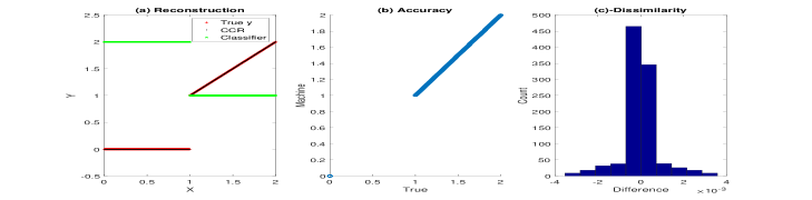
(a) Numerical example 1, $f_{1}$.

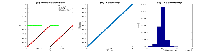
(b) Numerical example 2, $f_{2}$.

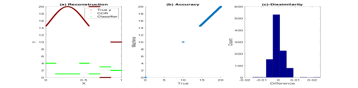
(c) Numerical example 3, $f_{3}$.

Figure 1. Numerical examples 1 (row a), 2 (row b), and 3 (row c). The functions are plotted in columns (a), along with the final CCR machine output $f_{r}(x;f_{c}(x))$, and the intermediate $f_{c}(x)$. Columns (b) show a scatter plot of the true $f(x)$ and the CCR machine $f_{r}(x;f_{c}(x))$, illustrating the correlation. Panel (d) shows a histogram of $f_{r}(x;f_{c}(x))-f(x)$, illustrating the dissimilarity between the CCR reconstruction and the truth.

Notice that the previous example could have been dealt with using a simple clustering of the output values $y\in\mathbb{R}$ alone. Consider the slightly more complicated function $f_{2}(x)=(x+1){\bf 1}_{x<0}+x{\bf 1}_{x\geq 0}$, for $\mathcal{X}=[-1,1]$. Here the $y$-values alone cannot be used for clustering, as they suggest a single cluster is optimal (e.g. using the elbow method would return $L=1$). However, our method of clustering input-output pairs $(x,y)\in\mathbb{R}^{2}$ works here, and elbow returns $L=2$. The method is illustrated on this example in Figure 1, row (b) whose panels are the same as Figure 1a. Note that due to the gross simplicity of the model, if we look for 2 clusters based on $y$ values alone, then we would get something like $y\in[0,0.5]$ and $y\in(0.5,1]$. In other words, we would bypass the issue of the discontinuity, as a single class would not span the discontinuity, and this is the primary requirement in order for the piecewise regression to perform well. This will not hold in general, but it is illustrative of the robustness afforded by choosing extra clusters and extra amplification of $y$.

Note that the first 2 functions can both be reconstructed exactly with relatively simple multilayer perceptrons, provided discontinuous activation functions are utilized. Consider a 3 node hidden layer with $z_{1}={\rm max}\{0,x\}$, $z_{2}={\rm max}\{0,-x\}$, $z_{3}={\bf 1}_{x\geq 0}$, and $z_{4}={\bf 1}_{-x\geq 0}$. Then we have $f_{1}(x)=1+z_{1}-z_{4}$ and $f_{2}(x)=1-z_{2}+z_{1}-z_{3}$. However, it is difficult in general to cook up an architecture which is appropriate for arbitrary high-dimensional functions which have multiple discontinuities along nonlinear hyper-surfaces and highly nonlinear components, as will be introduced in the following examples. On the other hand, CCR is flexible and easy to implement, and its basic components are well-understood. Furthermore, discontinuous activation functions are problematic for gradient-based optimization methods, which are commonly employed.

To illustrate the benefit of CCR with simple MLPs in comparison to alternative regression methods, we compare two direct regression methods on $f_{2}$. The first is an MLP with a single hidden layer of 100 neurons with ReLU activation functions, and a linear output. The second is a deep neural network (DNN) with 3 hidden layers of 200, 420, and 21 neurons each, with ReLU activation functions, and linear output. The results are presented in Figure 2. It is clear that neither of the simple regression methods are able to cleanly recover the discontinuity.

Figure 2. The results of CCR (a), DNN (b), and MLP(c) as applied to numerical example 2 $f_{2}$.

Now we consider slightly more complicated functions, following the recent work [24]. First, consider $\mathcal{X}=[-4,10]$ and

(12) $$f_{3}(x)=\left\{\begin{array}[]{cc}\exp(-x^{2}/20)&x\leq 4\\ 1&4<x\leq 6\\ -1&6<x\leq 8\\ 0&x>8\end{array}\right\}\,.$$

Notice that the range of $f_{3}$ is very small in comparison to the domain $\mathcal{X}$. Therefore this is a prime example where the transformation (9) needs to be utilized. The method is illustrated on this example in Figure 1 row (c), whose panels are the same as the rows above.

The next example is simple the product of the previous, so $\mathcal{X}=[-4,10]^{2}$ and $f_{4}(x)=f_{3}(x_{1})f_{3}(x_{2})$. The method is illustrated on this example in Figure 3. Here the information is the same as Figure 1, but now $f_{4}(x)$ is plotted in panel (a), and $f_{r}(x,f_{c}(x))$ and $f_{c}(x)$ are plotted in panels (b) and (c), respectively. Panel (e) shows a scatter plot of the true $f_{4}(x)$ and the CCR machine $f_{r}(x;f_{c}(x))$, illustrating the correlation. Panel (f) shows a histogram of $f_{r}(x;f_{c}(x))-y(x)$, illustrating the dissimilarity between the CCR reconstruction and the truth. Panel (g) shows the elbow plot. Notice that there is no clear elbow. One might choose $L=4$ clusters, but this is not sufficient to avoid any cluster spanning a discontinuity. From a visual inspection, $L=7$ is the minimum number of continuous components, if we group components which meet at a point. In this case, sometimes we get a good set of clusters, but sometimes some clusters span a discontinuity. If we let these each correspond to 2 distinct components, then $L=10$, which we find is sufficient to ensure no single cluster spans a discontinuity. This is another illustration of the robustness of choosing extra clusters. Interestingly, the clusters we find do not correspond to the continuous components at all, but rather (as in previous examples 2-3) partition the function primarily based on $y$-value contour level set intervals, crucially none of which span a discontinuity.

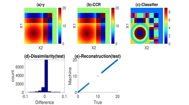
Figure 3. Numerical example 4. $f_{4}(x)$ is plotted in panel (a), and $f_{r}(x,f_{c}(x))$ and $f_{c}(x)$ are plotted in panels (b) and (c), respectively. Panel (e) shows a scatter plot of the true $y(x)$ and the CCR machine $f_{r}(x;f_{c}(x))$, illustrating the correlation. Panel (d) shows a histogram of $f_{r}(x;f_{c}(x))-y(x)$, illustrating the dissimilarity between the CCR reconstruction and the truth.

4.2. Critical gradient model for tokamaks

A tokamak is a device which uses magnetic fields to confine hot plasma in the shape of a torus. It is the leading candidate for production of controlled thermonuclear power, for use in a prospective future fusion reactor [18].

One dimensional radial transport modeling [27] using theory-based models such as GLF23 [34], MMM95 [4], and TGLF [33] plays an essential role in interpreting experimental data and guiding new experiments for magnetically confined plasmas in tokamaks. Turbulent transport resulting from micro-instabilities have a strong nonlinear dependency on the temperature and density gradients. One of the key characteristics is a sharp increase of turbulent flux as the gradient of temperature increases beyond a certain critical value. This leads to a highly nonlinear and discontinuous function of the inputs.

Here we consider an analytic stiff transport model that describes turbulent ion energy transport in tokamak plasmas [20]:

(13) $$\chi=S(RT^{\prime}/T-(RT^{\prime}/T)_{\rm crit})^{\alpha}H\left(\left|\frac{(RT^{\prime}/T)}{(RT^{\prime}/T)_{\rm crit}}\right|-1\right)\,,$$

where $\chi$ is ion thermal diffusivity, $H(\cdot)$ is the Heaviside function, $R$ is the major radius, and $T^{\prime}$ is the radial derivative of ion temperature. The normalized critical gradient $(RT^{\prime}/T)_{\rm crit}$ of ion temperature is calculated using IFS/PPPL model [22], which is a nonlinear function of electron density ($n_{e}$), electron and ion temperatures ($T_{e},T$), safety factor ($q$), magnetic shear ($\hat{s}$), effective charge ($Z_{\rm eff}$) and the normalized gradient of ion temperature $(RT^{\prime}/T)$ and density $(Rn^{\prime}/n)$. It is assumed that $S=1$ and $\alpha=1$. Considering $(T,T^{\prime})$ and $(n,n^{\prime})$ as two input parameters each, this gives a total of 10 inputs $x\in\mathbb{R}^{10}$. The output (13) is $y\in\mathbb{R}_{+}$. Basic primitive model inputs are chosen uniformly at random from a hypercube $\omega\in[0,1]^{17}$, which then give rise to realistic inputs $x\in\mathbb{R}^{10}$, which concentrate on a manifold in the ambient space. See [22] for details of the model, and Figure 4 (b) for visualization of the input distribution histogram. It is difficult to visualize a function over $\mathbb{R}^{10}$, so we plot some slices in Figure 4 (a) in order to get a sense of it. This is now explained. Let $m=\mathbb{E}(x)$, where the expectation is with respect to the input distribution. For $i=4$ and $j=6,9,10$ (in rows 1, 2, 3, respectively), $\chi(x)$ is plotted as $x$ varies over a $2d$ grid $(m_{1},\dots,m_{j-1},x_{j},m_{j+1},\dots m_{i-1},x_{i},m_{i+1},\dots,m_{10})$.

The CCR method is illustrated on this example in Figure 5. Here $N_{\rm train}=300000$ training data points are used, and $N_{\rm test}=500$ test data points.

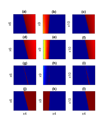
(a) Some slices of $f_{5}=\chi$.

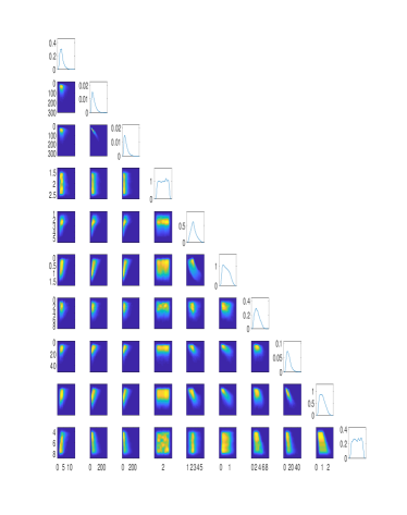
(b) Input distribution marginals.

Figure 4. Numerical example 5: subfigure (a) shows some two variable slices of the true function $\chi$ (a-c), the CCR machine output $f_{r}(x;f_{c}(x))$ (d-f), the absolute difference $|\chi-f_{r}(x;f_{c}(x))|$ (g-i), and the intermediate $f_{c}(x)$ (j-l), with remaining inputs set to the mean $\mathbb{E}(x_{\backslash ij})$, where $x_{\backslash ij}=(m_{1},\dots,m_{j-1},m_{j+1},\dots m_{i-1},m_{i+1},\dots,m_{10})$. Subfigure (b) shows the input data distribution marginals.

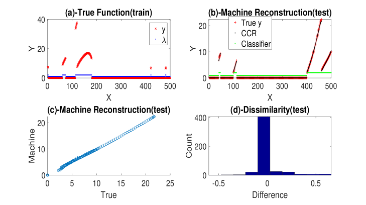
Figure 5. Numerical example 5. The first 500 (random) training data output values are plotted in Panel (a), along with the clustering values of the training data. Panel (b) shows prediction results on test data: the final CCR machine output $f_{r}(x;f_{c}(x))$, the true $y(x)$, and the intermediate $f_{c}(x)$. Panel (c) shows a scatter plot of the true $y(x)$ and the CCR machine $f_{r}(x;f_{c}(x))$, illustrating the correlation. Panel (d) shows a histogram of $f_{r}(x;f_{c}(x))-y(x)$, illustrating the dissimilarity between the CCR reconstruction and the truth.

4.3. Accuracy and active learning extensions

Accuracy	Example 1	Example 2	Example 3	Example 4	Example 5
L2 (%)	0.9934	0.9961	0.9964	0.9978	0.9825
R2 (%)	0.9978	0.9967	0.9987	0.9983	0.9845

Table 1. L2 and R2 comparison for the 5 numerical examples.

The accuracy of the methods on test data is presented in Table 1. In particular,

(14) $$L2=1-\sqrt{\frac{\sum_{i=1}^{N}|f_{r}(x_{i};f_{c}(x_{i}))-y_{i}|^{2}}{\sum_{i=1}^{N}|y_{i}|^{2}}}\,,$$

and

(15) $$R2=1-\frac{\sum_{i=1}^{N}|f_{r}(x_{i};f_{c}(x_{i}))-y_{i}|^{2}}{\sum_{i=1}^{N}|y_{i}-\bar{y}|^{2}}\,,$$

where $\bar{y}=\frac{1}{N}\sum_{i=1}^{N}y_{i}$. For example 5, the data used to compute the error is out-of-sample testing data. For the grid-based examples, it is the training data.

	Active	Passive
Error	0.1	0.15
$N$	150	1000

Table 2. Error attainment with set of sample points for active learning with Example 2 and strategy 1a: $N_{\rm res}=1000$ and all points are used for passive learning, while only $n=150$ points are used for active.

Table 2 illustrates active learning with active strategy 1a from Section 3.

5. Discussion

In this work we present a simple general framework for using the existing arsenal of fundamental machine learning tools in order to solve the challenging problem of reconstructing a surrogate model, or machine, for approximating highly nonlinear and discontinuous functions over high dimensional spaces. We have illustrated the power and accuracy of the method on various examples. It is notable that the method admits a huge amount of flexibility, as any combination of clustering, classification, and regression models will work. It can also be wrapped around existing deep learning architectures, which typically already combine elements of the latter 2. Therefore, it is reasonable to call this super deep learning. The cost of the regression stage may be high if there are many classes/clusters, since there is one regression per class, but this stage is also embarrassingly parallel.

Acknowledgements: This work is supported by the U.S. Department of Energy, Office of Science, Office of Advanced Scientific Computing Research (ASCR) Scientific Discovery through Advanced Computing (SciDAC) project on Advanced Tokamak Modelling (AToM), under field work proposal number ERKJ123.

References

- [1] David Adalsteinsson and James A Sethian. A fast level set method for propagating interfaces. Journal of computational physics, 118(2):269–277, 1995.
- [2] Rick Archibald, Anne Gelb, Rishu Saxena, and Dongbin Xiu. Discontinuity detection in multivariate space for stochastic simulations. Journal of Computational Physics, 228(7):2676–2689, 2009.
- [3] Rick Archibald, Anne Gelb, and Jungho Yoon. Polynomial fitting for edge detection in irregularly sampled signals and images. SIAM journal on numerical analysis, 43(1):259–279, 2005.
- [4] Glenn Bateman, Arnold H Kritz, Jon E Kinsey, Aaron J Redd, and Jan Weiland. Predicting temperature and density profiles in tokamaks. Physics of Plasmas, 5(5):1793–1799, 1998.
- [5] Dmitry Batenkov. Complete algebraic reconstruction of piecewise-smooth functions from fourier data. Mathematics of Computation, 84(295):2329–2350, 2015.
- [6] Christopher M Bishop. Pattern recognition and machine learning. springer, 2006.
- [7] Leo Breiman. Bagging predictors. Machine learning, 24(2):123–140, 1996.
- [8] Leo Breiman. Random forests. Machine learning, 45(1):5–32, 2001.
- [9] Hans-Joachim Bungartz and Michael Griebel. Sparse grids. Acta numerica, 13:147–269, 2004.
- [10] Stefano Conti and Anthony O?Hagan. Bayesian emulation of complex multi-output and dynamic computer models. Journal of statistical planning and inference, 140(3):640–651, 2010.
- [11] Matthew M Dunlop, Marco A Iglesias, and Andrew M Stuart. Hierarchical bayesian level set inversion. Statistics and Computing, 27(6):1555–1584, 2017.
- [12] Knut S Eckhoff. Accurate reconstructions of functions of finite regularity from truncated fourier series expansions. Mathematics of Computation, 64(210):671–690, 1995.
- [13] Jerome Friedman, Trevor Hastie, and Robert Tibshirani. The elements of statistical learning, volume 1. Springer series in statistics New York, 2001.
- [14] Timothy S Gardner, Charles R Cantor, and James J Collins. Construction of a genetic toggle switch in escherichia coli. Nature, 403(6767):339, 2000.
- [15] Anne Gelb and Eitan Tadmor. Spectral reconstruction of piecewise smooth functions from their discrete data. ESAIM: Mathematical Modelling and Numerical Analysis, 36(2):155–175, 2002.
- [16] Ian Goodfellow, Yoshua Bengio, and Aaron Courville. Deep learning. MIT press, 2016.
- [17] Alex Gorodetsky and Youssef Marzouk. Efficient localization of discontinuities in complex computational simulations. SIAM Journal on Scientific Computing, 36(6):A2584–A2610, 2014.
- [18] John Greenwald. Major next steps for fusion energy based on the spherical tokamak design, 2016.
- [19] John D Jakeman, Richard Archibald, and Dongbin Xiu. Characterization of discontinuities in high-dimensional stochastic problems on adaptive sparse grids. Journal of Computational Physics, 230(10):3977–3997, 2011.
- [20] G Janeschitz, GW Pacher, O Zolotukhin, G Pereverzev, HD Pacher, Y Igitkhanov, G Strohmeyer, and M Sugihara. A 1-d predictive model for energy and particle transport in h-mode. Plasma physics and controlled fusion, 44(5A):A459, 2002.
- [21] Diederik P Kingma and Jimmy Ba. Adam: A method for stochastic optimization. arXiv preprint arXiv:1412.6980, 2014.
- [22] M Kotschenreuther, W Dorland, MA Beer, and GW Hammett. Quantitative predictions of tokamak energy confinement from first-principles simulations with kinetic effects. Physics of Plasmas, 2(6):2381–2389, 1995.
- [23] Orso Meneghini, Sterling P Smith, Philip B Snyder, Gary M Staebler, Jeffrey Candy, E Belli, L Lao, Mark Kostuk, T Luce, Teobaldo Luda, et al. Self-consistent core-pedestal transport simulations with neural network accelerated models. Nuclear Fusion, 57(8):086034, 2017.
- [24] Karla Monterrubio-Gómez, Lassi Roininen, Sara Wade, Theo Damoulas, and Mark Girolami. Posterior inference for sparse hierarchical non-stationary models. arXiv preprint arXiv:1804.01431, 2018.
- [25] Kevin P Murphy. Machine Learning: A Probabilistic Perspective. The MIT Press, 2012.
- [26] Habib N Najm, Bert J Debusschere, Youssef M Marzouk, Steve Widmer, and OP Le Maître. Uncertainty quantification in chemical systems. International journal for numerical methods in engineering, 80(6-7):789–814, 2009.
- [27] Jin Myung Park, Masanori Murakami, HE St John, Lang L Lao, MS Chu, and Ronald Prater. An efficient transport solver for tokamak plasmas. Computer Physics Communications, 214:1–5, 2017.
- [28] Fabian Pedregosa, Gaël Varoquaux, Alexandre Gramfort, Vincent Michel, Bertrand Thirion, Olivier Grisel, Mathieu Blondel, Peter Prettenhofer, Ron Weiss, Vincent Dubourg, et al. Scikit-learn: Machine learning in python. Journal of machine learning research, 12(Oct):2825–2830, 2011.
- [29] Dirk Pflüger, Benjamin Peherstorfer, and Hans-Joachim Bungartz. Spatially adaptive sparse grids for high-dimensional data-driven problems. Journal of Complexity, 26(5):508–522, 2010.
- [30] Carl Rasmussen and Chris Williams. Gaussian processes for machine learning. Gaussian Processes for Machine Learning, 2006.
- [31] Jerome Sacks, William J Welch, Toby J Mitchell, and Henry P Wynn. Design and analysis of computer experiments. Statistical science, pages 409–423, 1989.
- [32] Burr Settles. Active learning literature survey. Technical report, University of Wisconsin-Madison Department of Computer Sciences, 2009.
- [33] GM Staebler, JE Kinsey, and RE Waltz. A theory-based transport model with comprehensive physics. Physics of Plasmas, 14(5):055909, 2007.
- [34] RE Waltz, GM Staebler, W Dorland, GW Hammett, Mike Kotschenreuther, and JA Konings. A gyro-landau-fluid transport model. Physics of Plasmas, 4(7):2482–2496, 1997.
- [35] Michael Yu Wang, Xiaoming Wang, and Dongming Guo. A level set method for structural topology optimization. Computer methods in applied mechanics and engineering, 192(1-2):227–246, 2003.
- [36] Dongbin Xiu. Numerical methods for stochastic computations: a spectral method approach. Princeton university press, 2010.
- [37] Guannan Zhang, Clayton G Webster, Max Gunzburger, and John Burkardt. Hyperspherical sparse approximation techniques for high-dimensional discontinuity detection. SIAM review, 58(3):517–551, 2016.
- [38] Olgierd Cecil Zienkiewicz, Robert Leroy Taylor, Perumal Nithiarasu, and JZ Zhu. The finite element method, volume 3. McGraw-hill London, 1977.