Nearly Markovian maps and entanglement-based bound on corresponding non-Markovianity

Abstract

We identify a set of dynamical maps of open quantum system, and refer to them as “$\epsilon$-Markovian” maps. It is constituted of maps which, in a higher dimensional system-environment Hilbert space, possibly violate Born approximation but only a “little”. We characterize the “$\epsilon$-nonmarkovianity” of a general dynamical map by the minimum distance of that map from the set of $\epsilon$-Markovian maps. We analytically derive an inequality which gives a bound on the $\epsilon$-nonmarkovianity of the dynamical map, in terms of an entanglement-like resource generated between the system and its “immediate” environment. In the special case of a vanishing $\epsilon$, this inequality gives a relation between the $\epsilon$-nonmarkovianity of the reduced dynamical map on the system and the entanglement generated between the system and its immediate environment. We numerically investigate the behavior of the similar distant based measures of non-Markovianity for classes of amplitude damping and phase damping channels.

I Introduction

The study of open quantum systems is of fundamental importance in several areas, including the field of quantum information. In an ideal scenario, the evolution of a closed quantum system is described by a unitary operation and is mathematically described by the Schrödinger’s equation. But in the real world, a system is never perfectly isolated. The interaction with the environment gives rise to non-unitary evolution of the quantum system which causes dissipation of energy and loss of coherence. In arguably the simplest case, the mathematical model of the evolution of an open system is derived using a number of assumptions, which, collectively, has been christened as the “Markovian” approximation petru . A principal underlying assumption is that the coupling between the system and the environment is weak, so that the environmental excitations decay in a time much shorter than the time it takes for the system to evolve from initial state. For such a process, the information that flows from the system to the environment can never come back to the system, i.e. the system does not have a memory. In contrast to that, if the interaction between system and environment is such that the information flow can happen both ways, the system is said to have memory-effects. Several variations of this conceptualization of quantum Markovianity and non-Markovianity exists in the literature for evolution of open quantum systems petru ; other-than-Petru ; TnaDbaro ; other1 .

Over the years, a number of non-Markovianity measures have been proposed. This includes a measure that identifies non-Markovianity by studying the time-dynamics of entanglement between the system and an auxiliary system RHP . A Markovian evolution causes monotonic decrease of the entanglement, whereas a non-Markovian evolution may give rise to consecutive decay and revival of the entanglement between system and auxiliary system. This behavior of entanglement can be captured in the divisibility property of the dynamical map of the reduced system. Using the concept of divisibility of dynamical maps wolf , Rivas et al. RHP formulated a necessary and sufficient criterion to detect non-Markovianity when the exact form of the dynamical map of the reduced system is known. Further studies in this direction include odvut . There are several works that look for manifestation of non-Markovianity in the non-monotonic behaviour of a number of other quantum-mechanical properties of a system, e.g. flow of quantum Fisher information lu , fidelity difference usha , quantum mutual information luo , volume of accessible states of a system lorenzo , accessible information fanchini , total entropy production salimi , quantum interferometric power dhar , coherence chanda , etc. Another class of measures, proposed by Breuer et al. BLP (see also rattir-baroTar-par-Kolkata-shasan-kare-charjan-jubak ), associates the distinguishability of quantum states with the non-Markovian behavior of their evolution. A backflow of information from the environment to the system possibly increases the distinguishability, whereas in case of Markovian evolution, the one-way information flow from the system to the surroundings results in monotonic decrease of the distinguishability of the quantum states BLP1 ; MLBMP ; AFPP . However, there are instances when these different non-Markovianity measures are not in agreement with each other. Specific examples show that the evolution of an open quantum system can be Markovian according to BLP but the corresponding dynamical map is indivisible and hence the evolution is non-Markovian according to RHP haikka ; CMR . Another work demonstrates that the BLP measure is not equivalent to a non-Markovianity measure based on correlations lu ; jiang . Though there has been attempts to correlate the different measures, a clear understanding and quantification of non-Markovianity and its relatively subtler issues have remained elusive (see Refs. haikka ; CMR ; jiang ; Modi_etal in this regard). There exist also quite recent works on comparison of the efficiency and hierarchy of non-Markovianity measures and the hierarchy between the definitions of quantum Markovianity in the general level without specifying the type of the dynamical map TnaDbaro ; ei-pathe-eka-eka-hnaTten .

In our work, we propose a distance-based measure of non-Markovianity which is independent of the above two characterizations (see RHP in this regard). With the usual picture of a system and its environment, we consider an additional bath (environment), which is much larger than the environment immediate to the system, and in which our system and environment are immersed. A set of maps, called $\epsilon$-Markovian maps, are conceptualized, and $\epsilon$-nonmarkovianity of a dynamical map is defined as the minimized distance of that map from the set of $\epsilon$-Markovian maps. We derive an inequality which gives a bound on the above measure of non-Markovianity of a general dynamical map, in terms of an entanglement-like quantity. In the special case of $\epsilon=0$, we obtain this bound on non-Markovianity in terms of an entanglement HHHH of the system-environment joint state. To get an idea how the optimized distance based measures of non-Markovianity behave temporally, we numerically study the behavior of such distance functions for an amplitude damping channel and a phase damping channel, where, depending on the range of the respective parameters, the channels can behave as a Markovian or a non-Markovian map. We note here that the actual evaluation of measure proposed here is a difficult optimization problem, and even the numerical procedures are pursued with some assumptions (which we clearly mention). We believe however that despite the seemingly difficult optimization process making the evaluation of the measure difficult, it will be a useful tool in a better understanding of the concept of Markovianity, its absence, and a quantification of its absence.

The remainder of the paper is arranged as follows. In Section II, we briefly summarize the concept of quantum mutual information, as it will be the main information-theoretic tool for the formulation of the concept of Markovianity and its absence in this paper. In Section III, we formally define the concept of $\epsilon$-Markovianity and Markovian-like maps, and their complementary sets. We first briefly review the classical case, and then move over to the quantum one. We also provide an example of an $\epsilon$-Markovian map. Section IV contains the definition of non-Markovianity and $\epsilon$-nonmarkovianity. Section V contains the numerical simulations for evaluations of distance based non-Markovianity measure for the amplitude and phase damping channels. The entanglement-based bound on non-Markovianity (in the $\epsilon=0$ case) is presented in Section VI, with the bound in the general case being given in the succeeding section (Section VII). Section VII also contains the definitions of $\epsilon$-separability and $\epsilon$-entanglement. The measure is defined by using min-distance in Section VIII, and the Choi-Jamiołkowski-Kraus-Sudarshan approach in Section IX. A conclusion is given in Section X.

II Quantum mutual information

We now take a short paragraph to discuss a few aspects of the concept of quantum mutual information, as it is central to the definition of non-Markovianity in this paper. The classical mutual information qmi-1 between two random variables $X$ and $Y$ is defined as $I_{c}(X:Y)=H(X)+H(Y)-H(X,Y)$, where $H(X)$ and $H(Y)$ are the Shannon entropies of $X$ and $Y$ respectively. $H(X,Y)$ is the Shannon entropy of the joint probability distribution of $X$ and $Y$. The quantum mutual information qmi-2 ; qmi-3 can be seen as the simply replacing the Shannon entopies by von Neumann ones wehrl for the local states and the global two-party state. However, the classical mutual information can be expressed in more than one way, and in fact the difference between the quantum generalizations of two such forms led to the conceptualization of “quantum discord” bera ; discord-papers . But quantum mutual information can also be defined as the relative entropy distance wehrl of the two-party quantum state from the tensor product of its local states. This has led to the identification of the quantum mutual information as the total correlation present in the corresponding two-party quantum state. We must mention here that relative entropy is not a true “distance” measure according to strict mathematical definition, since it is not symmetric with respect to its arguments. Another way to understand the same identification is given in Ref. qmi-3 , where they find that the amount of noise needed to destroy all correlations present in a two-party state is exactly given by its quantum mutual information content.

III Markovian-like and $\epsilon$-Markovian maps, and their complementary sets

III.1 The classical case, briefly

The concept of Markovianity is an important and well-known one in the dynamics of systems governed by classical mechanics Swarnendu ; other1 . A classical stochastic process is a random variable $X$ that depends on a parameter, say, $t$. The parameter $t$ can be understood to indicate the number of steps (in time). Such a process is called Markovian if the value that the random variable assumes at a certain time-step is dependent only on that of the previous step. If at the $n$th step, the parameter $t=t_{n}$ and $X(t_{n})=x_{n}$, then the conditional probability of $X=x_{n}$ at $t=t_{n}$ given that $X=x_{i}$ at $t=t_{i}$, for $i<n$ is the same as the conditional probability of $X=x_{n}$ at $t=t_{n}$ given that $X=x_{n-1}$ at $t=t_{n-1}$, for all $x_{i}$ and $t_{i}$ with $i=1,2,\ldots,n$. It is this classical notion of Markovianity vis-à-vis its absence that we wish to generalize to the quantum case. For the generalization, it will be important to note that for Markovian stochastic matrices, $T(x_{n},t_{n}\leftarrow x_{m},t_{m})$, connecting probabilities at times $t_{n}$ and $t_{m}$, with $n>m$, we have the following “divisibility” property: $T(x_{3},t_{3}\leftarrow x_{1},t_{1})=\sum_{x_{2}}T(x_{3},t_{3}\leftarrow x_{2},t_{2})T(x_{2},t_{2}\leftarrow x_{1},t_{1})$, for all $x_{1},x_{2},x_{3}$ and for all $t_{1}\leq t_{2}\leq t_{3}$. It is a Chapman-Kolmogorov relation for Markovian stochastic matrices, and says that the evolution can effectively be considered as having been realized in several intermediate steps. It is also to be remembered that divisible classical processes can be non-Markovian.

III.2 The quantum version

We begin by considering a quantum system $S$ in contact with an environment $E$. The joint system $SE$ is immersed in a much larger environment $E_{1}$. See Fig. 1. The corresponding Hilbert spaces are denoted by $\mathcal{H}_{S}$, $\mathcal{H}_{E}$, and $\mathcal{H}_{E_{1}}$. Initially, the total system $SEE_{1}$ is a product of three states of the three subsystems, $S$, $E$, and $E_{1}$. The reduced system $SE$ is thereby also a product state along the $S:E$ partition. As time goes by, the total system evolves unitarily and becomes entangled across different partitions. The reason that we consider a larger environment $E_{1}$ in which the system-environment duo $SE$ is immersed will become clear later when we discuss about Markovian-like maps. If we look at the reduced system $SE$, the time evolution can be described by the dynamical map $\Lambda_{SE}$. Thus, at any time $t$, the state of $SE$ is

$$\rho^{SE}(t)=\Lambda_{SE}(\rho^{S}_{0}\otimes\rho^{E}_{0}),$$ (1)

where $\rho^{S}_{0}$ and $\rho_{E}^{0}$ are the initial states of $S$ and $E$. It may be noted here that if we assume that the initial state of $SEE_{1}$ is a product across $S:EE_{1}$ only, allowing correlations (classical or quantum) between $E$ and $E_{1}$, the map $\Lambda_{SE}$ will depend on the state of the entire $SEE_{1}$, and it may in general be not completely positive jater-phatna .

The division between the environments $E$ and $E_{1}$ has been defined as follows. $E$ is that part of the environment that directly interacts with the system, while $E_{1}$ is the one that is required to take $E$ on a “thermalization” path before the next time-step in its evolution with the system. Strictly speaking, this division is arbitrary, although we believe that in physically interesting cases, this division will be a natural one. We will come back to such points later in the paper. For example, in case of a superconducting qubit, the phonons that come in immediate contact of the qubit can be considered as the environment $E$. All the other vibrational modes which do not interact with the qubit, constitutes the environment $E_{1}$.

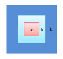
Figure 1: (Color online.) A schematic diagram showing the system $S$ immersed in environment $E$. The joint system $SE$ is in contact with a larger environment $E_{1}$.

Let us consider a particular subset of dynamical maps $\tilde{\Lambda}_{SE}^{\epsilon}$ such that that for any fixed $\epsilon\geq 0$, the time-evolved state $\tilde{\rho}^{SE}(t)$ satisfies the inequality

$$I_{Q}(\tilde{\rho}^{SE}(t))\leq\epsilon,\hskip 28.45274pt\forall\hskip 2.84544ptt,\rho^{S}_{0},\rho^{E}_{0},$$ (2)

where $I_{Q}(\varrho^{AB})=S(\varrho^{A})+S(\varrho^{B})-S(\varrho^{AB})$ is the quantum mutual information qmi-1 ; qmi-2 ; qmi-3 , of a bipartite state $\varrho^{AB}$, whereas $\varrho^{A}$ and $\varrho^{B}$ are respectively the reduced states of subsystems $A$ and $B$, and $S(\cdot)$ is the von Neumann entropy wehrl of its argument.

Let us mention here that in Ref. mairi-kono-connection-nei-kintu , the authors use the non-monotonicity in time-evolution of a classical and a quantum capacity of a map to define the non-Markovianity of that map. The classical capacity is defined in terms of quantum mutual information between the input and output of the channel. This is different from our approach, as we use the quantum mutual information in the system-environment output state of the evolution of the system-environment duo. The quantum capacity is defined by using a coherent information between the input and output of the map.

The quantum mutual information is a non-negative quantity, so that $I_{Q}(\tilde{\rho}^{SE}(t))$ in inequality (2) is lower bounded by zero. We will refer to the corresponding reduced maps $\tilde{\Lambda}_{S}^{\epsilon}$ of system $S$ as $\epsilon$-Markovian. The set of all such $\epsilon$-Markovian maps is denoted by $S^{\epsilon}$. Therefore, for the vanishing $\epsilon$ case, at every instant of time, the state of the system $S$ and the environment $E$ is a product state. However, the dynamical map $\Lambda_{SE}$ is not unitary in general. Hence, even in the case $\epsilon=0$, the dynamics of $S$ is not complete positive. This does not affect the classification of “$\epsilon$-Markovian” maps, since it does not depend on the definition of Markovianity in terms of divisibility. We will call the reduced dynamical maps on $S$ in the case $\epsilon=0$ as “Markovian-like” instead of “Markovian”. More about these maps has been discussed in Section V. See Kavan-ebang-Samya in this regard, where Markovian maps are defined by using the concept of a certain quantum process tensor.

It is to be noted that, a number of previous works have investigated non-Markovian dynamics by dividing the actual infinite dimensional environment into two parts pseudomode1 ; embedding ; reaction-coordinate ; NMV-core . One of them consists of finite number of degrees of freedom of the environment which significantly interacts with the system, the other is the residual infinite dimensional part. This separation leads to considerable mathematical simplicity while taking into account environmental interactions on the system dynamics, and often shows good agreement with experimental results. Depending on the crude details of identifying relevant environmental subsystems, the several approaches that has been proposed are Markovian-embedding embedding , pseudomode method pseudomode1 , reaction coordinate model reaction-coordinate , non-Markovian core model NMV-core etc. What remains common in these works, is that the non-Markovian dynamics of the system is attributed to the effective environment, whereas they together are treated with Born-markov approximation with respect to the residual environment. Unlike this, we do not consider a Markovian approximation between joint system $SE$ and $E_{1}$. Ours is a more general picture in which the correlation generated between $SE$ and $E_{1}$ depends on the dimension of $SE$, hence a Markovian approximation will be a very particular specialization.

III.3 Building an $\epsilon$-Markovian map

Let us consider the above definition in more detail. Markovian-like maps on $S$ are therefore those, which for any given product initial state between $S$, $E$, and $E_{1}$, does not create any correlation (as quantified by the quantum mutual information) between $S$ and $E$. This parallels the Born-Markov approximation in the “derivation” of the dynamics of open quantum systems, where at every time-step, that is much shorter than the typical time required for a nontrivial interaction between the system and its environment, the system is brought back to its initial state and all correlations between the system and the environment are removed. The $\epsilon$-Markovian maps are introduced in view of the fact that while almost no naturally occurring physical map is Markovian-like, there may be members of important families of maps that violate the criterion for being Markovian-like only “slightly”, in the sense of creating only a small amount of quantum mutual information for all time. Let us immediately provide an example of such a map, albeit an artificial one. Consider a qubit $S$ interacting with an “environment” $E$ which is also a qubit, and a bigger environment $E_{1}$ consisting of a large number of qubits. Initially, the state of the entire system is $|0\rangle_{S}|0\rangle_{E}|00\ldots\rangle_{E_{1}}$. A unitary $U_{SE}(1)$ acts on $SE$ to transform the state of $SE$ to $|\psi\rangle_{SE}=\alpha|00\rangle+\sqrt{1-|\alpha|^{2}}|11\rangle$, where $\alpha$ is a real number such that $I_{Q}(|\psi\rangle_{SE})=\epsilon$, for a previously chosen, possibly small, fixed real number $\epsilon\in[0,2]$. The joint system is four dimensional, hence defining the unitary on one particular basis will give rise to an infinite number of possibilities to define its action on the remaining three basis vectors. To unambiguously define the unitary, we will need to settle on its action on the remaining three basis vectors. We assume that this has been done. After this step, a swap operator acts on the qubit $E$ and a single qubit of $E_{1}$, so that the whole system is now

$$|\psi\rangle_{SE_{1}^{r}}|0\rangle_{E}|00\ldots\rangle_{E_{1}^{\bar{r}}},$$ (3)

where the superscript $r$ denotes a qubit of the environment $E_{1}$, while the superscript $\bar{r}$ denotes its complement. This entire evolution, viz. the action of the unitary $U_{SE}(1)$ and the swap operator, is to be considered as a single time-step. The state of $SE$ after this time step is $(|\alpha|^{2}|0\rangle\langle 0|+(1-|\alpha|^{2})|1\rangle\langle 1|)_{S}\otimes(|0\rangle\langle 0|)_{E}$. In the next time-step, we act with $U_{SE}(\epsilon_{1})=\exp{(i\epsilon_{1}H_{SE})}$, to create the state $\rho_{SE}$, where $U_{SE}(1)=\exp{(iH_{SE}})$, and where $\epsilon_{1}$ is chosen so that $I_{Q}(\rho_{SE})\leq\epsilon$. After this operation and still remaining within the same time-step, we swap the state of $E$ with the state of a qubit of $E_{1}$ that is still in $|0\rangle$. This second time-step is repeated again and again. We are assuming that $E_{1}$ has enough qubits to do these repetitions. We find that the construction of the dynamics is such that the quantum mutual information is never more than $\epsilon$, and thus, the above definition leads us to call it an $\epsilon$-Markovian map. In the entire construction of the map, we did not make any assumption that required us to go beyond quantum mechanics. We will discuss more about these issues later in the paper.

IV Measure of non-Markovianity and $\epsilon$-nonmarkovianity

It is to be noted that it is the amount of violation of $\epsilon$-Markovianity that we will refer as $\epsilon$-nonmarkovianity, and so it is really non-“$\epsilon$-Markovianity” that we will be dealing with. But we prefer to call it as $\epsilon$-nonmarkovianity to avoid a cumbersome nomenclature.

Our goal now is to quantify the non-Markovianity of a general dynamical map $\Lambda_{S}$ by its distance $\mathcal{D}$ from the $\epsilon$-Markovian maps $\tilde{\Lambda}_{S}^{\epsilon}$, minimized over the set $S^{\epsilon}$. We call it $\epsilon$-nonmarkovianity of the corresponding map $\Lambda_{S}$, and denote it by $N^{\epsilon}(\Lambda_{S})$. That is,

$$N^{\epsilon}\big{(}\Lambda_{S}(t)\big{)}=\min_{\tilde{\Lambda}_{S}^{\epsilon}\in S^{\large\epsilon}}\mathcal{D}\big{(}\Lambda_{S}(t)||\tilde{\Lambda}_{S}^{\epsilon}(t)\big{)}.$$ (4)

The distance $\mathcal{D}$ on the space of maps can be conceptualized in a variety of ways. Later on, we will use the Choi-Jamiołkowski-Kraus-Sudarshan (CJKS) isomorphism CJKS to define it. Now however, we define it by a maximization over the density operators on which the relevant maps act. More precisely, we define

$$\mathcal{D}(\Lambda||\Lambda^{\prime})=\max_{\rho}\mathbf{D}(\Lambda(\rho)||\Lambda^{\prime}(\rho))$$ (5)

where $\mathbf{D}$ is a distance measure defined on the space of density operators, which forms the domain of the maps involved in $\mathcal{D}$. See Refs. leditzky in this regard, which uses the concept of a generalized channel divergence between a channel and a set of channels, and which may also be used to quantify the distance we use in the space of channels.

We therefore have

$$N^{\epsilon}(\Lambda_{S})=\min_{\tilde{\Lambda}_{S}^{\epsilon}\in S^{\large\epsilon}}\max_{\rho^{S}_{0}}\mathbf{D}\big{(}\Lambda_{S}(\rho_{0}^{S})||\tilde{\Lambda}_{S}^{\epsilon}(\rho_{0}^{S})\big{)},$$ (6)

where we have involved ourselves in an additional maximization over all the initial states $\rho_{0}^{S}$. For a fixed $\tilde{\Lambda}_{S}^{\epsilon}$, if $\bar{\rho}^{S}_{0}$ is the state that maximizes $\mathbf{D}(\Lambda_{S}(\rho_{0}^{S})||\tilde{\Lambda}_{S}^{\epsilon}(\rho_{0}^{S}))$, then

$$\mathbf{D}\big{(}\Lambda_{S}(\bar{\rho}_{0}^{S})||\tilde{\Lambda}_{S}^{\epsilon}(\bar{\rho}_{0}^{S})\big{)}\leq\mathbf{D}\big{(}\Lambda_{SE}(\bar{\rho}^{S}_{0}\otimes\rho^{E}_{0})||\tilde{\Lambda}^{\epsilon}_{SE}(\bar{\rho}^{S}_{0}\otimes\rho^{E}_{0})\big{)}$$ (7)

where we have assumed that the distance $\mathbf{D}$ satisfies the inequality $\mathbf{D}($tr${}_{p}\sigma||$ tr${}_{p}\varrho)\leq\mathbf{D}(\sigma||\varrho)$, where tr_p is partial trace over the system denoted by “$p$”. Examples of such distances are trace-norm, relative entropy, etc. wehrl ; books-qic ; wilde1 ; channel_distance .

In the special case $\epsilon=0$, the minimization in Eq. (4) will be over maps that lead to time-evolved states $\tilde{\rho}^{SE}(t)$ for which $I_{Q}(\tilde{\rho}^{SE}(t))=0$, $\forall t,\rho^{S}_{0},\rho^{E}_{0}$. $I_{Q}(\rho^{AB})=0$ implies that the state $\rho^{AB}$ is a product of individual states of the component systems. A product state for $SE$ at all times for an initial product state of $SE$ can appear in the following way.

The evolution of $SEE_{1}$ is unitary, which can be global (i.e., entangling), and hence, the entanglement and other classical and quantum correlations HHHH ; bera that arise between $S$ and $EE_{1}$ may remain between parts of $S$ and parts of $EE_{1}$ or between the wholes ($S$ and $EE_{1}$), unless the unitary is very special. However, it may so happen that the interaction between $S$ and $E$ is weaker (or equivalently, the information flow between $S$ and $E$ is slower) than that between $E$ and $E_{1}$, so that any entanglement (or other correlations) created between $S$ and $E$ are transferred, and consequently hidden, in entanglement (or other correlations) between $S$ and $E_{1}$. In other words, after an interaction between $S$ and $E$, the state of $E$ at a given time $t$, is quickly transferred into the recesses of $E_{1}$, and replaced with a $\rho_{0}^{E}$, which has no correlations with $S$, and this is done before the next interaction of $E$ with $S$ starts off. We denote the set of all such reduced dynamical maps by $S^{0}$, and call them as Markovian-like, as discussed in Section II.

The description above is close to the collision model collision , though having the difference that the interaction of $S$ and $E$ is not unitary, as described in collision model. In this sense, the scenario we consider is a more general picture. Indeed, some assumptions are similar, e.g., $E$ never gets replaced with that part of $E_{1}$ which already shares correlation with $S$, and that $E_{1}$ is infinitely large. In the special case of $\Lambda_{SE}$ being unitary, our model becomes same as collision model.

V Behavior of distance based non-Markovianity measure

Next, we want to numerically investigate the behaviour of the distance based measure of non-Markovianity. As discussed in the beginning, calculating $\epsilon$-nonmarkovianity for a non-zero $\epsilon$ is numerically challenging. Nevertheless, in order to get an idea about how a distance based measure will behave temporally, we resort to the usual picture of Markovian and non-Markovian maps in terms of their divisibility. As we will see below, a distance measure can indeed capture the traits of a non-markovian dynamics.

V.1 Amplitude damping channel

To exemplify the behavior of non-Markovianity, we consider an amplitude damping channel books-qic ; Myatt ; Turchette ; Chirolli ; victor ; Zou ; pirandola-old ; wilde2 ; pirandola_new . The explicit example is taken from Ref. victor . The channel has the Lindblad generator $\mathcal{L}(\rho(t))$ given by

$$\mathcal{L}(\rho(t))=\sigma_{-}\rho(t)\sigma_{+}-\dfrac{1}{2}\{\sigma_{+}\sigma_{-},\rho(t)\},$$ (8)

where $\sigma_{-}$ and $\sigma_{+}$ are the qubit raising and lowering operators, and we are in the limit of a zero temperature bath. The corresponding master equation is $\dot{\rho}=\gamma_{a}(t)\mathcal{L}(\rho(t))$, where we choose the time-dependent “decay rate” $\gamma_{a}(t)$ as victor

$$\gamma_{a}(t)=\dfrac{2\lambda\gamma_{0}\sinh\ \dfrac{tg}{2}}{g\cosh\ \dfrac{tg}{2}+\lambda\sinh\ \dfrac{tg}{2}},~{}~{}g=\sqrt{\lambda^{2}-2\gamma_{0}\lambda}.$$ (9)

Here, $\gamma_{0}$ and $\lambda$ are two system parameters that can be used to decide about the Markovianity in terms of divisibility of the dynamics, as shown by Mukherjee et al. victor . When $\lambda>2\gamma_{0}$, the evolution is divisible and when $\gamma_{0}>\lambda/2$, the evolution is non-divisible. The non-divisible map $\Lambda_{S}$ is constructed by choosing a particular pair of values of $\gamma_{0}$ and $\lambda$ such that $\gamma_{0}>\lambda/2$. Keeping the value of $\lambda$ the same as that for the non-divisible map, we generate a class of divisible maps $\tilde{\Lambda}_{S}^{0}$, by randomly choosing $\gamma_{0}$, from a uniform distribution, while satisfying the condition $\lambda>2\gamma_{0}$. In parallel, we also generate the set of all density operators $\rho^{S}_{0}$ on $\mathbb{C}^{2}$ by Haar-uniformly generating pure states on the larger Hilbert space $\mathbb{C}^{2}\otimes\mathbb{C}^{2}$. The generation of the density matrices is therefore according to the “induced metric” karol ; induced . We now apply both the maps on the elements of this set of density operators to obtain the time evolved states $\Lambda_{S}(\rho^{S}_{0})$ and $\tilde{\Lambda}_{S}^{0}(\rho^{S}_{0})$, and maximize the trace distance between them over this set of density operators. The “trace distance” between two density matrices $\varrho$ and $\varsigma$ is given by $\mbox{tr}\sqrt{(\varrho-\varsigma)(\varrho-\varsigma)^{\dagger}}$. The trace distance thus obtained, is further minimized over the set of divisible maps generated by varying $\gamma_{0}$ for a fixed $\lambda$, with $\lambda>2\gamma_{0}$. The entire optimization process is executed for different points on the $t$-axis. The data is presented in Fig. 2 as the red solid curve. The non-Markovianity increases initially, starting to decrease after a certain time and then decaying to zero, i.e. the map becomes Markovian after a time. It is important to mention here that the optimization is performed under the assumption that the optimal Markovian-like map for a given non-divisible amplitude damping channel is attained within the class of divisible amplitude damping channels.

It is of course true that time-dependence in the parameters of the dynamical equation are not necessary for the optimization process, as only the outputs of the non-divisible channel and the nearest divisible channel are used in the definition of the non-Markovianity measure. But this is true if we are able to consider the optimization over all Markovian-like maps. This we have been unable to perform. We have therefore considered the time-dependent decay rates for all times for optimization process. For every time, it provides another element of the space of divisible maps, and gives us a chance of having a better estimate of the non-Markovianity measure.

While the optimization is carried out under the assumption that the optimal Markovian-like map will be obtained from within the class from which the non-divisible map is chosen, the “$\epsilon$-entanglement bound” on the $\epsilon$-nonmarkovianity measure, that we obtain below, is independent of these assumptions.

V.2 Phase damping channel

Besides the amplitude damping channel, we also want to investigate how $N^{\epsilon}(\Lambda_{S})$ behaves during evolution through a phase damping channel books-qic ; Luczka ; Palma ; HJM . The explicit form of the channel is taken from Ref. HJM . The master equation of the phase damping channel is

$$\dfrac{d\rho}{dt}=\frac{1}{2}\gamma(t)[\sigma_{z}\rho(t)\sigma_{z}-\rho],$$ (10)

where $\sigma_{z}$ is the Pauli $z$-matrix. We choose the time-dependent “dephasing rate”, $\gamma(t)$, as HJM

$$\gamma(t)=\int d\omega J(\omega)\coth(\hbar\omega/2k_{B}T)\sin(\omega t)/\omega,$$ (11)

where the integration is over the frequency of the bath-modes denoted by $\omega$, $J(\omega)$ is the “spectral function” of the bath. If we take our bath of consideration to have Ohmic-like spectra, then the spectral function is

$$J(\omega)=\frac{\omega^{s}}{\omega_{c}^{s-1}}e^{-\omega/\omega_{c}},$$ (12)

where $\omega_{c}$ is the “frequency cut-off”, and $s$ is the “Ohmicity parameter”, which decides whether the bath will be Ohmic ($s=1$), sub-Ohmic ($0<s<1$), or super-Ohmic ($s>1$). Keeping attention at the absolute zero temperature limit, we get the following expression for the dephasing rate:

$$\gamma_{\bar{0}}(t)=\omega_{c}[1+(\omega_{c}t)^{2}]^{-s/2}\Gamma(s)\sin[s\arctan(\omega_{c}t)],$$ (13)

where $\Gamma(s)$ denotes the Gamma function, given by $\Gamma(s)=\int_{0}^{\infty}x^{s-1}\exp{(-x)}dx$. While the Gamma function can be generalized to more general values of $s$, we will only use it for real $s>0$. In HJM , Haikka et al. have demonstrated that the non-divisibility of this channel is observed only when $s>2$. To numerically study $N^{\epsilon}(\Lambda_{S})$ for a non-divisible map, we take a particular value of $s=s_{NM}$, such that $s_{NM}>2$, corresponding to the map $\Lambda_{S}$. We generate $2000$ values of $s=s_{M}$ in the interval $0<s<2$, each corresponding to a divisible map, and for each $s_{M}$, we Haar-uniformly generate $2000$ random density matrices. The optimized $N^{\epsilon}(\Lambda_{S})$ has been presented in Fig. 3 with respect to the $\omega_{c}t$ along the horizontal axis. Similar to the amplitude damping channel, the non-Markovianity increases at first, reaches a maximum, then decays to zero. Notably, it revives again from zero after a time-interval. This non-monotonic behaviour of several physical quantities associated to the system is typical of a non-Markovian dynamics.

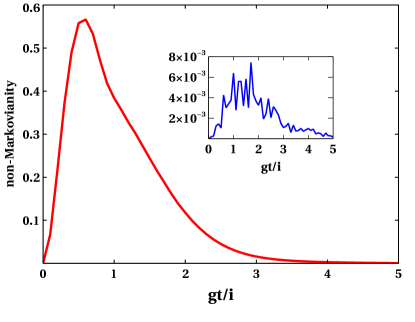
Figure 2: (Color online.) Non-Markovianity of the amplitude damping channel for the “max-distance” (red-solid curve) approach. We plot the non-Markovianity of the amplitude damping channel for $\lambda\kappa=4$, $\gamma_{0}\kappa=4$, where $\kappa$ is a constant having the unit of time. Note that for such choice of $\lambda\kappa$ and $\gamma_{0}\kappa$, $g\kappa$ is purely imaginary. The horizontal axis represents $gt/i$, while the vertical one represents non-Markovianity for $\epsilon=0$. Both axes are dimensionless. The distance between two density matrices is calculated by using the trace distance. The Haar-uniform searches are performed over $2000$ values of the pair $\gamma_{0}$, and over $2000$ density matrices, for each value of $gt/i$. In the inset, the blue solid curve is the non-Markovianity in “min-distance” approach (see Section VIII), for the same choice of parameters. Note that the increased oscillations in the min distance approach is possibly a numerical artefact, and if we disregard them, the general trend of the curves for min- and max-distance approaches are similar.

VI Entanglement-based bound on non-Markovianity

Going back to the scenario of general channels, but still remaining with the case when $\epsilon=0$, we have

$$\mathbf{D}\big{(}\Lambda_{SE}(\bar{\rho}^{S}_{0}\otimes\rho^{E}_{0})||\tilde{\Lambda}^{0}_{SE}(\bar{\rho}^{S}_{0}\otimes\rho^{E}_{0})\big{)}\geq E\big{(}\Lambda_{SE}(\bar{\rho}^{S}_{0}\otimes\rho^{E}_{0})\big{)},$$ (14)

where $E$ is a distance-based entanglement defined as the minimum distance of a state from the set of separable states HHHH . The inequality (14) holds by virtue of the fact that $\tilde{\Lambda}_{SE}^{0}(\bar{\rho}_{0}^{S}\otimes\rho_{0}^{E})$ is a separable and indeed a product state. In case the distance $\mathbf{D}$ is the relative entropy on the space of density operators, $E$ is the relative entropy of entanglement VPRK ; vedral of its argument. Let us now assume that $\mathbf{D}$ satisfies the triangle inequality, which is in fact not satisfied by relative entropy distance. We then obtain

$$\mathbf{D}\big{(}\Lambda_{SE}(\bar{\rho}^{S}_{0}\otimes\rho^{E}_{0})||\tilde{\Lambda}^{0}_{SE}(\bar{\rho}^{S}_{0}\otimes\rho^{E}_{0})\big{)}\leq E\big{(}\Lambda_{SE}(\bar{\rho}^{S}_{0}\otimes\rho^{E}_{0})\big{)}+d,$$ (15)

where $d$ is the “diameter” of the convex set of separable states ZHL . The diameter, $d$, of a set $\mathcal{S}$, is defined as

$$d(\mathcal{S})=\max_{\rho,\sigma\in\mathcal{S}}\mathbf{D}(\rho,\sigma)$$ (16)

A geometric representation of the relation (15) is given in Fig. 4. By combining relations (7) and (15) with definitions (4) and (6), we have

$$N^{0}(\Lambda_{S})\leq E\big{(}\Lambda_{SE}(\bar{\rho}^{S}_{0}\otimes\rho^{E}_{0})\big{)}+d.$$ (17)

This relation is true for all extensions of $\Lambda_{S}$ into $\Lambda_{SE}$ and for all $\rho_{0}^{E}$. Consequently,

$$N^{0}(\Lambda_{S})\leq\min_{\rho_{0}^{E},\Lambda_{SE}}[E\big{(}\Lambda_{SE}(\bar{\rho}^{S}_{0}\otimes\rho^{E}_{0})\big{)}+d],$$ (18)

where the minimization is over all $\rho_{0}^{E}$ and over all extensions of $\Lambda_{S}$ into $\Lambda_{SE}$. Note that the diameter $d$ is inside the optimization process, and not independent of it.

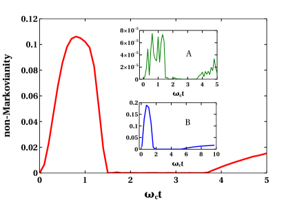
Figure 3: (Color online.) Non-Markovianity of the phase damping channel with respect to time $t$ for “max-distance” (red-solid curve) approach, where $s_{NM}=2.5$. The non-Markovianity decays, remains zero for finite interval, and then revives again. Inset:(A) Non-markovianity of the phase damping channel for “min-distance” approach (see Section VIII) when $s_{NM}=2.5$. (B) Non-Markovianity of the phase damping channel in “max-distance” approach when $s_{NM}=2.8$. Both the decay and revival occurs at later times compared to the case when $s_{NM}=2.5$.

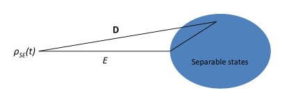
Figure 4: (Color online.) Geometric representation of the inequality between non-Markovianity and system-environment entanglement. We consider the case of $\epsilon=0$. The shaded region represents the convex set of states that are separable in the system-environment bipartition. The optimal state that attains the optimization in the definition of non-Markovianity is on or inside the set of separable states. The distance of this state to the time-evolved state $\rho_{SE}(t)$ must be greater than the sum of the other two sides of the triangle depicted in the figure. These latter sides however are respectively a distance-based entanglement of the evolved state and a bound on the diameter of the set of separable states. We have assumed that the distance measure on the space of density matrices satisfies the triangle inequality.

VII $\epsilon$-entanglement and $\epsilon$-nonmarkovianity

We now consider the general case, i.e., when $\mathbf{\epsilon\neq 0}$. In this case, the time evolved state $\tilde{\rho}^{SE}(t)=\tilde{\Lambda}^{\epsilon}_{SE}(\bar{\rho}^{S}_{0}\otimes\rho^{E}_{0})$ is no longer a product state, and instead it satisfies the inequality $I(\tilde{\Lambda}^{\epsilon}_{SE}(\bar{\rho}^{S}_{0}\otimes\rho^{E}_{0}))\leq\epsilon$, a weaker condition, that does not require the argument to be product (for $\epsilon\neq 0$). The set of all states $\eta^{SE}$ that satisfy $I_{Q}(\eta^{SE})\leq\epsilon$ does not form a convex set; however the set of convex combinations of all such states is of course a convex set and we call this set as the set of $\epsilon$-separable states. For $\epsilon=0$, this set becomes the set of convex combinations of product states, i.e. the set of separable states which have non-zero classical correlation. However, to calculate $\epsilon$-nonmarkovianity in the case $\epsilon=0$, we still need to minimize the distance function from the set of product states itself. In the present case of $\epsilon\neq 0$, the minimum distance possible between $\Lambda_{SE}(\bar{\rho}^{S}_{0}\otimes\rho^{E}_{0})$ and the set of $\epsilon$-separable states, is referred to as $\epsilon$-entanglement, $E^{\epsilon}$, of the state $\tilde{\rho}^{SE}(t)$. In case we use the relative entropy as a measure of distance, this is denoted by $E_{R}^{\epsilon}$.

We take a short break here from the main stream of the paper, and prove that the entanglement, as quantified by the relative entropy of entanglement VPRK ; vedral (denoted by $E_{R}$), of an arbitrary two-party quantum state whose $\epsilon$-entanglement is vanishing, cannot be higher than $\epsilon$. This, we believe, would go some way in legitimizing the use of the term “$\epsilon$-entanglement, as for small $\epsilon$, only weakly entangled states would have zero $\epsilon$-entanglement. Let us consider the two-party quantum state $\rho_{AB}$ such that $E_{R}^{\epsilon}(\rho_{AB})=0$. Therefore, by definition, $I_{Q}(\rho_{AB})\leq\epsilon$. Now, as we have already mentioned, the quantum mutual information of a bipartite state is the relative entropy distance of it from the tensor product of its local parts, and the latter is a separable state. Therefore, by definition of the relative entropy of entanglement, $E_{R}(\rho_{AB})\leq I_{Q}(\rho_{AB})$, so that $E_{R}(\rho_{AB})\leq\epsilon$.

Going back to where we left before the last paragraph, if $d_{\epsilon}$ is the diameter of the set of $\epsilon$-separable states, we get the following inequality:

$$\mathbf{D}\big{(}\Lambda_{SE}(\bar{\rho}^{S}_{0}\otimes\rho^{E}_{0})||\tilde{\Lambda}^{\epsilon}_{SE}(\bar{\rho}^{S}_{0}\otimes\rho^{E}_{0})\big{)}\leq E^{\epsilon}\big{(}\Lambda_{SE}(\bar{\rho}^{S}_{0}\otimes\rho^{E}_{0})\big{)}+d_{\epsilon}.$$ (19)

In this case, the relation (18) is replaced by

$$N^{\epsilon}(\Lambda_{S})\leq\min_{\rho_{0}^{E},\Lambda_{SE}}[E^{\epsilon}\big{(}\Lambda_{SE}(\bar{\rho}^{S}_{0}\otimes\rho^{E}_{0})\big{)}+d_{\epsilon}].$$ (20)

VIII The min-distance

The measures of non-Markovianity and $\epsilon$-nonmarkovianity depended, among other things, on the fact that we perform a maximization over the set of density matrices on the system $S$. See Eq. (5). Let us refer to this strategy as that of “max-distance”. This however is hardly a unique strategy, and in particular, one can certainly define the distance between the maps by using a minimization over the density operators, i.e., by using the distance

$$\mathcal{D}_{m}(\Lambda||\Lambda^{\prime})=\min_{\rho}\mathbf{D}(\Lambda(\rho)||\Lambda^{\prime}(\rho)).$$ (21)

So, the definition of non-Markovianity accordingly changes to

$$N^{\epsilon}_{m}(\Lambda_{S})=\min_{\tilde{\Lambda}_{S}^{\epsilon}\in S^{\large\epsilon}}\min_{\rho^{S}_{0}}\mathbf{D}\big{(}\Lambda_{S}(\rho_{0}^{S})||\tilde{\Lambda}_{S}^{\epsilon}(\rho_{0}^{S})\big{)}.$$ (22)

We refer to this approach as that of the “min-distance”. Suppose that for a fixed $\tilde{\Lambda}_{S}^{\epsilon}$, $\bar{\bar{\rho}}_{0}^{S}$ is the state that minimizes $\mathbf{D}(\Lambda_{S}(\rho_{0}^{S})||\tilde{\Lambda}_{S}^{\epsilon}(\rho_{0}^{S}))$. Proceeding as in the case of “max-distance”, we can see that in the special case of $\mathbf{\epsilon=0}$, the relation (15) changes to

$$\mathbf{D}\big{(}\Lambda_{SE}(\bar{\bar{\rho}}^{S}_{0}\otimes\rho^{E}_{0})||\tilde{\Lambda}^{0}_{SE}(\bar{\bar{\rho}}^{S}_{0}\otimes\rho^{E}_{0})\big{)}\leq E\big{(}\Lambda_{SE}(\bar{\bar{\rho}}^{S}_{0}\otimes\rho^{E}_{0})\big{)}+d.$$ (23)

Accordingly, the relation (18) changes to

$$N^{0}_{m}(\Lambda_{S})\leq\min_{\rho_{0}^{E},\Lambda_{SE}}[E\big{(}\Lambda_{SE}(\bar{\bar{\rho}}^{S}_{0}\otimes\rho^{E}_{0})\big{)}+d],$$ (24)

where the entanglement function is the same as before, while the actual quantity has changed to $E\big{(}\Lambda_{SE}(\bar{\bar{\rho}}^{S}_{0}\otimes\rho^{E}_{0})\big{)}$, in contrast to $E\big{(}\Lambda_{SE}(\bar{\rho}^{S}_{0}\otimes\rho^{E}_{0})\big{)}$ in the “max-distance” case.

The $\epsilon\neq 0$ can be similarly derived. It is important to stress here that despite the similarity of notation and the algebra, we have here a completely independent bound on an independent measure of non-Markovianity of a general dynamical map $\Lambda_{S}$, as compared to the case of “max-distance”.

Similar to the case of “max-distance”, here also, we have numerically studied the behavior of non-Markovianity for the amplitude damping channel. This is presented in the inset of Fig. 2. The corresponding diagram for the phase damping channel is an inset of Fig. 3. The value of the optimized distance is very small ($\sim 10^{-3}$-$10^{-5}$). The size of the set used for optimization is not large enough in this case for the first significant digit to converge, despite the simulation taking long time. This leads to the oscillatory behaviour observed in the figures corresponding to “min-distance”. Nevertheless the envelope of the oscillations has an overall same behavior as that observed in the max-distance approach.

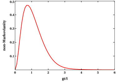
Figure 5: (Color online.) Non-Markovianity of the amplitude damping channel in the CJKS approach for $\lambda\kappa=4$, $\gamma_{0}\kappa=10$, The notations in this figure remain the same as in Fig. 2, except that the non-Markovianity is defined here from the CJKS approach, and that the curve is plotted by simply joining the data points.

IX The CJKS approach to non-Markovianity

In the analysis until now, we have defined distance on the space of maps by using a distance on the space of density operators on which the maps act and a corresponding double optimization. See Eqs. (5) and (21). However, instead of using these approaches (viz., the “max-distance” and the “min-distance” ones), in Eq. (4), we may define the distance on the space of maps on $S$ by using the CJKS representation in the following way. We define

$$\mathcal{D}(\Lambda||\Lambda^{\prime})=\mathbf{D}(\mathbf{I}\otimes\Lambda(|\Psi^{+}\rangle\langle\Psi^{+}|)||\mathbf{I}\otimes\Lambda^{\prime}(|\Psi^{+}\rangle\langle\Psi^{+}|))$$ (25)

where $|\Psi^{+}\rangle=\dfrac{1}{\overline{d}^{\frac{1}{2}}}\sum_{i=0}^{\overline{d}-1}|ii\rangle$, and $\mathbf{I}$ is the identity map on the space of operators on a “reference” Hilbert space, $H_{R}$, which has the same dimension $\overline{d}$, as $H_{S}$. Note that $|\Psi^{+}\rangle$ is an element of $H_{R}\otimes H_{S}$. This approach inherits the properties of the CJKS representation, and in particular has the benefit of a reduced level of optimization, as compared to the preceding approach. In Fig. 5, we provide a numerical calculation to exemplify the behavior of the non-Markovianity when seen through this approach, for the amplitude damping channel.

X Conclusion

To conclude, we have considered a measure of non-Markovianity of a dynamical map on an open quantum system based on the distance of the dynamical map on the reduced system from the set of all “Markovian-like” dynamical maps on the same system. We found a quantitative relation between the measure, and the entanglement between the reduced system and the environment. This relation can be used to estimate one of the quantities if we are able to find the other. To exemplify the notion and the relation, we have studied amplitude damping and phase damping channels.

Along with considering the case when the maps are exactly Markovian-like, we have also considered the situation when a map violates the Markovian-like property but only a “little”. This is quantified by introducing the concept of $\epsilon$-Markovianity. Correspondingly, we present the notion of being outside this set, and quantify it by proposing the concept of $\epsilon$-nonmarkovianity. We then went on to generalize the entanglement-based bound on non-Markovianity mentioned above to the $\epsilon\neq 0$ case, by suggesting a notion of $\epsilon$-separability and $\epsilon$-entanglement.

- (1) H.-P. Breuer and F. Petruccione, The theory of open quantum systems (Oxford University Press, Oxford, 2002).
- (2) H.-P. Breuer, J. Phys. B: At. Mol. Opt. Phys. 45, 154001 (2012); Á. Rivas and S. F. Huelga, Open Quantum Systems: An Introduction (Springer, Heidelberg, 2012); H.-P. Breuer, E.-M. Laine, J. Piilo, and B. Vacchini, Rev. Mod. Phys. 88, 021002 (2016); I. de Vega and D. Alonso, Rev. Mod. Phys. 89, 015001 (2017).
- (3) L. Li, M. J. W. Hall, and H. M. Wiseman, Phys. Rep. 759, 1 (2018).
- (4) Á. Rivas, S. F. Huelga, and M. B. Plenio, Rep. Prog. Phys. 77, 094001 (2014).
- (5) Á. Rivas, S. F. Huelga, and M. B. Plenio, Phys. Rev. Lett. 105, 050403 (2010).
- (6) M. M. Wolf, J. Eisert, T. S. Cubitt, and J. I. Cirac, Phys. Rev. Lett. 101, 150402 (2008); M. M. Wolf and J. I. Cirac, Commun. Math. Phys. 279, 147 (2008).
- (7) S. C. Hou, X. X. Yi, S. X. Yu, and C. H. Oh., Phys. Rev. A 83, 062115 (2011).
- (8) X.-M. Lu, X. Wang, and C. P. Sun, Phys. Rev. A 82, 042103 (2010).
- (9) A. K. Rajagopal, A. R. Usha Devi, and R. W. Rendell, Phys. Rev. A 82, 042107 (2010).
- (10) S. Luo, S. Fu, and H. Song, Phys. Rev A 86, 044101, (2012).
- (11) S. Lorenzo, F. Plastina, and M. Paternostro, Phys. Rev. A 88, 020102(R), (2013).
- (12) F. F. Fanchini, G. Karpat, B. Çakmak, L. K. Castelano, G. H. Aguilar, O. Jiménez Farías, S. P. Walborn, P. H. Souto Ribeiro, and M. C. de Oliveira, Phys. Rev. Lett. 112, 210402 (2014).
- (13) S. Salimi, S. Haseli, A.S. Khorashad, and F. Adabi, Int. J. Theo. Phys. 55, 4089 (2016).
- (14) H. S. Dhar, M. N. Bera, and G. Adesso, Phys. Rev. A 91, 032115 (2015).
- (15) T. Chanda and S. Bhattacharya, Annals of Physics 366, 1 (2016).
- (16) H.-P. Breuer, E.-M. Laine, and J. Piilo, Phys. Rev. Lett. 103, 210401 (2009).
- (17) S. Wißmann, A. Karlsson, E.-M. Laine, J. Piilo, and H.-P. Breuer, Phys. Rev. A 86, 062108 (2012).
- (18) E.-M Laine, J. Pillo, and H.-P Breuer, Phys. Rev. A 81, 062115, (2010).
- (19) L. Mazzola, E.-M. Laine, H.-P. Breuer, S. Maniscalco, and J. Piilo, Phys. Rev. A 81, 062120 (2011).
- (20) T. J. G. Apollaro, C. D. Franco, F. Plastina, and M. Paternostro, Phys. Rev. A 83, 032103 (2011).
- (21) P. Haikka, J. D. Cresser, and S. Maniscalco, Phys. Rev. A 83, 012112 (2011).
- (22) D. Chruscinski, A. Kossakowski, and A Rivas, Phys. Rev. A 83, 052128 (2011).
- (23) M. Jiang and S. Luo, Phys. Rev. A 88, 034101 (2013).
- (24) P. F. Romero, K. Modi, and F. A. Pollock, Quantum 3, 136 (2019).
- (25) M. J. W. Hall, J. D. Cresser, L. Li, and E. Andersson, Phys. Rev. A 89 042120 (2014); J. Teittinen, H. Lyyra, B. Sokolov, and S. Maniscalco, New J. Phys. 20, 073012 (2018).
- (26) R. Horodecki, P. Horodecki, M. Horodecki, and K. Horodecki, Rev. Mod. Phys. 81, 865 (2009).
- (27) T. M. Cover and J. A. Thomas, Elements of Information Theory (Wiley, New Jersey, 1991).
- (28) R. L. Stratonovich, Radiofizika 8, 116 (1965) [English translation in Probl. Inform. Transm. 2, 35 (1966)]; W. H. Zurek, in Quantum Optics, Experimental Gravitation and Measurement Theory, edited by P. Meystre and M. O. Scully (Plenum, New York, 1983); S. M. Barnett and S. J. D. Phoenix, Phys. Rev. A 40, 2404 (1989); B. Schumacher and M. A. Nielsen, ibid. 54, 2629 (1996); N. J. Cerf and C. Adami, Phys. Rev. Lett. 79, 5194 (1997).
- (29) B. Groisman, S. Popescu, and A. Winter, Phys. Rev. A 72, 032317 (2005).
- (30) A. Wehrl, Rev. Mod. Phys. 50, 221 (1978).
- (31) H. Ollivier and W. H. Zurek, Phys. Rev. Lett. 88, 017901 (2001); L. Henderson and V. Vedral, J. Phys. A: Math. Gen. 34, 6899 (2001); J. Oppenheim, M. Horodecki, P. Horodecki, and R. Horodecki, Phys. Rev. Lett. 89, 180402 (2002); M. Horodecki, K. Horodecki, P. Horodecki, R. Horodecki, J. Oppenheim, A. Sen(De), and U. Sen, Phys. Rev. Lett. 90, 100402 (2003); M. Horodecki, P. Horodecki, R. Horodecki, J. Oppenheim, A. Sen(De), U. Sen, and B. Synak-Radtke, Phys. Rev. A 71 062307 (2005).
- (32) K. Modi, A. Brodutch, H. Cable, T. Paterek, and V. Vedral, Rev. Mod. Phys. 84, 1655 (2012); A. Bera, T. Das, D. Sadhukhan, S. S. Roy, A. Sen(De), and U. Sen, Rep. Prog. Phys. 81, 024001 (2018).
- (33) K. L. Chung, A Course in Probability Theory (Academic, New York, 1968); B. V. Gnedenko, Theory of Probability (Nauka, Moscow, 1988); C. W. Gardiner, Handbook of Stochastic Methods (Springer, Berlin, 1997).
- (34) P. Pechukas, Phys. Rev. Lett. 73, 1060 (1994).
- (35) B. Bylicka, D. Chruśiński, and S. Maniscalco. Scientific Reports 4, 5720 (2014).
- (36) F. A. Pollock, C. Rodríguez-Rosario, T. Frauenheim, M. Paternostro, and K. Modi, Phys. Rev. Lett. 120, 040405 (2018).
- (37) A. Imamog̃lu, Phys. Rev. A 50, 3650 (1994); P. Stenius and A. Imamog̃lu, Quantum Semiclass. Opt. 8, 283 (1996); G. Pleasance and B. M. Garraway, Phys. Rev. A 96, 062105 (2017); B. M. Garraway, Phys. Rev. A. 55, 2290 (1997); G. Pleasance, B. M. Garraway and F. Petruccione, Phys. Rev. Research 2, 043058 (2020).
- (38) R. S. Bennink and P. Lougovski, New J. Phys. 21, 083013 (2019); I. A. Luchnikov, S. V. Vintskevich, H. Ouerdane, and S. N. Filippov, Phys. Rev. Lett. 122, 160401 (2019); I. A. Luchnikov, S. V. Vintskevich, D. A. Grigoriev, and S. N. Filippov, Phys. Rev. Lett. 124, 140502 (2020); M. P. Woods, R. Groux, A. W. Chin, S. F. Huelga, and M. B. Plenio, J. Math. Phys. 55, 032101 (2014).
- (39) J. I. -Smith, A. G. Dijkstra, N. Lambert, and A. Nazir, J. Chem. Phys. 144, 044110 (2016); J. I. -Smith, N. Lambert, and A. Nazir, Phys. Rev. A. 90, 032114 (2014); P. Strasberg, G. Schaller, N. Lambert and T. Brandes, New J. Phys. 18, 073007 (2016).
- (40) D. Tamascelli, A. Smirne, S. F. Huelga and M. B. Plenio, Phys. Rev. Lett 120, 030402 (2018).
- (41) A. Jamiołkowski, Rep. Math. Phys. 3, 275 (1972); M.-D. Choi, Linear Alg. Appl. 10, 285 (1975); K. Kraus, States, effects, and operations: fundamental notions of quantum theory (Springer, Berlin, 1983); E. C. G. Sudarshan, Quantum Measurement and Dynamical Maps in ‘From SU(3) to Gravity’ (Cambridge University Press, Cambridge, 1986).
- (42) F. Leditzky, E. Kaur, N. Datta, and M. M. Wilde, Phys. Rev. A 97, 012332 (2018); Z. W. Liu and A. Winter, arXiv: 1904.04201 (2019).
- (43) M. A. Nielsen and I. L. Chuang, Quantum Computation and Quantum Information (Cambridge University Press, Cambridge, 2000).
- (44) M. M. Wilde, Quantum Information Theory (Cambridge University Press, Cambridge, 2013).
- (45) J. Watrous, The Theory of Quantum Information (Cambridge University Press, Cambridge, (2018).
- (46) J. Rau, Phys. Rev. 129, 1880 (1963); V. Scarani, M. Ziman, P. Štelmachovič, N. Gisin, and V. Bužek, Phys. Rev. Lett. 88, 097905 (2002); M. Ziman, P. Štelmachovič, V. Bužek, M. Hillery, V. Scarani, and N. Gisin, Phys. Rev A 65, 042105 (2002); M. Ziman and V. Bužek, Phys. Rev A 72, 022110 (2005); M. Ziman, P. Štelmachovič, and V. Bužek, Open Sys. Inf. Dyn. 12, 81 (2005); V. Giovannetti, J. Phys. A 38, 10989 (2005); S. Attal and Y. Pautrat, Ann. Inst. Henri Poincare 7, 59 (2006); C. Pellegrini and F. Petruccione, Journal of Physics A: Mathematical and Theoretical 42, 425304 (2009); V. Giovannetti and G. M. Palma, Phys. Rev. Lett. 108, 040401 (2012); V. Giovannetti and G. M. Palma, J. Phys. B 45, 154003 (2012); T. Rybár, S. N. Filippov, M. Ziman, and V. Bužek, J. Phys. B 45, 154006 (2012); F. Ciccarello, G. M. Palma, and V. Giovannetti, Phys. Rev A 87, 040103 (2013); F. Caruso, V. Giovannetti, C. Lupo, and S. Mancini, Rev. Mod. Phys. 86, 1203 (2014); S. Lorenzo, A. Farace, F. Ciccarello, G. M. Palma, and V. Giovannetti, Phys. Rev A 91, 022121 (2015); S. N. Filippov, J. Pillo, S. Maniscalco and M. Ziman, Phys. Rev. A 96, 032111 (2017); M. Cattaneo, G. D. Chiara, S. Maniscalco, R. Zambrini, G. L. Giorgi, Phys. Rev. Lett. 126, 130403 (2021); S. Campbell and B. Vaccini, EPL 133 60001 (2021).
- (47) C. J. Myatt, B. E. King, Q. A. Turchette, C. A. Sackett, D. Kielpinski, W. M. Itano, C. Monroe, and D. J. Wineland, Nature 403, 269 (2000).
- (48) Q. A. Turchette, C. J. Myatt, B. E. King, C. A. Sackett, D. Kielpinski, W. M. Itano, C. Monroe, and D. J. Wineland, Phys. Rev. A 62, 053807 (2000).
- (49) L. Chirolli and G. Burkard, Advances in Physics 57, 225, arXiv:0809.4716 (2008).
- (50) V. Mukherjee, V. Giovannetti, R. Fazio, S. F. Huelga, T. Calarco, and S. Montangero, New J. Phys. 17, 063031 (2015).
- (51) W.-J. Zou, Y.-H. Li, S.-C. Wang, Y. Cao, J. Ren, J. Yin, C.-Z. Peng, X.-B. Wang, and J.-W. Pan, Phys. Rev. A 95, 042342 (2017).
- (52) S. Pirandola, R. Laurenza, C. Ottaviani, and L. Banchi, Nat. Commun. 8, 15043 (2017).
- (53) S. Khatri, K. Sharma, and M. M. Wilde, arXiv:1903.07747 (2019).
- (54) L. Banchi, J. Pereira, S. Lloyd, and S. Pirandola, arXiv:1905.01318 (2019); L. Banchi, J. Pereira, S. Lloyd, and S. Pirandola, arXiv:1905.01316 (2019).
- (55) I. Bengtsson and K. Życzkowski, Geometry of quantum states: An Introduction to Quantum Entanglement (Cambridge University Press, Cambridge, 2006).
- (56) K. Życzkowski and H.-J. Sommers, J. Phys. A 34, 7111 (2001).
- (57) J. Luczka, Physica A 167, 919 (1990).
- (58) G. M. Palma, K.-A. Suominen, and A. K. Ekert, Proc. R. Soc. London, Ser. A 452, 567 (1996).
- (59) P. Haikka, T. H. Johnson, and S. Maniscalco, Phys. Rev. A 87, 010103 (R) (2013).
- (60) V. Vedral, M. B. Plenio, M. A. Rippin, and P. L. Knight, Phys. Rev. Lett. 78, 2275 (1997).
- (61) V. Vedral, Rev. Mod. Phys. 74, 197 (2002).
- (62) K. Życzkowski, P. Horodecki, A. Sanpera, and M. Lewenstein, Phys. Rev. A 58, 883 (1998); S. L. Braunstein, C. M. Caves, R. Jozsa, N. Linden, S. Popescu, and R. Schack Phys. Rev. Lett. 83, 1054 (1999); S. Szarek, Phys. Rev. A 72, 032304 (2005), and references therein.