Multi-Cap Optimization for Wireless Data Plans with Time Flexibility

Abstract

An effective way for a Mobile network operator (MNO) to improve its revenue is price discrimination, i.e., providing different combinations of data caps and subscription fees. Rollover data plan (allowing the unused data in the current month to be used in the next month) is an innovative data mechanism with time flexibility. In this paper, we study the MNO’s optimal multi-cap data plans with time flexibility in a realistic asymmetric information scenario. Specifically, users are associated with multi-dimensional private information, and the MNO designs a contract (with different data caps and subscription fees) to induce users to truthfully reveal their private information. This problem is quite challenging due to the multi-dimensional private information. We address the challenge in two aspects. First, we find that a feasible contract (satisfying incentive compatibility and individual rationality) should allocate the data caps according to users’ willingness-to-pay (captured by the slopes of users’ indifference curves). Second, for the non-convex data cap allocation problem, we propose a Dynamic Quota Allocation Algorithm, which has a low complexity and guarantees the global optimality. Numerical results show that the time-flexible data mechanisms increase both the MNO’s profit (25% on average) and users’ payoffs (8.2% on average) under price discrimination.

1 Introduction

1.1 Background and Motivation

Mobile Network Operators (MNOs) profit from the wireless data services through carefully designing their wireless data plans. The pricing strategy involved in the wireless data plans has evolved from the flat-rate scheme to the usage-based scheme in the past years [3]. Now the most widely used data plan consists of a monthly data cap, a monthly one-time subscription fee, and a linear price for any unit of additional data consumption beyond the data cap. Based on this pricing strategy, MNOs usually offer multiple data caps together with different monthly subscription fees for users to choose from. For example, in the US market, AT&T charges $20 for 300MB, $45 for 1GB, $55 for 2GB, and $70 for 4GB; and the linear price for exceeding the data cap is $15/GB [4].

The purpose of MNO’s multi-cap offering is to capture more user surplus by differentiating users based on their preferences, also called price discrimination in economics [5]. To make such a price discrimination scheme work, the MNO must be able to identify the market segments by users’ preferences that are usually users’ private information, and the MNO needs to enforce the scheme through some incentive mechanism. For example, the MNO may want to offer a larger monthly data cap with a larger monthly subscription fee to businessmen, who have a stronger ability to pay and a relatively inelastic data demand comparing with other consumers (such as students). However, it is a very challenging problem to induce users to truthfully reveal their private preferences in practice, especially when users have multi-dimensional private preferences. This motivates us to ask the first key question in this paper.

Question 1.

How should the MNO optimize the multi-cap data plan offering?

Recently the growing market competition forces the MNOs to explore various innovations on their mobile data plans. For example, the rollover data plan enables users to enjoy the time flexibility over their data consumptions, by allowing the unused data from the previous month to be used in the current month. Such a rollover mechanism is attractive to users, as a user’s data demand is often stochastic and the rollover mechanism helps users balance the possible data waste within the data cap and the possible overage usage when consuming beyond the data cap.

Although based on the same rollover principle, different rollover data plans are different in terms of the consumption priority between the rollover data and the monthly data cap. For example, the rollover data plan offered by AT&T requires that the rollover data from the previous month should be consumed after the current monthly data cap [6], while China Mobile requires the other way around [7]. In our previous work [8, 9], we analyzed the MNO’s optimal data plan with time flexibility under the single-cap scheme (without price discrimination) and found that the time flexibility can increase both the MNO’s profit and users’ payoff, hence improve the social welfare. This motivates us to ask the second key question in this paper.

Question 2.

What is the impact of time flexibility under the multi-cap scheme?

In this paper, we will study the MNO’s price discrimination through the multi-cap data plans, taking into account the time-flexible data mechanisms.

1.2 Solutions and Contributions

We study how the MNO optimizes its multi-cap data plans under different data mechanisms with time flexibility. Specifically, we consider an asymmetric information scenario, where the users’ preferences for the wireless data plans are private and multi-dimensional. We formulate this problem as a multi-dimensional contract design. More specifically, the MNO needs to design a contract (with different combinations of data caps and the corresponding subscription fees) for users of different types, so that each user will truthfully reveal his type (i.e., private preferences) by selecting a contract item intended for his type.

The key results and contributions of this paper are summarized as follows:

• Systematic Study on MNO’s Price Discrimination: To the best of our knowledge, this is the first work studying the MNO’s price discrimination through optimizing the multi-cap wireless data plans. We take into account both the time flexibility (of the rollover data mechanisms) and the realistic asymmetric information.

• Exploring Time Flexibility in Price Discrimination: We investigate three different data mechanisms (i.e., one traditional data mechanism and two rollover data mechanisms) and analyze the MNO’s multi-cap data plan optimization under the three data mechanisms in a common design framework.

• Solving the Optimal Contract: The MNO’s contract problem involves user’s multi-dimensional private information, hence is challenging to solve. We exploit the separable structure (between users’ types and quota allocation) of our problem and develop a tractable approach to solve the MNO’s contract problem. First, we find that the slope of a user’s indifference curve on the contract plane corresponds to his willingness-to-pay, and a feasible contract (satisfying the incentive compatibility and individual rationality conditions) should allocate the data caps according to users’ willingness-to-pay. This enables us to obtain the optimal prices for a particular data cap allocation in closed-form. Second, for the non-convex data cap allocation problem, we propose a Dynamic Quota Allocation Algorithm, which guarantees the global optimality with a low computational complexity.

• Performance Evaluation based on Empirical Data: We evaluate the optimal contract under different data mechanisms based on the empirical data. The numerical results show that the time-flexible data mechanisms increase both the MNO’s profit (25% on average) and users’ payoffs (8.2% on average) under the multi-cap price discrimination, hence improves the social welfare.

The remainder of this paper is organized as follows. In Section 2, we review the related works. Section 3 introduces the system model. Section 4 analyzes the contract feasibility and Section 5 studies the contract optimality. In Section 6, we present the numerical results. Finally, we conclude this paper in Section 7.

2 Literature Review

There have been many excellent studies on the wireless data plan optimizations (e.g., [10, 11, 12, 13]). However, they did not take into account the recently introduced rollover mechanism or the ubiquitous multi-cap scheme.

The rollover mechanisms have been studied in [14, 15, 8, 9, 16]. Zheng et al. in [14] found that moderately price-sensitive users can benefit from subscribing to the rollover data plan compared with the traditional data plan. Wei et al. in [15] studied the rollover period length from a profit-maximizing MNO’s perspective. In our previous works, we studied the optimization of the time-flexible data plans in [8] and investigated the impact of the market competition in [9] and the trading market in [16]. However, all of these studies were based on the single-cap scheme without considering the ubiquitous multi-cap adoption.

The MNO’s multi-cap offering was seldom studied in previous literature. Dai et al. in [17] considered a case where the MNO offers two different data caps, i.e., a cap of basic rate and a cap of premium rate. However, the analysis was difficult to be generalized to more than two data caps. Therefore, there is no existing systematic study on the MNO’s optimal multi-cap design, let alone under the time-flexible data mechanisms. A key challenge for this problem is that different users make their data cap choices based on their individual preferences, which are often private information and can be multi-dimensional. Hence the MNO needs to properly design multiple data caps to differentiate users without knowing their exact private information and maximize the MNO’s profit. Such a problem naturally leads to a contract design problem [18].

TABLE I: Comparing Related Literature.

Literature	Rollover Considered?	Multi-Cap Considered?
[10]-[13]	No	No
[8][9][14]-[16]	Yes	No
[17]	No	Yes (but limited)
This Paper	Yes	Yes

Users’ multi-dimensional private information leads to a multi-dimensional contract design problem. Such a problem is often very challenging, since the multi-dimensional private information makes it difficult to achieve the global incentive compatibility [19]. To address this problem, McAfee and McMillan in [20] proposed the generalized single-crossing condition to ensure the globally incentive compatibility for a contract problem with multi-dimensional private information, but such a strong condition is not satisfied in many models (including ours). Rochet and Chone in [21] developed a sweeping procedure which adjusts the solution to ensure the global incentive compatibility. Such an approach requires that the dimension of the type space and allocation space coincide (which is not applicable to the MNO’s multi-cap data plans optimization), and cannot be solved analytically except in very special cases. In this paper, we introduce users’ willingness-to-pay by investigating their indifference curves, based on which we can develop a tractable approach for the MNO to provide the global incentive to all user types and solve its optimal contract under multi-dimensional private information.

3 System Model

We formulate the MNO’s multi-cap data plan design as a three-step process as shown in Fig. 1. In Step I, the MNO collects data from the user market to estimate the statistical information of users’ individual preferences (i.e., a user’s type), which are often private and multi-dimensional information (hence difficult to predict on a per user basis). In Step II, the MNO chooses a data mechanism to provide the subscribers with time flexibility. Then in Step III, the MNO proceeds with the multi-cap contract design to induce users truthfully revealing their types and hence maximize the MNO’s profit. Generally speaking, the MNO should periodically (e.g., every year) repeat the three steps to capture users’ varying requirements (due to, for example, technology changes).

Furthermore, the MNO should extract as many dimensions of the user type as possible to characterize users’ private information precisely, which leads to a contract problem with multi-dimensional private information. As mentioned as Section I, a multi-dimensional contract is challenging to solve. In this paper, we exploit the separable structure (between the user’s types and the data cap allocation), and propose to characterize each type of users’ willingness-to-pay by investigating their indifference curves. To provide a clear demonstration, we use a two-dimensional user type to illustrate our approach.

Next we describe three data mechanisms in Section 3.1. Then we introduce users’ two-dimensional characteristics and derive users’ payoffs under different data mechanism in Section 3.2. Finally, we formulate the MNO’s optimal contract problem in Section 3.3.

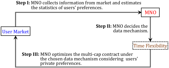
Figure 1: System model for the MNO’s multi-cap design.

3.1 Data Mechanisms

A mobile data plan can be characterized by the tuple $\mathcal{T}=\{Q,\Pi,\pi,\kappa\}$, where a subscriber pays a lump-sum subscription fee $\Pi$ for a data usage up to the monthly data cap $Q$, beyond which the MNO will charge an additional fee $\pi$ for each unit of data consumption. Here $\kappa\in\{0,1,2\}$ represents different data mechanisms that offer subscribers different time flexibilities on their data consumption over time.

The key differences among the three data mechanisms are the rollover data and consumption priority, both of which will affect the subscriber’s expected overage data consumption [8]. First, the rollover data from the previous month can enlarge a user’s effective data cap of the current month, within which no additional fee involved. Second, the consumption priorities of the rollover data and the monthly data cap further affect how much the effective cap is enlarged. In Table II, we use $\tau$ to denote a user’s rollover data from the previous month. More specifically,

• The case of $\kappa=0$ denotes the traditional data plan. The subscriber has no rollover data, and the effective cap of each month is $Q_{0}^{e}(\tau)=Q$;

• The case of $\kappa=1$ denotes the rollover data plan offered by AT&T. The rollover data $\tau\in[0,Q]$ from the previous month is consumed after the current monthly data cap $Q$. Thus the effective cap of the current month is $Q_{1}^{e}(\tau)=Q+\tau$;

• The case of $\kappa=2$ denotes the rollover data plan offered by China Mobile. The rollover data $\tau\in[0,Q]$ from the previous month is consumed prior to the current monthly data cap $Q$. Thus the effective cap of the current month is $Q_{2}^{e}(\tau)=Q+\tau$;

TABLE II: $\mathcal{T}\triangleq\{Q,\Pi,\pi,\kappa\},\ \kappa\in\{0,1,2\}$.

Plan	Rollover Data $\tau$	Consumption Priority	$Q_{\kappa}^{e}(\tau)$
$\kappa=0$	0	Cap	$Q$
$\kappa=1$	$\tau\in[0,Q]$	Cap$\Rightarrow$Rollover	$Q+\tau$
$\kappa=2$	$\tau\in[0,Q]$	Rollover$\Rightarrow$Cap	$Q+\tau$

As we mentioned above, the time flexibility can enlarge the subscriber’s effective data cap. According to Table II, the effective data cap of the traditional data mechanism $\kappa=0$ is always $Q$. However, for $\kappa\in\{1,2\}$, the effective data cap is $Q+\tau$, which is no smaller than $Q$ in the traditional data mechanism. Although $\kappa=1$ and $\kappa=2$ lead to the same expression $Q+\tau$, the stationary distribution of $\tau$ is different for $\kappa\in\{1,2\}$. Intuitively, the larger the effective data cap is, the less additional payment is incurred, which will further change users’ subscription choices.

3.2 User Model

3.2.1 User Characteristics

Next we introduce users’ stochastic data demand $d$ and the two-dimensional preferences: $\theta$ for the valuation of unit data and $\beta$ for the network substitutability.

To capture the stochastic nature of a user’s data demand over time, we model a user’s data demand as a discrete random variable with a probability mass function $f(d)$, a mean value of $\bar{d}$, and a finite integer support $\{0,1,2,...,D\}$. Here the data demand $d$ is measured in the minimum data unit (e.g, 1KB or 1MB according to the MNO’s billing practice). Accordingly, we denote $\theta$ as a user’s utility from one unit of data consumption, i.e., his valuation for unit data [10, 24].

Furthermore, a user’s data consumption behavior might change after exceeding the effective cap, since it incurs additional payment. Intuitively, the user will still continue to consume data in this case, but may reduce his data consumption by utilizing alternative networks (e.g., Wi-Fi) instead. Therefore, we follow [25] by incorporating users’ network substitutability $\beta$ as one of the user’s characteristics. Mathematically speaking, $\beta\in[0,1]$ denotes the fraction of overage usage shrink. A larger $\beta$ value represents more overage usage cut (thus, a better substitutability). A user’s mobility pattern can significantly influence the availability of alternative networks, which will further change a user’s data plan choice. For example, a businessman who is always on the road may have a poor network substitutability (hence a small value of $\beta$), hence prefers to a large data cap; while a student can take advantage of the school Wi-Fi network (hence a large value of $\beta$), hence will be fine with a small data cap.

Different from our previous works in [8, 9], in this paper, we consider a more realistic asymmetric information scenario, i.e., the parameters $\theta$ and $\beta$ are each user’s private information that the MNO does not know precisely. As a result, we propose to use a contract-theoretic approach to cope with users’ multi-dimensional private information and optimize the MNO’s multi-cap data plans.

3.2.2 User Payoff

A user’s payoff is defined as the difference between his utility and payment. Specifically, for a type-$(\beta,\theta)$ user with $d$ units data demand and an effective cap $Q_{\kappa}^{e}(\tau)$, his realized data consumption is $d-\beta[d-Q_{\kappa}^{e}(\tau)]^{+}$ where $[x]^{+}=\max\{0,x\}$. Hence a type-$(\beta,\theta)$ user’s utility is $\theta(d-\beta[d-Q_{\kappa}^{e}(\tau)]^{+})$. In addition, the user’s total payment consists of the monthly subscription fee $\Pi$ and the overage charge $\pi(1-\beta)[d-Q_{\kappa}^{e}(\tau)]^{+}$. Therefore, the (monthly) payoff of the type-$(\beta,\theta)$ user with a data demand $d$ and an effective cap $Q_{\kappa}^{e}(\tau)$ is

$$S(\mathcal{T},\beta,\theta,d,\tau)= \theta\left(d-\beta\left[d-Q_{\kappa}^{e}(\tau)\right]^{+}\right)$$ (1)

$$\qquad-\pi(1-\beta)\left[d-Q_{\kappa}^{e}(\tau)\right]^{+}-\Pi.$$

Here both $d$ and $\tau$ are random variables, and we take the expectation over them to obtain a user’s expected payoff as

$$\bar{S}(\mathcal{T},\beta,\theta) =\mathbb{E}_{d,\tau}\big{\{}S(\mathcal{T},\beta,\theta,d,\tau)\big{\}}$$ (2)

$$=\theta\left[\bar{d}-\beta A_{\kappa}(Q)\right]-\pi(1-\beta)A_{\kappa}(Q)-\Pi,$$

where $A_{\kappa}(Q)$ is the type-$(0,\theta)$ subscriber’s expected overage data consumption, as follows:

$$A_{\kappa}(Q)= \mathbb{E}_{d,\tau}\big{\{}[d-Q_{\kappa}^{e}(\tau)]^{+}\big{\}}$$ (3)

$$= \textstyle\sum\limits_{d=0}^{D}\sum\limits_{\tau=0}^{Q}\left[d-Q_{\kappa}^{e}(\tau)\right]^{+}f(d)p_{\kappa}(\tau).$$

Note that the differences among the three data mechanisms are entirely captured by $A_{\kappa}(Q)$ in (3). Specifically, $p_{\kappa}(\tau)$ in (3) represents the distribution of the subscriber’s rollover data under data mechanism $\kappa$, which is the key difference among the three data mechanisms. In our previous work, we have introduced how to compute $p_{\kappa}(\tau)$ and $A_{\kappa}(Q)$ in details (see Section 4 of [8]). In this paper, we directly summarize the key conclusion from [8] in Proposition 1.

Proposition 1.

For an arbitrary data demand distribution $f(d)$, $A_{0}(Q)>A_{1}(Q)>A_{2}(Q)$ for any $Q\in(0,D)$.

Proposition 1 indicates that a user incurs less overage data consumption under the rollover mechanism $\kappa\in\{1,2\}$ than the traditional one $\kappa=0$. Moreover, among the two rollover mechanisms $\kappa\in\{1,2\}$, $\kappa=2$ is more time-flexible than $\kappa=1$, since $A_{1}(Q)>A_{2}(Q)$. This is why we say that the rollover mechanism $\kappa=2$ offers the best time flexibility, while $\kappa=0$ offers the worst.

The above discussion indicates that a user’s expected payoffs under different mechanisms have a similar expression. The difference is only in terms of the expected overage usage $A_{\kappa}(Q_{\kappa})$. Thus, for notation simplicity, we will focus on a generic data mechanism and express the expected payoff of a type-$(\beta,\theta)$ user as

$$\bar{S}(Q,\Pi,\beta,\theta)=V(Q,\beta,\theta)-P(Q,\beta)-\Pi,$$ (4)

where $V(Q,\beta,\theta)\triangleq\theta[\bar{d}-A_{\kappa}(Q)\beta]$ is the subscriber’s utility, and $P(Q,\beta)\triangleq\pi(1-\beta)A_{\kappa}(Q)$ is the overage payment. In economics, the subscription fee is a user’s sunk cost (incurred in advance and often independent of the user’s actual consumption), while the overage payment is the prospective cost (depending on the user’s actual consumption). Therefore, we call the user’s payoff without the sunk cost as the “virtual payoff”, defined as

$$L(Q,\beta,\theta)\triangleq V(Q,\beta,\theta)-P(Q,\beta),$$ (5)

which will be used in Section 4 and Section 5.

So far we have generalized the users’ expected payoffs under different data mechanisms into a unified expression. Our later analysis for the MNO’s optimal contract problem is based on this general framework.

3.3 MNO’s Contract Formulation

Next we formulate the MNO’s optimal contract problem.

3.3.1 Feasible Contract

The MNO offers a contract (with different combinations of data caps and corresponding subscription fees) to a group of users who are distinguished by two-dimensional private information: the data valuation $\theta$ and the network substitutability $\beta$. Recall that in Step I (of Fig. 1), the MNO collects the statistical information from the user market. For example, we consider a set $\Theta=\{\theta_{k}:1\leq k\leq{K}\}$ of $K$ data valuation types and a set $\mathcal{B}=\{\beta_{m}:1\leq m\leq{M}\}$ of $M$ network substitutability types. Hence there are a total of ${KM}$ types of users in the market, characterized by a joint probability mass function $q_{m,k}$ for each type-$(\beta_{m},\theta_{k})$ user. Without loss of generality, we assume that users’ types are indexed in the ascending sort order in both dimensions, i.e., $\theta_{1}<\theta_{2}<...<\theta_{K}$ and $\beta_{1}<\beta_{2}<...<\beta_{M}$.

According to the revelation principle [28], it is enough for the MNO to consider a class of contracts that enables users to truthfully reveal their types. In other words, it is enough for the MNO to design a contract, denoted by $\Phi(\mathcal{B},\Theta)=\{\phi_{m,k},1\leq m\leq M,1\leq k\leq K\}$ that consists of $KM$ contract items $\phi_{m,k}=\{Q_{m,k},\Pi_{m,k}\}$, one for each user type. Formally, a contract is feasible if and only if it ensures that each user selects the contract item intended for this type. It is obvious that a contract is feasible if and only if it satisfies the Individual Rationality (IR) and Incentive Compatibility (IC) conditions, defined as follows:

Definition 1 (Individual Rationality).

A contract is individually rational if for all $1\leq m\leq M$ and $1\leq k\leq K$, the type-$(\beta_{m},\theta_{k})$ user achieves a non-negative payoff by choosing the contract item $\phi_{m,k}$ intended for this user type, denoted by $\phi_{m,k}\succcurlyeq 0$, i.e.,

$$\bar{S}(\phi_{m,k},\beta_{m},\theta_{k})\geq 0.$$ (6)

Definition 2 (Incentive Compatibility).

A contract is incentive compatible if for all $1\leq m\leq M$ and $1\leq k\leq K$, the type-$(\beta_{m},\theta_{k})$ user maximizes its payoff by choosing the contract item $\phi_{m,k}$ intended for this user type, i.e.,

$$\bar{S}(\phi_{m,k},\beta_{m},\theta_{k})\geq\bar{S}(\phi_{n,l},\beta_{m},\theta_{k}),\ \forall\ (n,l)\neq(m,k).$$ (7)

Our later analysis for the contract feasibility in Section 4 involves the concept of Pairwise Incentive Compatibility (PIC) in Definition 3. Basically, PIC consists of the all IC conditions in the two-user scenario. That is, the $KM(KM-1)$ IC conditions are equivalent to the $KM(KM-1)/2$ PIC conditions for all the two-user pairs.

Definition 3 (Pairwise Incentive Compatibility).

The contract items $\phi_{m,k}$ and $\phi_{n,l}$ are pairwise incentive compatible, denoted by $\phi_{m,k}\stackrel{{\scriptstyle{\tiny\text{IC}}}}{{\Longleftrightarrow}}\phi_{n,l}$, if and only if

$$\left\{\begin{aligned} &\bar{S}(\phi_{m,k},\beta_{m},\theta_{k})\geq\bar{S}(\phi_{n,l},\beta_{m},\theta_{k}),\\ &\bar{S}(\phi_{n,l},\beta_{n},\theta_{l})\geq\bar{S}(\phi_{m,k},\beta_{n},\theta_{l}).\end{aligned}\right.$$ (8)

3.3.2 MNO’s Profit

Next we derive the MNO’s revenue, cost, and profit under a feasible contract $\Phi$.

The MNO’s revenue from a subscriber consists of the subscription fee and the overage fee. Based on the above discussion of the feasible contract, the MNO’s expected revenue $R(\Phi)$ under a feasible contract $\Phi$ is

$$R(\Phi)=\sum\limits_{k=1}^{K}\sum\limits_{m=1}^{M}q_{m,k}\big{[}\underbrace{\Pi_{m,k}}_{\text{subscription}}+\underbrace{P(Q_{m,k},\beta_{m})}_{\text{overage}}\big{]}.$$ (9)

Furthermore, we consider two kinds of costs experienced by the MNO, i.e., the capacity cost and operational cost.

The MNO’s capital expenditure is mainly due to its investment on the network capacity [3]. Imposing the data cap would help manage the network congestion and arrange the scarce network capacity [17]. Motivated by this phenomenon, we model the MNO’s capacity cost caused by a type-$(\beta_{m},\theta_{k})$ subscriber as an increasing function $J(Q)$ in his data cap $Q$ [24]. Intuitively, a larger data cap corresponds to a severer network congestion on average that requires the MNO’s more investment on the network in advance.

The MNO’s operational cost is mainly due to the system management [29]. After the MNO decides which data plan to implement, the subscribers’ total data consumption will influence the MNO’s operational expense. Therefore, the MNO’s operational cost caused by a type-$(\beta_{m},\theta_{k})$ subscriber with data cap $Q$ can be formulated as $c\cdot U(Q,\beta_{m})$, where $c$ is the MNO’s marginal cost for the system management [17], and $U(Q,\beta_{m})=\bar{d}-\beta_{m}A(Q)$ is the type-$(\beta_{m},\theta_{k})$ subscriber’s expected data consumption.

Therefore, the MNO’s expected cost $C(\Phi)$ under a feasible contract $\Phi$ can be calculated as

$$C(\Phi)=\sum\limits_{k=1}^{K}\sum\limits_{m=1}^{M}q_{m,k}\big{[}\underbrace{c\cdot U(Q_{m,k},\beta_{m})}_{\text{Operational cost}}+\underbrace{J(Q_{m,k})}_{\text{Capacity cost}}\big{]}.$$ (10)

The MNO’s expected profit under a feasible contract $\Phi$ is the difference between its revenue and cost, given by

$$W(\Phi)=R(\Phi)-C(\Phi).$$ (11)

3.3.3 MNO’s Multi-dimensional Contract Problem

Based on the above discussion, we formulate the MNO’s contract problem as follows:

Problem 1 (Optimal Contract Design).

$$\max\limits_{\Phi}\ W(\Phi)$$ (12)

$${\ \rm\ s.t.}\ (\ref{Equ: IR}),(\ref{Equ: IC}).$$

The key idea of the contact design problem is to ensure the individual rationality and the incentive compatibility of all user types, so that each user is willing to participate and truthfully reveals his type by selecting the contract item intended for this type of users. Problem 1 makes it clear, where the MNO needs to address a total of $KM$ IR constraints (condition (6)) and a total of $(KM-1)KM$ IC constraints (condition (7)).

The main difficulty of Problem 1 is twofold:

1. The non-monotonicity of the allocation rule. A monotonic allocation rule usually requires the satisfaction of the single-crossing property, under which two indifference curves of any two different user types cross only once [18]. That is, the user’s marginal utility should be monotone increasing (or monotone decreasing) in the user type. When this condition holds, an allocation rule is incentive compatible only if the rule is monotonic in the user type [32]. In Problem 1, we have

   $$\frac{\partial^{2}\bar{S}(Q,\Pi,\beta,\theta)}{\partial Q\partial\theta}=-\frac{\partial A(Q)}{\partial Q}\cdot\beta\geq 0,\ \forall\beta\in[0,1],$$ (13)

   which indicates that the marginal utility increases in the data valuation $\theta$ for any $\beta\in[0,1]$. Therefore, the higher valuation user deserves a larger allocation for any $\beta\in[0,1]$. However, for the network substitutability $\beta$, we have

   $$\frac{\partial^{2}\bar{S}(Q,\Pi,\beta,\theta)}{\partial Q\partial\beta}=-\frac{\partial A(Q)}{\partial Q}\cdot\left(\theta-\pi\right),$$ (14)

   which can be positive or negative, depending on the relationship between the data valuation $\theta$ and the per-unit fee $\pi$. Therefore, the allocation rule in terms of the network substitutability $\beta$ is not monotonic and hence is challenging to analyze.

2. Two-dimensional user types. A contract design involving multi-dimensional user types is also very challenging in general. For contract problems involving only one-dimensional user types, the satisfaction of single-crossing condition guarantees a monotone allocation rule. Therefore, the approach used in [33, 34, 35, 36] can significantly reduce the unbinding IC and IR constraints so that the contract problem is more tractable. However, the approach in [33, 34, 35, 36] cannot be easily generalized to the two-dimensional user type case, even if the allocation rule is consistent (and we have shown that it is not in our problem).

Next we will exploit the special structure in Problem 1 and propose a new approach of solving the problem. This is a key contribution of this paper. Specifically, we will investigate the contract feasibility and optimality in Section 4 and Section 5, respectively. Table III summarizes the key notation in this paper.

TABLE III: Key Notation

Symbol	Physical Meaning
$Q$	The monthly data cap.
$\Pi$	The fixed monthly subscription fee.
$\pi$	The overage usage fee when exceeding the data cap.
$\kappa$	The data mechanism $\kappa\in\{0,1,2\}$.
$\theta$	The user’s data valuation.
$\beta$	The user’s network substitutability.
$\Theta$	A total of $K$ different $\theta$, i.e., $\Theta=\{\theta_{k},1\leq k\leq K\}$.
$\mathcal{B}$	A total of $M$ different $\beta$, i.e., $\mathcal{B}=\{\beta_{m},1\leq m\leq M\}$.
$\Lambda_{i}$	The $i$-th ($1\leq i\leq KM$) user type after sorting as (17).
$\Lambda_{\epsilon}$	The smallest-payoff user type defined in (21).
$\sigma$	The user’s willingness-to-pay, defined in (16).
$\bar{S}$	The user’s monthly expected payoff, defined in (4).
$L$	The user’s virtual payoff, defined in (5).
$\eta^{+},\eta^{-}$	The user’s virtual payoff increment, defined in (26).
$\rho^{+},\rho^{-}$	The user’s virtual payoff differences, defined in (32).
$R$	MNO’s expected revenue, defined in (9).
$C$	MNO’s expected cost, defined in (10).
$W$	MNO’s expected profit, defined in (11).
$\Phi$	MNO’s contract $\Phi=\{\phi_{m,k},1\leq m\leq M,1\leq k\leq K\}$.
$\phi_{m,k}$	Contract item $\{Q_{m,k},\Pi_{m,k}\}$ for type-$(\beta_{m},\theta_{k})$ user.
$\phi_{i}$	Contract item $\{Q_{i},\Pi_{i}\}$ for type-$\Lambda_{i}$ user after sorting.

4 Contract Feasibility

To study the feasibility of the two-dimensional contract, we will first introduce a user’s marginal rate of substitution (which also represents the user’s willingness-to-pay) and the new user ordering in Section 4.1 and Section 4.2, respectively. Then we investigate the necessary and sufficient conditions for a feasible contract in Section 4.3 and Section 4.4, respectively.

4.1 Marginal Rate of Substitution (Willingness-to-Pay)

In economics, a consumer’s indifference curve connects those good bundles that achieve the same consumer satisfaction (payoff). In our problem, we can plot a user’s indifference curve over the contract plane (i.e., the data cap $Q$ and the subscription fee $\Pi$) as in Fig. 2. On the $(Q,\Pi)$ plane, a type-$(\beta,\theta)$ user’s indifference curve with a fixed payoff $\bar{S}$ satisfies

$$\bar{S}=\theta[\bar{d}-\beta A(Q)]-\pi(1-\beta)A(Q)-\Pi.$$ (15)

Fig. 2 shows that the indifference curve is increasing and concave in the data cap $Q$, which indicates that the subscription fee would increase (with a diminishing marginal increment) as the data cap increases to maintain the same payoff. Moreover, as a user’s indifference curve shifts downward, his payoff increases because of the decreasing subscription fee.

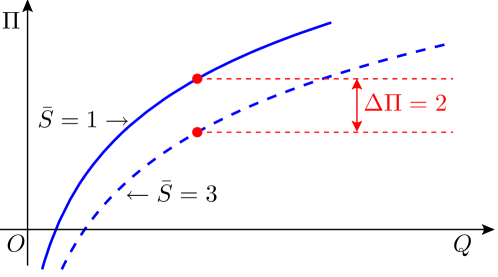
Figure 2: Two indifference curves of the same user type with two different expected payoffs, i.e., $\bar{S}=1$ and $\bar{S}=3$.

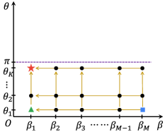
(a) $\theta_{1}<\theta_{K}<\pi$

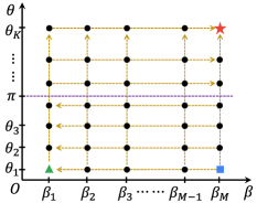
(b) $\theta_{1}<\pi<\theta_{K}$

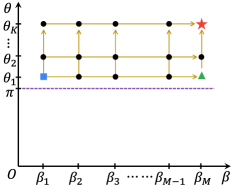
(c) $\pi<\theta_{1}<\theta_{K}$

Figure 3: Three market modes.

The slope of an indifference curve is called the marginal rate of substitution (MRS), which is the rate at which a consumer is ready to give up one good in exchange for another good, while maintaining the same level of satisfaction. In our problem, we denote the MRS of a type-$(\beta,\theta)$ user on a data cap $Q$ as

$$\sigma(Q,\beta,\theta)\triangleq\frac{\partial\Pi}{\partial Q}=-\left[\theta\beta+\pi(1-\beta)\right]\frac{\partial A(Q)}{\partial Q},$$ (16)

which depends on the user’s private information $(\beta,\theta)$ and the data cap $Q$. The MRS $\sigma(Q,\beta,\theta)$ indicates a type-$(\beta,\theta)$ user’s willingness-to-pay for an additional unit of data on a data cap $Q$. In the rest of the paper, we will use the three phrases “marginal rate of substitution”, “slope of the indifference curve”, and “willingness-to-pay” interchangeably.

4.2 User Ordering Based on Willingness-to-Pay

Without loss of generality, now we sort and index the ${KM}$ user types $(\beta_{m},\theta_{k})$ based on the corresponding willingness-to-pay $\sigma(Q,\beta_{m},\theta_{k})$ in an ascending order as follows:

$$\Lambda_{1}(Q),\ \Lambda_{2}(Q),\ ...,\ \Lambda_{KM}(Q),$$ (17)

where $\Lambda_{i}(Q)\triangleq\{\beta_{m},\theta_{k}\}$ for some $k$ and $m$. In this case, under the data cap $Q$, we have

$$\sigma(Q,\Lambda_{1})\leq\sigma(Q,\Lambda_{2})\leq...\leq\sigma(Q,\Lambda_{KM}).$$ (18)

Lemma 1.

The new user ordering in (17) does not depends on the data cap. That is, for any $Q\neq Q^{\prime}$, we have

$$\Lambda_{i}(Q)=\Lambda_{i}(Q^{\prime}),\ \forall\ 1\leq i\leq KM.$$ (19)

Lemma 1 indicates that the user ordering in (17) does not change, even though the value of $\sigma(Q,\Lambda_{i})$ would change with the data cap $Q$. Intuitively, this is because that a user’s willingness-to-pay $\sigma(Q,\Lambda_{i})$ in (16) has a separable structure between the user types (i.e., $\theta$ and $\beta$) and the data cap $Q$. The proof of Lemma 1 is given in Appendix A.

For notation simplicity, in the following, we will directly use $\Lambda_{i}$ to denote a user type under the ordering specified in (18), and denote $\phi_{i}=\{Q_{i},\Pi_{i}\}$ the contract item intended for the type-$\Lambda_{i}$ users.

To have a better understanding on the new user ordering, we use Fig. 3 to illustrate how $(\beta_{m},\theta_{k})$ maps to $\Lambda_{i}$. There are three different market modes depending on the relationship between the extreme valuations ($\theta_{1}$ and $\theta_{K}$) and the overage fee $\pi$, i.e., $\theta_{K}<\pi$ as in Fig. 3(a), $\theta_{1}<\pi<\theta_{K}$ as in Fig. 3(b), and $\pi<\theta_{1}$ as in Fig. 3(c). Specifically, the arrows in Fig. 3 point to the direction where the user’s MRS $\sigma(Q,\beta,\theta)$ increases, the blue square denotes the minimum willingness-to-pay user type-$\Lambda_{1}$, and the red star denotes the largest willingness-to-pay user type-$\Lambda_{KM}$. The following proposition summarizes the mapping from $(\beta_{m},\theta_{k})$ to $\Lambda_{1}$ and $\Lambda_{KM}$. The proof is given in Appendix A.

Proposition 2.

Under the three market modes, the type-$\Lambda_{1}$ and type-$\Lambda_{KM}$ users have their private information as follows:

$$\begin{cases}\Lambda_{1}=\{\beta_{M},\theta_{1}\},\Lambda_{KM}=\{\beta_{1},\theta_{K}\},&\text{if}\ \theta_{1}<\theta_{K}<\pi,\\ \Lambda_{1}=\{\beta_{M},\theta_{1}\},\Lambda_{KM}=\{\beta_{M},\theta_{K}\},&\text{if}\ \theta_{1}<\pi<\theta_{K},\\ \Lambda_{1}=\{\beta_{1},\theta_{1}\},\ \Lambda_{KM}=\{\beta_{M},\theta_{K}\},&\text{if}\ \pi<\theta_{1}<\theta_{K}.\end{cases}$$ (20)

Furthermore, the green triangles in Fig. 3 denote the smallest-payoff user type $\Lambda_{\epsilon}(Q,\Pi)$ given the contract item $(Q,\Pi)$, defined as follows

$$\Lambda_{\epsilon}(Q,\Pi)\triangleq\arg\min\limits_{\Lambda_{i}}\bar{S}(Q,\Pi,\Lambda_{i}).$$ (21)

Lemma 2 indicates that the smallest-payoff user type $\Lambda_{\epsilon}(Q,\Pi)$ does not change with data cap or subscription fee. Similar to Lemma 1, this is because the separable structure between the user types (i.e., $\theta$ and $\beta$) and the contract item (i.e., $Q$ and $\Pi$). For notation simplicity, we will use $\Lambda_{\epsilon}$ in the following. The proof of Lemma 2 is in Appendix A.

Lemma 2.

The smallest-payoff user defined in (21) does not depends on the data cap or the subscription fee, i.e.,

$$\Lambda_{\epsilon}(Q,\Pi)=\Lambda_{\epsilon}(Q^{\prime},\Pi^{\prime}),\ \forall(Q^{\prime},\Pi^{\prime})\neq(Q,\Pi).$$ (22)

Proposition 3 presents the mapping from $(\beta_{m},\theta_{k})$ to $\Lambda_{\epsilon}$. The proof is in Appendix A.

Proposition 3.

Under the three market modes, the type-$\Lambda_{\epsilon}$ user has the private information as follows:

$$\begin{cases}\Lambda_{\epsilon}=\{\beta_{1},\theta_{1}\},&\text{if}\ \theta_{1}<\theta_{K}<\pi,\\ \Lambda_{\epsilon}=\{\beta_{1},\theta_{1}\},&\text{if}\ \theta_{1}<\pi<\theta_{K},\\ \Lambda_{\epsilon}=\{\beta_{M},\theta_{1}\},&\text{if}\ \pi<\theta_{1}<\theta_{K}.\end{cases}$$ (23)

Next we study the necessary conditions for a contract to be feasible based on users’ willingness-to-pay.

4.3 Necessary Conditions

Lemmas 3 and 4 present two necessary conditions for a contract to be feasible (satisfying IC and IR conditions). The proofs are given in Appendix B.

Lemma 3.

For any feasible contract $\Phi(\mathcal{B},\Theta)$, $Q_{i}<Q_{j}$ if and only if $\ \Pi_{i}<\Pi_{j}$.

Lemma 4.

For any feasible contract $\Phi(\mathcal{B},\Theta)$, if $\sigma(Q,\Lambda_{i})>\sigma(Q,\Lambda_{j})$ for all $Q$, then $Q_{i}\geq Q_{j}$.

Lemma 3 reveals that a larger data cap corresponds to a higher subscription fee in the feasible contract, which is intuitive. Lemma 4 shows that a user with a stronger willingness-to-pay for the data cap deserves a larger data cap in the feasible contract. Next we provide a proof sketch for Lemma 4 to show the key insights.

Proof Sketch of Lemma 4.

We illustrate the key insights of Lemma 4 based on the contract plane in Fig. 4.

• For a type-$\Lambda_{j}$ user, we assume that the red dot in Fig. 4 is the contract item $\phi_{j}$ intended for this user type, and the red circle curve $l_{j}$ represents his indifference curve with a payoff equal to that of selecting $\phi_{j}$.

• For a type-$\Lambda_{i}$ user, the blue square curve $l_{i}$ is his indifference curve with a payoff equal to this user choosing the red dot contract item $\phi_{j}$ (not intended for his type).

It is obvious that $l_{i}$ is steeper than $l_{j}$; mathematically speaking, $\sigma(Q,\Lambda_{i})>\sigma(Q,\Lambda_{j})$ for all $Q$ (which is the condition in Lemma 4). That is, comparing with the type-$\Lambda_{j}$ users, the type-$\Lambda_{i}$ users have a stronger willingness-to-pay under any data cap. Moreover, as a user’s indifference curve shifts downward, his payoff increases because of the decreasing subscription fee.

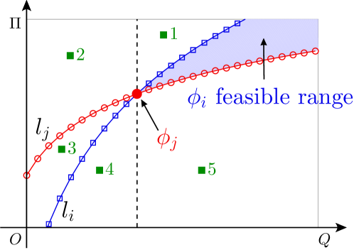
Figure 4: An illustration for Lemma 4.

Next we will show that to ensure the PIC condition $\phi_{i}\stackrel{{\scriptstyle{\tiny\text{IC}}}}{{\Longleftrightarrow}}\phi_{j}$, the contract item $\phi_{i}$ (intended for the type-$\Lambda_{i}$ users) must locate below (or on) the blue square curve $l_{i}$ and above (or on) the red circle curve $l_{j}$, i.e., in the blue region of Fig. 4. We prove this by contradiction. Assuming that this is not true, then we need to consider the following two scenarios:

• Scenario 1: The contract item $\phi_{i}$ is above the blue square curve $l_{i}$, such as the green squares labeled 1, 2, 3 in Fig. 4. In this case, the indifference curve $l_{i}$ for the type-$\Lambda_{i}$ should shift upward (with a decreasing payoff) to touch one of the three green squares. However, the type-$\Lambda_{i}$ user can achieve a higher payoff (comparing with selecting $\phi_{i}$) by selecting the red dot contract item $\phi_{j}$, which violates the PIC condition for the type-$\Lambda_{i}$ user.

• Scenario 2: The contract item $\phi_{i}$ is below the red circle curve ${l}_{j}$, such as the green squares labeled 4 and 5 in Fig. 4. In this case, the indifference curve $l_{j}$ for the type-$\Lambda_{j}$ user should shift downward (with an increasing payoff) to touch one of the three green squares. Therefore, the type-$\Lambda_{j}$ user can achieve a higher payoff by selecting the green square contract item $\phi_{i}$, which violates the PIC condition for the type-$\Lambda_{j}$ users.

The above discussion indicates that the contract item $\phi_{i}$ must locate in the blue area, which is on the right of the dash line. Thus $Q_{i}\geq Q_{j}$, as Lemma 4 implies.   

According to Lemma 3 and Lemma 4, we summarize the necessary conditions for a feasible contract as follows:

Theorem 1 (Necessary Conditions for Feasibility).

The feasible contract $\Phi(\mathcal{B},\Theta)$ has the following structure

$$\left\{\begin{aligned} &Q_{1}\leq Q_{2}\leq...\leq Q_{KM},\\ &\Pi_{1}\leq\Pi_{2}\leq...\leq\Pi_{KM}.\end{aligned}\right.$$ (24)

4.4 Sufficient Conditions

Next we derive the sufficient conditions for the feasible contract though the following two transitivity properties for Pairwise Incentive Compatibility (PIC) and Individual Rationality (IR). The proofs are given in Appendix C.

Lemma 5 (PIC-Transitivity).

Suppose the necessary conditions in Theorem 1 hold, then for any $i_{1}<i_{2}<i_{3}$, the following is true

$$\text{if}\ \phi_{i_{1}}\stackrel{{\scriptstyle{\tiny\text{IC}}}}{{\Longleftrightarrow}}\phi_{i_{2}}\text{ and }\phi_{i_{2}}\stackrel{{\scriptstyle{\tiny\text{IC}}}}{{\Longleftrightarrow}}\phi_{i_{3}},\text{ then }\phi_{i_{1}}\stackrel{{\scriptstyle{\tiny\text{IC}}}}{{\Longleftrightarrow}}\phi_{i_{3}}.$$ (25)

The above PIC transitivity property makes the contract problem (i.e., Problem 1) more tractable. It shows that we can reduce a total of ${KM(KM-1)/2}$ PIC conditions to a total of ${KM-1}$ PIC conditions for the neighbor user type pairs, i.e., $\phi_{i}\stackrel{{\scriptstyle{\tiny\text{IC}}}}{{\Longleftrightarrow}}\phi_{i+1},\ i=1,2,...,{KM-1}$.

We presents the IR transitivity in Lemma 6.

Lemma 6 (IR-Transitivity).

Suppose the necessary conditions in Theorem 1 and all PIC conditions hold, then the following is true,

$$\text{if }\phi_{\epsilon}\succcurlyeq 0,\text{ then }\phi_{i}\succcurlyeq 0,\ \forall\ i\neq\epsilon.$$

Recall that the user type-$\Lambda_{\epsilon}$, defined in (21), achieves the smallest payoff among all the user types for any given contract item. Lemma 6 implies that once we can guarantee all the PIC conditions, then we only need to further ensure that the IR constraint for the smallest-payoff type-$\Lambda_{\epsilon}$ users. This allows us to reduce a total of $KM$ IR conditions to one IR condition $\phi_{\epsilon}\succcurlyeq 0$.

Before we present the sufficient conditions for the feasible contract, we first introduce a user’s virtual payoff increment. Recall that $L(Q,\Lambda_{i})$ defined in (5) denotes the type-$\Lambda_{i}$ user’s virtual payoff. We define $\eta^{-}(\Lambda_{i},Q_{i},Q_{i-1})$ and $\eta^{+}(\Lambda_{i},Q_{i},Q_{i+1})$ as the type-$\Lambda_{i}$ user’s virtual payoff increments between selecting the contract item $\phi_{i}$ and the contract items intended for his neighbor user types (i.e., $\phi_{i-1}$ and $\phi_{i+1}$), as follows

$$\eta^{-}(\Lambda_{i},Q_{i},Q_{i-1})=L(Q_{i},\Lambda_{i})-L(Q_{i-1},\Lambda_{i}),$$ (26a)

$$\eta^{+}(\Lambda_{i},Q_{i},Q_{i+1})=L(Q_{i},\Lambda_{i})-L(Q_{i+1},\Lambda_{i}).$$ (26b)

Based on Lemmas 3$\sim$6, we derive the following sufficient conditions for a contract to be feasible.

Theorem 2 (Sufficient Conditions for Feasibility).

The contract $\Phi(\mathcal{B},\Theta)$ is feasible if all the following conditions hold,

1. $Q_{1}\leq Q_{2}\leq...\leq Q_{KM}$,

2. for $i=\epsilon$,

   $$\Pi_{\epsilon}\leq L(Q_{\epsilon},\Lambda_{\epsilon}),$$ (27)

3. for all $i=1,2,...,\epsilon-1$,

   $$\Pi_{i}\leq\Pi_{i+1}+\eta^{+}(\Lambda_{i},Q_{i},Q_{i+1}),$$ (28a)

   $$\Pi_{i}\geq\Pi_{i+1}-\eta^{-}(\Lambda_{i+1},Q_{i+1},Q_{i}).$$ (28b)

4. for all $i=\epsilon+1,\epsilon+2,...,{KM}$,

   $$\Pi_{i}\leq\Pi_{i-1}+\eta^{-}(\Lambda_{i},Q_{i},Q_{i-1}),$$ (29a)

   $$\Pi_{i}\geq\Pi_{i-1}-\eta^{+}(\Lambda_{i-1},Q_{i-1},Q_{i}),$$ (29b)

Now we discuss the intuitions of Theorem 2. Condition 1) satisfies the necessary conditions in Theorem 1. Condition 2) guarantees the IR condition for the type-$\Lambda_{\epsilon}$ users, i.e., $\phi_{\epsilon}\succcurlyeq 0$, which is sufficient for the IR conditions of all other user types according to Lemma 6. Condition 3) and Condition 4) guarantee the PIC condition for the neighbor user types, i.e., $\phi_{i}\stackrel{{\scriptstyle{\tiny\text{IC}}}}{{\Longleftrightarrow}}\phi_{i+1},\ \forall\ 1\leq i\leq{KM-1}$, which is sufficient for the global IC condition according to Lemma 5. Specifically, the inequality (28a) ensures that the type-$\Lambda_{i}$ user will not select the contract item $\phi_{i+1}$, i.e., $\bar{S}(\phi_{i},\Lambda_{i})\geq\bar{S}(\phi_{i+1},\Lambda_{i})$; the inequality (28b) ensures the type-$\Lambda_{i+1}$ user will not select the contract item $\phi_{i}$, i.e., $\bar{S}(\phi_{i+1},\Lambda_{i+1})\geq\bar{S}(\phi_{i},\Lambda_{i+1})$. Similar intuitions apply to (29).

So far we have derived the necessary and sufficient conditions for a feasible contract. Next we will analyze the optimality of the contract.

5 Contract Optimality

We will study the MNO’s optimal contract problem (i.e., Problem 1) based on the necessary and sufficient conditions for a feasible contract. To reveal the key insights, we will investigate the contract optimality in the following two steps.

• First, in Problem 2, we derive the MNO’s optimal prices $\{\Pi_{i}^{*}(\bm{Q}),1\leq i\leq{KM}\}$ given a feasible choice of data caps $\bm{Q}=\{Q_{i},1\leq i\leq KM\}$ where $Q_{1}\leq Q_{2}\leq...\leq Q_{KM}$.

• Second, in Problem 3, we substitute the optimal prices $\{\Pi_{i}^{*}(\bm{Q}),1\leq i\leq{KM}\}$ to the MNO’s profit function and derive the optimal data cap $\bm{Q}^{*}=\{Q_{i}^{*},1\leq i\leq{KM}\}$.

5.1 Optimal Pricing

In Problem 2, we compute the MNO’s optimal prices, denoted by $\{\Pi_{i}^{*}(\bm{Q}),1\leq i\leq{KM}\}$, given a feasible data cap allocation $\bm{Q}$, i.e., $Q_{1}\leq Q_{2}\leq...\leq Q_{KM}$. Note that the constraints (27), (29), and (28) are the sufficient conditions in Theorem 2. Hence the solution $\{\Pi_{i}^{*}(\bm{Q}),1\leq i\leq{KM}\}$ together with the given data cap $\bm{Q}$ must be a feasible contract.

Problem 2 (Optimal Prices).

$$\max\sum\limits_{i=1}^{KM}q(\Lambda_{i})\Big{[}\Pi_{i}+P(Q_{i},\Lambda_{i})-c\cdot U(Q_{i},\Lambda_{i})-J(Q_{i})\Big{]}$$ (30)

$$\ \textit{s.t. }\ (\ref{Equ: Sufficient IR u}),(\ref{Equ: Sufficient IC k<u}),(\ref{Equ: Sufficient IC k>u})$$

$$\ \textit{var. }\ \Pi_{i},1\leq i\leq{KM}.$$

Next we characterize the optimal prices $\{\Pi_{i}^{*}(\bm{Q}),1\leq i\leq{KM}\}$ in Theorem 3. The proof is given in Appendix D.

Theorem 3 (Optimal Pricing Policy).

Given a set of feasible data caps $\bm{Q}$ satisfying $Q_{1}\leq Q_{2}\leq...\leq Q_{KM}$. The optimal pricing policy for the MNO, denoted by $\{\Pi_{i}^{*}(\bm{Q}),1\leq i\leq{KM}\}$, is

$$\Pi^{*}_{i}(\bm{Q})=L\left(Q_{i},\Lambda_{i}\right), \text{if }i=\epsilon,$$ (31a)

$$\Pi^{*}_{i}(\bm{Q})=\Pi^{*}_{i+1}(\bm{Q})+\eta^{+}\left(\Lambda_{i},Q_{i},Q_{i+1}\right), \text{if }i<\epsilon,$$ (31b)

$$\Pi^{*}_{i}(\bm{Q})=\Pi^{*}_{i-1}(\bm{Q})+\eta^{-}\left(\Lambda_{i},Q_{i},Q_{i-1}\right), \text{if }i>\epsilon.$$ (31c)

Comparing Theorem 2 and Theorem 3, we notice that, given a set of feasible data caps $\bm{Q}$, the MNO should charge the highest prices satisfying the IC and IR conditions.

Next we further study the MNO’s optimal data caps $\bm{Q}$ based on the optimal prices $\{\Pi_{i}^{*}(\bm{Q}),1\leq i\leq{KM}\}$ in (31).

5.2 Optimal Data Caps

For notation simplicity, we first introduce the concept of virtual payoff difference. For a given data cap $Q$, the virtual payoff differences between the type-$\Lambda_{i}$ user and his neighbor user types (i.e., $\Lambda_{i-1}$ and $\Lambda_{i+1}$) are defined as

$$\rho^{-}_{i}(Q)\triangleq L(Q,\Lambda_{i})-L(Q,\Lambda_{i-1}),$$ (32a)

$$\rho^{+}_{i}(Q)\triangleq L(Q,\Lambda_{i})-L(Q,\Lambda_{i+1}).$$ (32b)

We substitute the optimal prices (31) derived in Theorem 3 into the objective function of Problem 2, and write the MNO’s objective function (i.e., the total profit) as follows:

$$\sum_{i=1}^{KM}G_{i}\left(Q_{i}\right),$$ (33)

where $G_{i}(\cdot)$ is given by (34), and $h^{i}=\textstyle\sum_{t=1}^{i-1}q(\Lambda_{t})$ and $h_{i}=\sum_{t=i+1}^{KM}q(\Lambda_{t})$ are two constants related to the distribution of the user types. Thus we get the following optimization problem over the $KM$ data caps.

$$G_{i}(Q)=\left\{\begin{aligned} &q(\Lambda_{i})V(Q,\Lambda_{i})-q(\Lambda_{i})\left[c\cdot U(Q,\Lambda_{i})+J(Q)\right],\qquad\qquad\qquad\qquad\quad\ \ \text{if }i\in\{1,KM\},\\ &q(\Lambda_{i})V(Q,\Lambda_{i})+h^{i}\rho^{-}_{i}(Q)-q(\Lambda_{i})\left[cU(Q,\Lambda_{i})+J(Q)\right],\qquad\qquad\quad\ \text{if }i\in\{2,3,...,\epsilon-1\},\\ &q(\Lambda_{i})V(Q,\Lambda_{i})+h^{i}\rho^{-}_{i}(Q)+h_{i}\rho^{+}_{i}(Q)-q(\Lambda_{i})\left[cU(Q,\Lambda_{i})+J(Q)\right],\ \text{if }i={\epsilon},\\ &q(\Lambda_{i})V(Q,\Lambda_{i})+h_{i}\rho^{+}_{i}(Q)-q(\Lambda_{i})\left[cU(Q,\Lambda_{i})+J(Q)\right],\qquad\qquad\quad\ \ \text{if }i\in\{\epsilon+1,\epsilon+2,...,KM-1\},\end{aligned}\right.$$ (34)

Problem 3 (Optimal Data Caps).

$$\max\sum\limits_{i=1}^{KM}G_{i}\left(Q_{i}\right)$$ (35a)

$$\ \textit{s.t. }\ \ Q_{1}\leq Q_{2}\leq...\leq Q_{KM}\leq D$$ (35b)

$$\quad\quad\ Q_{i}\in\mathbb{N},\ \forall\ i\in\{1,2,...,KM\}$$ (35c)

$$\ \textit{var. }\ Q_{i},1\leq i\leq{KM}.$$ (35d)

Problem 3 is a nonlinear integer programming with two special structures. First, the objective function has a separable structure over each decision variable $Q_{i}$. Second, the decision variables are monotonic. Moreover, the convexity of Problem 3 depends on all user types $\Lambda_{i}$ for all $1\leq i\leq KM$ and the corresponding distribution $q(\Lambda_{i})$ for all $1\leq i\leq KM$.

In previous literature (e.g., [33, 34, 35, 36]), the commonly used approach to solving Problem 3 is monotonicity relaxation. The main idea is to first relax the monotonicity constraints (35b) and maximize each $G_{i}(\cdot)$ over the corresponding decision variable $Q_{i}$. If the solution obtained under the relaxation violates the monotonicity constraints (35b), then one needs to adjust the solution according to the algorithm proposed in [33] to become feasible. We refer interested readers to Appendix E for more details. In general, the monotonicity relaxation approach is very efficient, since it only needs to deal with several single-variable optimization problems. However, the adjusted solution is only a locally optimal solution when the problem is not convex [1]. Moreover, it is difficult to analytically characterize the sub-optimality gap of the solution. To obtain the globally optimal solution of Problem 3 efficiently, in Section 5.3, we will propose the Dynamic Quota Allocation Algorithm, which is one of the major contributions in this paper.

5.3 Dynamic Quota Allocation (DQA) Algorithm

5.3.1 Basic Idea

The basic idea of the DQA Algorithm comes from dynamic programming, i.e., breaking the original problem down into simpler sub-problems in a recursive manner [37]. Specifically, we will decompose Problem 3 by utilizing the separability of objective (35a) and the monotonicity constraints (35b). Next we introduce how to define the proper sub-problems.

5.3.2 Level-($n,q$) Subproblem

In the DQA Algorithm, we refer to Problem 4 as the level-($n,q$) sub-problem of Problem 3. Basically, the level-($n,q$) sub-problem focuses on the optimal data caps for the smallest $n$ user types (i.e., type-$1$ to type-$n$, where $1\leq n\leq KM$) under the data cap upper bound $q$ ($0\leq q\leq D$). Recall that there are a total of $KM$ types of users and $D$ is users’ maximal possible monthly data demand. The special case of the level-($KM,D$) sub-problem is equivalent to Problem 3, since the MNO does not need to offer any data cap larger than $D$.

Problem 4 (Level-$(n,q)$ Sub-problem).

Given $1\leq n\leq KM$ and $0\leq q\leq D$, the level-$(n,q)$ sub-problem is

$$H(n,q)\triangleq\arg\max\ \sum_{i=1}^{n}G_{i}(Q_{i})$$ (36a)

s.t. $$Q_{1}\leq Q_{2}\leq...\leq Q_{n}\leq q$$ (36b)

$$Q_{i}\in\mathbb{N},\ \forall\ i\in\{1,2,...,n\}$$ (36c)

var: $$Q_{i},1\leq i\leq n.$$ (36d)

Here we denote $H(n,q)$ and $\bm{Q}^{\star}(n,q)=\{Q^{\star}_{i}(n,q),1\leq i\leq n\}$ as the optimal value and the optimal solution of the level-($n,q$) sub-problem (36), respectively. Since the level-($KM,D$) sub-problem is equivalent to Problem 3, we have

• The optimal value of Problem 3 is $H(KM,D)$.

• The optimal data caps in Problem 3 is $\bm{Q}^{\star}(KM,D)$, i.e., $Q_{i}^{*}=Q_{i}^{\star}(KM,D)$ for all $1\leq i\leq KM$.

In the following, we will show that if we know $H(n,q)$ for all $1\leq n\leq KM$ and $0\leq q\leq D$, then we can directly find $\bm{Q}^{\star}(KM,D)$. To present this connection clearly, we first introduce some properties of $H(n,q)$ in Propositions 4 and 5. The proofs are given in Appendix F.

Proposition 4.

For any $2\leq n\leq KM$ and $0\leq q\leq D$, $H(n,q)$ has the following recursive relation

$$H(n,q)=\max\limits_{x\in\mathbb{N}}\ H(n-1,x)+G_{n}(x)$$ (37a)

s.t. $$x\leq q.$$ (37b)

The proof of Proposition 4 follows the definition of the level-($n,q$) sub-problem in (36).

Proposition 5.

Given any $n\in\{1,2,...,KM\}$, we have

• Function $H(n,q)$ is non-decreasing in the data cap $q$.

• There exists a critical point $\hat{q}_{n}$ such that $H(n,q)$ does not change for any $q\geq\hat{q}_{n}$.

The intuitions behind Proposition 5 are two-fold.

• First, the non-decreasing property of $H(n,q)$ results from the constraints (36b). Mathematically, $q$ in (36b) defines the domain upper bound of the level-($n,q$) sub-problem. That is, a larger $q$ in (36b) corresponds to a larger feasible domain, hence a no smaller optimal value $H(n,q)$.

• Second, $H(n,q)$ will not increase in $q$ anymore if the optimal solution of the level-($n,q$) sub-problem is smaller than the domain upper bound $q$. Basically, $\hat{q}_{n}$ equals to the $n$-th element of the optimal solution $\bm{Q}^{\star}(n,D)$ for the level-($n,D$) sub-problem, i.e.,

  $$\hat{q}_{n}=Q_{n}^{\star}(n,D).$$ (38)

Based on the recursiveness shown in Propositions 4 and the critical points $\{\hat{q}_{i},1\leq i\leq KM\}$ shown in Proposition 5, we are able to find the optimal solution of the level-($KM,D$) sub-problem (which is the same as Problem 3) according to Theorem 4. The proof is given in Appendix F.

Theorem 4.

The optimal solution $\{Q^{\star}_{i}(KM,D),1\leq i\leq KM\}$ of the level-($KM,D$) sub-problem is

$$Q_{i}^{\star}(KM,D)=\begin{cases}\hat{q}_{i},&\text{if }i=KM,\\ \min\{\hat{q}_{i},Q_{i+1}^{\star}(KM,D)\},&\text{if }i<KM.\end{cases}$$ (39)

We elaborate Theorem 4 as follows:

• For $i=KM$, according to (38), we know that the optimal data cap $Q_{KM}^{\star}(KM,D)$ is the same as the critical point mentioned in Proposition 5, i.e., $Q_{KM}^{\star}(KM,D)=\hat{q}_{KM}$.

• For the other user types, i.e., $i<KM$, according to (37b) in Proposition 4, the optimal data cap $Q_{i}^{\star}(KM,D)$ is the smaller one between the critical point $\hat{q}_{i}$ and the optimal data cap for the next user type $Q_{i+1}^{\star}(KM,D)$.

Here we want to emphasize that (39) only needs the $KM$ critical points $\{\hat{q}_{i},1\leq i\leq KM\}$, which can be easily obtained from the table of $H(n,q)$ for all $1\leq n\leq KM$ and $0\leq q\leq D$. In Appendix G, we provide a numerical example to demonstrate how to find the optimal data caps based on the table $H(n,q)$.

The remaining question is how to compute the table of $H(n,q)$. We solve this problem by proposing the DQA Algorithm next.

Input : All user types $\Lambda_{i}$ and the distribution $q(\Lambda_{i})$.

Output :  $H(n,q)$ for all $1\leq n\leq KM$ and $0\leq q\leq D$.

1 Initial $H(n,q)=0,\ \forall\ 1\leq n\leq KM$ and $0\leq q\leq D$.

2 for $n=1$ to $KM$  do

3       for $q=0$ to $D$ do

4             if $n=1$ then

5                   $H(n,q):=\max\limits_{x\leq q}G_{n}(x)$.

6                  

7            else

8                   $H(n,q):=\arg\max\limits_{x\leq q}H(n-1,x)+G_{n}(x)$.

9                  

10            

11      

Algorithm 1 Dynamic Quota Allocation (DQA)

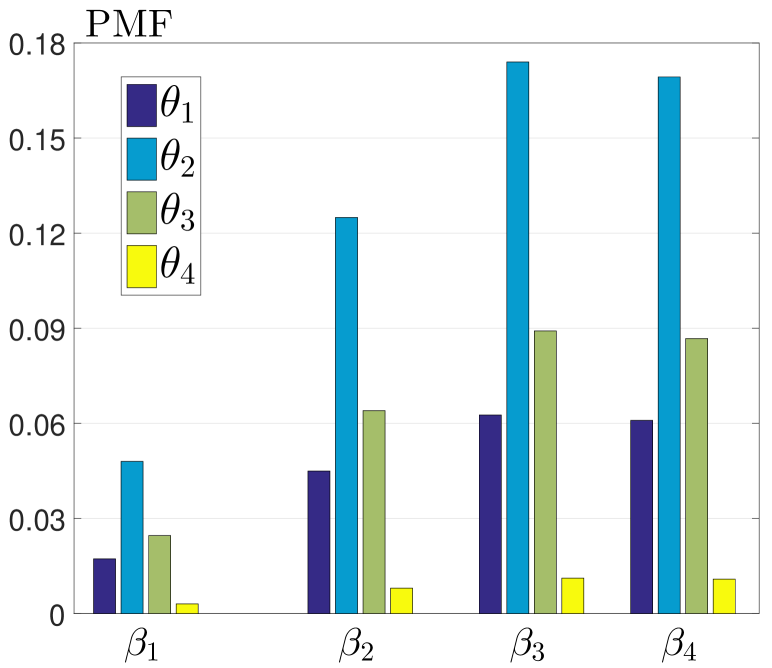
Figure 5: User type distribution.

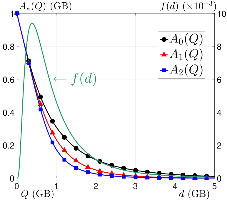
Figure 6: $f(d)$ vs. $d$ and $A_{\kappa}(Q)$ vs. $Q$.

Figure 7: Structure of optimal contract.

5.3.3 DQA Algorithm

To compute $H(n,q)$ efficiently, we need to take the advantage of its recursiveness (in Proposition 4) again. The detailed process is shown in Algorithm 1. Specifically, the input of Algorithm 1 includes all of the user types $\Lambda_{i}$ and the corresponding distribution (probability mass function) $q(\Lambda_{i})$. The output of this algorithm is the table of $H(n,q)$ for all $1\leq n\leq KM$ and $0\leq q\leq D$. In Line 5, we compute $H(1,q)$ for all $q\in\{0,1,2,...,D\}$. In Line 7, we compute $H(n,q)$ for all $n\geq 2$ by utilizing the recursiveness in Proposition 4.

Algorithm 1 has a computational complexity of $O(KM|\mathcal{Q}|^{2})$, where $KM$ is the number of user types and the set $\mathcal{Q}$ consists of all the possible data caps. It is actually quite efficient in the implementation process, since the MNO usually set the data caps to be the nearest hundreds of MB (e.g., 100MB, 500MB, and 1GB). For example, suppose that the maximal data demand is $D=10$GB (which is large enough in most cases). If the MNO would optimize the data cap with 1MB as the minimal unit, then there are a total of $|\mathcal{Q}|=10001$ possible data caps (i.e., $\mathcal{Q}=\{$0MB, 1MB, 2MB, 3MB,…, 10000MB$\}$) to be considered in this algorithm. If the MNO would optimize the data cap with 100MB as the minimal unit, then there are only a total of $|\mathcal{Q}|=101$ possible data caps (i.e., $\mathcal{Q}=\{$0MB, 100MB, 200MB, 300MB,…, 10000MB$\}$). Hence the algorithm is efficient in the implementation progress.

So far, we have completely solved the optimal contract. Next we evaluate the proposed multi-dimensional contract.

6 Numerical Results

We evaluate the performance of the optimal contract based on some empirical data. Specifically, we first illustrate the optimal contract structure in Section 6.1, then investigate how the price discrimination and the time flexibility affect the MNO’s profit and users’ payoffs in Section 6.2.

6.1 Optimal Contract

Next we introduce the estimated user types, data demand distribution, and the MNO’s cost. Then we illustrate the optimal contract structure.

Estimated User Types: According to the market survey results (based on over two thousand users of mainland China) in [8], a large proportion of users’ data valuations $\theta$ is within the interval of $[15,65]$ (in RMB/GB); most people would like to shrink approximately $70\%\sim 100\%$ overage data consumption through alternative networks ($\beta$ value). We follow [26] by using the $k$-means clustering method to partition the empirical data valuation $\theta$ into four clusters with mean values $\Theta=\{16.2,36.1,61.9,96.3\}$, and partition the empirical network substitutability $\beta$ into four clusters with mean value $\mathcal{B}=\{0.51,0.71,0.84,0.95\}$. Therefore, we consider a total of $KM=16$ user types, and the corresponding distribution extracted from empirical data is shown in Fig. 7.

Data Demand Distribution: We set the minimum data unit as $1$MB. Following the data analysis results in [22, 23], we suppose that users’ monthly data demand follows a truncated log-normal distribution over the support of $[0,10^{4}]$ with a mean $\bar{d}=10^{3}$, i.e., the average data demand $\bar{d}=1$GB and the maximal potential data demand $D=10$GB [8]. Fig. 7 shows the PMF $f(d)$ and the expected overage data consumption $A_{\kappa}(Q)$ under different data mechanisms $\kappa\in\{0,1,2\}$, which indicates that $A_{0}(Q)\geq A_{1}(Q)\geq A_{2}(Q)$ for any $Q$.

MNO’s Cost: As mentioned in (10) of Section 3.3, we take account of the capacity cost and the operational cost for the MNO. To be consistent with our previous work [8], we suppose that the capacity cost takes a linear form, i.e., $J(Q)=z\cdot Q$, where $z$ represents the MNO’s marginal capacity cost. In addition, $c$ represents the MNO’s marginal operational cost. Next we will vary the two parameters (i.e., $c$ and $z$) to illustrate their effects on the optimal contract and the corresponding MNO profit and user payoff.

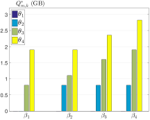
(a) Data caps under $\kappa=0$.

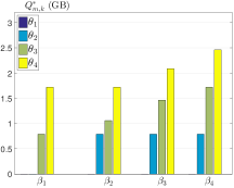
(b) Data caps under $\kappa=1$.

(c) Data caps under $\kappa=2$.

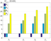
(d) Subscription fees under $\kappa=0$.

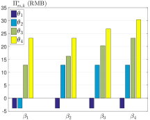
(e) Subscription fees under $\kappa=1$.

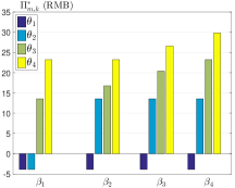
(f) Subscription fees under $\kappa=2$.

Figure 8: Optimal contract under the three data mechanisms $\kappa\in\{0,1,2\}$.

Furthermore, we use the per-unit fee in the telecommunication market of China, i.e., $\pi=30$ RMB/GB. Based on the above setting, we will evaluate the optimal contract in the following three steps.

6.1.1 Contract Structure

We take the data mechanism $\kappa=1$ as example to visualize the contract structure based on the users’ types.

Fig. 7 shows some properties of the optimal contract item for each user type, given the MNO’s cost $c=5$RMB/GB, $z=0.9$RMB/GB. Specifically, the markers represent all the user types $\Lambda_{i}=(\beta_{m},\theta_{k})$, each of which corresponds to a network substitutability $\beta_{m}$ and a data valuation $\theta_{k}$ in the horizontal and vertical axis, respectively. Moreover, the arrows point to the non-decreasing direction of users’ willingness-to-pay as defined in (17). The markers of the same shape and color represent that the corresponding users types have the same contract item (i.e., pooling contract). Therefore, the optimal contract contains seven different contract items for a total of $KM=16$ types of users.

6.1.2 Impact of Data Mechanisms

Next we compare the optimal contract under different data mechanisms $\kappa\in\{0,1,2\}$.

Fig. 8 plots the optimal data caps (i.e., Figs. 8(a), 8(b), 8(c)) under the three data mechanisms and the corresponding subscription fees (i.e., Figs. 8(d), 8(e), 8(f)). We have the following observations:

• For all three data mechanisms, the optimal contract offers some low valuation users (e.g., $\Lambda_{1}$) a zero data cap (e.g., pure usage-based plan in Fig. 8(a)), together with a negative price (e.g., the five negative bars in Fig. 8(d)). The pure usage-based plan reduces the MNO’s capacity cost due to the zero data cap. Meanwhile, the negative price serves as a price discount, which ensures the subscription of these users (still satisfying the IR condition).

• For each data mechanism $\kappa$, the optimal contract tends to offer the users who have small $\beta$ values hence poor alternative network choices (e.g., the type-$(\beta_{1},\theta_{3})$ users) a small data cap (e.g., 0.9GB in Fig. 8(a)) together a low subscription fee (e.g., 12RMB in Fig. 8(d)). As a result, these users will end up paying a lot of overage fee. However, the optimal contract offers the users who have high $\beta$ values hence good alternative network choices (e.g., the type-$(\beta_{4},\theta_{4})$ users) a large data cap (e.g., 2.8GB in Fig. 8(a)) together with a high subscription fee (e.g., 30RMB in Fig. 8(d)).

• Under the optimal contract, the better time flexibility (i.e., a larger value of $\kappa$) enables the MNO to offer a smaller data cap for the same type of users. For example, the optimal data cap for type-$(\beta_{4},\theta_{4})$ users is 2.8GB, 2.5GB, and 2.2GB in Fig. 8(a), 8(b), and 8(c), respectively. The MNO reduces its capacity cost by offering a better time flexibility (i.e., $\kappa=0\rightarrow 1\rightarrow 2$).

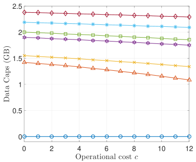
(a) Optimal data caps.

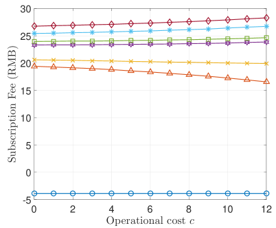
(b) Optimal subscripton fees.

Figure 9: Impact of MNO’s operational cost $c$.

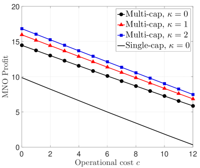
(a) MNO’s profit.

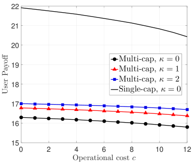
(b) All users’ expected payoff.

Figure 10: Impact of the MNO’s operational cost $c$.

6.1.3 Impact of MNO’s Costs

We take the data mechanism $\kappa=1$ as an example to investigate how the MNO’s costs (i.e., both $c$ and $z$) affect the optimal contract items.

Fig. 10 shows the impact of the MNO’s operational cost $c$. Specifically, there are a total of seven different contract items in the optimal contract. The seven curves in Fig. 9(a) represent the different data caps. We note that overall the optimal data caps (except the zero cap) decreases as the MNO’s operational cost increases. Fig. 9(b) plots the corresponding subscription fees versus the MNO’s operational cost. We find that

• The subscription fee of the zero-cap contract item (i.e., the bottom blue circle curve in Fig. 9(b)) does not change in the operation cost $c$. This results from the individual rationality condition as in (31a).

• The subscription fees of small-cap contract items (e.g., the orange triangle and yellow cross curves in Fig. 9(b)) decrease as the MNO’s costs increase. While the subscription fees of the large-cap contract items (the remaining curves) increase in the MNO’s costs. Therefore, the large-cap contract items become less economical to the users (in terms of the average price $\Pi/Q$) as the MNO’s costs increase. This means that a profit-maximizing MNO tends to compensate its operational cost by charging those users who are willing to pay for the large-cap contract items.

We also investigate the impact of the MNO’s capacity cost $z$. The insights are similar to those from Fig. 10. We refer interested readers to Appendix H for more details.

6.2 Impact of Price Discrimination and Time Flexibility

We evaluate the effect of the price discrimination and the time flexibility on the MNO’s profit and users’ payoffs.

We consider four scenarios as shown in Table IV. Scenario (i) represents the benchmark single-cap scheme under the traditional data mechanism $\kappa=0$ (studied in our previous work [8]). Scenarios (ii), (iii), and (iv) represent the multi-cap scheme under different data mechanisms (studied in this paper).

TABLE IV: Four scenarios.

Scenario	Multi-cap or Single-cap	Data Mechanism
(i)	Single	$\kappa=0$
(ii)	Multiple	$\kappa=0$
(iii)	Multiple	$\kappa=1$
(iv)	Multiple	$\kappa=2$

Fig. 10 plots the MNO’s profit and user’s payoffs in the four scenarios under different operational cost $c$.

• Fig. 10(a) plots MNO’s profits in the four scenarios. Overall, the MNO’s profits decrease in its operational cost $c$. By comparing the single-cap traditional pricing benchmark and the multi-cap traditional pricing scheme, we note that the price discrimination under our optimal contract can significantly increase the MNO’s profit (180% on average). By comparing the three multi-cap curves, we find that the MNO obtains a higher profit under a more time-flexible data mechanism. Specifically, compared with Scenario (ii) (i.e., the black circle curve), MNO’s profits increases by 15% on average in Scenario (iii) (i.e., the red triangle curve) and 25% on average in Scenario (iv) (i.e., blue square curve). This implies that under the multi-cap scheme, offering a better time flexibility can further improve the MNO’s profit.

• Fig. 10(b) plots the users’ total expected payoff in four scenarios. First, we observe that users’ payoff decreases in the MNO’s operational cost. By comparing the single-cap traditional pricing benchmark and the multi-cap traditional pricing scheme, we notice that the price discrimination under our optimal contract reduces users’ expected payoff (23% on average), which means that the MNO captures more consumer surplus through the price discrimination. Comparing the three multi-cap schemes, we find that the time-flexible data mechanisms can improve the users’ payoff. Specifically, compared with Scenario (ii) (i.e., the circle curve), users’ payoff increases by 5.1% on average in Scenario (iii) (i.e., the triangle curve) and 8.2% on average in Scenario (iv) (i.e., square curve).

We also evaluate the performance under different capacity cost $z$, which leads to similar insights. We refer interested readers to Appendix H for more details. Furthermore, we also evaluate the impact of the number of user types on the optimal contract performance. Due to page limit, we refer interested readers to Appendix I for more details.

7 Conclusion and Future Works

In this paper we studied how the MNO optimizes its multi-cap data plans under the time-flexible data mechanisms. Specifically, we consider an asymmetric information scenario, where each use is associated with two-dimensional private information, i.e., his data valuation and network substitutability. We formulate the MNO’s optimal multi-cap design as a multi-dimensional contract problem and derive the optimal contract under different data mechanisms. Our analysis revealed that the slope of a user’s indifference curve on the contract plane corresponds to his willingness-to-pay, and the feasible contract (satisfying IC and IR conditions) would offer a larger data cap to the user with the stronger willingness-to-pay. Moreover, we proposed an efficient algorithm to solve the contract problem optimally.

In the future, we have two directions to extend the results of this paper.

• First, we will collect more empirical data related to users’ data demand distributions and try to relax the current homogeneous assumption of the data demand distribution. This will lead to a new contract problem with three-dimensional private information, which will be much more challenging to solve.

• Second, we will consider the competitive market. So far we have shown that the time flexibility increases the MNO’s profit and users’ payoffs under the multi-cap scheme, it is still necessary to analyze the role of price discrimination and time flexibility on MNOs’ market competition. This will build upon our previous analysis of the competitive market under the single-cap scheme.

Zhiyuan Wang received the B.S. degree from Southeast University, Nanjing, China, in 2016. He is currently working toward the Ph.D. degree with the Department of Information Engineering, The Chinese University of Hong Kong, Shatin, Hong Kong. His research interests include the field of network economics and game theory, with current emphasis on smart data pricing and mobile edge computing. He is the recipient of the Hong Kong PhD Fellowship.

Lin Gao (S’08-M’10-SM’16) is an Associate Professor with the School of Electronic and Information Engineering, Harbin Institute of Technology, Shenzhen, China. He received the Ph.D. degree in Electronic Engineering from Shanghai Jiao Tong University in 2010. His main research interests are in the area of network economics and games, with applications in wireless communications and networking. He received the IEEE ComSoc Asia-Pacific Outstanding Young Researcher Award in 2016.

Jianwei Huang (F’16) is a Presidential Chair Professor and Associate Dean of the School of Science and Engineering, The Chinese University of Hong Kong, Shenzhen. He is also a Professor in the Department of Information Engineering at The Chinese University of Hong Kong. He is the co-author of 9 Best Paper Awards, including IEEE Marconi Prize Paper Award in Wireless Communications 2011. He has co-authored six books, including the textbook on “Wireless Network Pricing”. He has served as the Chair of IEEE Technical Committee on Cognitive Networks and Technical Committee on Multimedia Communications. He has been an IEEE ComSoc Distinguished Lecturer and a Thomson Reuters Highly Cited Researcher.

Appendix A

Proof of Lemma 1.

We prove this lemma by showing that if $\sigma(Q,\Lambda_{i})<\sigma(Q,\Lambda_{j})$, then $\sigma(Q^{\prime},\Lambda_{i})<\sigma(Q^{\prime},\Lambda_{j})$ for any $i,j\in\{1,2,...,KM\}$ and any $Q^{\prime}\neq Q$.

In this paper, we take into account two-dimensional user type. For a type-$\Lambda_{i}$ user, we denote $\beta^{i}$ and $\theta^{i}$ as his network substitutability and data valuation, respectively. That is, $\Lambda_{i}=\{\beta^{i},\theta^{i}\}$. Similarly, we have $\Lambda_{j}=\{\beta^{j},\theta^{j}\}$ for the type-$\Lambda_{j}$ user.

Recall that the user’s willingness-to-pay $\sigma(Q,\beta,\theta)$ is

$$\sigma(Q,\beta,\theta)=-\left[\theta\beta+\pi(1-\beta)\right]\frac{\partial A(Q)}{\partial Q},$$ (40)

which has a separable structure between user’s private information $(\beta,\theta)$ and the data cap $Q$. Therefore, $\sigma(Q,\Lambda_{i})<\sigma(Q,\Lambda_{j})$ implies that

$$-\left[\theta^{i}\beta^{i}+\pi(1-\beta^{i})\right]\frac{\partial A(Q)}{\partial Q}<$$ (41)

$$\qquad\qquad\qquad\qquad-\left[\theta^{j}\beta^{j}+\pi(1-\beta^{j})\right]\frac{\partial A(Q)}{\partial Q},$$

which means that

$$\textstyle\theta^{i}\beta^{i}+\pi(1-\beta^{i})<\theta^{j}\beta^{j}+\pi(1-\beta^{j}).$$ (42)

Multiply both sides of (42) by $-\frac{\partial A(Q^{\prime})}{\partial Q}$, we obtain

$$\textstyle-\left[\theta^{i}\beta^{i}+\pi(1-\beta^{i})\right]\frac{\partial A(Q^{\prime})}{\partial Q}<-\left[\theta^{j}\beta^{j}+\pi(1-\beta^{j})\right]\frac{\partial A(Q^{\prime})}{\partial Q},$$ (43)

which implies that $\sigma(\Lambda_{i},Q^{\prime})<\sigma(\Lambda_{j},Q^{\prime})$.   

Proof of Proposition 2.

We prove this proposition based on Lemma 1.

Recall that we consider a set $\Theta=\{\theta_{k}:1\leq k\leq{K}\}$ of $K$ data valuation types and a set $\mathcal{B}=\{\beta_{m}:1\leq m\leq{M}\}$ of $M$ network substitutability types. According to the proof of Lemma 1, we find that the new user order (based on their willingness-to-pay) only depends on the order of

$$\theta\beta+\pi(1-\beta)=\pi+(\theta-\pi)\beta.$$ (44)

The expression in (44) monotonically increases in $\theta$. However, it increases in $\beta$ if $\theta>\pi$ and decreases in $\beta$ if $\theta<\pi$. Therefore, we have three cases depending on the relation between $\pi$, $\theta_{1}$, and $\theta_{K}$.

• Fig. 3(a): The case of $\theta_{K}<\pi$ corresponds to $\Lambda_{1}=\{\beta_{M},\theta_{1}\}$ and $\Lambda_{KM}=\{\beta_{1},\theta_{K}\}$.

• Fig. 3(b): The case of $\theta_{1}<\pi<\theta_{K}$ corresponds to $\Lambda_{1}=\{\beta_{M},\theta_{1}\}$ and $\Lambda_{KM}=\{\beta_{M},\theta_{K}\}$.

• Fig. 3(c): The case of $\pi<\theta_{1}$ corresponds to $\Lambda_{1}=\{\beta_{1},\theta_{1}\}$ and $\Lambda_{KM}=\{\beta_{M},\theta_{K}\}$.

 

Proof of Lemma 2.

We prove this lemma together with Proposition 3 based on the user’s payoff. Recall that the type-$(\beta,\theta)$ user’s payoff is

$$\bar{S}(Q,\Pi,\beta,\theta)=\theta\left[\bar{d}-\beta A(Q)\right]-\pi(1-\beta)A(Q)-\Pi.$$ (45)

Take the derivative of (45) with respect to the user’s data valuation $\theta$, and we obtain

$$\frac{\partial\bar{S}(Q,\Pi,\beta,\theta)}{\partial\theta}=\bar{d}-\beta A(Q)\geq 0,\ \forall\ Q,$$ (46)

which means that the user’s payoff increases in the data valuation $\theta$.

Take the derivative of (45) with respect to the user’s network substitutability $\beta$, and we obtain

$$\frac{\partial\bar{S}(Q,\Pi,\beta,\theta)}{\partial\beta}=\left[\pi-\theta\right]A(Q),$$ (47)

which means that the user’s payoff decreases in $\beta$ if $\theta<\pi$ and increases in $\beta$ if $\theta>\pi$.

Therefore, we have three cases depending on the relation between $\pi$, $\theta_{1}$, and $\theta_{K}$.

• Fig. 3(a): The case of $\theta_{1}<\theta_{K}<\pi$ corresponds to $\Lambda_{\epsilon}=\{\beta_{1},\theta_{1}\}$.

• Fig. 3(b): The case of $\theta_{1}<\pi<\theta_{K}$ corresponds to $\Lambda_{\epsilon}=\{\beta_{1},\theta_{1}\}$.

• Fig. 3(c): The case of $\pi<\theta_{1}$ corresponds to $\Lambda_{\epsilon}=\{\beta_{M},\theta_{1}\}$.

Now we have proved the independence of $\Lambda_{\epsilon}$ on the contract item $(Q,\Pi)$ in Lemma 2 and the mapping relation in Proposition 3.   

Appendix B

Proof of Lemma 3.

We prove this lemma based on the IC condition in Definition 2.

First, we prove that if $Q_{i}<Q_{j}$, then $\Pi_{i}<\Pi_{j}$. For any feasible contract, we have the following IC condition for the type-$\Lambda_{i}$ user

$$L(Q_{i},\Lambda_{i})-\Pi_{i}\geq L(Q_{j},\Lambda_{i})-\Pi_{j},$$ (48)

which is equivalent to

$$\Pi_{i}-\Pi_{j}\leq L(Q_{i},\Lambda_{i})-L(Q_{j},\Lambda_{i}).$$ (49)

Since $Q_{i}<Q_{j}$, we have $L(Q_{i},\Lambda_{i})-L(Q_{j},\Lambda_{i})<0$, which implies that $\Pi_{i}<\Pi_{j}$.

Second, we prove that if $\Pi_{i}<\Pi_{j}$, then $Q_{i}<Q_{j}$. For any feasible contract, we have the following IC condition for the type-$\Lambda_{j}$ user:

$$L(Q_{j},\Lambda_{j})-\Pi_{j}\geq L(Q_{i},\Lambda_{j})-\Pi_{i},$$ (50)

which is equivalent to

$$L(Q_{j},\Lambda_{j})-L(Q_{i},\Lambda_{j})\geq\Pi_{j}-\Pi_{i}.$$ (51)

Since $\Pi_{j}>\Pi_{i}$, we have $L(Q_{j},\Lambda_{j})-L(Q_{i},\Lambda_{j})>0$, which implies that that $Q_{j}>Q_{i}$.   

Proof of Lemma 4.

We prove the lemma by contradiction. Assume that the lemma is not true and there exist $\sigma(Q,\Lambda_{i})>\sigma(Q,\Lambda_{j})$ and $Q_{i}<Q_{j}$ in a feasible contract.

According to the PIC condition in Definition 3, for the type-$\Lambda_{i}$ and type-$\Lambda_{j}$ users, we have

$$L(Q_{i},\Lambda_{i})-\Pi_{i}\geq L(Q_{j},\Lambda_{i})-\Pi_{j},$$ (52a)

$$L(Q_{j},\Lambda_{j})-\Pi_{j}\geq L(Q_{i},\Lambda_{j})-\Pi_{i}.$$ (52b)

Combining the two inequalities in (52), we have

$$L(Q_{i},\Lambda_{i})-L(Q_{j},\Lambda_{i})\geq L(Q_{i},\Lambda_{j})-L(Q_{j},\Lambda_{j}),$$ (53)

where $Q_{i}<Q_{j}$.

Next we introduce Claim 1.

Claim 1.

For any feasible contract, consider two user types $\Lambda_{i}$ and $\Lambda_{j}$ with $\sigma(Q,\Lambda_{i})>\sigma(Q,\Lambda_{j})$, we have

$$L(Q_{i},\Lambda_{i})-L(Q_{j},\Lambda_{i})<L(Q_{i},\Lambda_{j})-L(Q_{j},\Lambda_{j}),\forall Q_{i}<Q_{j}.$$ (54)

Proof of Claim 1.

We compute the difference of the two sides in (54) as follows,

$$L(Q_{i},\Lambda_{i})-L(Q_{j},\Lambda_{i})-L(Q_{i},\Lambda_{j})+L(Q_{j},\Lambda_{j})$$ (55)

$$= \int_{Q_{j}}^{Q_{i}}{\frac{\partial L}{\partial Q}\bigg{|}_{(q,\Lambda_{i})}}{\rm d}q-\int_{Q_{j}}^{Q_{i}}{\frac{\partial L}{\partial Q}\bigg{|}_{(q,\Lambda_{j})}}{\rm d}q$$

$$= \int_{Q_{j}}^{Q_{i}}{\sigma(q,\Lambda_{i})}{\rm d}q-\int_{Q_{j}}^{Q_{i}}{\sigma(q,\Lambda_{j})}{\rm d}q$$

$$= \int_{Q_{j}}^{Q_{i}}\left[\sigma(q,\Lambda_{i})-\sigma(q,\Lambda_{j})\right]{\rm d}q<0,$$

where the last line follows $\sigma(Q,\Lambda_{i})>\sigma(Q,\Lambda_{j})$ for any $Q$ and $Q_{i}<Q_{j}$.   

Based on Claim 1, we can find the contradiction between (53) and (54), which proves Lemma 4.   

Appendix C

Proof of Lemma 5.

We prove this lemma based on the PIC conditions in Definition 3.

• According to the PIC conditions, for type-$\Lambda_{i_{1}}$ and type-$\Lambda_{i_{2}}$ users, we have the following two inequalities,

  $$L(Q_{i_{1}},\Lambda_{i_{1}})-\Pi_{i_{1}}\geq L(Q_{i_{2}},\Lambda_{i_{1}})-\Pi_{i_{2}},$$ (56a)

  $$L(Q_{i_{2}},\Lambda_{i_{2}})-\Pi_{i_{2}}\geq L(Q_{i_{3}},\Lambda_{i_{2}})-\Pi_{i_{3}}.$$ (56b)

  Based on the necessary conditions in Theorem 1 and the relation $i_{2}<i_{3}$, we have $Q_{i_{3}}\geq Q_{i_{2}}$. Accordingly, Claim 1 indicates

  $$L(Q_{i_{3}},\Lambda_{i_{2}})-L(Q_{i_{2}},\Lambda_{i_{2}})\geq L(Q_{i_{3}},\Lambda_{i_{1}})-L(Q_{i_{2}},\Lambda_{i_{1}}).$$ (57)

  Combining the three inequalities in (56) and (57), we obtain

  $$L(Q_{i_{1}},\Lambda_{i_{1}})-\Pi_{i_{1}}\geq L(Q_{i_{3}},\Lambda_{i_{1}})-\Pi_{i_{3}}.$$ (58)

• Based on the PIC conditions for type-$\Lambda_{i_{3}}$ and type-$\Lambda_{i_{2}}$ users, we have

  $$L(Q_{i_{3}},\Lambda_{i_{3}})-\Pi_{i_{3}}\geq L(Q_{i_{2}},\Lambda_{i_{3}})-\Pi_{i_{2}},$$ (59a)

  $$L(Q_{i_{2}},\Lambda_{i_{2}})-\Pi_{i_{2}}\geq L(Q_{i_{1}},\Lambda_{i_{2}})-\Pi_{i_{1}}.$$ (59b)

  Based on the necessary conditions in Theorem 1 and the relation $i_{1}<i_{2}$, we have $Q_{i_{2}}\geq Q_{i_{1}}$. Similarly, Claim 1 implies that

  $$L(Q_{i_{2}},\Lambda_{i_{3}})-L(Q_{i_{1}},\Lambda_{i_{3}})\geq L(Q_{i_{2}},\Lambda_{i_{2}})-L(Q_{i_{1}},\Lambda_{i_{2}}).$$ (60)

  Combining the three inequalities in (59) and (60), we obtain

  $$L(Q_{i_{3}},\Lambda_{i_{3}})-\Pi_{i_{3}}\geq L(Q_{i_{1}},\Lambda_{i_{3}})-\Pi_{i_{1}}.$$ (61)

Equations (58) and (61) indicate that $\phi_{i_{1}}\stackrel{{\scriptstyle{\tiny\text{IC}}}}{{\Longleftrightarrow}}\phi_{i_{3}}$.   

Proof of Lemma 6.

We prove this lemma by showing the following inequalities:

$$\begin{split}\bar{S}(\phi_{i},\Lambda_{i})&\geq\bar{S}(\phi_{\epsilon},\Lambda_{i}),\ \forall\ i\neq\epsilon,\\ &\geq\bar{S}(\phi_{\epsilon},\Lambda_{\epsilon}),\\ &\geq 0,\end{split}$$ (62)

where the first inequality comes from the IC condition for type-$\Lambda_{i}$ users, the second inequality is due to the definition of the smallest-payoff user type $\Lambda_{\epsilon}$ in (21), and the last inequality is from the condition $\phi_{\epsilon}\succcurlyeq 0$ of this lemma. This completes the proof of Lemma 6.   

Appendix D

Proof of Theorem 3.

We prove this theorem by showing that the subscription fees $\{\Pi^{*}_{i},1\leq i\leq{KM}\}$ specified in (31) is feasible and optimal.

First, the feasibility of $\{\Pi^{*}_{i},1\leq i\leq{KM}\}$ is obvious, since $\Pi^{*}_{i}$ takes the maximal value satisfying the sufficient conditions in Theorem 2 for all $i\in\{1,2,...,KM\}$.

Second, we show that the subscription fees $\{\Pi^{*}_{i},1\leq i\leq{KM}\}$ maximize the profit of the MNO by contradiction. Assume that this is not true and there exists another feasible subscription fee assignment $\{\tilde{\Pi}_{i},1\leq i\leq KM\}$ such that

$$\sum\limits_{i=1}^{KM}\left[\tilde{\Pi}_{i}+P(Q_{i},\Lambda_{i})-c\cdot U(Q_{i},\Lambda_{i})-J(Q_{i})\right]>$$ (63)

$$\qquad\sum\limits_{i=1}^{KM}\left[\Pi^{*}_{i}+P(Q_{i},\Lambda_{i})-c\cdot U(Q_{i},\Lambda_{i})-J(Q_{i})\right],$$

which is equivalent to

$$\sum\limits_{i=1}^{KM}\tilde{\Pi}_{i}>\sum\limits_{i=1}^{KM}\Pi^{*}_{i}.$$ (64)

Equation (64) implies that there exists at least a $t\in\{1,2,...,KM\}$ such that $\tilde{\Pi}_{t}>\Pi^{*}_{t}$. Recall that $\Lambda_{\epsilon}$ is the smallest user type. Next we discuss two cases based on the relation between $t$ and $u$.

• Case I ($t\geq u$): Based on the PIC condition for type-$\Lambda_{t}$ and type-$\Lambda_{t-1}$ users, we have

  $$\tilde{\Pi}_{t}\leq\tilde{\Pi}_{t-1}+L(Q_{t},\Lambda_{t})-L(Q_{t-1},\Lambda_{t}).$$ (65)

  Furthermore, Theorem 3 indicates that

  $$\Pi^{*}_{t}=\Pi^{*}_{t-1}+L(Q_{t},\Lambda_{t})-L(Q_{t-1},\Lambda_{t}).$$ (66)

  Combining (65) and (66), we have $\Pi^{*}_{t-1}<\tilde{\Pi}_{t-1}$. Continuing the above process, eventually we obtain

  $$\tilde{\Pi}_{\epsilon}>\Pi^{*}_{\epsilon}=L(Q_{\epsilon},\Lambda_{\epsilon}),$$ (67)

  which means that $\{\tilde{\Pi}_{i},1\leq i\leq KM\}$ violates the IR condition for the type-$\Lambda_{\epsilon}$ users, hence it is not feasible.

• Case II ($t<u$): Based on the PIC condition for type-$\Lambda_{t}$ and type-$\Lambda_{t-1}$ users, we have

  $$\tilde{\Pi}_{t}\leq\tilde{\Pi}_{t+1}+L(Q_{t},\Lambda_{t})-L(Q_{t+1},\Lambda_{t}).$$ (68)

  Furthermore, Theorem 3 indicates that

  $$\Pi^{*}_{t}=\Pi^{*}_{t+1}+L(Q_{t},\Lambda_{t})-L(Q_{t+1},\Lambda_{t}).$$ (69)

  Combining (68) and (69), we have $\Pi^{*}_{t+1}<\tilde{\Pi}_{t+1}$. Continuing the above process, eventually we obtain

  $$\tilde{\Pi}_{\epsilon}>\Pi_{\epsilon}=L(Q_{\epsilon},\Lambda_{\epsilon}),$$ (70)

  which indicates that $\{\tilde{\Pi}_{i},1\leq i\leq KM\}$ violates the IR constraint for type-$\Lambda_{\epsilon}$ users, hence it is not feasible.

Both cases above lead to the contradiction, hence the MNO’s profit is maximized by $\{\Pi^{*}_{i},1\leq i\leq KM\}$.   

Appendix E Monotonicity Relaxation

To take advantage of the separable structure in the objective function, we can first relax the monotonicity constraints and maximize each $G_{i}(\cdot)$ over $Q_{i}$ separately as follows:

$$\tilde{Q}^{i}=\arg\max\limits_{Q\in\mathbb{N}}G_{i}(Q),\ \forall\ i\in\{1,2,...,KM\}.\\$$ (71)

If the solution $\{\tilde{Q}^{i},1\leq i\leq{KM}\}$ obtained from (71) is feasible, i.e., satisfying the monotonicity constraints $\tilde{Q}^{1}\leq\tilde{Q}^{2}\leq...\leq\tilde{Q}^{KM}$, then we obtain the optimal solution of Problem 3. If not, however, we will use the Dynamic Algorithm first proposed in [33] to adjust the solution $\{\tilde{Q}^{i},1\leq i\leq{KM}\}$ to make it feasible and generate a new adjusted solution $\{\bar{Q}^{i},1\leq i\leq{KM}\}$. The intuition behind the Dynamic Algorithm is to first

1. Find a consecutive infeasible subsequence, e.g., $\tilde{Q}^{n}\geq\tilde{Q}^{n+1}\geq...\geq\tilde{Q}^{m}$ where $n<m$ and $\tilde{Q}^{n}>\tilde{Q}^{m}$, then generate the adjusted solution $\{\bar{Q}^{i},1\leq i\leq{KM}\}$ as follows:

   $$\bar{Q}^{i}=\left\{\begin{aligned} &\arg\max_{Q\in\mathbb{N}}\sum\limits_{j=n}^{m}G_{j}(Q)&\text{ if}\ n\leq i\leq m,\\ &\tilde{Q}^{i}&\text{otherwise}.\end{aligned}\right.$$ (72)

2. If the adjusted solution $\{\bar{Q}^{i},1\leq i\leq{KM}\}$ is not feasible, then return to Step 1). If the adjusted solution $\{\bar{Q}^{i},1\leq i\leq{KM}\}$ is feasible, then terminate.

The above two steps run iteratively until there is no infeasible subsequence. Such an adjusted solution $\{\bar{Q}^{i},1\leq i\leq{KM}\}$ must be feasible. When Problem 3 is convex, the adjusted solution produced by the algorithm must be globally optimal as it satisfies the KKT condition [33]. When Problem 3 is non-convex, then the adjusted solution is a locally optimal solution (but may not be globally optimal).

Appendix F

Proof of Proposition 4.

We prove this proposition based on the definition of Problem 4. Recall that $H(n,q)$ is the optimal value of the level-($n,q$) sub-problem, defined as follows:

$$H(n,q)=\max\ \sum_{i=1}^{n}G_{i}(Q_{i})$$ (73a)

s.t. $$Q_{1}\leq Q_{2}\leq...\leq Q_{n-1}\leq Q_{n}\leq q,$$ (73b)

$$Q_{i}\in\mathbb{N},\ \forall\ i\in\{1,2,...,n\},$$ (73c)

var. $$Q_{i},\ 1\leq i\leq n.$$ (73d)

Here the decision variables are $Q_{i}$ for all $i\in\{1,2,...,n\}$.

For notation clarity, we express $H(n,q)$ as

$$H(n,q)=\max\ \sum_{i=1}^{n-1}G_{i}(Q_{i})+G_{n}(x)$$ (74a)

s.t. $$Q_{1}\leq Q_{2}\leq...\leq Q_{n-1}\leq x,$$ (74b)

$$Q_{i}\in\mathbb{N},\ \forall\ i\in\{1,2,...,n-1\},$$ (74c)

$$x\leq q,$$ (74d)

$$x\in\mathbb{N},$$ (74e)

var. $$x\textit{ and }Q_{i},\ \forall\ i\in\{1,2,...,n-1\}.$$ (74f)

Furthermore, the optimal value $H(n-1,x)$ of the level-($n-1,x$) sub-problem is

$$H(n-1,x)=\max\ \sum_{i=1}^{n-1}G_{i}(Q_{i})$$ (75a)

s.t. $$Q_{1}\leq Q_{2}\leq...\leq Q_{n-1}\leq x,$$ (75b)

$$Q_{i}\in\mathbb{N},\ \forall\ i\in\{1,2,...,n-1\},$$ (75c)

var. $$Q_{i},\forall\ i\in\{1,2,...,n-1\}.$$ (75d)

We note from (74) and (75) that

• The first term $\sum_{i=1}^{n-1}G_{i}(Q_{i})$ in (74a) is the objective function in (75a).

• The constraint (74b) is the same as (75b).

• The constraint (74c) is the same as (75c).

Therefore, combining (74) and (75), we obtain

$$H(n,q)=\max H(n-1,x)+G_{n}(x)$$ (76)

s.t. $$x\leq q,$$

$$x\in\mathbb{N},$$

which completes the proof.   

Proof of Proposition 5.

We prove the two properties of $H(n,q)$ based on the definition in Problem 4.

First, it is easy to see that $H(n,q)$ is non-decreasing in $q$, since the parameter $q$ in Problem 4 represents the upper bound of the feasible domain.

Next we prove the existence of the critical point $\hat{q}_{n}$. Recall that $H(n,D)$ and $\bm{Q}^{\star}(n,D)=\{Q^{\star}_{i}(n,D),1\leq i\leq n\}$ represent the optimal value and the optimal solution of the level-($n,D$) sub-problem, respectively. Then the $n$-th element of the optimal solution $\bm{Q}^{\star}(n,D)$ is the critical point $\hat{q}_{n}$, i.e.,

$$\hat{q}_{n}\triangleq Q_{n}^{\star}(n,D).$$ (77)

In this case, we have

$$H(n,q)=H(n,D),\ \forall q\geq\hat{q}_{n}.$$ (78)

 

Proof of Theorem 4.

We prove this theorem based on the definition of the level-($n,q$) sub-problem (in Problem 4) and the critical point (77).

According to Problem 4, we have the following level-($KM,D$) sub-problem, which is equivalent to Problem 3.

$$\max\ \sum_{i=1}^{KM}G_{i}(Q_{i})$$ (79a)

s.t. $$Q_{1}\leq Q_{2}\leq...\leq Q_{KM}\leq D$$ (79b)

$$Q_{i}\in\mathbb{N},\ \forall\ i\in\{1,2,...,KM\}$$ (79c)

var: $$Q_{i},1\leq i\leq KM.$$ (79d)

Next we explain the optimal solution $\{Q^{\star}_{i}(KM,D),1\leq i\leq KM\}$ of the above level-($KM,D$) sub-problem (79).

First, for the $KM$-th element $Q^{\star}_{KM}(KM,D)$, according to the definition of the critical point (77), we have

$$Q^{\star}_{KM}(KM,D)=\hat{q}_{KM}.$$ (80)

Substituting $\{Q^{\star}_{i}(KM,D),1\leq i\leq KM\}$ into (37), we obtain

$$H(KM,Q_{KM}^{\star})=H\left(KM-1,Q_{KM}^{\star}\right)+G_{KM}\left(Q_{KM}^{\star}\right),$$ (81)

where $H\left(KM-1,Q_{KM}^{\star}\right)$ is the optimal value of the level-($KM-1,Q_{KM}^{\star}$) sub-problem. Based on the non-decreasing property and the critical point in Proposition 5, we know that

$$Q_{KM-1}^{\star}(KM,D)=\min\{\hat{q}_{KM-1},Q_{KM}^{\star}(KM,D)\}.$$ (82)

Continuing the above process, we can show that for all $i\in\{1,2,...,KM-1\}$, we have

$$Q_{i}^{\star}(KM,D)=\min\{\hat{q}_{i},Q_{i+1}^{\star}(KM,D)\},$$ (83)

which completes the proof.   

Appendix G A Numerical Example for the DQA Algorithm

Next we provide a numerical example to demonstrate the computation of the optimal data caps based on $H(n,q)$.

For illustration simplicity, we let $KM=4$ and $D=9$. Accordingly, we denote $Q^{*}_{1}$, $Q^{*}_{2}$, $Q^{*}_{3}$, and $Q^{*}_{4}$ as the optimal data caps in Problem 3.

As shown in Fig. 11, the horizontal axis represents $q\in\{0,1,...,9\}$, the vertical axis represents $n\in\{1,2,3,4\}$, and the value in each box represents $H(n,q)$. In this numerical example, the optimal value of Problem 3 is $H(4,9)=90$. Furthermore, we will show that the optimal data caps of Problem 3 is $\{Q_{1}^{*},Q_{2}^{*},Q_{3}^{*},Q_{4}^{*}\}=\{3,5,5,7\}$, as follows:

• For $Q_{4}^{*}=7$: In Fig. 11, $H(4,8)=H(4,9)$ indicates that the optimal data cap $Q_{4}^{*}$ is no larger than the domain upper bound $8$, i.e., $Q_{4}^{*}\leq 8$. Otherwise, $H(4,8)$ must be smaller than $H(4,9)$. Similarly, $H(4,7)=H(4,8)$ implies $Q_{4}^{*}\leq 7$ as well. However, $H(4,6)<H(4,7)$ reveals that $Q_{4}^{*}=7$. Otherwise, if $Q_{4}^{*}<7$, then we would have $H(4,6)=H(4,7)$. Furthermore, according to Proposition 4, we have

  $$\underbrace{H(4,9)}_{90}=\underbrace{H(3,Q_{4}^{*})}_{87}+G_{4}(Q_{4}^{*}),$$ (84)

  which shows that $G_{4}(Q_{4}^{*})=3$ according to Fig. 11.

• For $Q_{3}^{*}=5$: Given $Q_{4}^{*}=7$, we know that $Q_{3}^{*}\leq Q_{4}^{*}=7$ considering the monotonic constraints (35b) in Problem 3. Similarly, the equality $H(3,6)=H(3,7)$ implies $Q_{3}^{*}\leq 6$ and $H(3,5)=H(3,6)$ implies $Q_{3}^{*}\leq 5$. Then the inequality $H(3,4)<H(3,5)$ implies $Q_{3}^{*}=5$. Furthermore, according to Proposition 4, we have

  $$\underbrace{H(4,9)}_{90}=\underbrace{H(2,Q_{3}^{*})}_{40}+G_{3}(Q_{3}^{*})+\underbrace{G_{4}(Q_{4}^{*})}_{3},$$ (85)

  which indicates that $G_{3}(Q_{3}^{*})=47$ according to Fig. 11.

• For $Q_{2}^{*}=5$: Given $Q_{3}^{*}=5$, we know $Q_{2}^{*}\leq Q_{3}^{*}=5$ considering the monotonic constraints. Similar to the above argument, the inequality $H(2,4)<H(2,5)$ implies $Q_{2}^{*}=5$. Moreover, we have the following equality

  $$\underbrace{H(4,9)}_{90}=\underbrace{H(1,Q_{2}^{*})}_{35}+G_{2}(Q_{2}^{*})+\underbrace{G_{3}(Q_{3}^{*})}_{47}+\underbrace{G_{4}(Q_{4}^{*})}_{3},$$ (86)

  which leads to $G_{2}(Q_{2}^{*})=5$.

• For $Q_{1}^{*}=3$: Given $Q_{2}^{*}=5$, we know $Q_{1}^{*}\leq Q_{2}^{*}=5$. The inequality and equalities $H(1,2)<H(1,3)=H(1,4)=H(1,5)$ implies $Q_{1}^{*}=3$ and $G_{1}(Q_{1}^{*})=35$.

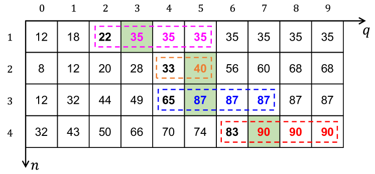
Figure 11: An example of computing $\{Q_{1}^{*},Q_{2}^{*},Q_{3}^{*},Q_{4}^{*}\}$ based on the table of $H(n,q)$ for all $1\leq n\leq 4$ and $0\leq q\leq 9$.

Appendix H

Similar as Section 6.1.3, we take the data mechanism $\kappa=1$ as an example to investigate how the MNO’s capacity cost $z$ affects the optimal contract items.

Fig. 12 shows the impact of the MNO’s capacity cost $z$. Specifically, there are a total of seven different contract items in the optimal contract. The seven curves in Fig. 12(a) represent the corresponding different data caps. We note that the optimal data caps (except the zero cap) decrease in the MNO’s capacity cost. Fig. 12(b) plots the corresponding subscription fees in the optimal contract. We find that

• The subscription fee of the zero-cap contract item (i.e., the bottom blue circle curve in Fig. 12(b)) does not change in the capacity cost $z$. This results from the individual rationality condition in (31a).

• The subscription fees of small-cap contract items (e.g., the cross and triangle curves in Fig. 12(b)) decrease in the MNO’s costs. While the subscription fees of the large-cap contract item (e.g., the diamond curves in Fig. 12(b)) increases in the MNO’s costs. Therefore, the large-cap contract item becomes less economical to the users (in terms of the average price $\Pi/Q$) as the MNO’s capacity cost increases. That is, the profit-maximizing MNO tends to compensate its capacity cost by charging those users who are willing to pay for the large-cap contract item.

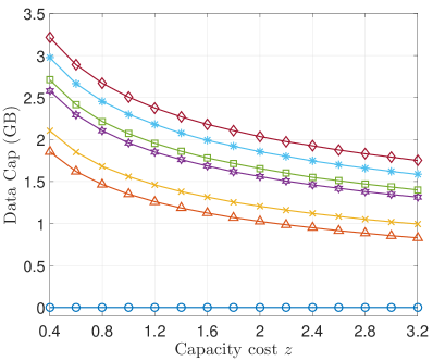
(a) Optimal data caps.

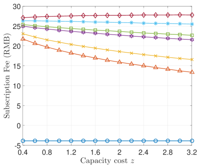
(b) Optimal subscription fees.

Figure 12: Impact of MNO’s capacity cost $z$.

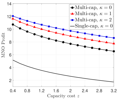
(a) MNO’s profit.

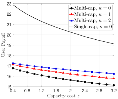
(b) All users’ payoff.

Figure 13: Impact of the MNO’s capacity cost $z$.

Next we evaluate the MNO’s profit and user’s payoffs in the four scenarios of Table IV under different capacity cost. In Fig. 13, the horizontal axises in the two sub-figures represent the MNO’s marginal capacity cost.

• Fig. 13(a) plots MNO’s profits in the four scenarios. Overall, the MNO’s profits decrease in its capacity cost $z$. By comparing single-cap traditional pricing benchmark and the multi-cap traditional pricing scheme, we note that the price discrimination under our optimal contract can significantly increase the MNO’s profit (176% on average). By comparing the three multi-cap curves, we find that the MNO obtains a higher profit under a more time-flexible data mechanism. Specifically, compared with Scenario (ii) (i.e., the circle curve), MNO’s profits increases by 12% on average in Scenario (iii) (i.e., the triangle curve) and 23% on average in Scenario (iv) (i.e., square curve). This implies that under the multi-cap scheme, offering a better time flexibility can further improve the MNO’s profit.

• Fig. 13(b) plots the users’ total expected payoff in four scenarios. First, we observe that users’ payoff decreases in the MNO’s capacity cost. By comparing the single-cap traditional pricing benchmark and the multi-cap traditional pricing scheme, we notice that the price discrimination under our optimal contract reduces users’ expected payoff (20% on average), which means that the MNO captures more consumer surplus through the price discrimination. Comparing the three multi-cap schemes, we find that the time-flexible data mechanisms can improve the users’ payoff. Specifically, compared with Scenario (ii) (i.e., the circle curve), users’ payoff increases by 3.1% on average in Scenario (iii) (i.e., the triangle curve) and 5.2% on average in Scenario (iv) (i.e., square curve).

Appendix I

In Section 6, we cluster the empirical data valuation and network substitutability into four groups, respectively. We then proceed the contract design based on the method in Section 5 for a total of sixteen user types. Next we investigate the impact of the number of clustered user types on the performance of the optimal contract.

TABLE V: Four cases of user type cluster.

Case	Data valuation	Network substitutability
$2\times 2$	$\{24.6,63.4\}$	$\{0.60,0.87\}$
$3\times 3$	$\{18.3,44.4,80.7\}$	$\{0.48,0.72,0.90\}$
$4\times 4$	$\{16.2,36.1,61.9,96.3\}$	$\{0.51,0.71,0.84,0.95\}$
$5\times 5$	$\{14.4,32.2,48.9,76.1,103.9\}$	$\{0.40,0.58,0.71,0.82,0.94\}$

(a) MNO’s profit.

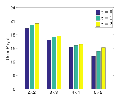
(b) All users’ expected payoff.

Figure 14: Impact of the number of clustered user types.

We will compare four scenarios, where the users’ each characteristic is clustered into two groups, three groups, four groups, and five groups, respectively. Table V shows the corresponding mean values of the users types in the four cases. Fig. 14 shows the performance of the optimal contract in the four cases under three data mechanisms. Here we let the operational cost be $c=6$RMB/GB and the capacity cost be $z=1.3$RMB/GB.

• Fig. 14(a) plots the MNO’s profits in the four cases under three different data mechanisms. Overall, the MNO’s profit increases in the number of clustered user types. Moreover, the time-flexible data mechanism can further increase the MNO’s profit given the number of user types.

• Fig. 14(b) plots all users’ average payoff in the four cases under three data mechanisms. Overall, all users’ average payoff decreases in the number of user types considered by the MNO. But a more time-flexible data mechanism increases the users’ payoff given the number of user types.

Based on the above discussion, we conclude that when the MNO divides the users into more types, the MNO’s profit increases but the users’ average payoff decreases. It means that a finer granularity price discrimination reduces the consumer surplus. In all cases, the time-flexible data mechanisms can increase both the MNO’s profit and users’ payoff, leading to a win-win situation.

References

- [1] Z. Wang, L. Gao, and J. Huang, “Multi-dimensional contract design for mobile data plan with time flexibility,” in 19th International Symposium on Mobile Ad Hoc Networking and Computing (MobiHoc), 2018.
- [2] ——, “A contract-theoretic design of mobile data plan with time flexibility,” in ACM Workshop on the Economics of Networks, Systems and Computation (NetEcon) (in conjunction with ACM EC), 2017.
- [3] S. Sen, C. Joe-Wong, S. Ha, and M. Chiang, “A survey of smart data pricing: Past proposals, current plans, and future trends,” ACM Computing Surveys (CSUR), vol. 46, no. 2, p. 15, 2013.
- [4] AT&T data plans. [Online]. Available: https://m.att.com/shopmobile/wireless/data-plans_12-7.html
- [5] J. Huang and L. Gao, “Wireless network pricing,” Synthesis Lectures on Communication Networks, vol. 6, no. 2, pp. 1–176, 2013.
- [6] AT&T Rollover Plan. [Online]. Available: https://www.att.com
- [7] China Mobile. [Online]. Available: http://www.10086.cn
- [8] Z. Wang, L. Gao, and J. Huang, “Exploring time flexibility in wireless data plans,” IEEE Transactions on Mobile Computing, 2018. [Online]. Available: https://arxiv.org/abs/1808.10569
- [9] Z. Wang, L. Gao, and J. Huang, “Duopoly Competition for Mobile Data Plans with Time Flexibility,” IEEE Transactions on Mobile Computing, 2019. [Online]. Available: https://arxiv.org/abs/1903.10878
- [10] X. Wang, R. T. Ma, and Y. Xu, “The role of data cap in optimal two-part network pricing,” IEEE/ACM Transactions on Networking, vol. 25, no. 6, pp. 3602–3615, 2017.
- [11] L. Zheng, C. Joe-Wong, M. Andrews, and M. Chiang, “Optimizing data plans: Usage dynamics in mobile data networks,” in IEEE International Conference on Computer Communications (INFOCOM), 2018.
- [12] Z. Xiong, S. Feng, D. Niyato, P. Wang, and Y. Zhang, “Economic analysis of network effects on sponsored content: a hierarchical game theoretic approach,” in IEEE Global Communications Conference (GLOBECOM), 2017.
- [13] X. Wang, L. Duan, and R. Zhang, “User-initiated data plan trading via a personal hotspot market,” IEEE Transactions on Wireless Communications, vol. 15, no. 11, pp. 7885–7898, 2016.
- [14] L. Zheng and C. Joe-Wong, “Understanding rollover data,” in IEEE INFOCOM Workshop on Smart Data Pricing, 2016.
- [15] Y. Wei, J. Yu, T. M. Lok, and L. Gao, “A novel mobile data contract design with time flexibility,” arXiv preprint arXiv:1806.07308, 2018.
- [16] Z. Wang, L. Gao, J. Huang, and B. Shou, “Economic viability of data trading with rollover,” in IEEE International Conference on Computer Communications (INFOCOM), 2019.
- [17] W. Dai and S. Jordan, “The effect of data caps upon isp service tier design and users,” ACM Transactions on Internet Technology (TOIT), vol. 15, no. 2, p. 8, 2015.
- [18] P. Bolton and M. Dewatripont, Contract theory. MIT press, 2005.
- [19] R. Deneckere and S. Severinov, “Multi-dimensional screening: a solution to a class of problems,” 2011.
- [20] R. P. McAfee and J. McMillan, “Multidimensional incentive compatibility and mechanism design,” Journal of Economic Theory, vol. 46, no. 2, pp. 335–354, 1988.
- [21] J.-C. Rochet and P. Choné, “Ironing, sweeping, and multidimensional screening,” Econometrica, pp. 783–826, 1998.
- [22] A. Lambrecht, K. Seim, and B. Skiera, “Does uncertainty matter? consumer behavior under three-part tariffs,” Marketing Science, vol. 26, no. 5, pp. 698–710, 2007.
- [23] A. Nevo, J. L. Turner, and J. W. Williams, “Usage-based pricing and demand for residential broadband,” Econometrica, vol. 84, no. 2, pp. 411–443, 2016.
- [24] R. T. Ma, “Usage-based pricing and competition in congestible network service markets,” IEEE/ACM Transactions on Networking, vol. 24, no. 5, pp. 3084–3097, 2016.
- [25] S. Sen, C. Joe-Wong, and S. Ha, “The economics of shared data plans,” in Annual Workshop on Information Technologies and Systems, 2012.
- [26] Q. Ma, L. Gao, Y.-F. Liu, and J. Huang, “Economic analysis of crowdsourced wireless community networks,” IEEE Transactions on Mobile Computing, no. 1, pp. 1–1, 2016.
- [27] Y. Kodratoff, Introduction to machine learning, 2014.
- [28] D. Fudenberg and J. Tirole, “Game theory,” 1991.
- [29] X. Wang, R. T. Ma, and Y. Xu, “On optimal two-sided pricing of congested networks,” Proceedings of the ACM on Measurement and Analysis of Computing Systems, vol. 1, no. 1, p. 7, 2017.
- [30] Y. Luo, L. Gao, and J. Huang, “An integrated spectrum and information market for green cognitive communications,” IEEE Journal on Selected Areas in Communications, vol. 34, no. 12, pp. 3326–3338, 2016.
- [31] L. Duan, J. Huang, and B. Shou, “Duopoly competition in dynamic spectrum leasing and pricing,” IEEE Transactions on Mobile Computing, vol. 11, no. 11, pp. 1706–1719, 2012.
- [32] S. Athey, “Single crossing properties and the existence of pure strategy equilibria in games of incomplete information,” Econometrica, vol. 69, no. 4, pp. 861–889, 2001.
- [33] L. Gao, X. Wang, Y. Xu, and Q. Zhang, “Spectrum trading in cognitive radio networks: A contract-theoretic modeling approach,” IEEE Journal on Selected Areas in Communications, vol. 29, no. 4, pp. 843–855, 2011.
- [34] L. Duan, L. Gao, and J. Huang, “Cooperative spectrum sharing: A contract-based approach,” IEEE Transactions on Mobile Computing, vol. 13, no. 1, 2014.
- [35] Y. Zhang, L. Song, W. Saad, Z. Dawy, and Z. Han, “Contract-based incentive mechanisms for device-to-device communications in cellular networks,” IEEE Journal on Selected Areas in Communications, vol. 33, no. 10, pp. 2144–2155, 2015.
- [36] Y. Zhang, L. Song, M. Pan, Z. Dawy, and Z. Han, “Non-cash auction for spectrum trading in cognitive radio networks: Contract theoretical model with joint adverse selection and moral hazard,” IEEE Journal on Selected Areas in Communications, vol. 35, no. 3, pp. 643–653, 2017.
- [37] R. Bellman, Dynamic programming. Courier Corporation, 2013.