A Neural Network-Evolutionary Computational Framework for Remaining Useful Life Estimation of Mechanical Systems

Abstract

This paper presents a framework for estimating the remaining useful life (RUL) of mechanical systems. The framework consists of a multi-layer perceptron and an evolutionary algorithm for optimizing the data-related parameters. The framework makes use of a strided time window to estimate the RUL for mechanical components. Tuning the data-related parameters can become a very time consuming task. The framework presented here automatically reshapes the data such that the efficiency of the model is increased. Furthermore, the complexity of the model is kept low, e.g. neural networks with few hidden layers and few neurons at each layer. Having simple models has several advantages like short training times and the capacity of being in environments with limited computational resources such as embedded systems. The proposed method is evaluated on the publicly available C-MAPSS dataset [1], its accuracy is compared against other state-of-the art methods for the same dataset.

1 Introduction

Traditionally, maintenance of mechanical systems has been carried out based on scheduling strategies. Such strategies are often costly and less capable of meeting the increasing demand of efficiency and reliability [2, 3]. Condition based maintenance (CBM) also known as intelligent prognostics and health management (PHM) allows for maintenance based on the current health of the system, thus cutting down the costs and increasing the reliability of the system [4]. Here, we refer to prognostics as the estimation of remaining useful life of a system. The remaining useful life (RUL) of the system can be estimated based on the historical data. This data-driven approach can help optimize maintenance schedules to avoid engineering failures and to save costs [5].

The existing PHM methods can be grouped into three different categories: model-based [6], data-driven [7, 8] and hybrid approaches [9, 10]. Model-based approaches attempt to incorporate physical models of the system into the estimation of the RUL. If the system degradation is modeled precisely, model-based approaches usually exhibit better performance than data-driven approaches [11]. This comes at the expense of having extensive a priori knowledge of the underlying system and having a fine-grained model of the system, which can involve expensive computations. On the other hand, data-driven approaches use pattern recognition to detect changes in system states. Data-driven approaches are appropriate when the understanding of the first principles of the system dynamics is not comprehensive or when the system is sufficiently complex such as jet engines, car engines and complex machineries, for which it is prohibitively difficult to develop an accurate model.

Common disadvantages for the data-driven approaches are that they usually exhibit wider confidence intervals than model-based approaches and that a fair amount of data is required for training. Many data-driven algorithms have been proposed. Good prognostics results have been achieved. Among the most popular algorithms we can find artificial neural networks (ANNs) [2], support vector machine (SVM) [12], Markov hidden chains (MHC) [13] and so on. Over the past few years, data-driven approaches have gained more attention in the PHM community. A number of machine learning techniques, especially neural networks, have been applied successfully to estimate the RUL of diverse mechanical systems. ANNs have demonstrated good performance in modeling highly nonlinear, complex, multi-dimensional systems without any prior knowledge on the system behavior [14]. While the confidence limits for the RUL predictions cannot be analytically provided [15], the neural network approaches are promising for prognostic problems.

Neural networks for estimating the RUL of jet engines have been previously explored in [16] where the authors propose a multi-layer perceptron (MLP) coupled with a feature extraction (FE) method and a time window for the generation of the features for the MLP. In the publication, the authors demonstrate that a moving window combined with a suitable feature extractor can improve the RUL prediction as compared with the studies with other similar methods in the literature. In [14], the authors explore a deep learning ANN architecture, the so-called convolutional neural networks (CNNs), where they demonstrate that by using a CNN without any pooling layers coupled with a time window, the predicted RUL is further improved.

In this paper we propose a novel framework for estimating the RUL of complex mechanical systems. The framework consists of a MLP to estimate the RUL of the system, coupled with an evolutionary algorithm for the fine tuning of data-related parameters. In this paper we refer to data-related parameters as parameters that define the shape, defined in terms of window size and window stride, and quality of the data, measured with respect to some performance indicators, used by the MLP. Please note that while this specific framework makes use of a MLP, the framework can in principle use several other learning algorithms, our main objective is the treatment of the data instead of the choice of a particular learning algorithm. The publicly available NASA C-MAPSS dataset [1] is used to assess the efficiency and reliability of the proposed framework, by efficiency we mean the complexity of the used regressor and reliability refers to the accuracy of the predictions made by the regressor. This approach allows for a simple and small MLP to obtain better results than those reported in the current literature while using less computing power.

The remainder of this paper is organized as follows. The C-MAPSS dataset is presented in Section 2. The framework and its components are thoroughly reviewed in Section 3. The method is evaluated using the C-MAPSS dataset in Section 4. A comparison with the state-of-the-art is also provided. Finally, the conclusions are presented in Section 5.

2 NASA C-MAPSS Dataset

The NASA C-MAPSS dataset is used to evaluate performance of the proposed method [1]. The C-MAPSS dataset contains simulated data produced using a model based simulation program developed by NASA. The dataset is further divided into 4 subsets composed of multi-variate temporal data obtained from 21 sensors.

For each of the 4 subsets, a training and a test set are provided. The training sets include run-to-failure sensor records of multiple aero-engines collected under different operational conditions and fault modes as described in Table 1.

	C-MAPSS
Dataset	FD001	FD002	FD003	FD004
Training Trajectories	100	260	100	248
Test Trajectories	100	259	100	248
Operating Conditions	1	6	1	6
Fault Modes	1	1	2	2

Table 1: C-MAPSS dataset details.

The data is arranged in an $N\times 26$ matrix where $N$ is the number of data points in each subset. The first two variables represent the engine and cycle numbers, respectively. The following three variables are operational settings which correspond to the conditions in Table 1 and have a substantial effect on the engine performance. The remaining variables represent the 21 sensor readings that contain the information about the engine degradation over time.

Each trajectory within the training and test sets represents the life cycles of the engine. Each engine is simulated with different initial health conditions, i.e. no initial faults. For each trajectory of an engine the last data entry corresponds to the cycle at which the engine is found faulty. On the other hand, the trajectories of the test sets terminate at some point prior to failure, hence the need to predict the remaining useful life. The aim of the MLP model is to predict the RUL of each engine in the test set. The actual RUL values of test trajectories are also included in the dataset for verification. Further discussions of the dataset and details on how the data is generated can be found in [17].

2.1 Performance Metrics

To evaluate the performance of the proposed approach on the C-MAPSS dataset, we make use of two scoring indicators, namely the Root Mean Squared Error (RMSE) denoted as $E_{\scriptscriptstyle RMS}(\mathbf{e})$ and a score proposed in [17] which we refer as the RUL Health Score (RHS) denoted as $E_{\scriptscriptstyle RH}(\mathbf{e})$. The two scores are defined as follows,

$$E_{\scriptscriptstyle RMS}=\sqrt{\frac{1}{n}\sum_{i=1}^{N}{e_{i}^{2}}}$$ (1)

$$E_{\scriptscriptstyle RH} =\frac{1}{n}\sum_{i=1}^{N}{s_{i}}$$

$$s_{i} =\begin{cases}\exp(-\frac{e_{i}}{13})-1,&e_{i}<0\\ \exp(\frac{e_{i}}{10})-1,&e_{i}\geq 0,\end{cases}$$ (2)

where $n$ is the total number of samples in the test set and $\mathbf{e}=\mathbf{\hat{y}}-\mathbf{y}$ is the error between the estimated RUL values $\mathbf{\hat{y}}$, and the actual RUL values $\mathbf{y}$ for each engine within the test set. It is important to note that $E_{\scriptscriptstyle RH}(\mathbf{e})$ penalizes late predictions more than early predictions since usually late predictions lead to more severe consequences in fields such as aerospace.

3 Framework Description

n this section, the proposed ANN-EA based method for prognostics is presented. The method makes use of a multi-layer perceptron (MLP) as the main regressor for estimating the RUL of the engines in the C-MAPSS dataset. The choice of a MLP as the learning algorithm instead of any of the other choices (SVM, RNN, CNN, Least-Squares, etc) obeys to the fact that MLPs are in general good for nonlinear data like the one exhibited by the C-MAPSS dataset, but at the same time are less computationally expensive than some of the more sophisticated algorithms as the CNN or the RNN. Indeed, the RNN may be a more suitable choice for this particular problem since it involves time-sequenced data, nevertheless, we will show that by doing a fine tuning of the data-related parameters (and thus data processing), the inference power of a simple MLP can be competitive even when compared against that of an RNN. For the training sets, the feature vectors are generated by using a moving time window while a label vector is generated with the RUL of the engine. The label has a constant RUL for the early cycles of the simulation, and becomes a linearly decreasing function of the cycle in the remaining cycles. This is the so-called piece-wise linear degradation model [18]. For the test set, a time window is taken from the last sensor readings of the engine. The data of the test set is used to predict the RUL of the engine.

The window-size $n_{w}$, window-stride $n_{s}$, and early-RUL $R_{e}$ are data-related parameters, which for the sake of clarity and formalism in this study, form a vector $\mathbf{v}\in\mathbb{Z}^{3}$ such that $\mathbf{v}=(n_{w},n_{s},R_{e})$. The vector $\mathbf{v}$ has a considerable impact on the quality of the predictions by the regressor. It is computationally intensive to find the best parameters of $\mathbf{v}$ given the search space inherent to these parameters. We propose an evolutionary algorithm to optimize the data-related parameters $\mathbf{v}$. The optimized parameter set $\mathbf{v}$ allows the use of a simple neural network architecture while attaining better results in terms of the quality of the predictions compared with the results by other methods in the literature.

3.1 The Network Architecture

After careful examinations of the C-MAPSS dataset, we propose to use a rather simple MLP architecture for all the four subsets of the data. The choice of a simple architecture over a more complex one follows the fact that simpler neural networks are less computationally expensive to train, furthermore, the inference is done also faster since less operations are involved. To measure the simplicity/complexity of a neural network we use the number of trainable parameters (weights) of the neural network, usually the more trainable parameters in a network the more computations that need be done, thus increasing the computational burden of the training/inference process. The implementations are done in Python using the Keras/Tensorflow environment. The source code is publicly available at the git repository https://github.com/dlaredo/NASA_RUL_-CMAPS- [19].

The choice of the network architecture is made by following an iterative process, our goal was to find a good compromise between efficiency (simple neural network models) and reliability (scores obtained by the model using the RMSE metric): We compared 6 different architectures (see Appendix A), training each for $100$ epochs using a mini-batch size of $512$ and averaging their results on a cross-validation set for $10$ different runs. L1 (Lasso) and L2 regularization (Ridge) [20] are used to prevent over-fitting. L1 regularization penalizes the sum of the absolute value of the weights and biases of the networks, while L2 regularization penalizes the sum of the squared value of the weights and biases. The data-related parameters $\mathbf{v}$ used for this experiment are $\mathbf{v}=(30,1,140)$. Two objectives are pursued during the iterations: the architecture must be minimal in terms of the number of trainable parameters and the performance indicators must be minimized. Table 2 summarizes the results for each tested architecture.

	RMSE				RHS
Tested Architecture	Min.	Max.	Avg.	STD	Min.	Max.	Avg.	STD
Architecture 1	15.51	17.15	16.22	0.49	4.60	7.66	5.98	0.91
Architecture 2	15.24	16.46	15.87	0.47	4.07	6.26	5.29	0.82
Architecture 3	15.77	17.27	16.15	0.45	5.11	8.25	5.93	0.94
Architecture 4	15.13	17.01	15.97	0.47	3.90	7.54	5.65	1.2
Architecture 5	16.39	17.14	16.81	0.23	5.19	6.58	5.98	0.42
Architecture 6	16.42	17.36	16.87	0.30	5.15	7.09	6.12	0.62

Table 2: Results for different architectures for subset 1, 100 epochs.

Table 3 presents the architecture chosen for the remainder of this work (which provides the best compromise between compactness and performance among the tested architectures). Each row in the table represents a neural network layer while each column describes each one of the key parameters of the layer such as the type of layer, number of neurons in the layer, activation function of the layer and whether regularization is used, where L1 denotes the L1 regularization factor and L2 denotes the L2 regularization factor, the order in which the layers are appended from the table is top-bottom. From here on we refer to this neural network model as $\phi(.)$.

Layer	Neurons	Activation	Additional Information
Fully connected	20	ReLU	$L1=0.1,L2=0.2$
Fully connected	20	ReLU	$L1=0.1,L2=0.2$
Fully connected	1	Linear	$L1=0.1,L2=0.2$

Table 3: Proposed neural network architecture $\phi(.)$.

3.2 Shaping the Data

This section covers the data pre-processing applied to the raw sensor readings in each of the datasets. Although the original datasets contain $21$ different sensor readings, some of the sensors do not present much variance or convey redundant information, our choice of the sensors is based on previous studies such as [16, 14] where it was discovered that some sensor values do not vary at all throughout the entire engine life cycle while some others are redundant according to PCA or clustering analysis. These sensors are therefore discarded. In the end, only $14$ sensor readings out of the $21$ are considered for this study. Their indices are $\left\{2,3,4,7,8,9,11,12,13,14,15,17,20,21\right\}$. The raw measurements are then used to create the strided time windows with window-size $n_{w}$ and window-stride $n_{s}$. For the training labels, $R_{e}$ is used at the early stages and then the RUL is linearly decreased. Assuming $\mathbf{x}\in\mathbb{R}^{m}$ is the vector whose components are the sensor readings at each time stamp, then the min-max normalized vector $\mathbf{\hat{x}}$ can be computed by means of the following formula:

$$\hat{x}_{i}=2*\frac{x_{i}-min(x_{i})}{max(x_{i})-min(x_{i})}-1.$$ (3)

3.2.1 Time Window and Stride

In multivariate time-series problems such as RUL, more information can be generally obtained from the temporal sequence of the data as compared with the multivariate data point at a single time stamp. For a time window of size $n_{w}$ with a stride $n_{s}=1$, all the sensor readings in the time window form a feature vector $\mathbf{x}\in\mathbb{R}^{s*n_{w}}$, where $s$ denotes the number of sensors being read. Stacking together $m_{w}$ of this time windows forms feature vector $\mathbf{X}\in\mathbb{R}^{m_{w}\times s*n_{w}}$ while its corresponding RUL values are defined as $\mathbf{y}\in\mathbb{Z}^{m}$. It is important to mention that the shape of $\mathbf{X}$ defines the number of input neurons for the neural network, therefore changing the shape of $\mathbf{X}$ effectively changes the number of inputs to the neural network. This approach has successfully been tested in [14, 16] where the authors propose the use of a moving window with sizes ranging from 20 to 30. We propose not only the use of a moving time window, but also a strided time window that updates more than one element ($n_{s}>1$) at the time. A graphical depiction of the strided time window is shown in Figure 1. For Figure 1 the numbers and time-stamps are just illustrative, the window size exemplified is of 30 time-stamps while the stride is of 3 time-stamps.

Figure 1: Graphical depiction of the time window used in this framework.

Figure 2 shows an example of how to form a sample vector, in this example $s=14$, $n_{w}=5$ and $n_{s}=4$. Each one of the plotted lines denotes the readings for each of the fourteen chosen sensors. The dashed vertical lines (black lines) represent the size of the window, in this case we depict a window size of $5$ cycles. For the next window (red dashed lines) the time window is advanced by a stride of $4$ cycles, note that some sensor readings may be overlapped for different moving windows. For every window, the sensor readings are appended one after another to form a vector of $14*5$ features, for this specific case the unrolled vector will be of $70$ features.

Figure 2: Window size and stride example.

The use of a strided time window allows for the regressor to take advantage not only of the previous information, but also to control the ratio at which the algorithm is fed with new information. With the usual time window approach, only one point is updated for every new time window. The strided time window considered in this study allows for updating more than one point at the time for the algorithm to make use of the new information with less iterations. Our choice of the strided time window is inspired by the use of strided convolutions in Convolutional Neural Networks [21]. Further studies of the impact of the stride on the prediction should be done in the future.

3.2.2 Piecewise Linear Degradation Model

Different from common regression problems, the desired output value of the input data is difficult to determine for a RUL problem. It is usually impossible to evaluate the precise health condition and estimate the RUL of the system at each time step without an accurate physics based model. For this popular dataset, a piece-wise linear degradation model has been proposed in [18]. The model assumes that the engines have a constant RUL label in the early cycles, and then the RUL starts degrading linearly until it reaches 0 as shown in Figure 3. The piece-wise linear degradation assumption is used in this work. We denote the value of the RUL in the early cycles as $R_{e}$. Initially, $R_{e}$ is randomly chosen between 90 and 140 cycles which is a reasonable range of values for this particular application. When the difference between the cycle count in the time window and the terminating cycle of the training data is less than the initial value of $R_{e}$, $R_{e}$ begins the linear descent toward the terminating cycle.

Figure 3: Piece-wise linear degradation for RUL.

3.3 Optimal Data Parameters

As mentioned in the previous sections the choice of the data-related parameters $\mathbf{v}$ has a large impact on the performance of the regressor. In this section, we present a method for picking the optimal combination of the data-related parameters $n_{w}$, $n_{s}$ and $R_{e}$ while being computationally efficient.

Vector $\mathbf{v}=(n_{w},n_{s},R_{e})$ components specific to the C-MAPSS dataset are bounded such that $n_{w}\in\left[1,b\right]$, $n_{s}\in\left[1,10\right]$, and $R_{e}\in\left[90,140\right]$, where all the variables are integer. The value of $b$ is different for different subsets of the data, Table 4 shows the different values of $b$ for each subset.

	FD001	FD002	FD003	FD004
$b$	30	20	30	18

Table 4: Allowed values for $b$ per subset.

Let $\mathbf{X}(\mathbf{v})$ be the training/cross-validate/test sets parametrized by $\mathbf{v}$ and $\mathbf{\hat{y}}(\mathbf{v})=\phi(\mathbf{X}(\mathbf{v});\boldsymbol{\theta})$ be the predicted RUL values of our model $\phi(.)$ with $\mathbf{X}(\mathbf{v})$. Thus, $E_{\scriptscriptstyle RMS}$ depends directly on the choice of $\mathbf{v}$ since $\phi(.)$ is fixed (See Section 2.1). Here we propose to solve the following optimization problem

$$\underset{\mathbf{v}\in\mathbb{Z}^{3}}{\mathrm{min}\;\;}E_{\scriptscriptstyle RMS}(\mathbf{v}).$$ (4)

The problem to find optimal data-related parameters has no analytic descriptions. Therefore, no gradient information is available. An evolutionary algorithm is the natural choice for this optimization problem. Nevertheless, since the computation of the error $E_{\scriptscriptstyle RMS}(\mathbf{v})$ requires re-training $\phi(.)$ an strategy to make the optimization process computationally efficient must be devised.

3.3.1 True Optimal Data Parameters

The finite size of C-MAPSS dataset and finite search space of $\mathbf{v}$ allow an exhaustive search to be performed in order to find the true optimal data-related parameters. We would like to emphasize that although exhaustive search is possible for the C-MAPSS dataset, it is in no way a possibility in a more general setting. Nevertheless, the possibility to perform exhaustive search on the C-MAPSS dataset can be exploited to demonstrate the accuracy of the chosen EA and of the framework overall. In the following studies, we use the results and computational efforts of the exhaustive search as benchmarks to examine the accuracy and efficiency of the proposed approach.

We should note that the subsets of the data FD001 and FD003 have similar features and that the subsets FD002 and FD004 have similar features. Because of this, we have decided to just optimize the data-related parameters by considering the subsets FD001 and FD002 only. An exhaustive search is performed to find the true optimal values for $\mathbf{v}$. The MLP is only trained for $20$ epochs. Table 5 shows the optimal as well as the worst combinations of data-related parameters and the total number of function evaluations used by the exhaustive search. It is important to notice that for this experiment the window size is limited to be larger than or equal to $15$.

Dataset	argmin $\mathbf{v}$	min $E_{\scriptscriptstyle RMS}(\mathbf{v})$	argmax $\mathbf{v}$	max $E_{\scriptscriptstyle RMS}(\mathbf{v})$	Function evals.
FD001	$\left[24,1,127\right]$	$15.11$	$\left[25,10,94\right]$	$85.19$	8160
FD002	$\left[16,1,138\right]$	$30.93$	$\left[17,10,99\right]$	$59.78$	3060

Table 5: Exhaustive search results for subsets FD001 and F002.

Numerical experiments seem to suggest that, at least for CMAPSS dataset, the window size plays a big role in terms of the meaningful information used for prediction by the MLP. It also reflects the history-dependent nature of the aircraft engine degradation process. Furthermore, overlapping in the generated time windows seems to benefit the generated sequences of sensors.

3.3.2 Evolutionary Algorithm for Optimal Data Parameters

Evolutionary algorithms (EAs) are a family of methods for optimization problems. The methods do not make any assumptions about the problem, treating it as a black box that merely provides a measure of quality given a candidate solution. Furthermore, EAs do not require the gradient when searching for optimal solutions, making them very suitable for applications such as neural networks.

For the current application, the differential evolution (DE) method is chosen as the optimization algorithm [22]. Though other meta-heuristic algorithms may also be suitable for this application, the DE has established as one of the most reliable, robust and easy to use EAs. Furthermore, a ready to use Python implementation is available through the scipy package [23]. Although the DE method does not have special operators for treating integer variables, a very simple modification to the algorithm, i.e. rounding every component of a candidate solution to its nearest integer, is used for this work.

As mentioned earlier, evolutionary algorithms such as the DE use several function evaluations when searching for the optimal solutions. It is important to consider that, for this application, one function evaluation requires retraining the neural network from scratch. This is not a desirable scenario, as obtaining the optimal data-related parameters would entail an extensive computational effort. Instead of running the DE for several iterations and with a large population size, we propose to run it just for $30$ iterations, i.e. the generations in the literature of evolutionary computation, with a population size of $12$, which seems reasonable given the size of the search space of $\mathbf{v}$.

During the optimization, the MLP is trained for only $20$ epochs. The small number of epochs of training the MLP is reasonable in this case because a small batch of data is used in the training, because we only look for the trend of the scoring indicators. Furthermore, it is common to observe that the parameters leading to lower score values in the early stages of the training are more likely to provide better performance after more epochs of training. The settings of the DE algorithm to find the optimal data-related parameters are listed in Table 6.

Population Size	Generations	Strategy	MLP epochs
12	30	Best1Bin [24]	20

Table 6: Differential evolution hyper-parameters.

The optimal data-related parameters for the subsets FD001 and FD002 found by the DE algorithm are listed in Table 7. As can be observed, the results are in fact very close to the true optimal ones in Table 5 for both the subsets of the data. The computational effort is reduced by one order of magnitude when using the DE method as compared to the exhaustive search for the true optimal parameters. From the results in Table 7, it can be observed that the maximum allowable time window is always preferred while, on the other hand, small window strides yield better results. For the case of early RUL, it can be observed that larger values of $R_{e}$ are favored.

Dataset	argmin $\mathbf{v}$	min $E_{\scriptscriptstyle RMS}(\mathbf{v})$	Function evals.
FD001	$\left[24,1,129\right]$	$15.24$	372
FD002	$\left[17,1,139\right]$	$30.95$	372

Table 7: Data-related parameters for each subset obtained with differential evolution.

3.4 The Estimation Algorithm

Having described the major building blocks of the proposed method, we now introduce the complete framework in the form of Algorithm 1.

Data: Training/testing data $\mathbf{X}\in\mathbb{R}^{m_{w}\times s*n_{w}}$

Input : Initial set of data-related parameters $\mathbf{v}\in\mathbb{Z}^{3}$, , training labels $\mathbf{y}\in\mathbb{Z}^{m}$ and number of training epochs for each evaluation of $\phi(\mathbf{v})$.

Output : Optimal set of data-related parameters $\mathbf{v}^{*}\in\mathbb{Z}^{3}$.

Choose regressor architecture (ANN, SVM, linear/logistic regression, etc).

Define $\phi(\mathbf{v})$ as in Section 3.3.

Optimize $\phi(\mathbf{v})$, by means of an evolutionary algorithm, using the proposed guidelines from Section 3.3.2.

Use $\mathbf{v}^{*}$ to train the regressor for as many epochs as needed.

Algorithm 1 ANN-EA RUL estimation framework.

4 Evaluation of the Proposed Method

4.1 Experimental settings

In this section, we evaluate the performance of the proposed method. The architecture of the MLP is described in Table 3. We define an experiment as the process of training the MLP on any of the subsets (FD001 to FD004) and evaluate its performance using the subset’s test set. The combinations of the optimal window size $n_{w}$, window stride $n_{s}$ and early RUL $R_{e}$ are presented in Table 8. We perform $10$ different experiments for each data subset, the MLP is trained for 200 epochs using the train set for the corresponding data subset and evaluated using the subset’s test set. The results for each dataset subset are averaged and presented in Table 9. Furthermore, the best model is saved and later used to generate the results presented in Section 4.2. All of the experiments were run using the Keras/Tensorflow framework, an NVIDIA GeForce 1080Ti GPU was used to speed up the training process.

Dataset	$n_{w}$	$n_{s}$	$R_{e}$	Input size (neurons)
FD001	24	1	129	336
FD002	17	1	139	238
FD003	24	1	129	336
FD004	17	1	139	238

Table 8: Data-related parameters for each subset as obtained by DE.

4.2 Experimental results

The obtained results for $\phi(\mathbf{v})$ using the above setting are presented in Table 9. Notice that the performances obtained for datasets FD001 and FD002 are improved as compared with the results in Table 7. This is due to the fact that the MLP is trained for more epochs, thus obtaining better results.

	$E_{\scriptscriptstyle RMS}$				$E_{\scriptscriptstyle RH}$
Data Subset	min	max	avg	STD	min	max	avg	STD
FD001	14.24	14.57	14.39	0.11	3.25	3.58	3.37	0.11
FD002	28.90	29.23	29.09	0.11	45.99	53.90	50.69	2.17
FD003	14.74	16.18	15.42	0.50	4.36	6.85	5.33	0.95
FD004	33.25	35.10	34.74	0.53	58.52	78.62	74.77	5.88

Table 9: Scores for each dataset using the data-related parameters obtained by DE.

We now compare the predicted RUL values versus the real RUL values for each of the datasets. For Figures 4 to 7 we plot on the top sub-figure the predicted RUL values (red lines) vs the real RUL values (green lines) while on the bottom sub-figure we plot the error between real RUL and predicted RUL.

Figure 4 shows the comparison for subset FD001, it can be observed that the predicted RUL values closely follow the real RUL values with the exception of a pair of engines. The error remains small for most of the engines. Meanwhile, for FD002 it can be observed in Figure 5 that the regressor overshoots several of the RUL predictions, especially in the positive spectrum. That is, the method predicts a RUL when in reality the real RUL is less than the predicted value. This is more evident in the second subplot where the maximum error is $138$ at the magenta peak in the leftmost part of the plot.

Figure 6 shows that for FD003 the predictions follow closely the real RUL values. The behavior for FD004 is similar to FD002 as depicted in Figure 7, with most of the error such that the predictions of the RUL are larger than the real value.

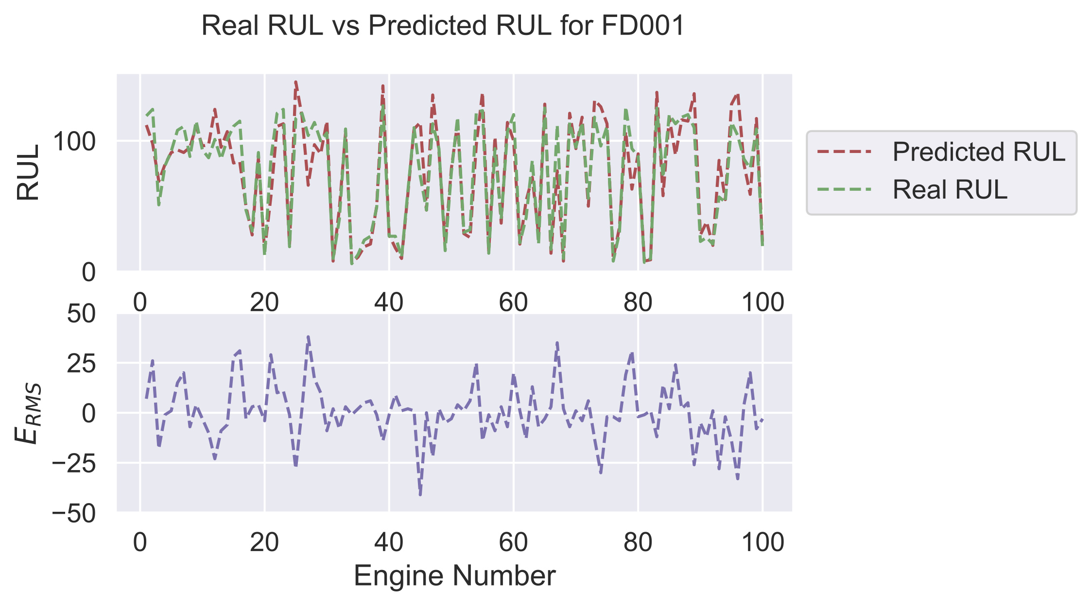
Figure 4: Comparison of predicted RUL values vs real RUL values for dataset FD001

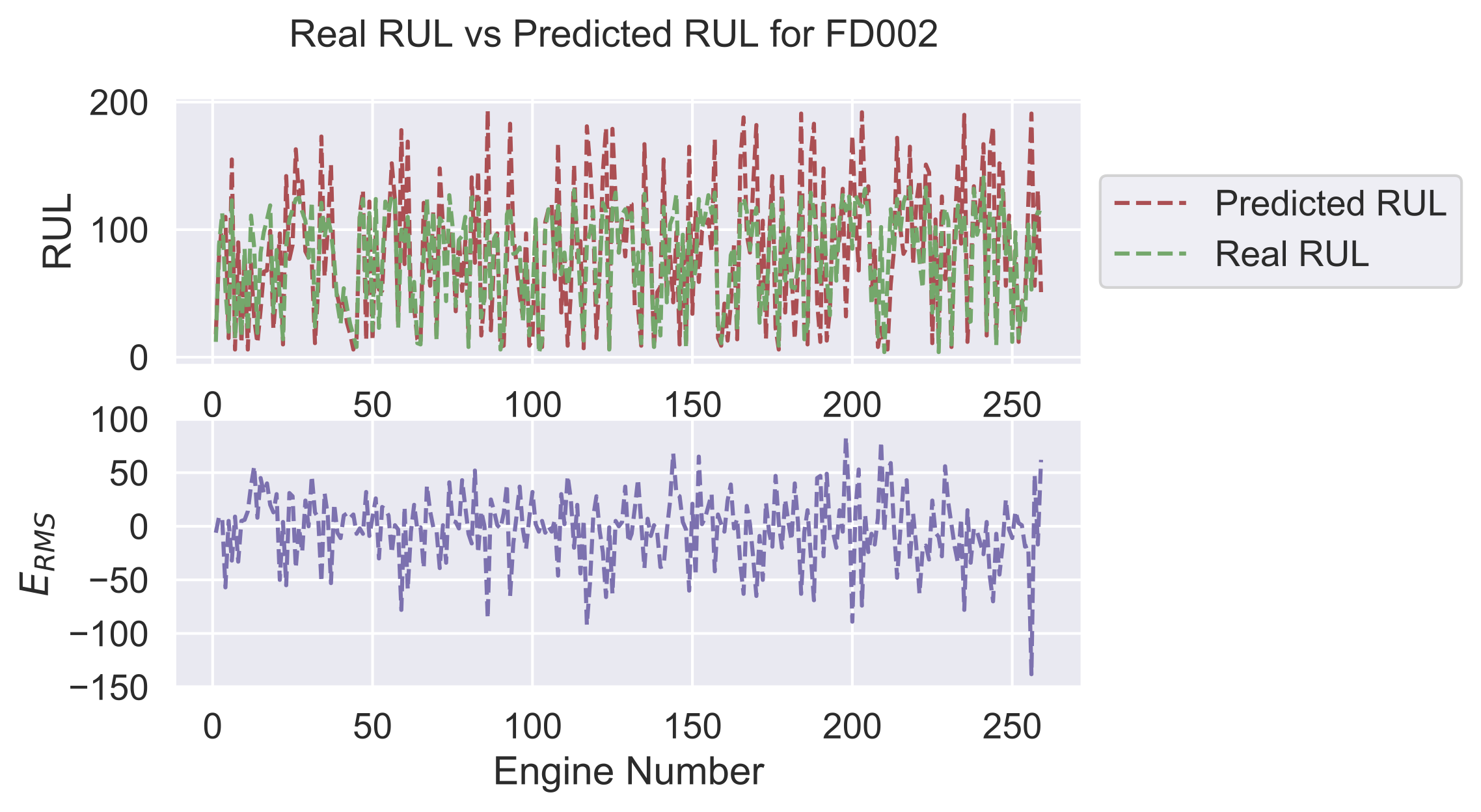
Figure 5: Comparison of predicted RUL values vs real RUL values for dataset FD002

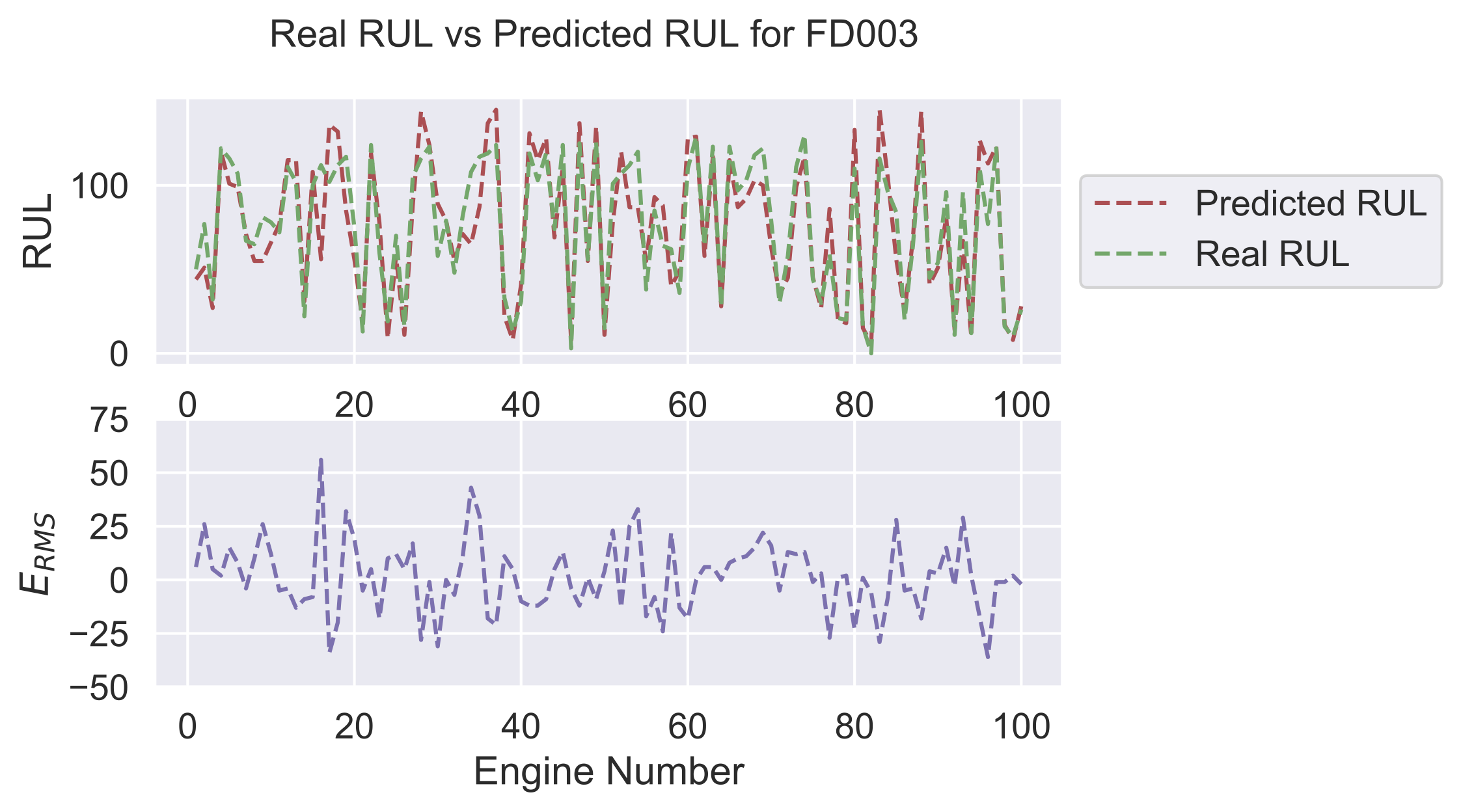
Figure 6: Comparison of predicted RUL values vs real RUL values for dataset FD003

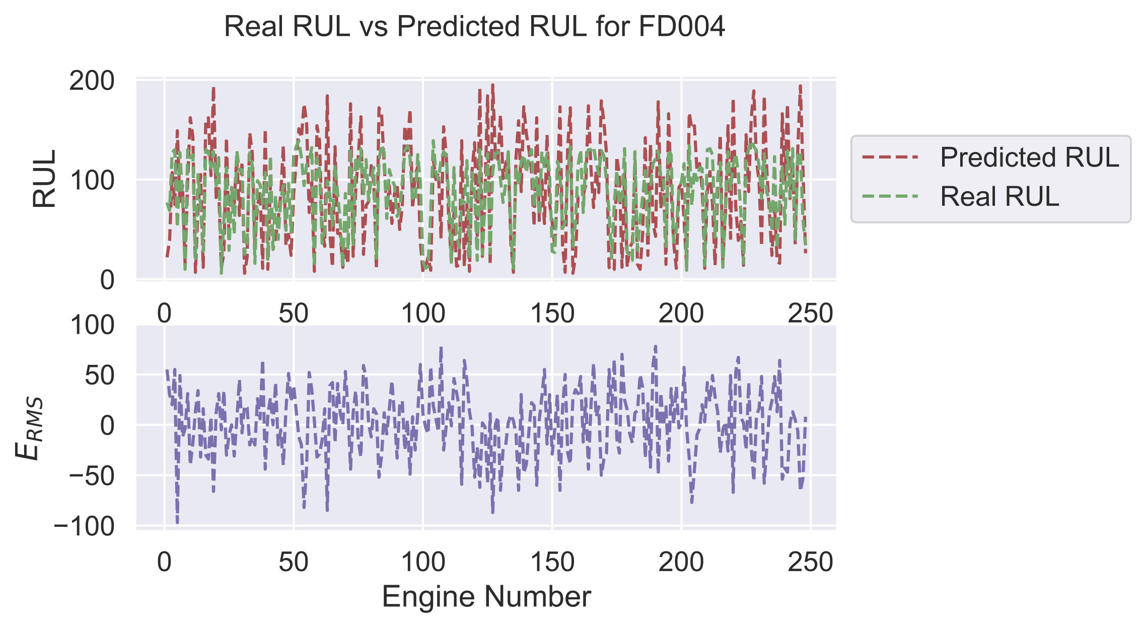
Figure 7: Comparison of predicted RUL values vs real RUL values for dataset FD004

Finally, Figure 8 shows that most of the RUL predictions by the method are highly accurate. In the case of FD001, the predictions of $50\%$ of the engines is smaller than $6$ cycles. In the case of FD002, the predictions are acceptable with the error of first quartile being lower than $6$ cycles and the error for $50\%$ of the engines being less than $19$ cycles. The cases for FD003 and FD004 are similar to FD001 and FD002, respectively.

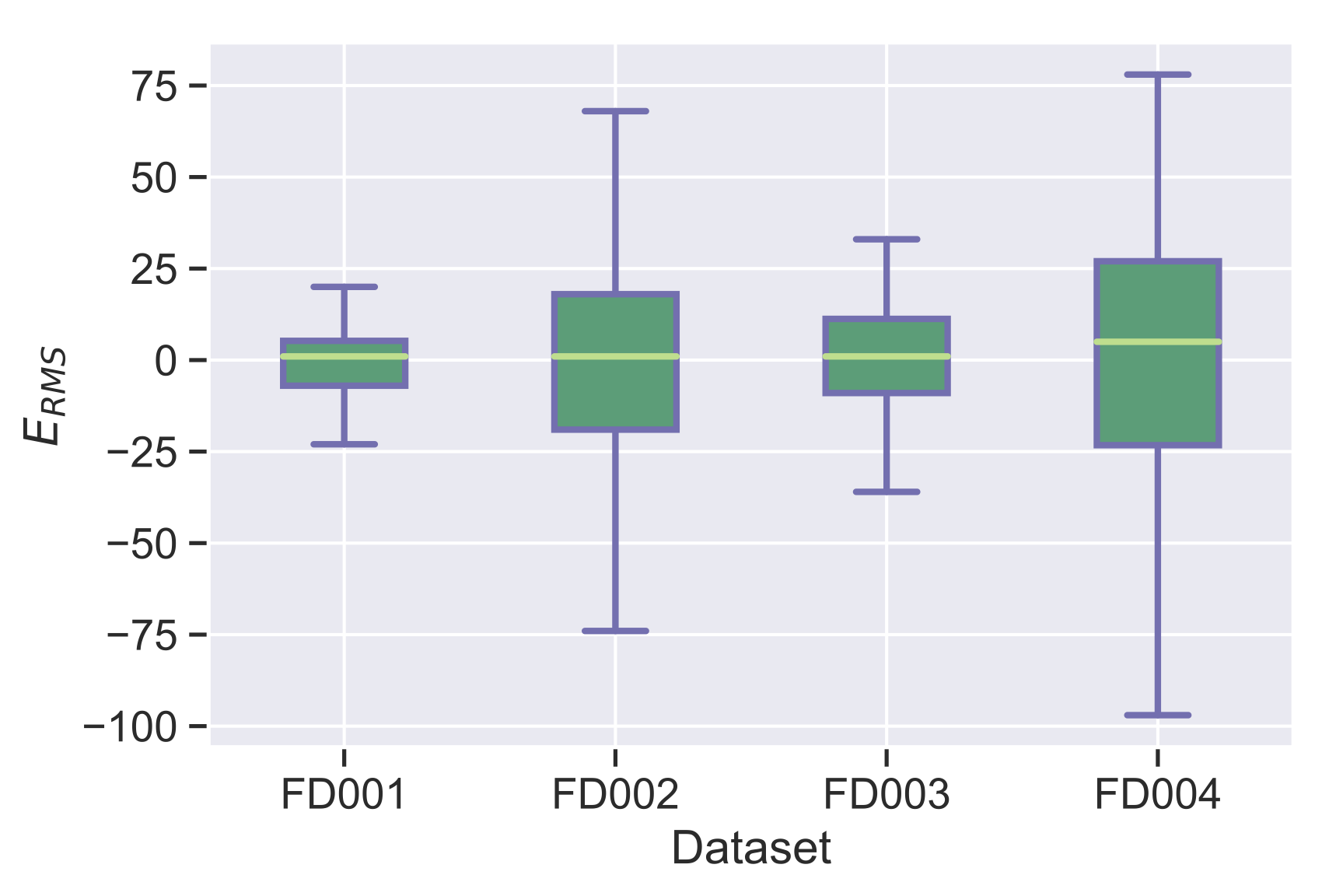
Figure 8: Prediction error of the MLP for each dataset.

Two conclusions can be drawn from the previous discussions. First, it can be observed that the number of operating conditions has a larger impact on the complexity of the data than the number of fault modes. This is because the subsets FD002 and FD004 exhibit larger errors than the subsets FD001 and FD003, although the general trend of prediction errors is similar among those two groups of data sets. Second, for the subsets FD002 and FD004, most of the error is related to the predictions larger than the real RUL values. Another observation is that larger window sizes usually lead to better predictions. This may be related to the history-dependent nature of the physical problem.

4.3 Comparison with other approaches

The performance of the proposed method is also compared against other state-of-the-art methods. The methods chosen for the comparison obey to two criteria: 1) that the method used is a machine learning (or statistical) method and 2) that the method is recent (6 years old at most). Most of the methods chosen here have only reported results on the test set FD001 in terms of $E_{rms}$. The results are shown in Table 10. The $E_{rms}$ value of the proposed method in Table 10 is the mean value of 10 independent runs. The values of other methods are identical to those reported in their respective original papers.

Method	$E_{rms}$
ESN trained by Kalman Filter [25]	63.45
Support Vector Machine Classifier [26]	29.82
Time Window Neural Network [16]	15.16
Multi-objective deep belief networks ensemble [27]	15.04
Deep Convolutional Neural Network [28]	18.45
Proposed method with $n_{w}=30$, $n_{s}=1$ and $R_{e}=128$	14.39
Modified approach with classified sub-models of the ESN [25].	7.021
Only 80 of 100 engines predicted
Deep CNN with time window [14].	13.32
RNN-Encoder-Decoder [29].	12.93

Table 10: Performance comparison of the proposed method and the latest related papers on the C-MAPSS dataset.

From the comparison studies, we can conclude that the proposed method performs better than the majority of the chosen methods when taking into consideration the whole dataset FD001. Two existing methods come close to the performance of the proposed approach here, namely the time window ANN [16] and the Networks Ensemble [27]. While the performance of these two methods comes close to the results of the proposed method, our method is computationally more efficient. We believe that the use of the time window with a proper size makes the difference. Notice that three of the methods presented in Table 10 perform better than the proposed method, namely, the Convolutional Neural Network [14], the RNN-Encoder-Decoder [29] and the modified ESN [25]. Nevertheless in the case of [25], the method can only predict 80 out of the 100 total engines while the deep CNN [14] and RNN [29] approaches are much more computationally expensive than the MLP used in this work. In the case of the method proposed in [14], the neural network model has four layers of convolutions and two more layers of fully connected layers. On the other hand, the RNN-Encoder-Decoder [29] makes use of a much more complicated scheme of two RNNs, one for encoding the sequences and one for decoding them. While specialized libraries such as TensorFlow or Keras make RNNs easier to use, they still remain up to date as some of the most computationally expensive architecture to train given their sequential nature. Finally, we would like to emphasize that the used MLP for this approach is one of the simplest ones in the reviewed literature. Furthermore, the framework proposed is simple to understand and implement, robust, generic and light-weight. These are the features important to highlight when comparing the proposed method against other state-of-the-art approaches.

5 Conclusions

We have presented a novel framework for predicting the RUL of mechanical components. While the method has been tested on the jet-engine dataset C-MAPSS, the method is general enough such that it can be applied to other similar systems. The framework makes use of a strided moving time window to generate the training and test records. A shallow MLP to make the predictions of the RUL has been found to be sufficient for the C-MAPSS dataset. The evolutionary algorithm DE needs to be run just once to find the best data-related parameters that optimize the scoring functions. The resulting model of the application of the framework presented in this paper demonstrated to be accurate and computationally efficient, specially when applied to large datasets in real applications. The compactness of the resulting model makes it suitable for applications that have limited computational resources such as embedded systems. It is important to note that the framework itself does involve some computations, nevertheless such computations are done off-line. Furthermore, the comparison with other state-of-the-art methods has shown that the proposed method is the best overall performer.

Two major features of the proposed framework are its generality and scalability. While for this study, specific regressors and evolutionary algorithms are chosen, many other combinations are possible and may be more suitable for different applications. Furthermore, the framework can, in principle, be used for model-construction, i.e. generating the best possible neural network architecture tailored to a specific application. Thus, future work will consider extensions to the framework to make it applicable to tasks such as model selection. An analysis of the influence of the window stride parameter $n_{s}$ will also be considered for future work.

References

Appendix A Tested Neural Network Architectures

In this appendix we present the tested neural network architectures. Each table represents a neural network model. Each row in the table represents a neural network layer while each column describes each one of the key parameters of the layer such as the type of layer, number of neurons in the layer, activation function of the layer and whether regularization is used, where L1 denotes the L1 regularization factor and L2 denotes the L2 regularization factor, the order in which the layers are appended from the table is top-bottom.

Table 1: Proposed neural network architecture 1.

Layer	Neurons	Activation	Additional Information
Fully connected	20	ReLU	L1 = 0.1, L2 = 0.2
Fully connected	20	ReLU	L1 = 0.1, L2 = 0.2
Fully connected	1	Linear	L1 = 0.1, L2 = 0.2

Table 2: Proposed neural network architecture 2.

Layer	Neurons	Activation	Additional Information
Fully connected	50	ReLU	L1 = 0.1, L2 = 0.2
Fully connected	20	ReLU	L1 = 0.1, L2 = 0.2
Fully connected	1	Linear	L1 = 0.1, L2 = 0.2

Table 3: Proposed neural network architecture 3.

Layer	Neurons	Activation	Additional Information
Fully connected	100	ReLU	L1 = 0.1, L2 = 0.2
Fully connected	50	ReLU	L1 = 0.1, L2 = 0.2
Fully connected	1	Linear	L1 = 0.1, L2 = 0.2

Table 4: Proposed neural network architecture 4.

Layer	Neurons	Activation	Additional Information
Fully connected	250	ReLU	L1 = 0.1, L2 = 0.2
Fully connected	50	ReLU	L1 = 0.1, L2 = 0.2
Fully connected	1	Linear	L1 = 0.1, L2 = 0.2

Table 5: Proposed neural network architecture 5.

Layer	Neurons	Activation	Additional Information
Fully connected	20	ReLU	L1 = 0.1, L2 = 0.2
Fully connected	1	Linear	L1 = 0.1, L2 = 0.2

Table 6: Proposed neural network architecture 6.

Layer	Neurons	Activation	Additional Information
Fully connected	10	ReLU	L1 = 0.1, L2 = 0.2
Fully connected	1	Linear	L1 = 0.1, L2 = 0.2

Appendix B Activation functions definitions

Here we define some of the activation functions used in our neural network models. For the following definitions assume a vector $\mathbf{x}\in\mathbb{R}^{n}$.

B.1 ReLU activation function

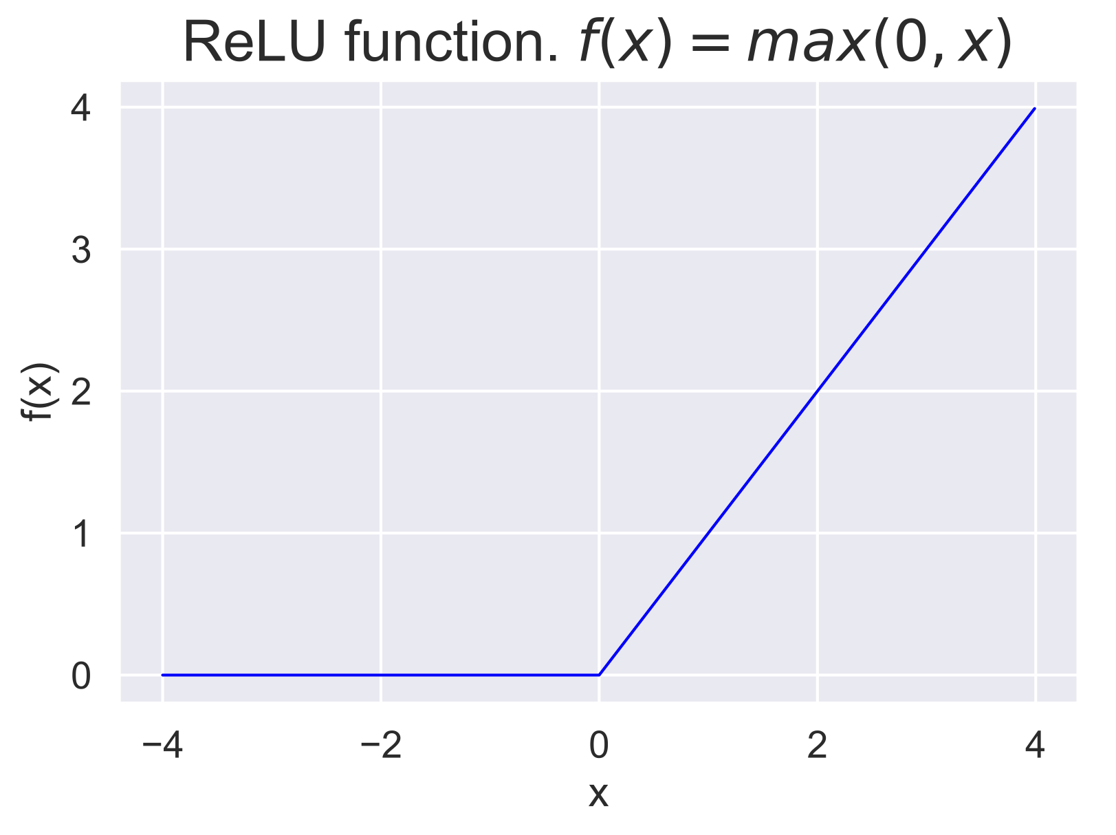
Figure 9: ReLU activation function

B.2 Linear activation function

Figure 10: Linear activation function

References

- [1] A. Saxena, K. Goebel, PHM08 challenge data set, https://ti.arc.nasa.gov/tech/dash/groups/pcoe/prognostic-data-repository/ (2008).
- [2] N. Z. Gebraeel, M. A. Lawley, R. Li, V. Parmeshwaran, Residual-life distributions from component degradation signals: A neural-network approach, IEEE Transactions on Industrial Electronics 51 (3) (2005) 150–172.
- [3] M. Zaidan, A. Mills, R. Harrison, Bayesian framework for aerospace gas turbine engine prognostics, in: IEEE (Ed.), Aerospace Conference, 2013, pp. 1–8.
- [4] Z. Zhao, L. Bin, X. Wang, W. Lu, Remaining useful life prediction of aircraft engine based on degradation pattern learning, Reliability Engineering & System Safety 164 (2017) 74–83.
- [5] J. Lee, F. Wu, W. Zhao, M. Ghaffari, L. Liao, D. Siegel, Prognostics and health management design for rotary machinery systems - reviews, methodology and applications, Mechanical Systems and Signal Processing 42 (12) (2014) 314–334.
- [6] W. Yu, H. Kuffi, A new stress-based fatigue life model for ball bearings, Tribology Transactions 44 (1) (2001) 11–18.
- [7] J. Liu, G. Wang, A multi-state predictor with a variable input pattern for system state forecasting, Mechanical Systems and Signal Processing 23 (5) (2009) 1586–1599.
- [8] A. Mosallam, K. Medjaher, N. Zerhouni, Nonparametric time series modelling for industrial prognostics and health management, The International Journal of Advanced Manufacturing Technology 69 (5) (2013) 1685–1699.
- [9] M. Pecht, Jaai, A prognostics and health management roadmap for information and electronics rich-systems, Microelectronics Reliability 50 (3) (2010) 317–323.
- [10] J. Liu, M. Wang, Y. Yang, A data-model-fusion prognostic framework for dynamic system state forecasting, Engineering Applications of Artificial Intelligence 25 (4) (2012) 814–823.
- [11] Y. Qian, R. Yan, R. X. Gao, A multi-time scale approach to remaining useful life prediction in rolling bearing, Mechanical Systems and Signal Processing 83 (2017) 549–567.
- [12] T. Benkedjouh, K. Medjaher, N. Zerhouni, S. Rechak, Remaining useful life estimation based on nonlinear feature reduction and support vector regression, Engineering Applications of Artificial Intelligence 26 (7) (2013) 1751–1760.
- [13] M. Dong, D. He, A segmental hidden semi-markov model (HSMM)-based diagnostics and prognostics framework and methodology, Mechanical Systems and Signal Processing 21 (5) (2007) 2248–2266.
- [14] X. Li, Q. Ding, J. Sun, Remaining useful life estimation in prognostics using deep convolution neural networks, Reliability Engineering and System Safety 172 (2018) 1–11.
- [15] J. Z. Sikorska, M. Hodkiewicz, L. Ma, Prognostic modelling options for remaining useful life estimation by industry, Mechanical Systems and Signal Processing 25 (5) (2011) 1803–1836.
- [16] P. Lim, C. K. Goh, K. C. Tan, A time-window neural networks based framework for remaining useful life estimation, in: Proceedings International Joint Conference on Neural Networks, 2016, pp. 1746–1753.
- [17] A. Saxena, K. Goebel, D. Simon, N. Eklund, Damage propagation modeling for aircraft engine run-to-failure simulation, in: International Conference On Prognostics and Health Management, IEEE, 2008, pp. 1–9.
- [18] E. Ramasso, Investigating computational geometry for failure prognostics, International Journal of Prognostics and Health Management 5 (1) (2014) 1–18.
-
[19]
D. Laredo, X. Chen, O. Schütze, J. Q. Sun,
ANN-EA for RUL
estimation, source code, [Online] (2018).
URL https://github.com/dlaredo/NASA_RUL_-CMAPS- - [20] P. Bühlmann, G. S., Statistics for High Dimensional Data. Methods, Theory and Applications, Springer, 2011.
- [21] C. Kong, S. Lucey, Take it in your stride: Do we need striding in CNNs?, arXiv:1712.02502 (2017).
- [22] R. Storn, K. Price, Differential evolution: A simple and efficient heuristic for global optimization over continuous spaces, Journal of Global Optimization 11 (4) (1997) 341–359.
-
[23]
E. Jones, T. Oliphant, P. Peterson, et al.,
SciPy: Open source scientific tools for
Python, [Online; accessed 06/2018] (2001).
URL http://www.scipy.org/ - [24] D. Engelbrecht, Computational Intelligence: An Introduction, Willey, 2007.
- [25] Y. Peng, H. Wang, J. Wang, D. Liu, X. Peng, A modified echo state network based remaining useful life estimation approach, in: IEEE Conference on Prognostics and Health Management, 2012, pp. 1–7.
- [26] C. Louen, S. X. Ding, C. Kandler, A new framework for remaining useful life estimation using support vector machine classifier, in: Conference on Control and Fault-Tolerant Systems, 2013, pp. 228–233.
- [27] C. Zhang, P. Lim, A. Qin, K. Tan, Multiobjective deep belief networks ensemble for remaining useful life estimation in prognostics, IEEE Transactions on Neural Networks and Learning Systems 99 (2016) 1–13.
- [28] G. S. Babu, P. Zhao, X. Li, Deep convolutional neural network based regression approach for estimation of remaining useful life, in: S. I. Publishing (Ed.), 21st International Conference on Database Systems for Advanced Applications, 2016, pp. 214–228.
- [29] P. Malhotra, V. TV, A. Ramakrishnan, G. Anand, L. Vig, P. Agarwal, G. Shroff, Multi-sensor prognostics using an unsupervised health index based on lstm encoder-decoder, arXiv:1608.06154 (2016).