Task-Driven Modular Networks for Zero-Shot Compositional Learning

Abstract

One of the hallmarks of human intelligence is the ability to compose learned knowledge into novel concepts which can be recognized without a single training example. In contrast, current state-of-the-art methods require hundreds of training examples for each possible category to build reliable and accurate classifiers. To alleviate this striking difference in efficiency, we propose a task-driven modular architecture for compositional reasoning and sample efficient learning. Our architecture consists of a set of neural network modules, which are small fully connected layers operating in semantic concept space. These modules are configured through a gating function conditioned on the task to produce features representing the compatibility between the input image and the concept under consideration. This enables us to express tasks as a combination of sub-tasks and to generalize to unseen categories by reweighting a set of small modules. Furthermore, the network can be trained efficiently as it is fully differentiable and its modules operate on small sub-spaces. We focus our study on the problem of compositional zero-shot classification of object-attribute categories. We show in our experiments that current evaluation metrics are flawed as they only consider unseen object-attribute pairs. When extending the evaluation to the generalized setting which accounts also for pairs seen during training, we discover that naïve baseline methods perform similarly or better than current approaches. However, our modular network is able to outperform all existing approaches on two widely-used benchmark datasets.

1 Introduction

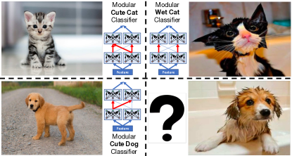
Figure 1: We investigate how to build a classifier on-the-fly, for a new concept (“wet dog”) given knowledge of related concepts (“cute dog”, “cute cat”, and “wet cat”). Our approach consists of a modular network operating in a semantic feature space. By rewiring its primitive modules, the network can recognize new structured concepts.

How can machines reliably recognize the vast number of possible visual concepts? Even simple concepts like “envelope” could, for instance, be divided into a seemingly infinite number of sub-categories, e.g., by size (large, small), color (white, yellow), type (plain, windowed), or condition (new, wrinkled, stamped). Moreover, it has frequently been observed that visual concepts follow a long-tailed distribution [26, 33, 30]. Hence, most classes are rare, and yet humans are able to recognize them without having observed even a single instance. Although a surprising event, most humans wouldn’t have trouble to recognize a “tiny striped purple elephant sitting on a tree branch”. For machines, however, this would constitute a daunting challenge. It would be impractical, if not impossible, to gather sufficient training examples for the long tail of all possible categories, even more so as current learning algorithms are data-hungry and rely on large amounts of labeled examples. How can we build algorithms to cope with this challenge?

One possibility is to exploit the compositional nature of the prediction task. While a machine may not have observed any images of “wrinkled envelope”, it may have observed many more images of “white envelope”, as well as “white paper” and “wrinkled paper”. If the machine is capable of compositional reasoning, it may be able to transfer the concept of being “wrinkled” from “paper” to “envelope”, and generalize without requiring additional examples of actual “wrinkled envelope”.

One key challenge in compositional reasoning is contextuality. The meaning of an attribute, and even the meaning of an object, may be dependent on each other. For instance, how “wrinkled” modifies the appearance of “envelope” is very different from how it changes the appearance of “dog”. In fact, contextuality goes beyond semantic categories. The way “wrinkled” modifies two images of “dog” strongly depends on the actual input dog image. In other words, the model should capture intricate interactions between the image, the object and the attribute in order to perform correct inference. While most recent approaches [19, 20] capture the contextual relationship between object and attribute, they still rely on the original feature space being rich enough, as inference entails matching image features to an embedding vector of an object-attribute pair.

In this paper, we focus on the task of compositional learning, where the model has to predict the object present in the input image (e.g., “envelope”), as well as its corresponding attribute (e.g., “wrinkled”). We believe there are two key ingredients required: (a) learning high-level sub-tasks which may be useful to transfer concepts, and (b) capturing rich interactions between the image, the object and the attribute. In order to capture both these properties, we propose Task-driven Modular Networks (TMN).

First, we tackle the problem of transfer and re-usability by employing modular networks in the high-level semantic space of CNNs [14, 8]. The intuition is that by modularizing in the concept space, modules can now represent common high-level sub-tasks over which “reasoning” can take place: in order to recognize a new object-attribute pair, the network simply re-organizes its computation on-the-fly by appropriately reweighing modules for the new task. Apart from re-usability and transfer, modularity has additional benefits: (a) sample efficiency: transfer reduces to figuring out how to gate modules, as opposed to how to learn their parameters; (b) computational efficiency: since modules operate in smaller dimensional sub-spaces, predictions can be performed using less compute; and (c) interpretability: as modules specialize and similar computational paths are used for visually similar pairs, users can inspect how the network operates to understand which object-attribute pairs are deemed similar, which attributes drastically change appearance, etc. (§4.2).

Second, the model extracts features useful to assess the joint-compatibility between the input image and the object-attribute pair. While prior work [19, 20] mapped images in the embedding space of objects and attributes by extracting features only based on images, our model instead extracts features that depend on all the members of the input triplet. The input object-attribute pair is used to rewire the modular network to ultimately produce features invariant to the input pair. While in prior work the object and attribute can be extracted from the output features, in our model features are exclusively optimized to discriminate the validity of the input triplet.

Our experiments in §4.1 demonstrate that our approach outperforms all previous approaches under the “generalized” evaluation protocol on two widely used evaluation benchmarks. The use of the generalized evaluation protocol, which tests performance on both unseen and seen pairs, gives a more precise understanding of the generalization ability of a model [5]. In fact, we found that under this evaluation protocol baseline approaches often outperform the current state of the art. Furthermore, our qualitative analysis shows that our fully differentiable modular network learns to cluster together similar concepts and has intuitive interpretation. We will publicly release the code and models associated with this paper.

2 Related Work

Compositional zero-shot learning (CZSL) is a special case of zero-shot learning (ZSL) [21, 13]. In ZSL the learner observes input images and corresponding class descriptors. Classes seen at test time never overlap with classes seen at training time, and the learner has to perform a prediction of an unseen class by leveraging its class descriptor without any training image (zero-shot). In their seminal work, Chao et al. [5] showed that ZSL’s evaluation methodology is severely limited because it only accounts for performance on unseen classes, and they propose i) to test on both seen and unseen classes (so called “generaralized” setting) and ii) to calibrate models to strike the best trade-off between achieving a good performance on the seen set and on the unseen set. In our work, we adopt the same methodology and calibration technique, although alternative calibration techniques have also been explored in literature [4, 16]. The difference between our generalized CZSL (GCZSL) setting and generalized ZSL is that we predict not only an object id, but also its corresponding attribute. The prediction of such pair makes the task compositional as given $N$ objects and $M$ attributes, there are potentially $N*M$ possible pairs the learner could predict.

Most prior approaches to CZSL are based on the idea of embedding the object-attribute pair in image feature space [19, 20]. In our work instead, we propose to learn the joint compatibility [15] between the input image and the pair by learning a representation that depends on the input triplet, as opposed to just the image. This is potentially more expressive as it can capture intricate dependencies between image and object-attribute pair.

A major novelty compared to past work is also the use of modular networks. Modular networks can be interpreted as a generalization of hierarchical mixture of experts [10, 11, 6], where each module holds a distribution over all the modules at the layer below and where the gatings do not depend on the input image but on a task descriptor. These networks have been used in the past to speed up computation at test time [1] and to improve generalization for multi-task learning [17, 24], reinforcement learning [7], continual learning [28], visual question answering [2, 23], etc. but never for CZSL.

The closest approach to ours is the concurrent work by Wang et al. [32], where the authors factorize convolutional layers and perform a component-wise gating which depends on the input object-attribute pair, therefore also using a task driven architecture. This is akin to having as many modules as feature dimensions, which is a form of degenerate modularity since individual feature dimensions are unlikely to model high-level sub-tasks.

Finally, our gating network which modulates the computational blocks in the recognition network, can also be interpreted as a particular instance of meta-learning [27, 31], whereby the gating network predicts on-the-fly a subset of task-specific parameters (the gates) in the recognition network.

3 Approach

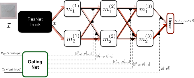
Figure 2: Toy illustration of the task-driven modular network (TMN). A pre-trained ResNet trunk extracts high level semantic representations of an input image. These features are then fed to a modular network (in this case, three layers with two modules each) whose blocks are gated (black triangle amplifiers) by a gating network. The gating network takes as input an object and an attribute id. Task driven features are then projected into a single scalar value representing the joint compatibility of the triplet (image, object and attrtibute). The overlaid red arrows show the strength of the gatings on each edge.

Consider the visual classification setting where each image $\mathcal{I}$ is associated with a visual concept $c$. The manifestation of the concepts $c$ is highly structured in the visual world. In this work, we consider the setting where images are the composition of an object (e.g., “envelope”) denoted by $c_{o}$, and an attribute (e.g., “wrinkled”) denoted by $c_{a}$; therefore, $c=(c_{o},c_{a})$. In a fully-supervised setting, classifiers are trained for each concept $c$ using a set of human-labelled images and then tested on novel images belonging to the same set of concepts. Instead, in this work we are interested in leveraging the compositional nature of the labels to extrapolate classifiers to novel concepts at test time, even without access to any training examples on these new classes (zero-shot learning).

More formally, we assume access to a training set $\mathcal{D}_{\text{train}}=\{(\mathcal{I}^{(k)},c^{(k)})~{}|~{}k=1,2,...,N_{\text{train}}\}$ consisting of image $\mathcal{I}$ labelled with a concept $c\in\mathcal{C}_{\text{train}}$, with $\mathcal{C}_{\text{train}}\subset\mathcal{C}_{o}\times\mathcal{C}_{a}=\{(c_{o},c_{a})~{}|~{}c_{o}\in\mathcal{C}_{o},c_{a}\in\mathcal{C}_{a}\}$ where $\mathcal{C}_{o}$ is the set of objects and $\mathcal{C}_{a}$ is the set of attributes.

In order to evaluate the ability of our models to perform zero-shot learning, we use a similar validation ($\mathcal{D}_{\text{val}}$) and test ($\mathcal{D}_{\text{test}}$) sets consisting of images labelled with concepts from $\mathcal{C}_{\text{val}}$ and $\mathcal{C}_{\text{test}}$, respectively. In contrast to a fully-supervised setting, validation and test concepts do not fully overlap with training concepts, i.e. $\mathcal{C}_{\text{val}}\backslash\mathcal{C}_{\text{train}}\neq\emptyset$, $\mathcal{C}_{\text{test}}\backslash\mathcal{C}_{\text{train}}\neq\emptyset$ and $\mathcal{C}_{\text{cal}}\cap\mathcal{C}_{\text{train}}\neq\emptyset$, $\mathcal{C}_{\text{test}}\cap\mathcal{C}_{\text{train}}\neq\emptyset$. Therefore, models trained to classify training concepts must also generalize to “unseen” concepts to successfully classify images in the validation and test sets. We call this learning setting, Generalized Zero-Shot Compositional learning, as both seen and unseen concepts appear in the validation and test sets. Note that this setting is unlike standard practice in prior literature where a common validation set is absent and only unseen pairs are considered in the test set [19, 20, 32].

In order to address this compositional zero-shot learning task, we propose a Task-driven Modular Network (TMN) which we describe next.

3.1 Task-Driven Modular Networks (TMN)

The basis of our architecture design is a scoring model [15] of the joint compatibility between image, object and attribute. This is motivated by the fact that each member of the triplet exhibits intricate dependencies with the others, i.e. how an attribute modifies appearance depends on the object category as well as the specific input image. Therefore, we consider a function that takes as input the whole triplet and extracts representations of it in order to assign a compatibility score. The goal of training is to make the model assign high score to correct triplets (using the provided labeled data), and low score to incorrect triplets. The second driving principle is modularity. Since the task is compositional, we add a corresponding inductive bias by using a modular network. During training the network learns to decompose each recognition task into sub-tasks that can then be combined in novel ways at test time, consequently yielding generalizeable classifiers.

The overall model is outlined in Fig. 2. It consists of two components: a gating model $\mathcal{G}$ and a feature extraction model $\mathcal{F}$. The latter $\mathcal{F}$ consists of a set of neural network modules, which are small, fully-connected layers but could be any other parametric differentiable function as well. These modules are used on top of a standard ResNet pre-trained trunk. Intuitively, the ResNet trunk is used to map the input image $\mathcal{I}$ to a semantic concept space where higher level “reasoning” can be performed. We denote the mapped $\mathcal{I}$ in such semantic space with $x$. The input to each module is a weighted-sum of the outputs of all the modules at the layer below, with weights determined by the gating model $\mathcal{G}$, which effectively controls how modules are composed.

Let $L$ be the number of layers in the modular part of $\mathcal{F}$, $M^{(i)}$ be the number of modules in the $i$-th layer, $m^{(i)}_{j}$ be $j$-th module in layer $i$ and $x^{(i)}_{j}$ be the input to each module, then we have:

$$x^{(i)}_{j}=\sum_{k=1}^{M^{(i-1)}}g^{(i)}_{k\rightarrow j}*o^{(i-1)}_{k},$$ (1)

where $*$ is the scalar-vector product, the output of the $k$-th module in layer $(i-1)$ is $o^{(i-1)}_{k}=m^{(i-1)}_{k}\big{[}x^{(i-1)}_{k}\big{]}$ and the weight on the edge between $m^{(i-1)}_{k}$ and $m^{(i)}_{j}$ is denoted by $g^{(i)}_{k\rightarrow j}\in\mathbb{R}$. The set of gatings $g=\{g^{(i)}_{k\rightarrow j}~{}|~{}i\in[1,L],j\in[1,M^{(i)}],k\in[1,M^{(i-1)}]\}$ jointly represent how modules are composed for scoring a given concept.

The gating network $\mathcal{G}$ is responsible for producing the set of gatings $g$ given a concept $c=(c_{o},c_{a})$ as input. $c_{o}$ and $c_{a}$ are represented as integer ids, and are then embedded using a learned lookup table. These embeddings are then concatenated and processed by a multilayer neural network which computes the gatings as:

$$\mathcal{G}(c)=[q^{(1)}_{1\rightarrow 1},q^{(1)}_{2\rightarrow 1},....q^{(L)}_{M^{(L-1)}\rightarrow M^{(L)}}],$$ (2)

$$g^{(i)}_{k\rightarrow j}=\frac{\exp[q^{(i)}_{k\rightarrow j}]}{\sum_{k^{\prime}=1}^{M^{(i-1)}}\exp[q^{(i)}_{k^{\prime}\rightarrow j}]}.$$ (3)

Therefore, all incoming gating values to a module are positive and sum to one.

The output of the feature extraction network $\mathcal{F}$ is a feature vector, $o^{(L)}_{1}$, which is linearly projected into a real value scalar to yield the final score, $s_{c}(\mathcal{I},(c_{o},c_{a}))$. This represents the compatibility of the input triplet, see Fig. 2.

3.2 Training & Testing

Our proposed training procedure involves jointly learning the parameters of both gating and feature extraction networks (without fine-tuning the ResNet trunk for consistency with prior work [19, 20]). Using the training set described above, for each sample image $\mathcal{I}$ we compute scores for all concepts $c=(c_{o},c_{a})\in\mathcal{C}_{\text{train}}$ and turn scores into normalized probabilities with a softmax: $p_{c}=\frac{\exp[s_{c}]}{\sum_{c^{\prime}\in C_{\text{train}}}\exp[s_{c^{\prime}}]}$. The standard (per-sample) cross-entropy loss is then used to update the parameters of both $\mathcal{F}$ and $\mathcal{G}$: ${\mathcal{L}(\mathcal{I},\hat{c})=-\log p_{\hat{c}}}$, if $\hat{c}$ is the correct concept.

In practice, computing the scores of all concepts may be computationally too expensive if $\mathcal{C}_{\text{train}}$ is large. Therefore, we approximate the probability normalization factor by sampling a random subset of negative candidates [3].

Finally, in order to encourage the model to generalize to unseen pairs, we regularize using a method we dubbed ConceptDrop. At each epoch, we choose a small random subset of pairs, exclude those samples and also do not consider them for negative pairs candidates. We cross-validate the size of the ConceptDrop subset for all the models.

At test time, given an image we score all pairs present in $\mathcal{C}_{\text{test}}\cup\mathcal{C}_{\text{train}}$, and select the pair yielding the largest score. However, often the model is not calibrated for unseen concepts, since the unseen concepts were not involved in the optimization of the model. Therefore, we could add a scalar bias term to the score of any unseen concept [5]. Varying the bias from very large negative values to very large positive values has the overall effect of limiting classification to only seen pairs or only unseen pairs respectively. Intermediate values strike a trade-off between the two.

4 Experiments

We first discuss datasets, metrics and baselines used in this paper. We then report our experiments on two widely used benchmark datasets for CZSL, and we conclude with a qualitative analysis demonstrating how TMN operates. Data and code will be made publicly available.

Datasets

We considered two datasets. The MIT-States dataset [9] has 245 object classes, 115 attribute classes and about 53K images. On average, each object is associated with 9 attributes. There are diverse object categories, such as “highway” and “elephant”, and there is also large variation in the attributes, e.g. “mossy” and “diced” (see Fig. 4 and 7 for examples). The training set has about 30K images belonging to 1262 object-attribute pairs (the seen set), the validation set has about 10K images from 300 seen and 300 unseen pairs, and the test set has about 13K images from 400 seen and 400 unseen pairs.

The second dataset is UT-Zappos50k [34] which has 12 object classes and 16 attribute classes, with a total of about 33K images. This dataset consists of different types of shoes, e.g. “rubber sneaker”, “leather sandal”, etc. and requires fine grained classification ability. This dataset has been split into a training set containing about 23K images from 83 pairs (the seen pairs), a validation set with about 3K images from 15 seen and 15 unseen pairs, and a test set with about 3K images from 18 seen and 18 unseen pairs.

The splits of both datasets are different from those used in prior work [20, 19], now allowing fair cross-validation of hyperparameters and evaluation in the generalized zero-shot learning setting. We will make the splits publicly available to facilitate easy comparison for future research.

Architecture and Training Details

The common trunk of the feature extraction network is a ResNet-18 [8] pretrained on ImageNet [25] which is not finetuned, similar to prior work [19, 20]. Unless otherwise stated, our modular network has 24 modules in each layer. Each module operates in a 16 dimensional space, i.e. the dimensionality of $x^{(i)}_{j}$ and $o^{(i)}_{j}$ in eq. 1 is 16. Finally, the gating network is a 2 layer neural network with 64 hidden units. The input lookup table is initialized with Glove word embeddings [22] as in prior work [20]. The network is optimized by stochastic gradient descent with ADAM [12] with minibatch size equal to 256. All hyper-parameters are found by cross-validation on the validation set (see §4.1.1 for robustness to number of layers and number of modules).

Baselines

We compare our task-driven modular network against several baseline approaches. First, we consider the RedWine method [19] which represents objects and attributes via SVM classifier weights in CNN feature space, and embeds these parameters in the feature space to produce a composite classifier for the (object, attribute) pair. Next, we consider LabelEmbed+ [20] which is a common compositional learning baseline. This model involves embedding the concatenated (object, attribute) Glove word vectors and the ResNet feature of an image, into a joint feature space using two separate multilayer neural networks. Finally, we consider the recent AttributesAsOperators approach [20], which represents the attribute with a matrix and the object with a vector. The product of the two is then multiplied by a projection of the ResNet feature space to produce a scalar score of the input triplet. All methods use the same ResNet features as ours. Note that architectures from [19, 20] have more parameters compared to our model. Specifically, RedWine, LabelEmbed+ and AttributesAsOperators have approximately 11, 3.5 and 38 times more parameters (excluding the common ResNet trunk) than the proposed TMN.

Metrics

We follow the same evaluation protocol introduced by Chao et al. [5] in generalized zero-shot learning, as all prior work on CZSL only tested performance on unseen pairs without controlling accuracy on seen pairs. Most recently, Nagarajan et al. [20] introduced an “open world” setting whereby both seen and unseen pairs are considered during scoring but only unseen pairs are actually evaluated. As pointed out by Chao et al. [5], this methodology is flawed because, depending on how the system is trained, seen pairs can evaluate much better than unseen pairs (typically when training with cross-entropy loss that induces negative biases for unseen pairs) or much worse (like in [20] where unseen pairs are never used as negatives when ranking at training time, resulting in an implicit positive bias towards them). Therefore, for a given value of the calibration bias (a single scalar added to the score of all unseen pairs, see §3.2), we compute the accuracy on both seen and unseen pairs, (recall that our validation and test sets have equal number of both). As we vary the value of the calibration bias we draw a curve and then report its area (AUC) later to describe the overall performance of the system.

For the sake of comparison to prior work, we also report the “closed-world” accuracy [20, 19], i.e. the accuracy of unseen pairs when considering only unseen pairs as candidates.

4.1 Quantitative Analysis

Table 1: AUC (multiplied by 100) for MIT-States and UT-Zappos. Columns correspond to AUC computed using precision at k=1,2,3.

	MIT-States						UT-Zappos
	Val AUC			Test AUC			Val AUC			Test AUC
Model    Top $k\rightarrow$	1	2	3	1	2	3	1	2	3	1	2	3
AttrAsOp [20]	2.5	6.2	10.1	1.6	4.7	7.6	21.5	44.2	61.6	25.9	51.3	67.6
RedWine [19]	2.9	7.3	11.8	2.4	5.7	9.3	30.4	52.2	63.5	27.1	54.6	68.8
LabelEmbed+ [20]	3.0	7.6	12.2	2.0	5.6	9.4	26.4	49.0	66.1	25.7	52.1	67.8
TMN (ours)	3.5	8.1	12.4	2.9	7.1	11.5	36.8	57.1	69.2	29.3	55.3	69.8

Table 2: Best seen and unseen accuracies, and best harmonic mean of the two. See companion Fig. 3 for the operating points used.

	MIT-States			UT-Zappos
Model	Seen (○)	Unseen ($\times$)	HM ($\blacklozenge$)	Seen	Unseen	HM
AttrAsOp	14.3	17.4	9.9	59.8	54.2	40.8
RedWine	20.7	17.9	11.6	57.3	62.3	41.0
LabelEmbed+	15.0	20.1	10.7	53.0	61.9	40.6
TMN (ours)	20.2	20.1	13.0	58.7	60.0	45.0

The main results of our experiments are reported in Tab. 1. First, on both datasets we observe that TMN performs consistently better than the other tested baselines. Second, the overall absolute values of AUC are fairly low, particularly on the MIT-States dataset which has about 2000 attribute-object pairs and lots of potentially valid pairs for a given image due to the inherent ambiguity of the task. Third, the best runner up method is RedWine [19], suprisingly followed closely by the LabelEmbed+ baseline [20].

The importance of using the generalized evaluation protocol becomes apparent when looking directly at the seen-unseen accuracy curve, see Fig. 3. This shows that as we increase the calibration bias we improve classification accuracy on unseen pairs but decrease the accuracy on seen pairs. Therefore, comparing methods at different operating points is inconclusive. For instance, RedWine yields the best seen pair accuracy of 20.7% when the unseen pair accuracy is 0%, compared to our approach which achieves 20.2%, but this is hardly a useful operating point.

For the sake of comparison, we also report the best seen accuracy, the best unseen accuracy and the best harmonic mean of the two for all these methods in Tab. 2. Although our task-driven modular network may not always yield the best seen/unseen accuracy, it significantly improves the harmonic mean, indicating an overall better trade-off between the two accuracies.

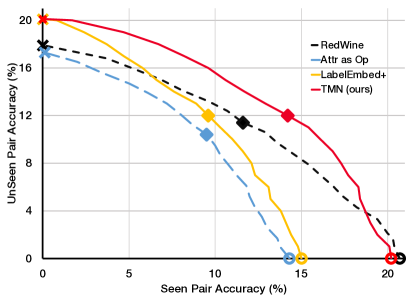
Figure 3: Unseen-Seen accuracy curves on MIT-States dataset. Prior work [20] reported unseen accuracy at different (unknown) values of seen accuracy, making comparisons inconclusive. Instead, we report AUC values [5], see Tab. 1.

Our model not only performs better in terms of AUC but also trains efficiently. We observed that it learns from fewer updates during training. For instance, on the MIT-States datatset, our method reaches the reported AUC of 3.5 within 4 epochs. In contrast, embedding distance based approaches such as AttributesAsOperators [20] and LabelEmbed+ require between 400 to 800 epochs to achieve the best AUC values using the same minibatch size. This is partly attributed to the processing of a larger number of negatives candidate pairs in each update of TMN(see §3.2). The modular structure of our network also implies that for a similar number of hidden units, the modular feature extractor has substantially fewer parameters compared to a fully-connected network. A fully-connected version of each layer would have $D^{2}$ parameters, if $D$ is the number of input and output hidden units. Instead, our modular network has $M$ blocks, each with $(\frac{D}{M})^{2}$ parameters. Overall, one layer of the modular network has $D^{2}/(M*(\frac{D}{M})^{2})=M$ times less parameters (which is also the amount of compute saved). See the next section for further analogies with fully connected layers.

4.1.1 Ablation Study

Table 3: Ablation study: Top-1 valid. AUC; see §4.1.1 for details.

Model	MIT-States	UT-Zappos
TMN	3.5	36.8
a) without task driven gatings	3.2	32.7
b) like a) & no joint extraction	0.8	20.1
c) without ConceptDrop	3.3	35.7

Table 4: AUC(*100) on validaton set of MIT-States varying the number of modules per layer and the number of layers.

	Modules
Layers	12	18	24	30
1	1.86	2.14	2.50	2.51
3	3.23	3.44	3.51	3.44
5	3.48	3.31	3.24	3.19

In our first control experiment we assessed the importance of using a modular network by considering exactly the same architecture with two modifications. First, we learn a common set of gatings for all the concepts; henceforth, removing the task-driven modularity. And second, we feed the modular network with the concatenation of the ResNet features and the object-attribute pair embedding; henceforth, retaining the joint modeling of the triplet. To better understand this choice, consider the transformation of layer $i$ of the modular network in Fig. 2 which can be equivalently rewritten as:

$$\left[\begin{array}[]{c}o^{(i)}_{1}\\ o^{(i)}_{2}\end{array}\right]=\mbox{ReLU}(\left[\begin{array}[]{cc}g^{(i)}_{1\rightarrow 1}m^{(i)}_{1}&g^{(i)}_{2\rightarrow 1}m^{(i)}_{1}\\ g^{(i)}_{1\rightarrow 2}m^{(i)}_{2}&g^{(i)}_{2\rightarrow 2}m^{(i)}_{2}\end{array}\right]*\left[\begin{array}[]{c}o^{(i-1)}_{1}\\ o^{(i-1)}_{2}\end{array}\right])$$

assuming each square block $m^{(i)}_{j}$ is a ReLU layer. In a task driven modular network, gatings depend on the input object-attribute pair, while in this ablation study we use gatings agnostic to the task, as these are still learned but shared across all tasks. Each layer is a special case of a fully connected layer with a more constrained parameterization. This is the baseline shown in row a) of Tab. 3. On both datasets performance is deteriorated showing the importance of using task driven gates. The second baseline shown in row b) of Tab. 3, is identical to the previous one but we also make the features agnostic to the task by feeding the object-attribute embedding at the output (as opposed to the input) of the modular network. This is similar to LabelEmbed+ baseline of the previous section, but replacing the fully connected layers with the same (much more constrained) architecture we use in our TMN (without task-driven gates). In this case, we can see that performance drastically drops, suggesting the importance of extracting joint representations of input image and object-attribute pair. The last row c) assesses the contribution to the performance of the ConceptDrop regularization, see §3.2. Without it, AUC has a small but significant drop.

Finally, we examine the robustness to the number of layers and modules per layer in Tab. 4. Except when the modular network is very shallow, AUC is fairly robust to the choice of these hyper-parameters.

4.2 Qualitative Analysis

Table 5: Edge analysis. Example of the top 3 object-attribute pairs (rows) from MIT-States dataset that respond most strongly on 6 edges (columns) connecting blocks in the modular network.

dry river	tiny animal	cooked pasta	unripe pear	old city
dry forest	small animal	raw pasta	unripe fig	ancient city
dry stream	small snake	steaming pasta	unripe apple	old town

Table 6: Module analysis. Example of the top 3 object-attribute pairs (rows) for 6 randomly chosen modules (columns) according to the sum of outgoing edge weights in each pair’s gating.

dark fire	large tree	wrinkled dress	small elephant	pureed soup
dark ocean	small tree	ruffled dress	young elephant	large pot
dark cloud	mossy tree	ruffled silk	tiny elephant	thick soup

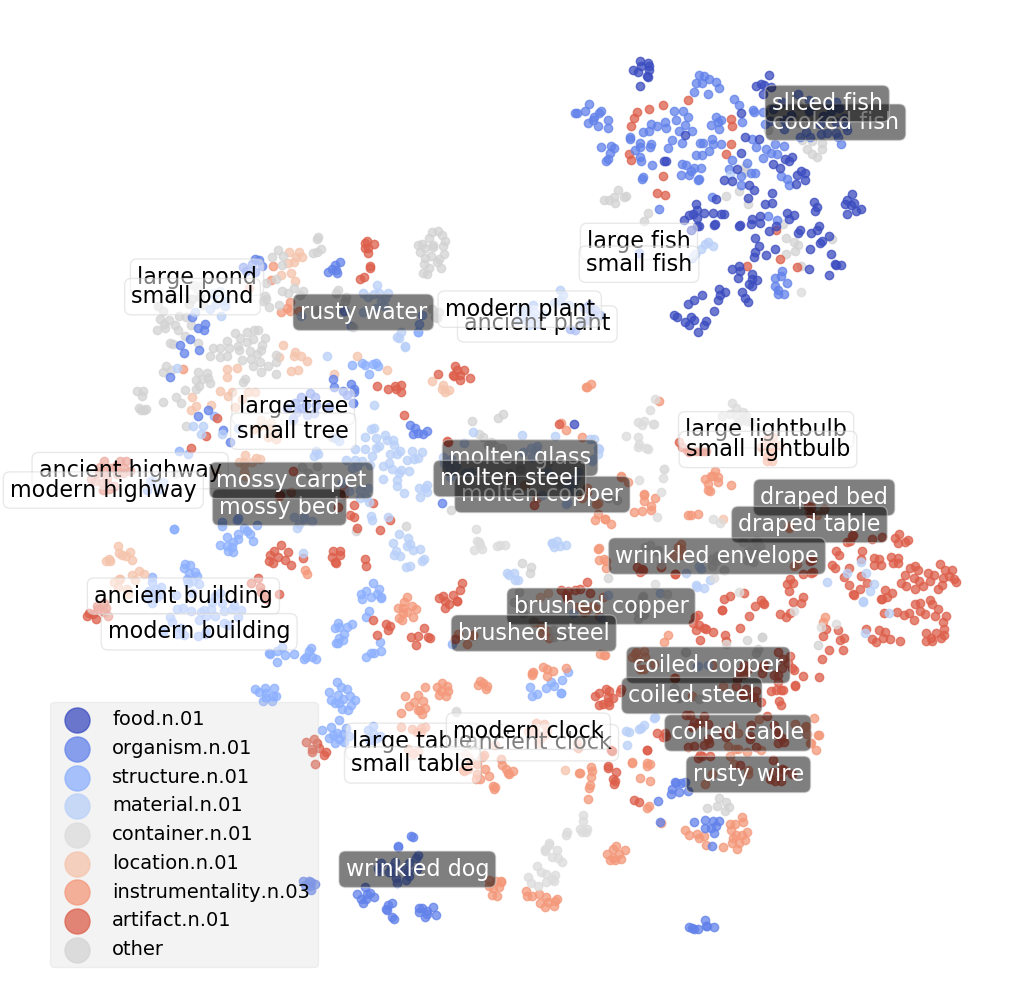
Figure 4: t-SNE embedding of Attribute-Object gatings on MIT-States dataset. Colors indicate high-level WordNet categories of objects. Pairs tagged with text boxes that have white background, indicate examples where changing the attribute results in similar gatings (e.g., large/small table); conversely, pairs in black background indicate examples where the change of attribute/object leads to very dissimilar gatings (e.g., molten/brushed/coil steel, rusty water/rusty wire).

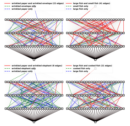
Figure 5: Examples of task driven topologies learned in TMN. Only edges whose associated weight is within 3% of the highest weight for that edge are displayed. At the bottom the source features $x$, at the top the module projecting down to a single scalar scoring value. Each subplot compares the gatings of two object-attribute pairs. The red edges are the edges that are common between the two pairs. The green and the blue segments are edges acttive only in one of the two pairs. Left: Examples of two sets of pairs all sharing the same attribute, “wrinkled”. Right: Examples of two sets of pairs all sharing the same object, “fish”. Top: examples of visually similar pairs. Bottom: example of visually dissimilar pairs (resulting in less overlapping graphs).

Task-driven modular networks are appealing not only for their performance but also because they are easy to interpret. In this section, we explore simple ways to visualize them and inspect their inner workings. We start by visualizing the learned gatings in three ways. First, we look at which object-attribute pair has the largest gating value on a given edge of the modular network. Tab. 5 shows some examples indicating that visually similar pairs exhibit large gating values on the same edge of the computational graph. Similarly, we can inspect the blocks of the modular architecture. We can easily do so by associating a module to those pairs that have largest total outgoing gatings. This indicates how much a module effects the next layer for the considered pair. As shown in Tab. 6, we again find that modules take ownership for explaining specific kinds of visually similar object-attribute pairs. A more holistic way to visualize the gatings is by embedding all the gating values associated with an object-attribute pair in the 2 dimensional plane using t-SNE [29], as shown in Fig. 4. This visualization shows that the gatings are mainly organized by visual similarity. Within this map, there are smaller clusters that correspond to the same object with various attributes. However, there are several exceptions to this, as there are instances where the attribute greatly changes the visual appearance of the object (“coiled steel” VS “molten steel”, see other examples highlighted with dark tags), for instance. Likewise, pairs sharing the same attribute may be located in distant places if the object is visually dissimilar (“rusty water” VS ”rusty wire”). The last gating visualization is through the topologies induced by the gatings, as shown in Fig. 5, where only the edges with sufficiently large gating values are shown. Overall, the degree of edge overlap between object-attribute pairs strongly depends on their visual similarity.

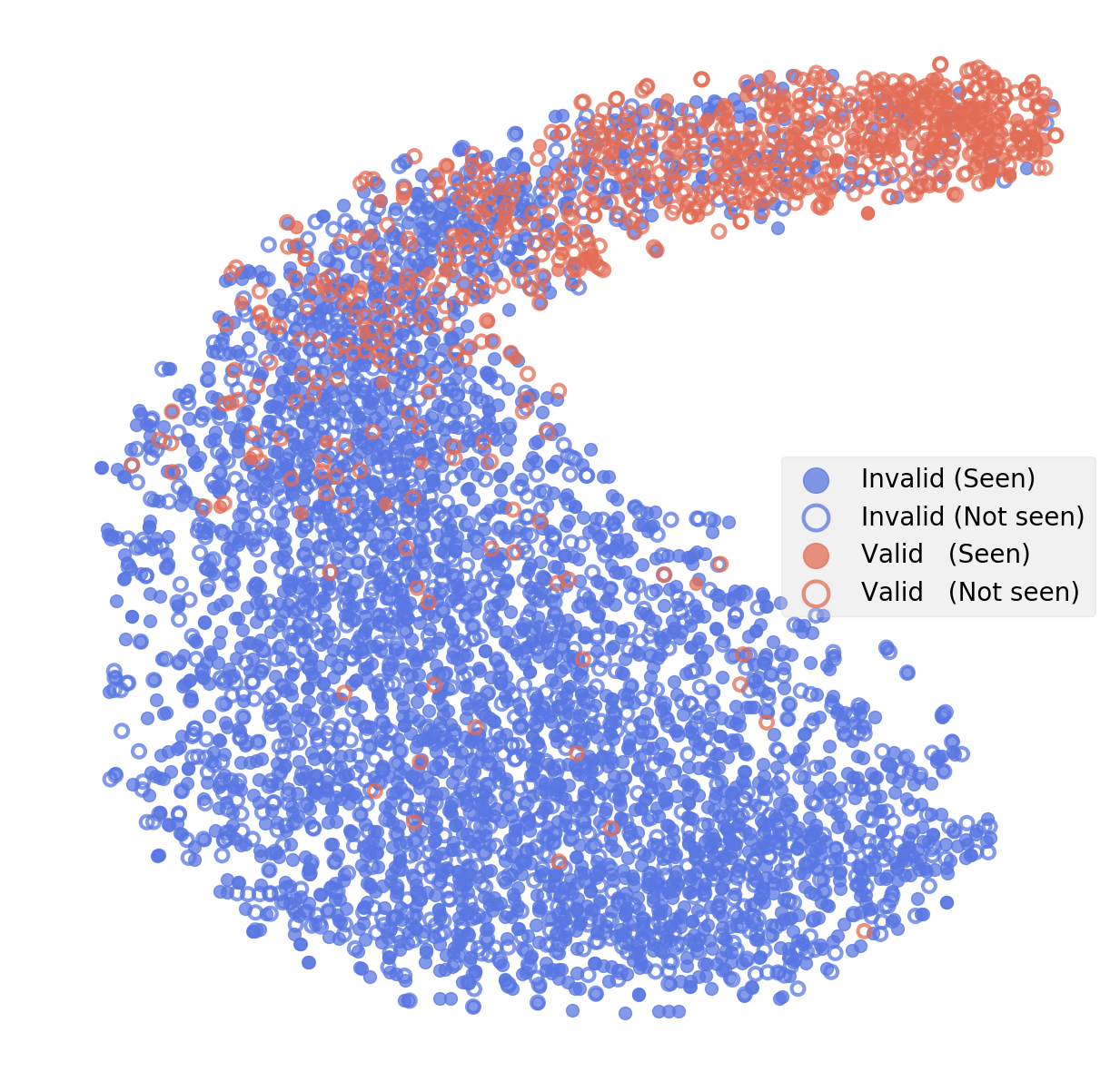
Figure 6: t-SNE embedding of the output features (just before the last linear projection) on MIT-States dataset. Red markers show valid (image, object, attribute) triplets (from either seen or unseen pairs), while blue markers show invalid triplets.

Besides gatings and modules, we also visualized the task-driven visual features $o^{(L)}_{1}$, just before the last linear projection layer, see Fig. 2. The map in Fig. 6 shows that valid (image, object, attribute) triplets are well clustered together, while invalid triplets are nicely spread on one side of the plane. This is quite different than the feature organization found by methods that match concept embeddings in the image feature space [20, 19], which tend to be organized by concept. While TMN extracts largely task-invariant representations using a task-driven architecture, they produce representations that contain information about the task using a task-agnostic architecture. TMN places all valid triplets on a tight cluster because the shared top linear projection layer is trained to discriminate between valid and invalid triplets (as opposed to different types of concepts).

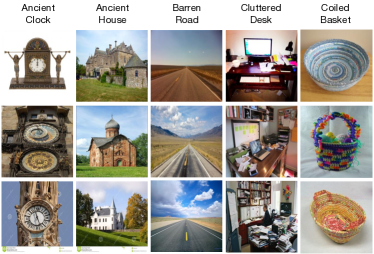
Figure 7: Example of image retrievals from the test set when querying an unseen pair (title of each column).

Finally, Fig. 7 shows some retrieval results. Given a query of an unseen object-attribute pair, we rank all images from the test set (which contains both seen and unseen pairs), and return those images that rank the highest. The model is able to retrieve relevant images despite not having been exposed to these concepts during training.

5 Conclusion

The distribution of highly structured visual concepts is very heavy tailed in nature. Improvement in sample efficiency of our current models is crucial, since labeled data will never be sufficient for concepts in the tail of the distribution. A promising way to attack this problem is to leverage the intrinsic compositionality of the label space. In this work, we investigate this avenue of research using the Zero-Shot Compositional Learning task as a use case. Our first contribution is a novel architecture: TMN, which outperforms all the baseline approaches we considered. There are two key ideas behind its design. First, the joint processing of input image, object and attribute to account for contextuality. And second, the use of a modular network with gatings dependent on the input object-attribute pair. Our second contribution is to advocate for the use of the generalized evaluation protocol which not only tests accuracy on unseen concepts but also seen concepts. Our experiments show that TMN provides better performance, while being efficient and interpretable. In future work, we will explore other gating mechanisms and applications in other domains.

6 Acknowledgements

We would like to thank Ishan Misra, Ramakrishna Vedantam and Xiaolong Wang for the discussions and feedback that helped us in this work.

Appendix A Hyperparameter tuning

The results we reported in the main paper were obtaining using the best hyper-parameters found on the validation set. We used the same cross-validation procedure for all methods, including ours. Here, we present the ranges of hyper-parameters used in the grid-search and the selected values.

A.1 Task Driven Modular Networks

Hyper-parameter values:

• Feature extractor learning rates: 0.1, 0.01, 0.001, 0.0001 (chosen: 0.001)

• Gating network learning rates: 0.1, 0.01, 0.001, 0.0001 (chosen: 0.01)

• Number of sampled sampled negatives for Eq 3: for MIT States 200, 400, 600 (chosen: 600), for UT-Zappos we choose all negatives

• Batch size: 64, 128, 256, 512 (chosen: 256)

• Fraction of train concepts dropped in ConceptDrop: 0%, 5%, 10%, 20% (chosen: 5%)

• Number of modules per layer: 12, 18, 24, 30 (chosen: 24)

• Output dimensions of each module: 8, 16 (chosen: 16)

• Number of layers: 1, 2, 3, 5 (chosen: 3 for MIT States, 2 for UT-Zappos)

A.2 LabelEmbed+

Hyper-parameter values:

• Learning rates: 0.1, 0.01, 0.001, 0.0001 (chosen: 0.0001 for MIT States, 0.001 for UT-Zappos)

• Batch size: 64, 128, 256, 512 (chosen: 512)

• Fraction of train concepts dropped in ConceptDrop: 0%, 5%, 10%, 20% (chosen: 5%)

A.3 RedWine

Hyper-parameter values:

• Learning rates: 0.1, 0.01, 0.001, 0.0001 (chosen: 0.01)

• Batch size: 64, 128, 256, 512 (chosen: 256 for MIT States, 512 for UT-Zappos)

• Fraction of train concepts dropped in ConceptDrop: 0%, 5%, 10%, 20% (chosen: 0%)

A.4 Attributes as Operators

Hyper-parameter values:

• Fraction of train concepts dropped in ConceptDrop: 0%, 5%, 10%, 20% (chosen: 5%)

Learning rate, batch size, regularization weights chosen from the original paper and executed using the implementation at: https://github.com/Tushar-N/attributes-as-operators.

2. Additional Topology Visualizations

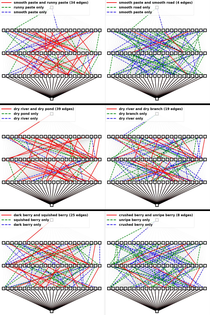
Figure 8: Additional Examples of task driven topologies learned in TMN (similar to Figure 5 of the main text).

References

- [1] K. Ahmed and L. Torresani. Maskconnect: Connectivity learning by gradient descent. In Proceedings of European Conference on Computer Vision (ECCV), 2018.
- [2] J. Andreas, M. Rohrbach, T. Darrell, and D. Klein. Deep compositional question answering with neural module networks. In Proceedings of IEEE Conference on Computer Vision and Pattern Recognition (CVPR), 2016.
- [3] Y. Bengio and J.-S. Senecal. Quick training of probabilistic neural nets by importance sampling. In Proceedings of the International Conference on Artificial Intelligence and Statistics (AISTATS), 2003.
- [4] Y. L. Cacheux, H. L. Borgne, and M. Crucianu. From classical to generalized zero-shot learning: a simple adaptation process. In Proceedings of the 25th International Conference on MultiMedia Modeling, 2019.
- [5] W.-L. Chao, S. Changpinyo, B. Gong, and F. Sha. An empirical study and analysis of generalized zero-shot learning for object recognition in the wild. In Proceedings of European Conference on Computer Vision (ECCV), 2016.
- [6] D. Eigen, I. Sutskever, and M. Ranzato. Learning factored representations in a deep mixture of experts. In Workshop at the International Conference on Learning Representations, 2014.
- [7] C. Fernando, D. Banarse, C. Blundell, Y. Zwols, D. Ha, A. A. Rusu, A. Pritzel, and D. Wierstra. Pathnet: Evolution channels gradient descent in super neural networks. arXiv:1701.08734, 2017.
- [8] K. He, X. Zhang, S. Ren, and J. Sun. Deep residual learning for image recognition. In Proceedings of IEEE Conference on Computer Vision and Pattern Recognition (CVPR), 2016.
- [9] P. Isola, J. Lim, and E. Adelson. Discovering states and transformations in image collections. In Proceedings of IEEE Conference on Computer Vision and Pattern Recognition (CVPR), 2015.
- [10] R. A. Jacobs, M. I. Jordan, S. Nowlan, and G. E. Hinton. Adaptive mixtures of local experts. Neural Computation, 3:1––12, 1991.
- [11] M. I. Jordan and R. A. Jacobs. Hierarchical mixtures of experts and the em algorithm. In International Joint Conference on Neural Networks, 1993.
- [12] D. Kingma and J. Ba. Adam: A method for stochastic optimization. In Proceedings of the International Conference on Learning Representations (ICLR), 2014.
- [13] C. H. Lampert, H. Nickisch, and S. Harmeling. Attribute-based classification for zero-shot visual object categorization. IEEE TPAMI, 36(3):453––465, 2014.
- [14] Y. LeCun, L. Bottou, Y. Bengio, and P. Haffner. Gradient-based learning applied to document recognition. Proceedings of the IEEE, 86(11):2278–2324, 1998.
- [15] Y. LeCun, S. Chopra, R. Hadsell, M. Ranzato, and F. Huang. A tutorial on energy-based learning. In G. Bakir, T. Hofman, B. Schölkopf, A. Smola, and B. Taskar, editors, Predicting Structured Data. MIT Press, 2006.
- [16] S. Liu, M. Long, J. Wang, and M. I. Jordan. Generalized zero-shot learning with deep calibration network. In Advances in Neural Information Processing Systems (NIPS), 2018.
- [17] E. Meyerson and R. Miikkulainen. Beyond shared hierarchies: Deep multitask learning through soft layer ordering. In Proceedings of the International Conference on Learning Representations (ICLR), 2018.
- [18] T. Mikolov, K. Chen, G. Corrado, and J. Dean. Efficient estimation of word representations in vector space. CoRR, abs/1301.3781, 2013.
- [19] I. Misra, A. Gupta, and M. Hebert. From red wine to red tomato: Composition with context. In Proceedings of IEEE Conference on Computer Vision and Pattern Recognition (CVPR), 2017.
- [20] T. Nagarajan and K. Grauman. Attributes as operators: Factorizing unseen attribute-object compositions. In Proceedings of European Conference on Computer Vision (ECCV), 2018.
- [21] M. Palatucci, D. Pomerleau, G. E. Hinton, and T. M. Mitchell. Zero-shot learning with semantic output codes. In Advances in Neural Information Processing Systems (NIPS), 2009.
- [22] J. Pennington, R. Socher, and C. Manning. Glove: Global vectors for word representation. In Proceedings of the Conference on Empirical Methods in Natural Language Processing (EMNLP), 2014.
- [23] E. Perez, F. Strub, H. de Vries, V. Dumoulin, and A. Courville. Film: Visual reasoning with a general conditioning layer. In AAAI, 2018.
- [24] C. Rosenbaum, T. Klinger, and M. Riemer. Routing networks: Adaptive selection of non-linear functions for multi-task learning. In Proceedings of the International Conference on Learning Representations (ICLR), 2018.
- [25] O. Russakovsky, J. Deng, H. Su, J. Krause, S. Satheesh, S. Ma, Z. Huang, A. Karpathy, A. Khosla, M. Bernstein, et al. Imagenet large scale visual recognition challenge. arXiv preprint arXiv:1409.0575, 2014.
- [26] R. Salakhutdinov, A. Torralba, and J. Tenenbaum. Learning to share visual appearance for multiclass object detection. In CVPR 2011, pages 1481–1488. IEEE, 2011.
- [27] J. Schmidhuber. Evolutionary principles in self-referential learning, or on learning how to learn: the meta-meta-… hook. PhD thesis, Technische Universität München, 1987.
- [28] L. Valkov, D. Chaudhari, A. Srivastava, C. Sutton, and S. Chaudhuri. Houdini: Lifelong learning as program synthesis. In Advances in Neural Information Processing Systems (NIPS), 2018.
- [29] L. van der Maaten and G. Hinton. Visualizing high-dimensional data using t-sne. Journal of Machine Learning Research, 9:2579–2605, 2008.
- [30] G. Van Horn and P. Perona. The devil is in the tails: Fine-grained classification in the wild. arXiv preprint arXiv:1709.01450, 2017.
- [31] O. Vinyals, C. Blundell, T. Lillicrap, K. Kavukcuoglu, and D. Wierstra. Matching networks for one shot learning. In Advances in Neural Information Processing Systems (NIPS), 2016.
- [32] X. Wang, F. Yu, R. Wang, T. Darrell, and J. E. Gonzalez. Tafe-net: Task-aware feature embeddings for efficient learning and inference. arXiv:1806.01531, 2018.
- [33] Y.-X. Wang, D. Ramanan, and M. Hebert. Learning to model the tail. In Advances in Neural Information Processing Systems, pages 7029–7039, 2017.
- [34] A. Yu and K. Grauman. Semantic jitter: Dense supervision for visual comparisons via synthetic images. In Proceedings of IEEE International Conference on Computer Vision (ICCV), 2017.