Time-Varying Downlink Channel Tracking for Quantized Massive MIMO Networks

Abstract

This paper proposes a Bayesian downlink channel estimation algorithm for time-varying massive MIMO networks. In particular, the quantization effects at the receiver are considered. In order to fully exploit the sparsity and time correlations of channels, we formulate the time-varying massive MIMO channel as the simultaneously sparse signal model. Then, we propose a sparse Bayesian learning (SBL) framework to learn the model parameters of the sparse virtual channel. To reduce complexity, we employ the expectation maximization (EM) algorithm to achieve the approximated solution. Specifically, the factor graph and the general approximate message passing (GAMP) algorithms are used to compute the desired posterior statistics in the expectation step, so that high-dimensional integrals over the marginal distributions can be avoided. The non-zero supporting vector of a virtual channel is then obtained from channel statistics by a k-means clustering algorithm. After that, the reduced dimensional GAMP-based scheme is applied to make the full use of the channel temporal correlation so as to enhance the virtual channel tracking accuracy. Finally, we demonstrate the efficacy of the proposed schemes through simulations.

I Introduction

Using a large number of antennas at the base station (BS), the massive multiple-input multiple-output (MIMO) has outstanding advantages in spectral efficiency and power efficiency [1, 2, 3]. Since both the downlink precoding and the uplink detection need the accurate channel state information (CSI), the performance of massive MIMO heavily relies on the CSI at the BS. The CSI can be obtained through the uplink training in the time-division duplex (TDD) systems, where the uplink-downlink reciprocity exists[4, 5]. In the frequency-division duplex (FDD) system, the CSI should be obtained through downlink training, user estimation, and feedback. Correspondingly, the overhead of training is in scale with the number of antennas at the BS, so is the CSI feedback overhead [6, 7, 8]. However, due to the advantage of the FDD mode for the long multipath scenarios, the FDD mode still plays an important role in the present cellular systems[9].

The precoding and signal detection of massive MIMO in the FDD mode have been well studied. Then, reducing the overhead of channel acquisition has become the recently hot topic [9, 10, 11, 12, 13, 14, 15, 16, 17, 18]. One common approach is to fully exploit the sparsity of the massive MIMO channel to reduce the number of the effective channel parameters. From various measurement campaigns about massive MIMO channels at the millimeterwave band, we can find that the scattering effect of the environment is limited in one narrow angle spread region[9]. Thus, the wireless channel can be sparsely reformulated in the angular domain. Many previous works have proposed efficient downlink channel estimation and feedback algorithms based on this sparse assumption. Generally speaking, there are three main methods in literature:

1) Singular value decomposition (SVD)[9, 10, 11, 12, 13, 14]: SVD based methods exploits the low-rank property of the massive MIMO channel covariance matrix. However, SVD for the high-dimensional covariance matrix has high computational complexity. Moreover, the acquisition of channel covariance matrix is not easy.

2) Compressive sensing (CS)[15, 16]: When the channel can be sparsely represented, CS-based techniques can robustly recover the sparse signal with reduced overhead. However, the computational complexity of CS based methods is still high.

3) Virtual channel representation (VCR)[17, 19, 18]: When the BS is equipped with a massive uniform linear or rectangular, the discrete Fourier transform (DFT) of the channel vector (called as virtual channel) contains many zero elements. The main task of this method is to obtain the positions of the non-zero elements within the virtual channel.

Although the above mentioned works can effectively reduce the overhead of channel training and CSI feedback, they only consider the static or quasi-static fading massive MIMO channels. To the best of our knowledge, there are just a very limited number of studies on time-varying massive MIMO channel estimation. In [20], the authors proposed a spatial and temporal basis expansion model (BEM) to reduce the effective dimensions of the channels, where the spatial channel is decomposed into the time-varying spatial information and the time-varying gain information. In [19], the authors proposed a channel estimation scheme for the time-varying TDD massive MIMO networks, where the Kalman filter (KF) and the Rauch-Tung-Striebel smoother (RTSS) are utilized to track the posterior statistics of the sparse channel. In [21], the authors developed a low-complex online iterative algorithm to track the beamformer for massive MIMO systems. A compensation technique to offset the variation of the time-varying optimal solution was proposed. In [22], the authors assumed that the channel was a stationary Gauss-Markov random process, and a reduced rank Kalman filtering based prebeamformer design method is proposed for the TDD systems.

In this paper, we propose a Bayesian downlink channel estimation algorithm for time-varying massive MIMO networks in the FDD mode. In particular, the quantization effects at the receiver are considered. In order to fully exploit the channel sparsity to reduce the overhead and utilize the channel temporal correlation to enhance the estimation accuracy, we formulate the time-varying massive MIMO channel as a simultaneously sparse signal model with the help of both the virtual channel representation (VCR) and the first order auto regressive (AR) model. Then, we propose a sparse Bayesian learning (SBL) framework [23] to learn the model parameters of the sparse virtual channel. To reduce complexity, we apply the expectation maximization (EM) algorithm to achieve the approximate solution. Specifically, the factor graph and the message passing algorithms are used to compute the desired posterior statistics in the expectation step, so that high-dimensional integrals over the marginal distributions can be avoided. The non-zero supporting vector of the virtual channel is then obtained from channel statistics by a k-means clustering algorithm. After parameter learning, we construct the dynamical state-space model for the virtual channel tracking, and design the reduced dimensional GAMP-based scheme to make the full use of the channel temporal correlation and enhance the virtual channel tracking accuracy.

The rest of this paper is organized as follows. Section II introduces the system configuration and time-varying sparse virtual channel model, and presents a summary of quantization. In Section III we investigate how to learn the model parameters of the sparse virtual channel. The virtual channel tracking is presented in Section IV. The Simulation results are presented in Section V, and the conclusions are drawn in Section VI.

Notations: We use lowercase (uppercase) boldface to denote vector (matrix). $(\cdot)^{T}$, $(\cdot)^{*}$, and $(\cdot)^{H}$ represent the transpose, the complex conjugate and the Hermitian transpose, respectively. $\mathbf{I}_{N}$ representes a $N\times N$ identity matrix. $\delta(\cdot)$ is the Dirac delta function. $\mathbb{E}\{\cdot\}$ is the expectation operator. We use $\text{tr}\{\cdot\}$, $\det\{\cdot\}$ and $\text{rank}\{\cdot\}$ to denote the trace, the determinant, and the rank of a matrix, respectively. $[\mathbf{X}]_{ij}$ is the $(i,j)$-th entry of $\mathbf{X}$. $\mathbf{X}_{:,\mathcal{Q}}$ ( or $\mathbf{X}_{\mathcal{Q},:}$) is the submatrix of $\mathbf{X}$ and contains the columns (or rows) with the index set $\mathcal{Q}$. $\mathbf{x}_{\mathcal{Q}}$ is the subvector of $\mathbf{x}$ formed by the entries with the index set $\mathcal{Q}$. $\mathbf{n}\sim\mathcal{CN}(0,\mathbf{I}_{N})$ means that $\mathbf{n}$ is complex circularly-symmetric Gaussian distributed with zero mean and covariance $\mathbf{I}_{N}$. $\lfloor x\rfloor$ denotes the smallest integer no less than $x$, while $\lceil x\rceil$ represents the largest integer no more than $x$. $\backslash$ is the set subtraction operation. $\Re(x)$ is the real component of $x$. $\text{diag}(\mathbf{X})$ is a column vector formed by the diagonal elements of $\mathbf{X}$.

II System Model

In this work, we will consider a single-cell massive MIMO system, where the BS is equipped with $N\gg 1$ antennas in the form of the the uniform linear array (ULA). $K$ users with single-antenna are randomly distributed in the coverage area. We assume that the channel are quasi-static during a block of $L$ channel uses and changes from block to block. Similar to [24, 25] we will utilize the physical channel model to describe the inherent sparsity and the temporal correlation for the massive MIMO channels. Then, during $m$-th time block, the physical DL channel from the BS to the user $k$ can be written as

$$\mathbf{h}_{k,m}=\int_{-\infty}^{+\infty}\int_{\theta_{k}^{\text{min}}}^{\theta_{k}^{\text{max}}}\mathbf{a}(\theta)e^{\jmath 2\pi\nu mLT_{s}}\hbar_{k}(\theta,\nu)d\theta d\nu,$$ (1)

where $\hbar_{k}(\theta,\nu)$ is the joint angle-Doppler channel gain function of user $k$ corresponding to the direction of departure (DOD) $\theta$ and Doppler frequency $\nu$, and $\frac{1}{T_{s}}$ is the system sampling rate. Moreover, $\mathbf{a}(\theta)$ denotes the BS’s array response vector with respect to the emergence angle $\theta$ and can be defined as

$$\mathbf{a}(\theta)=\Big{[}1,e^{\jmath 2\pi\frac{d}{\lambda}\sin(\theta)},\ldots,e^{\jmath 2\pi(N-1)\frac{d}{\lambda}\sin(\theta)}\Big{]}^{T},$$ (2)

where $\lambda$ is the signal carrier wavelength, and $d$ represents the antenna spacing. The channels from the BS to different users are assumed to be statistically independent.

As in [26], the VCR can be utilized to dig the the sparsity of $\mathbf{h}_{k,m}$ as

$$\mathbf{\widetilde{h}}_{k,m}=\mathbf{F}_{N}\mathbf{h}_{k,m},$$ (3)

where $\mathbf{\widetilde{h}}_{k,m}$ is the virtual channel of $\mathbf{h}_{k,m}$, and $\mathbf{F}_{N}$ is the $N\times N$ normalized DFT matrix with the $(i,j)$th entry as $[\mathbf{F}_{N}]_{i,j}=\frac{1}{\sqrt{N}}e^{-j\frac{2\pi ij}{N}}$. It can be checked from (3) that the locations of the non-zero elements of $\mathbf{h}_{k,m}$ depends on the angle spread (AS) information of the user $k$, i.e., $[\theta_{k}^{\min},\theta_{k}^{\max}]$. Theoretically, the AS information does not change drastically within thousands of the channel coherence time $LT_{s}$, which means that the non-zero supporting vector for $\mathbf{\widetilde{h}}_{k,m}$ will remain time-invariant within a much longer period. Furthermore, under the massive MIMO scenario, especially at the millimeterwave and Tera Hertz bands, the AS will be limited in one narrow region, and the number of the non-zero elements in $\mathbf{\widetilde{h}}_{k,m}$, will be much less than $N$. Consequently, the virtual channel $\mathbf{\widetilde{h}}_{k,m}$ can be treated as suitably sparse signal.

To capture the sparsity of $\mathbf{\widetilde{h}}_{k,m}$, we can adopt the Gaussian scale mixture function to describe the prior PDF $p(\mathbf{\widetilde{h}}_{k,m})$ as

$$p(\mathbf{\widetilde{h}}_{k,m})=\prod\limits_{i=1}^{N}\mathcal{CN}([\mathbf{\widetilde{h}}_{k,m}]_{i};0,\lambda_{k,i})p(\lambda_{k,i}),$$ (4)

where the hyperprior $p(\lambda_{k,i})$ represents the mixing density and controls the sparsity of $p(\mathbf{\widetilde{h}}_{k,m})$. Without loss of generality, the exponential density will be utilized for $p(\lambda_{k,i})$. Furthermore, we will utilize the first order auto regressive model to characterize the time-correlation of $\mathbf{\widetilde{h}}_{k,m}$ as

$$\mathbf{\tilde{h}}_{k,m}= \alpha_{k}\mathbf{\tilde{h}}_{k,m-1}+\sqrt{1-\alpha_{k}^{2}}\boldsymbol{\upsilon}_{k,m},$$ (5)

where $\alpha_{k}$ is the transmission factor and depicts the time-correlation property, $\boldsymbol{\upsilon}_{k,m}\sim\mathcal{CN}(0,\boldsymbol{\Lambda}_{k})$ is the noise vector, the $N\times N$ diagonal matrix $\boldsymbol{\Lambda}_{k}=\text{diag}(\underbrace{[\lambda_{k,1},\lambda_{k,2},\cdots,\lambda_{k,N}]^{T}}_{\boldsymbol{\lambda}_{k}})$.

Furthermore, we consider the effects of the quantization at the receiver[27, 28, 29]. Specially, the discrete quantization function of the complex value $x$, i.e., $\mathcal{Q}(x)$, can be written as

$$\mathcal{Q}(x)=k_{1}+jk_{2},~{}\text{for}~{}\epsilon_{k_{1}}^{L}\leq\Re\{{x}\}<\epsilon_{k_{1}}^{U},~{}\epsilon_{k_{2}}^{L}\leq\Im\{{x}\}<\epsilon_{k_{2}}^{U},$$ (6)

where integer numbers $k_{1}$ and $k_{2}$ lie within the integer set $\left\{-\frac{2^{\kappa}}{2}+1,-\frac{2^{\kappa}}{2}+2,\ldots,\frac{2^{\kappa}}{2}\right\}$, and $\kappa$ represents the number of the quantization bits. $\epsilon_{k_{1}}^{L}$ and $\epsilon_{k_{1}}^{U}$ are separately the low and up detection threshold with respect to the discrete out $k_{1}$, and can be defined as

$$\epsilon_{k_{1}}^{L}=\left\{\begin{aligned} &\left(k_{1}-\frac{1}{2}\right)\Delta,&~{}k_{1}\geq-\frac{2^{\kappa}}{2},\\ &-\infty,&~{}\text{otherwise},\end{aligned}\right.\kern 30.0pt\epsilon_{k_{1}}^{U}=\left\{\begin{aligned} &\left(k_{1}+\frac{1}{2}\right)\Delta,&~{}k_{1}\leq\frac{2^{\kappa}}{2}-1,\\ &+\infty,&~{}\text{otherwise},\end{aligned}\right.$$ (7)

and $\Delta$ represents the fixed quantization step size.

For the pseudo-de-Quantization (PDQ), $\mathcal{Q}(x)$ can be reexpressed as

$$\mathcal{Q}(x)=(1-\rho)x+n_{q},$$ (8)

where $\rho$ is distortion factor, and $n_{q}\in\mathcal{CN}(n_{q};0,\rho(1-\rho))$ denotes the quantization noise. Notice that $\mathcal{Q}(x)=x$ means that no quantization effect is incorporated.

Then, from the above equation, we can know that the statistics of the virtual channel $\mathbf{\widetilde{h}}_{k,m}$ can be achieved through capturing the model parameter set $\boldsymbol{\Xi}_{k}=\{\alpha_{k},\boldsymbol{\Lambda}_{k}\}$. Moreover, once $\boldsymbol{\Lambda}_{k}$ is obtained, we can obtain the non-zero supporting vector of $\mathbf{\tilde{h}}_{k,m}$, divide the users into different spatial groups, and track $\mathbf{\tilde{h}}_{k,m}$. Thus, in next section, we will resort to the damped Gaussian GAMP scheme with low complexity to learn the prior model parameter $\boldsymbol{\Xi}_{k}$ and achieve the supporting vector of $\mathbf{\tilde{h}}_{k,m}$.

III Learning the Sparse Virtual Channel Model Parameters through Downlink Training

Following most standards[30, 31], we can fix one long training period called preamble along the downlink to learn the model parameter set $\boldsymbol{\Xi}_{k}$. Without loss of generality, we use $M$ channel blocks. During the $m$-th block, the BS transmits the $N\times P$ training matrix $\mathbf{X}_{m}$ with ${\mathbf{X}_{m}}^{H}\mathbf{X}_{m}=\frac{\sigma_{p}^{2}\mathbf{I}_{P}}{P}$ to all the users, where $\sigma_{p}^{2}$ is the training power. Then, within the $m$-th block, the received training signal at user $k$ before ADC can be collected into a $P\times 1$ vector as

$$\mathbf{q}_{k,m}=\mathbf{X}_{m}^{T}\mathbf{h}_{m,k}+\mathbf{n}_{k,m}=\mathbf{X}_{m}^{T}\mathbf{F}^{H}_{N}\mathbf{\widetilde{h}}_{k,m}+\mathbf{n}_{k,m},$$ (9)

where $\mathbf{n}_{k,m}$ is the independent additive white Gaussian noise vectorp with elements distributed as i.i.d. $\mathcal{CN}(0,\sigma_{n}^{2})$, and $\sigma_{n}^{2}$ is assumed known. Correspondingly, the quantization sample out of the ADC with respect to $\mathbf{q}_{k,m}$ at the receiver can be written as

$$\mathbf{y}_{k,m}=\mathcal{Q}(\mathbf{q}_{k,m}).$$ (10)

Let us define $NM\times 1$ vectors $\mathbf{\tilde{h}}_{k}=\left[\mathbf{\tilde{h}}_{k,1}^{T},\mathbf{\tilde{h}}_{k,2}^{T},\ldots,\mathbf{\tilde{h}}_{k,M}^{T}\right]^{T}$, $\mathbf{r}_{k}=\left[\mathbf{r}_{k,1}^{T},\mathbf{r}_{k,2}^{T},\ldots,\mathbf{r}_{k,M}^{T}\right]^{T}$, and $PM\times 1$ vectors $\mathbf{y}_{k}=[\mathbf{y}_{k,1}^{T},\mathbf{y}_{k,2}^{T},\ldots,\mathbf{y}_{k,M}^{T}]^{T}$, $\mathbf{n}_{k}=[\mathbf{n}_{k,1}^{T},\mathbf{n}_{k,2}^{T},\ldots,\mathbf{n}_{k,M}^{T}]^{T}$ for further use. Obviously, through the downlink training, different users can independently learn their prior model parameters. Thus, in the following, we will omit the user index $k$ for notational simplicity.

III-A Problem Formulation

The learning objective is to estimate the best fitting parameters set $\boldsymbol{\Xi}$ with the given observation vector $\mathbf{y}$. Theoretically, the ML estimator for $\boldsymbol{\Xi}$ can be formulated as

$$\boldsymbol{\hat{\Xi}}= \arg\max_{1\geq\alpha\geq 0,~{}\lambda_{p}\geq 0}\ln p(\mathbf{y},\mathbf{\tilde{h}};\boldsymbol{\Xi}).$$ (11)

where $p(\mathbf{y},\mathbf{\tilde{h}};\boldsymbol{\Xi})$ is the joint PDF of $\mathbf{y}$ and $\mathbf{\tilde{h}}$ with given $\boldsymbol{\Xi}$. Obviously, such estimator involves all possible combinations of the $\mathbf{\tilde{h}}$ and is not feasible to directly achieve the ML solution due to its high dimensional search. Nonetheless, one alternative method is to search the solution iteratively via the EM algorithm.

III-B the Low-complex Damped Gaussian GAMP based EM

The EM algorithm iteratively produces a sequence of ${\boldsymbol{\Xi}}^{(l)},l=1,2,\cdots$, and each iteration is divided into two steps:

$\bullet$ Expectation step (E-step)

$$Q\left({\boldsymbol{\Xi}},\widehat{\boldsymbol{\Xi}}^{(l-1)}\right)= \mathbb{E}_{\mathbf{\tilde{h}}|\mathbf{y};\widehat{\boldsymbol{\Xi}}^{(l-1)}}\Bigg{\{}\ln p(\mathbf{y},\mathbf{\tilde{h}};\boldsymbol{\Xi})\Bigg{\}}.$$ (12)

$\bullet$ Maximization step (M-step)

$${\widehat{\boldsymbol{\Xi}}}^{(l)}= \arg\max_{{\boldsymbol{\Xi}}}Q\left({\boldsymbol{\Xi}},\widehat{\boldsymbol{\Xi}}^{(l-1)}\right).$$ (13)

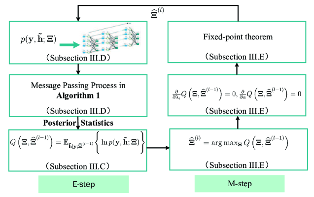
Figure 1: The block diagram of the proposed model parameter learning algorithm.

During the iteration $l$, the E-step is to derive the objective function $Q\big{(}{\boldsymbol{\Xi}},\hat{\boldsymbol{\Xi}}^{(l-1)}\big{)}$ as the expectation of $p(\mathbf{y},\tilde{\mathbf{h}};\hat{\boldsymbol{\Xi}})$ over $\tilde{\mathbf{h}}$ by setting $\boldsymbol{\Xi}$ as the estimated model parameters $\hat{\boldsymbol{\Xi}}^{(l-1)}$ in the previous iteration (Subsection III.C). Specifically, the factor graph and the GAMP algorithms are used to compute the desired posterior statistics (Subsection III.D). The M-step is to find the new estimation ${\boldsymbol{\Xi}^{(l)}}$ by maximizing $Q\big{(}{\boldsymbol{\Xi}},\hat{\boldsymbol{\Xi}}^{(l-1)}\big{)}$ (Subsection III.E). In order to clearly describe the proposed model parameters learning algorithm, we present its block diagram in Figure 1.

III-C Expectation step

In this subsection, we will derive the objective functions in (12). Since the received samples $\mathbf{y}$ are known, the objective function $Q\left(\boldsymbol{\Xi},\widehat{\boldsymbol{\Xi}}^{(l-1)}\right)$ can be expressed as

$$Q\left(\!\boldsymbol{\Xi},\!\widehat{\boldsymbol{\Xi}}^{(l-1)}\!\right)\!\! =\!\mathbb{E}_{\mathbf{\tilde{h}}|\mathbf{y};\widehat{\boldsymbol{\Xi}}^{(l-1)}}\Big{\{}\!\ln p\Big{(}\!\mathbf{y}|\mathbf{\tilde{h}};\alpha\!\Big{)}\!\Big{\}}\!+\!\mathbb{E}_{\mathbf{\tilde{h}}|\mathbf{y};\widehat{\boldsymbol{\Xi}}^{(l-1)}}\Big{\{}\ln p\Big{(}\mathbf{\tilde{h}}|\boldsymbol{\lambda};\alpha\Big{)}\Big{\}}\!\!+\!\mathbb{E}_{\mathbf{\tilde{h}}|\mathbf{y};\widehat{\boldsymbol{\Xi}}^{(l-1)}}\Big{\{}\!\ln p\Big{(}\!\boldsymbol{\lambda};\alpha\!\Big{)}\!\Big{\}},$$

$$=\sum_{m=1}^{M}\mathbb{E}_{\mathbf{\tilde{h}}|\mathbf{y};\widehat{\boldsymbol{\Xi}}^{(l-1)}}\Big{\{}\ln p\Big{(}\mathbf{y}_{m}|\mathbf{\tilde{h}}_{m};\alpha\Big{)}\Big{\}}\!+\!\sum_{m=2}^{M}\mathbb{E}_{\mathbf{\tilde{h}}|\mathbf{y};\widehat{\boldsymbol{\Xi}}^{(l-1)}}\Big{\{}\ln p\Big{(}\mathbf{\tilde{h}}_{m}|\mathbf{\tilde{h}}_{m-1},\boldsymbol{\lambda};\alpha\Big{)}\Big{\}}$$

$$\kern 10.0pt+\mathbb{E}_{\mathbf{\tilde{h}}|\mathbf{y};\widehat{\boldsymbol{\Xi}}^{(l-1)}}\Big{\{}\ln p\Big{(}\mathbf{\tilde{h}}_{1},\boldsymbol{\lambda};\alpha\Big{)}\Big{\}}\!+\!\mathbb{E}_{\mathbf{\tilde{h}}|\mathbf{y};\widehat{\boldsymbol{\Xi}}^{(l-1)}}\Big{\{}\ln p\Big{(}\boldsymbol{\lambda};\alpha\Big{)}\Big{\}}.$$ (14)

Under both the quantization and un-quantization case listed in the above section, it can be verified that the conditional PDF $p\Big{(}\mathbf{y}_{m}|\mathbf{\tilde{h}}_{m};\alpha\Big{)}$ is not related with the parameter set $\boldsymbol{\Xi}$. Furthermore, with (5), it can be checked that

$$p\Big{(}\mathbf{\tilde{h}}_{m}|\mathbf{\tilde{h}}_{m-1},\boldsymbol{\lambda};\alpha\Big{)}\sim\mathcal{CN}\Big{(}\mathbf{\tilde{h}}_{m};\alpha\mathbf{\tilde{h}}_{m-1},(1-\alpha^{2}){\boldsymbol{\Lambda}}\Big{)},$$ (15)

$$p\Big{(}\mathbf{\tilde{h}}_{1}|\boldsymbol{\lambda};\alpha\Big{)}\sim\mathcal{CN}\Big{(}\mathbf{\tilde{h}}_{1};\mathbf{0},{\boldsymbol{\Lambda}}\Big{)}.$$ (16)

Plugging (16) into (14) and taking some reorganizations, we can obtain

$$Q\!\!\left(\!\boldsymbol{\Xi},\!\widehat{\boldsymbol{\Xi}}^{(l-1)}\!\right)\!\! =\!\!\!\sum_{m=2}^{M}\!\!\Big{[}\!\frac{2\alpha}{1\!-\!\!\alpha^{2}}\mathop{\mathrm{missing}}{tr}\!\!\Big{(}\!\Re\Big{\{}\!{\boldsymbol{\Lambda}}^{-1}\mathbb{E}\Big{\{}\!\mathbf{\tilde{h}}_{m-1}\mathbf{\tilde{h}}_{m}^{H}\!\Big{|}\!\mathbf{y},\widehat{\boldsymbol{\Xi}}^{(\!l-\!1)}\!\Big{\}}\!\Big{\}}\!\Big{)}\!\!-\!\!\frac{\alpha^{2}}{1\!-\!\alpha^{2}}\mathop{\mathrm{missing}}{tr}\!\!\Big{(}\!{\boldsymbol{\Lambda}}^{-1}\mathbb{E}\!\Big{\{}\!\mathbf{\tilde{h}}_{m\!-\!1}\!\mathbf{\tilde{h}}_{m\!-\!1}^{H}\Big{|}\mathbf{y},\widehat{\boldsymbol{\Xi}}^{(l-1)}\!\Big{\}}\!\Big{)}\!\Big{]}$$

$$-\sum_{m=2}^{M}\!\frac{1}{1\!-\!\alpha^{2}}\mathop{\mathrm{missing}}{tr}\Big{(}{\boldsymbol{\Lambda}}^{-1}\mathbb{E}\Big{\{}\mathbf{\tilde{h}}_{m}\mathbf{\tilde{h}}_{m}^{H}\Big{|}\mathbf{y},\widehat{\boldsymbol{\Xi}}^{(l-1)}\Big{\}}\Big{)}-\mathop{\mathrm{missing}}{tr}\Big{(}{\boldsymbol{\Lambda}}^{-1}\mathbb{E}\Big{\{}\mathbf{\tilde{h}}_{1}\mathbf{\tilde{h}}_{1}^{H}\Big{|}\mathbf{y},\widehat{\boldsymbol{\Xi}}^{(l-1)}\Big{\}}\Big{)}$$

$$-(M-1)N\ln(1-\alpha^{2})-M\ln|\boldsymbol{\Lambda}|+\ln p(\boldsymbol{\lambda};\alpha)+C,$$ (17)

where $C$ is the items not related with $\boldsymbol{\Xi}$.

From (17), it can be found that $Q\left(\boldsymbol{\Xi},\hat{\boldsymbol{\Xi}}^{{(l-1)}}\right)$ is dependent on two posterior statistics, i.e., $\mathbb{E}\left\{\mathbf{\tilde{h}}_{m}\mathbf{\tilde{h}}_{m}^{H}|\mathbf{y},\boldsymbol{\hat{\Xi}}^{(l-1)}\right\}$, and $\mathbb{E}\left\{\mathbf{\tilde{h}}_{m-1}\mathbf{\tilde{h}}_{m}^{H}|\mathbf{y},\boldsymbol{\hat{\Xi}}^{(l-1)}\right\}$. Now, we turn to the calculations of these terms. Before calculating posterior statistics, let us define the following notations for further use

$$\mathbf{\widehat{\tilde{h}}}_{m}^{(l)} \!\stackrel{{\scriptstyle\vartriangle}}{{=}}\!\mathbb{E}\left\{\!\mathbf{\tilde{h}}_{m}|\mathbf{y},\boldsymbol{\hat{\Xi}}^{(l-1)}\!\right\},\kern 5.0pt\boldsymbol{\Theta}_{m}^{(l)}\!\stackrel{{\scriptstyle\vartriangle}}{{=}}\!\mathbb{E}\left\{\!\mathbf{\tilde{h}}_{m}\mathbf{\tilde{h}}_{m}^{H}|\mathbf{y},\boldsymbol{\hat{\Xi}}^{(l-1)}\!\right\},\kern 5.0pt\boldsymbol{\Pi}_{m-1,m}^{(l)}\!\stackrel{{\scriptstyle\vartriangle}}{{=}}\!\mathbb{E}\left\{\!\mathbf{\tilde{h}}_{m-1}\mathbf{\tilde{h}}_{m}^{H}|\mathbf{y},\boldsymbol{\hat{\Xi}}^{(l-1)}\!\right\}.$$ (18)

III-D Deriving the Posterior Statistics with GAMP

With given $\mathbf{y}$ and $\boldsymbol{\hat{\Xi}}^{(l-1)}$, our objective is to infer the posterior statistics $\widehat{\mathbf{\tilde{h}}}_{m}^{(l)}$, $\boldsymbol{\Theta}_{m}^{(l)}$, and $\boldsymbol{\Pi}_{m-1,m}^{(l)}$ under the state-space model described by the following state equation in (19) and measurement equation in (20):

$$\mathbf{\tilde{h}}_{m} =\hat{\alpha}^{(l-1)}\mathbf{\tilde{h}}_{m-1}+\sqrt{1-[\hat{\alpha}^{(l-1)}]^{2}}\boldsymbol{\upsilon}_{m},$$ (19)

$$\mathbf{y}_{m} =\mathcal{Q}\Big{\{}\underbrace{\mathbf{X}_{m}^{T}\mathbf{F}_{N}^{H}}_{\mathbf{B}_{m}}\mathbf{\tilde{h}}_{m}+\mathbf{n}_{m}\Big{\}},~{}m=1,2,\ldots,M,$$ (20)

where matrix $\mathbf{B}_{m}$ is defined in (20), and $\boldsymbol{\upsilon}_{m}\sim\mathcal{CN}(0,\boldsymbol{\Lambda}^{(l-1)})$. With the Bayes rule, the posterior joint probability density function can be computed as

$$p(\mathbf{\tilde{h}}|\mathbf{y};\widehat{\boldsymbol{\Xi}}^{(l-1)})=\frac{p\Big{(}\mathbf{y}|\mathbf{\tilde{h}};\widehat{\boldsymbol{\Xi}}^{(l-1)}\Big{)}p\Big{(}\mathbf{\tilde{h}};\widehat{\boldsymbol{\Xi}}^{(l-1)}\Big{)}}{p\Big{(}\mathbf{y};\widehat{\boldsymbol{\Xi}}^{(l-1)}\Big{)}}.$$ (21)

However, it is intractable to directly compute the desired posterior statistics, which is because of the high-dimensional integrals over the marginal distributions. To avoid this obstacle, we will resort to the factor graph and the message passing algorithms. First, the posterior joint PDF in (21) can be factorized as

$$p(\mathbf{\tilde{h}}|\mathbf{y};\widehat{\boldsymbol{\Xi}}^{(l-1)})\varpropto \prod_{m=1}^{M}\Big{\{}\prod_{p=1}^{P}f^{A}_{m,p}(\mathbf{\tilde{h}}_{k,m})\prod_{i=1}^{N}f^{B}_{m,i}(\tilde{h}_{m,i},\tilde{h}_{m-1,i})\Big{\}},$$ (22)

where $f^{A}_{m,p}(\mathbf{\tilde{h}}_{k,m})=p\Big{(}y_{m,p}|z_{m,p};\widehat{\boldsymbol{\Xi}}^{(l-1)}\Big{)},f^{B}_{m,i}(\tilde{h}_{m,i},\tilde{h}_{m-1,i})=p\Big{(}\tilde{h}_{m,i}|\tilde{h}_{m-1,i};\widehat{\boldsymbol{\Xi}}^{(l-1)}\Big{)}$,$z_{m,p}=[\mathbf{B}_{m}]_{p,:}\mathbf{\tilde{h}}_{m}$, $m=1,2,\ldots,M$, $p=1,2,\ldots,P$, and $i=1,2,\ldots,N$; The explicit expressions of $p\Big{(}y_{m,p}|z_{m,p};\widehat{\boldsymbol{\Xi}}^{(l-1)}\Big{)}$ and $p\Big{(}\tilde{h}_{m,i}|\tilde{h}_{m-1,i};\widehat{\boldsymbol{\Xi}}^{(l-1)}\Big{)}$ are presented in Appendix A.

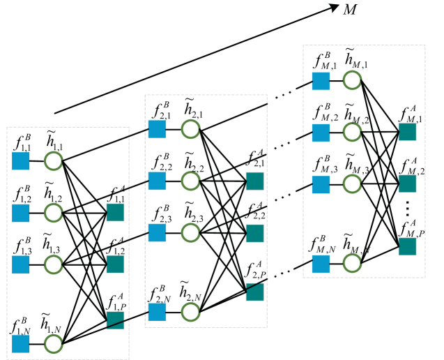
Figure 2: The Constructed Factor graph.

Then, $p(\mathbf{\tilde{h}}|\mathbf{y};\widehat{\boldsymbol{\Xi}}^{(l-1)})$ can be denoted with a factor graph, as shown in Fig. 2. Obviously, there are two kinds of function nodes, i.e., $f^{A}_{m,p}$, and $f^{B}_{m,i}$, and the variable nodes, i.e., $\tilde{h}_{m,i}$, in Fig. 2. One specific variable node $x$ connects with the function nodes $f$, whose augments contain $x$. Furthermore, for the function node $f$ and the variable node $x$, the messages from $f$ to $x$ and from $x$ to $f$ are separately defined as $\vartheta_{f\rightarrow x}(x)$ and $\vartheta_{x\rightarrow f}(x)$, whose augment is $x$. With the belief propagation (BP) theory, we can obtain

$$\vartheta_{x\rightarrow f}(x)=\prod_{f^{\prime}\in\mathcal{N}(x)/f}\vartheta_{f^{\prime}\rightarrow x}(x),\kern 20.0pt\vartheta_{f\rightarrow x}(x)=\int_{\sim x}\Big{(}f(x)\prod_{x^{\prime}\in\mathcal{N}(f)/x}\vartheta_{x^{\prime}\rightarrow f}(x^{\prime}))\Big{)},$$ (23)

where the set $\mathcal{N}(x)$ collects all the neighbouring nods of the given node $x$ in one factor graph, and $\sim x$ possesses the same meaning with the same notation in [32].

However, due to the presence of the cycles, BP can not be directly applied for Fig. 2. Nonetheless, the message scheduling and general approximate message propagation (GAMP) algorithms can be adopted to effectively approximate the posterior distribution within the given allowable iterations. Specially, the message scheduling can be divided into three steps, i.e., the forward message passing, the message exchanging, and the backward message passing. For clarity, we list the corresponding messages in Table I.

TABLE I: Different messages between nodes

Notations	Definitions	Values
$\vartheta_{f^{A}_{m,p}\to\tilde{h}_{m,i}}(\tilde{h}_{m,i})$	belief from $f^{A}_{m,p}$ to $\tilde{h}_{m,i}$	$\mathcal{CN}\left(\tilde{h}_{m,i};\mu_{f^{A}_{m,p}\to\tilde{h}_{m,i}},\nu_{f^{A}_{m,p}\to\tilde{h}_{m,i}}\right)$
$\vartheta_{f^{B}_{m,i}\to\tilde{h}_{m,i}}(\tilde{h}_{m,i})$	belief from $f^{B}_{m,i}$ to $\tilde{h}_{m,i}$	$\mathcal{CN}\left(\tilde{h}_{m,i};\mu_{f^{B}_{m,i}\to\tilde{h}_{m,i}},\nu_{f^{B}_{m,i}\to\tilde{h}_{m,i}}\right)$
$\vartheta_{f^{B}_{m+1,i}\to\tilde{h}_{m,i}}(\tilde{h}_{m,i})$	belief from $f^{B}_{m+1,i}$ to $\tilde{h}_{m,i}$	$\mathcal{CN}\left(\tilde{h}_{m,i};\mu_{f^{B}_{m+1,i}\to\tilde{h}_{m,i}},\nu_{f^{B}_{m+1,i}\to\tilde{h}_{m,i}}\right)$
$\prod\limits_{p=1}^{P}\vartheta_{f^{A}_{m,p}\to\tilde{h}_{m,i}}(\tilde{h}_{m,i})$	the sum product belief to $\tilde{h}_{m,i}$	$\mathcal{CN}\left(\tilde{h}_{m,i};\bar{\mu}_{f^{A}_{m,:}\to\tilde{h}_{m,i}},\bar{\nu}_{f^{A}_{m,:}\to\tilde{h}_{m,i}}\right)$

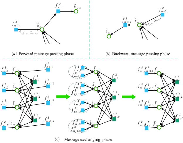
Figure 3: (a)The sub-factor-graph for the forward message passing into the mth time blockp. (b)The sub-factor-graph for the message exchanging within the $m$th time block. (c)The sub-factor-graph for the backward message passing into the mth time blockp.

III-D1 The belief updating for the forward message passing into the $\boldsymbol{m}$-th time block

Within this step, the beliefs are passed from the variable nodes $\tilde{h}_{m-1,i}$ into the $m$th time block through the function nodes $f^{B}_{m,i}$, and the believes $\vartheta_{f_{m,i}^{B}\to\tilde{h}_{m,i}}$ will be updated in the sub-graph Fig. 3(a) [33]. Thus, for $2\leq m\leq M$, with (22), (23) and Table. I, we can obtain

$$\vartheta_{f_{m,i}^{B}\to\tilde{h}_{m,i}}\!\propto\!\int_{\tilde{h}_{m-1,i}}\!\!f_{m,i}^{B}\vartheta_{\tilde{h}_{m-1,i}\to f_{m,i}^{B}}d\tilde{h}_{m-1,i}\!=\!\int_{\tilde{h}_{m-1,i}}f_{m,i}^{B}\vartheta_{f_{m-1,i}^{B}\to\tilde{h}_{m-1,i}}\prod_{P=1}^{P}\vartheta_{f_{m-1,p}^{A}\to\tilde{h}_{m-1,i}}d\tilde{h}_{m-1,i}$$

$$\propto\int_{\tilde{h}_{m-1,i}}\mathcal{CN}\left(\tilde{h}_{m-1,i};\mu_{f_{m-1,i}^{B}\to\tilde{h}_{m-1,i}},\nu_{f_{m-1,i}^{B}\to\tilde{h}_{m-1,i}}\right)\mathcal{CN}\left(\tilde{h}_{m-1,i};{\bar{\mu}}_{f_{m-1,:}^{A}\to\tilde{h}_{m-1,i}},\bar{\nu}_{f_{m-1,:}^{A}\to\tilde{h}_{m-1,i}}\right)$$

$$\times\mathcal{CN}\left(\tilde{h}_{m,i};\hat{\alpha}^{(l-1)}\tilde{h}_{m-1,i},\Big{(}1-\Big{[}\hat{\alpha}^{(l-1)}\Big{]}^{2}\Big{)}\hat{\lambda}_{i}^{(l-1)}\right)d\tilde{h}_{m-1,i}$$

$$=\mathcal{CN}\left(\tilde{h}_{m,i};\mu_{f_{m,i}^{B}\to\tilde{h}_{m,i}},\nu_{f_{m,i}^{B}\to\tilde{h}_{m,i}}\right),$$ (24)

where

$$\mu_{f_{m,i}^{B}\to\tilde{h}_{m,i}}= \hat{\alpha}^{(l-1)}\left(\frac{\bar{\mu}_{f_{m-1,:}^{A}\to\tilde{h}_{m-1,i}}}{\bar{\nu}_{f_{m-1,:}^{A}\to\tilde{h}_{m-1,i}}}+\frac{\mu_{f_{m-1,i}^{B}\to\tilde{h}_{m-1,i}}}{\nu_{f_{m-1,i}^{B}\to\tilde{h}_{m-1,i}}}\right)\frac{\bar{\nu}_{f_{m-1,:}^{A}\to\tilde{h}_{m-1,i}}\nu_{f_{m-1,i}^{B}\to\tilde{h}_{m-1,i}}}{\bar{\nu}_{f_{m-1,i}^{A}\to\tilde{h}_{m-1,i}}+\nu_{f_{m-1,i}^{B}\to\tilde{h}_{m-1,i}}},$$ (25)

$$\nu_{f_{m,i}^{B}\to\tilde{h}_{m,i}}= \left[\hat{\alpha}^{(l-1)}\right]^{2}\frac{\bar{\nu}_{f_{m-1,:}^{A}\to\tilde{h}_{m-1,i}}\nu_{f_{m-1,i}^{B}\to\tilde{h}_{m-1,i}}}{\bar{\nu}_{f_{m-1,:}^{A}\to\tilde{h}_{m-1,i}}+\nu_{f_{m-1,i}^{B}\to\tilde{h}_{m-1,i}}}+\left(1-\left[\hat{\alpha}^{(l-1)}\right]^{2}\right)\hat{\lambda}_{i}^{(l-1)},$$ (26)

and the property $\prod\limits_{n}\mathcal{CN}(r;\mu_{n},\nu_{n})\propto\mathcal{CN}\left(r;\frac{\sum\limits_{n}\mu_{n}/\nu_{n}}{\sum\limits_{n}1/\nu_{n}},\frac{1}{\sum\limits_{n}1/\nu_{n}}\right)$ is utilized in the above derivation. Specially, at $M=1$, we have $\vartheta_{f_{1,i}^{B}\to\tilde{h}_{1,i}}=\mathcal{CN}(\tilde{h}_{1,i};\mu_{f_{1,i}^{B}\to\tilde{h}_{1,i}},\nu_{f_{1,i}^{B}\to\tilde{h}_{1,i}})$, $\mu_{f_{1,i}^{B}\to\tilde{h}_{1,i}}=0$, and $\nu_{f_{1,i}^{B}\to\tilde{h}_{1,i}}=\hat{\lambda}_{1}^{(l-1)}$.

III-D2 The belief updating for the message exchanging within the $\boldsymbol{m}$-th time block

In this step, we will obtain the estimation of $\tilde{h}_{m,i}$ through exchanging information within the $m$th time block, where $\mathbf{y}_{m}$, and $\vartheta_{f^{B}_{m+1,i}\to\tilde{h}_{m,i}}$, $\vartheta_{f^{B}_{m,i}\to\tilde{h}_{m,i}}$ are utilized. With the left sub-figure of Fig. 3(c) and Table. I, the sum product belief from both $f^{B}_{m+1,i}$ and $f^{B}_{m,i}$ to $\tilde{h}_{m,i}$ can be written as

$$\vartheta_{\{f^{B}_{m+1,i},f^{B}_{m,i}\}\to\tilde{h}_{m,i}}\propto \mathcal{CN}\left(\tilde{h}_{m,i};\mu_{f^{B}_{m+1,i}\to\tilde{h}_{m,i}},\nu_{f^{B}_{m+1,i}\to\tilde{h}_{m,i}}\right)\mathcal{CN}\left(\tilde{h}_{m,i};\mu_{f^{B}_{m,i}\to\tilde{h}_{m,i}},\nu_{f^{B}_{m,i}\to\tilde{h}_{m,i}}\right)$$

$$\propto \mathcal{CN}\left(\tilde{h}_{m,i};\mu_{\{f^{B}_{m+1,i},f^{B}_{m,i}\}\to\tilde{h}_{m,i}},\nu_{\{f^{B}_{m+1,i},f^{B}_{m,i}\}\to\tilde{h}_{m,i}}\right),$$ (27)

$$\text{where}~{}~{}~{}~{}~{}~{}~{}~{}~{}~{}~{}\nu_{\{f^{B}_{m+1,i},f^{B}_{m,i}\}\to\tilde{h}_{m,i}}= \frac{\nu_{f_{m,i}^{B}\to\tilde{h}_{m,i}}\nu_{f_{m+1,i}^{B}\to\tilde{h}_{m,i}}}{\nu_{f_{m,i}^{B}\to\tilde{h}_{m,i}}+\nu_{f_{m+1,i}^{B}\to\tilde{h}_{m,i}}},$$ (28)

$$\mu_{\{f^{B}_{m+1,i},f^{B}_{m,i}\}\to\tilde{h}_{m,i}}= \nu_{\{f^{B}_{m+1,i},f^{B}_{m,i}\}\to\tilde{h}_{m,i}}\left(\frac{\mu_{f_{m,i}^{B}\to\tilde{h}_{m,i}}}{\nu_{f_{m,i}^{B}\to\tilde{h}_{m,i}}}+\frac{\mu_{f_{m+1,i}^{B}\to\tilde{h}_{m,i}}}{\nu_{f_{m+1,i}^{B}\to\tilde{h}_{m,i}}}\right).~{}~{}~{}~{}~{}$$ (29)

With this observation, we can treat the nodes $\{f^{B}_{m+1,i},f^{B}_{m,i}\}$ together, and obtain Fig. 3(c), which is the same to the factor graph for the GAMP [34]. In fact, if we only consider the right sub-figure of Fig. 3(c), the MMSE estimation of $\tilde{h}_{m,i}$ can be solved through the GAMP with respect to the observation model

$$\mathbf{y}_{m}=\mathcal{Q}\{\mathbf{z}_{m}+\mathbf{n}_{m}\},$$ (30)

where $\mathbf{z}_{m}=[z_{m,1},z_{m,2},\ldots,z_{m,P}]^{T}$, and the prior knowledge about $\tilde{h}_{m,i}$ can be expressed as

$$p(\tilde{h}_{m,i})=\mathcal{CN}\left(\tilde{h}_{m,i};\mu_{\{f^{B}_{m+1,i},f^{B}_{m,i}\}\to\tilde{h}_{m,i}},\nu_{\{f^{B}_{m+1,i},f^{B}_{m,i}\}\to\tilde{h}_{m,i}}\right).$$ (31)

III-D3 The backward message passing into $\boldsymbol{m}$-th time block.

Within this step, the believes about variable node $\tilde{h}_{m+1,i}$ will be passed into the $m$th time block in the backward manner within Fig. 3(b), where the related belief is $\vartheta_{f_{m+1,i}^{B}\to\tilde{h}_{m,i}}$, respectively. Following the similar methods, we can calculate $\vartheta_{f_{m+1,i}^{B}\to\tilde{h}_{m,i}}$ as

$$\vartheta_{f_{m+1,i}^{B}\to\tilde{h}_{m,i}}$$

$$\propto\int_{\tilde{h}_{m+1,i}}f_{m+1,i}^{B}\vartheta_{\tilde{h}_{m+1,i}\to f_{m+1,i}^{B}}d\tilde{h}_{m+1,i}=\int_{\tilde{h}_{m+1,i}}f_{m+1,i}^{B}\vartheta_{f_{m+2,i}^{B}\to\tilde{h}_{m+1,i}}\prod_{P=1}^{P}\vartheta_{f_{m+1,p}^{A}\to\tilde{h}_{m+1,i}}d\tilde{h}_{m+1,i}$$

$$\propto\int_{\tilde{h}_{m+1,i}}\mathcal{CN}\left(\tilde{h}_{m+1,i};\mu_{f_{m+2,i}^{B}\to\tilde{h}_{m+1,i}},\nu_{f_{m+2,i}^{B}\to\tilde{h}_{m+1,i}}\right)\mathcal{CN}\left(\tilde{h}_{m+1,i};{\bar{\mu}}_{f_{m+1,:}^{A}\to\tilde{h}_{m+1,i}},\bar{\nu}_{f_{m+1,:}^{A}\to\tilde{h}_{m+1,i}}\right)$$

$$~{}~{}\times\mathcal{CN}\left(\tilde{h}_{m+1,i};\hat{\alpha}^{(l-1)}\tilde{h}_{m,i},\Big{(}1-\Big{[}\hat{\alpha}^{(l-1)}\Big{]}^{2}\Big{)}\hat{\lambda}_{i}^{(l-1)}\right)d\tilde{h}_{m+1,i}$$

$$=\mathcal{CN}\left(\tilde{h}_{m,i};\mu_{f_{m+1,i}^{B}\to\tilde{h}_{m,i}},\nu_{f_{m+1,i}^{B}\to\tilde{h}_{m,i}}\right),$$ (32)

where

$$\mu_{f_{m+1,i}^{B}\to\tilde{h}_{m,i}}= \frac{1}{\hat{\alpha}^{(l-1)}}\left(\frac{\bar{\mu}_{f_{m+1,:}^{A}\to\tilde{h}_{m+1,i}}}{\bar{\nu}_{f_{m+1,:}^{A}\to\tilde{h}_{m+1,i}}}+\frac{\mu_{f_{m+2,i}^{B}\to\tilde{h}_{m+1,i}}}{\nu_{f_{m+2,i}^{B}\to\tilde{h}_{m+1,i}}}\right)\frac{\bar{\nu}_{f_{m+1,:}^{A}\to\tilde{h}_{m+1,i}}\nu_{f_{m+2,i}^{B}\to\tilde{h}_{m+1,i}}}{\bar{\nu}_{f_{m+1,i}^{A}\to\tilde{h}_{m+1,i}}+\nu_{f_{m+2,i}^{B}\to\tilde{h}_{m+1,i}}},$$ (33)

$$\nu_{f_{m+1,i}^{B}\to\tilde{h}_{m,i}}= \frac{1}{\left[\hat{\alpha}^{(l-1)}\right]^{2}}\left(\frac{\bar{\nu}_{f_{m+1,:}^{A}\to\tilde{h}_{m+1,i}}\nu_{f_{m+2,i}^{B}\to\tilde{h}_{m+1,i}}}{\bar{\nu}_{f_{m+1,:}^{A}\to\tilde{h}_{m+1,i}}+\nu_{f_{m+2,i}^{B}\to\tilde{h}_{m+1,i}}}+\left(1-\left[\hat{\alpha}^{(l-1)}\right]^{2}\right)\hat{\lambda}_{i}^{(l-1)}\right),$$ (34)

$m=1,2,\ldots,M-1$. Furthermore, we can set $\vartheta_{f_{M+1,i}^{B}\to\tilde{h}_{M,i}}=\mathcal{CN}(\tilde{h}_{M,i};0,+\infty)$.

Algorithm 1 The Message Passing Process for the expectation step of the $l$th EM iteration

0:  : Matrix $\mathbf{B}_{m}$, scalar estimation functions $g_{s}$ and $g_{\tilde{h}}$,and damping constants $\theta_{s}$,$\theta_{\tilde{h}}\in(0,1]$.

1:  k=0, Initialize $\boldsymbol{\nu}_{{\tilde{h}},m}^{(k=0)}>\text{diag}\Big{(}\boldsymbol{\Theta}_{m}^{(l-1)}-\widehat{\mathbf{\tilde{h}}}_{m}^{(l-1)}\Big{(}\widehat{\mathbf{\tilde{h}}}_{m}^{(l-1)}\Big{)}^{H}\Big{)},\mathbf{\tilde{h}}_{m}^{(k=0)}=\widehat{\mathbf{\tilde{h}}}_{m}^{(l-1)}$, $\mathbf{s}_{m}^{(k=0)}=\widehat{\mathbf{s}}_{m}^{(l-1)}$.

2:  repeat

3:     Implement the forward message passing into the $m$th time block, $i=1$.

4:     repeat

5:        $k=k+1$

6:        $i=i+1$, $m=1$, $\mu_{f_{1,i}^{B}\to\tilde{h}_{1,i}}=0$, $\nu_{f_{1,i}^{B}\to\tilde{h}_{1,i}}=\hat{\lambda}_{1}^{(l-1)}$.

7:        repeat

8:           $m=m+1$.

9:           $\mu_{f_{m,i}^{B}\to\tilde{h}_{m,i}}=\hat{\alpha}^{(l-1)}\left(\frac{\bar{\mu}_{f_{m-1,:}^{A}\to\tilde{h}_{m-1,i}}}{\bar{\nu}_{f_{m-1,:}^{A}\to\tilde{h}_{m-1,i}}}+\frac{\mu_{f_{m-1,i}^{B}\to\tilde{h}_{m-1,i}}}{\nu_{f_{m-1,i}^{B}\to\tilde{h}_{m-1,i}}}\right)\frac{\bar{\nu}_{f_{m-1,:}^{A}\to\tilde{h}_{m-1,i}}\nu_{f_{m-1,i}^{B}\to\tilde{h}_{m-1,i}}}{\bar{\nu}_{f_{m-1,i}^{A}\to\tilde{h}_{m-1,i}}+\nu_{f_{m-1,i}^{B}\to\tilde{h}_{m-1,i}}}$.

10:           $\nu_{f_{m,i}^{B}\to\tilde{h}_{m,i}}=\left[\hat{\alpha}^{(l-1)}\right]^{2}\frac{\bar{\nu}_{f_{m-1,:}^{A}\to\tilde{h}_{m-1,i}}\nu_{f_{m-1,i}^{B}\to\tilde{h}_{m-1,i}}}{\bar{\nu}_{f_{m-1,:}^{A}\to\tilde{h}_{m-1,i}}+\nu_{f_{m-1,i}^{B}\to\tilde{h}_{m-1,i}}}+\left(1-\left[\hat{\alpha}^{(l-1)}\right]^{2}\right)\hat{\lambda}_{i}^{(l-1)}$

11:        until $m=M$

12:     until $i=N$

13:     Implement the message exchanging within the $m$th time block, $m=1$

14:     repeat

15:        $\mathbf{S}=\mathbf{B}_{m}.\mathbf{B}_{m}$(component-wise magnitude squared)

16:        1./$\boldsymbol{\nu}_{p,m}^{(k)}=\mathbf{S}\boldsymbol{\nu}_{{\tilde{h}},m}^{(k)}$,$\mathbf{p}_{m}^{(k)}=\mathbf{s}_{m}^{(k-1)}+\boldsymbol{\nu}_{p,m}^{(k)}.\mathbf{B}_{m}\mathbf{\tilde{h}}_{m}^{(k)}$.

17:        $\boldsymbol{\nu}_{s,m}^{(k)}=\boldsymbol{\nu}_{p,m}^{(k)}.g_{s}^{\prime}\left(\mathbf{p}_{m}^{{(k)}},\boldsymbol{\nu}_{p,m}^{(k)}\right)$, $\mathbf{s}_{m}^{(k)}=(1-\theta_{s})\mathbf{s}_{m}^{(k-1)}+\theta_{s}g_{s}\left(\mathbf{p}_{m}^{(k)},\boldsymbol{\nu}_{p,m}^{(k)}\right)$.

18:        1./${\boldsymbol{\nu}}_{r,m}^{(k)}=\mathbf{S}_{m}^{T}\boldsymbol{\nu}_{s,m}^{(k)}$,$\mathbf{r}_{m}^{(k)}=\mathbf{\tilde{h}}_{m}^{(k)}-\boldsymbol{\nu}_{r,m}^{(k)}.\mathbf{B}_{m}^{H}\mathbf{s}_{m}^{(k)}$.

19:        $\boldsymbol{\tau}_{{\tilde{h}},m}^{(k+1)}=\boldsymbol{\nu}_{r,m}^{(k)}.g_{{\tilde{h}},m}^{\prime}(\mathbf{r}_{m}^{(k)},\boldsymbol{\nu}_{r,m}^{(k)})$,$\mathbf{\tilde{h}}_{m}^{(k+1)}=(1-\theta_{\tilde{h}})\mathbf{\tilde{h}}_{m}^{{k}}+\theta_{\tilde{h}}g_{{\tilde{h}},m}(\mathbf{r}_{m}^{(k)},\boldsymbol{\nu}_{r,m}^{(k)})$.

20:        $m=m+1$.

21:     until $m=M$

22:     for $i=1$ to $i=N$, $\bar{\mu}_{f^{A}_{m,:}\to\tilde{h}_{m,i}}=[\mathbf{r}_{m}^{(k)}]_{i}$, $\bar{\nu}_{f^{A}_{m,:}\to\tilde{h}_{m,i}}=[\boldsymbol{\nu}_{r,m}^{(k)}]_{i}$.

23:     Implement the backward message passing into the $m$th time block, $i=1$.

24:     repeat

25:        $i=i+1$, $m=M$, $\mu_{f_{M+1,i}^{B}\to\tilde{h}_{M,i}}=0$, $\nu_{f_{M+1,i}^{B}\to\tilde{h}_{M,i}}=\mathcal{CN}(\tilde{h}_{M,i};0,+\infty)=\infty$.

26:        repeat

27:           $m=m-1$.

28:           $\mu_{f_{m+1,i}^{B}\to\tilde{h}_{m,i}}=\frac{1}{\hat{\alpha}^{(l-1)}}\left(\frac{\bar{\mu}_{f_{m+1,:}^{A}\to\tilde{h}_{m+1,i}}}{\bar{\nu}_{f_{m+1,:}^{A}\to\tilde{h}_{m+1,i}}}+\frac{\mu_{f_{m+2,i}^{B}\to\tilde{h}_{m+1,i}}}{\nu_{f_{m+2,i}^{B}\to\tilde{h}_{m+1,i}}}\right)\frac{\bar{\nu}_{f_{m+1,:}^{A}\to\tilde{h}_{m+1,i}}\nu_{f_{m+2,i}^{B}\to\tilde{h}_{m+1,i}}}{\bar{\nu}_{f_{m+1,i}^{A}\to\tilde{h}_{m+1,i}}+\nu_{f_{m+2,i}^{B}\to\tilde{h}_{m+1,i}}}$,

29:           $\nu_{f_{m+1,i}^{B}\to\tilde{h}_{m,i}}=\frac{1}{\left[\hat{\alpha}^{(l-1)}\right]^{2}}\left(\frac{\bar{\nu}_{f_{m+1,:}^{A}\to\tilde{h}_{m+1,i}}\nu_{f_{m+2,i}^{B}\to\tilde{h}_{m+1,i}}}{\bar{\nu}_{f_{m+1,:}^{A}\to\tilde{h}_{m+1,i}}+\nu_{f_{m+2,i}^{B}\to\tilde{h}_{m+1,i}}}+\left(1-\left[\hat{\alpha}^{(l-1)}\right]^{2}\right)\hat{\lambda}_{i}^{(l-1)}\right)$,

30:        until $m=1$

31:     until $i=N$

32:  until $k=K_{max}$

33:  Output the estimation results of the $l$th EM iteration, i.e., $\widehat{\mathbf{s}}_{m}^{(l)}={\mathbf{s}}_{m}^{(K_{max})}$, $\widehat{\mathbf{\tilde{h}}}_{m}^{(l)}={\mathbf{\tilde{h}}}_{m}^{(K_{max}+1)}$, $\boldsymbol{\Theta}_{m}^{(l)}=\text{Diag}\Big{(}\boldsymbol{\tau}_{{\tilde{h}},m}^{(K_{max}+1)}\Big{)}+\widehat{\mathbf{\tilde{h}}}_{m}^{(l)}\Big{(}\widehat{\mathbf{\tilde{h}}}_{m}^{(l)}\Big{)}^{H}$, $i=1,2,\ldots,N$, $M=1,2,\ldots,M$.

Taking the above three message updating phases into consideration, we can listed the detailed steps for the expectation step of the $l$th EM iteration in Algorithm 1. In this algorithm, the notations $\mathbf{a}.\mathbf{b}$ and $\mathbf{a}./\mathbf{b}$ denote the component-wise multiplication and division, respectively. Furthermore, the input scalar estimation function $g_{s}\left(\mathbf{p},\boldsymbol{\nu}_{\mathbf{p}}\right)$ and that for the output $g_{\tilde{h}}(\mathbf{r},\boldsymbol{\nu}_{\mathbf{r}})$ can be separately defined as

$$\left[g_{s}\left(\mathbf{p},\boldsymbol{\nu}_{p}\right)\right]_{n}= p_{n}-\nu_{p,n}\frac{\int z_{m,n}p({y_{m,n}|z_{m,n}})\mathcal{CN}({z}_{m,n};\frac{p_{n}}{\nu_{p,n}},\frac{1}{\nu_{p,n}})d{z}_{m,n}}{\int p({y_{m,n}|z_{m,n}})\mathcal{CN}({z}_{m,n};\frac{p_{n}}{\nu_{p,n}},\frac{1}{\nu_{p,n}})d{z}_{m,n}},$$ (35)

$$\left[g_{{\tilde{h}}}\left(\mathbf{r},\boldsymbol{\nu}_{\mathbf{r}}\right)\right]_{i}= \frac{\int{\tilde{h}}_{m,i}p({\tilde{h}}_{m,i})\mathcal{CN}({\tilde{h}}_{m,i};r_{i},\nu_{{r},i})d{\tilde{h}}_{m,i}}{\int p({\tilde{h}}_{m,i})\mathcal{CN}({\tilde{h}}_{m,i};r_{i},\nu_{{r},i})d{\tilde{h}}_{m,i}},$$ (36)

where $\mathbf{r}=[r_{1},r_{2},\ldots,r_{N}]^{T}$, $\boldsymbol{\nu}_{r}=[\nu_{r,1},\nu_{r,2},\ldots,\nu_{r,N}]^{T}$, $\mathbf{p}=[p_{1},p_{2},\ldots,p_{P}]^{T}$, and $\boldsymbol{\nu}_{p}=[\nu_{p,1},\nu_{p,2},\ldots,\nu_{p,P}]^{T}$. In Appendix B, we derive $g_{s}\left(\mathbf{p},\boldsymbol{\nu}_{\mathbf{p}}\right)$, $g_{\tilde{h}}(\mathbf{r},\boldsymbol{\nu}_{\mathbf{r}})$ and their corresponding partial derivatives. For clarity, we show them in Table. II, where the explicit expressions of $\Delta^{\Re}_{m,n}$, $\Delta^{\Im}_{m,n}$, $\nabla^{\Re}_{m,n}$, $\nabla^{\Im}_{m,n}$, $\Xi^{\Re}_{m,n}$, and $\Xi^{\Im}_{m,n}$ are presented in Appendix B.

TABLE II: The values of $g_{s}\left(\mathbf{p},\boldsymbol{\nu}_{\mathbf{p}}\right)$, $g_{\tilde{h}}(\mathbf{r},\boldsymbol{\nu}_{\mathbf{r}})$ and their partial derivatives under different quantization cases

The quantization Cases	The values of $g_{s}\left(\mathbf{p}\!,\!\boldsymbol{\nu}_{\mathbf{p}}\right)$, $g_{\tilde{h}}(\mathbf{r},\!\boldsymbol{\nu}_{\mathbf{r}})$ and their partial derivatives
No quantization	$\left[g_{\mathbf{s}}\left(\mathbf{p},\boldsymbol{\nu}_{\mathbf{p}}\right)\right]_{n}=\frac{p_{n}-\nu_{p,n}{y_{m,n}}}{1+\nu_{p,n}{\sigma_{n}^{2}}}$, $\left[g_{\mathbf{s}}^{\prime}\left(\mathbf{p},\boldsymbol{\nu}_{\mathbf{p}}\right)\right]_{n}=\frac{1}{1+\nu_{p,n}{\sigma_{n}^{2}}}$.
Normal Quantization	$\left[g_{\mathbf{s}}\left(\mathbf{p},\boldsymbol{\nu}_{\mathbf{p}}\right)\right]_{n}\!=\!\!\frac{1}{2}\frac{\Delta^{\Re}_{m,n}}{\nabla^{\Re}_{m,n}}+\frac{1}{2}\jmath\frac{\Delta^{\Im}_{m,n}}{\nabla^{\Im}_{m,n}}$,
	$[g_{s}^{\prime}\left(\mathbf{p},\boldsymbol{\nu}_{\mathbf{p}}\right)]_{n}\!=\!\frac{1}{4\nu_{p,n}\sqrt{\frac{1}{2}(\sigma_{n}^{2}\!+\!\frac{1}{\nu_{p,n}})}}\left\{\frac{\Xi^{\Re}_{m,n}}{\nabla^{\Re}_{m,n}}\!+\!\frac{\Xi^{\Im}_{m,n}}{\nabla^{\Im}_{m,n}}\right\}\!+\!\frac{1}{\nu_{p,n}}|\left[\!g_{s}\left(\!\mathbf{p},\boldsymbol{\nu}_{p}\!\right)\!\right]_{n}|^{2}$.
PDQ case	$\left[g_{\mathbf{s}}\left(\mathbf{p},\boldsymbol{\nu}_{\mathbf{p}}\right)\right]_{n}=\frac{(1-\rho)p_{n}-\nu_{p,n}y_{m,n}}{(1-\rho)+\nu_{p,n}[(1-\rho)\sigma_{n}^{2}+\rho]}$, $\left[g_{\mathbf{s}}^{\prime}\left(\mathbf{p},\boldsymbol{\nu}_{\mathbf{p}}\right)\right]_{n}=\frac{1-\rho}{(1-\rho)+\nu_{p,n}[(1-\rho)\sigma_{n}^{2}+\rho]}$.
All the cases	$\left[g_{{\tilde{h}}}\left(\mathbf{r},\boldsymbol{\nu}_{\mathbf{r}}\right)\right]_{i}=\frac{\mu_{\{f^{B}_{m+1,i},f^{B}_{m,i}\}\to\tilde{h}_{m,i}}\nu_{{r},i}+r_{i}\nu_{\{f^{B}_{m+1,i},f^{B}_{m,i}\}\to\tilde{h}_{m,i}}}{\nu_{\{f^{B}_{m+1,i},f^{B}_{m,i}\}\to\tilde{h}_{m,i}}+\nu_{{r},i}}$,
	$\left[g_{{\tilde{h}}}^{\prime}\left(\mathbf{r},\boldsymbol{\nu}_{\mathbf{r}}\right)\right]_{i}=\frac{\nu_{\{f^{B}_{m+1,i},f^{B}_{m,i}\}\to\tilde{h}_{m,i}}}{\nu_{\{f^{B}_{m+1,i},f^{B}_{m,i}\}\to\tilde{h}_{m,i}}+\nu_{{r},i}}$.

III-E Maximization Step

In this step, we will derive $\boldsymbol{\hat{\Xi}}^{(l)}$ through maximizing $Q\big{(}{\boldsymbol{\Xi}},\hat{\boldsymbol{\Xi}}^{(l-1)}\big{)}$ as

$$\boldsymbol{\hat{\Xi}}^{(l)}=\arg\max_{{\boldsymbol{\Xi}}}\left\{Q\big{(}{\boldsymbol{\Xi}},\hat{\boldsymbol{\Xi}}^{(l-1)}\big{)}\right\}.$$ (P1)

Taking the derivative of (17) with respect to $\lambda_{i}$ and $\alpha$, we can obtain

$$\frac{\partial}{\partial\lambda_{i}}Q\left(\boldsymbol{\Xi},\widehat{\boldsymbol{\Xi}}^{(l-1)}\right)= \sum_{m=2}^{M}\Big{[}-\frac{2\alpha}{1-\alpha^{2}}\frac{1}{\lambda_{i}^{2}}\Re\Big{\{}\Big{[}\boldsymbol{\Pi}_{m-1,m}^{(l)}\Big{]}_{i,i}\Big{\}}+\frac{\alpha^{2}}{1-\alpha^{2}}\frac{1}{\lambda_{i}^{2}}\Big{[}\boldsymbol{\Theta}_{m-1}^{(l)}\Big{]}_{i,i}\Big{]}$$

$$+\sum_{m=2}^{M}\frac{1}{1-\alpha^{2}}\frac{1}{\lambda_{i}^{2}}\Big{[}\boldsymbol{\Theta}_{m}^{(l)}\Big{]}_{i,i}+\frac{1}{\lambda_{i}^{2}}\Big{[}\boldsymbol{\Theta}_{1}^{(l)}\Big{]}_{i,i}-M\frac{1}{\lambda_{i}}+\frac{\partial\ln p(\boldsymbol{\lambda})}{\partial\lambda_{i}},$$ (37)

$$\frac{\partial}{\partial\alpha}Q\left(\boldsymbol{\Xi},\widehat{\boldsymbol{\Xi}}^{(l-1)}\right)= \sum_{m=2}^{M}\Big{[}\frac{2+2\alpha^{2}}{(1-\alpha^{2})^{2}}\mathop{\mathrm{missing}}{tr}\Big{(}\Re\Big{\{}{\boldsymbol{\Lambda}}^{-1}\boldsymbol{\Pi}_{m-1,m}^{(l)}\Big{\}}\Big{)}-\frac{2\alpha}{(1-\alpha^{2})^{2}}\mathop{\mathrm{missing}}{tr}\Big{(}{\boldsymbol{\Lambda}}^{-1}\boldsymbol{\Theta}_{m-1}^{(l)}\Big{)}\Big{]}$$

$$-\sum_{m=2}^{M}\frac{2\alpha}{(1-\alpha^{2})^{2}}\mathop{\mathrm{missing}}{tr}\Big{(}{\boldsymbol{\Lambda}}^{-1}\boldsymbol{\Theta}_{m}^{(l)}\Big{)}+(M-1)N\frac{2\alpha}{1-\alpha^{2}}.$$ (38)

Theoretically, under the sparse Bayesian learning framework, the non-informative prior is used for $p(\boldsymbol{\lambda})$. Hence, we can ignore the effect of $p(\boldsymbol{\lambda})$ in the maximization step. Correspondingly, with fixed $\alpha$, by setting the derivatives to zero, the parameter ${\lambda}_{i}^{(l)}$ can be written as

$$\lambda_{i}=\frac{1}{M}\Big{\{}\sum_{m=2}^{M}\Big{[}\!-\!\frac{2\alpha}{1-\!\!\alpha^{2}}\Re\big{\{}\big{[}\boldsymbol{\Pi}_{m-1,m}^{(l)}\big{]}_{i,i}\big{\}}\!+\!\frac{\alpha^{2}}{1-\alpha^{2}}\big{[}\boldsymbol{\Theta}_{m-1}^{(l)}\big{]}_{i,i}\!+\!\frac{1}{1-\alpha^{2}}\big{[}\!\boldsymbol{\Theta}_{m}^{(l)}\big{]}_{i,i}\Big{]}\!\!+\!\!\big{[}\boldsymbol{\Theta}_{1}^{(l)}\big{]}_{i,i}\!\Big{\}}.$$ (39)

On the other hand, with given $\lambda_{i}$, $\alpha$ can be achieved through solving the following third-order equation as

$$(M-1)N\alpha^{3}-\sum_{m=2}^{M}\Big{(}\mathop{\mathrm{missing}}{tr}\Big{(}\Re\Big{\{}{\boldsymbol{\Lambda}}^{-1}\boldsymbol{\Pi}_{m-1,m}^{(l)}\Big{\}}\Big{)}\Big{)}\alpha^{2}-\sum_{m=2}^{M}\Big{(}\mathop{\mathrm{missing}}{tr}\Big{(}\Re\Big{\{}{\boldsymbol{\Lambda}}^{-1}\boldsymbol{\Pi}_{m-1,m}^{(l)}\Big{\}}\Big{)}\Big{)}$$

$$+\left(\sum_{m=2}^{M}\Big{(}\mathop{\mathrm{missing}}{tr}\Big{(}{\boldsymbol{\Lambda}}^{-1}\boldsymbol{\Theta}_{m-1}^{(l)}\Big{)}\Big{)}+\sum_{m=2}^{M}\Big{(}\mathop{\mathrm{missing}}{tr}\Big{(}{\boldsymbol{\Lambda}}^{-1}\boldsymbol{\Theta}_{m}^{(l)}\Big{)}\Big{)}-(M-1)N\right)\alpha=0.$$ (40)

With (39) and (40), we can utilize the fixed-point theorem to obtain $\widehat{\lambda}_{i}^{(l)}$ and $\widehat{\alpha}^{(l)}$. Notice that the term $\boldsymbol{\Pi}_{m-1,m}^{(l)}$ can be written as

$$\boldsymbol{\Pi}_{m-1,m}^{(l)}= \widehat{\tilde{\mathbf{h}}}_{m-1}\widehat{\tilde{\mathbf{h}}}_{m}^{H}+\hat{\alpha}^{(l-1)}\left(\boldsymbol{\Theta}_{m-1}^{(l)}-\widehat{\mathbf{\tilde{h}}}_{m-1}^{(l)}\left(\widehat{\mathbf{\tilde{h}}}_{m-1}^{(l)}\right)^{H}\right).$$ (41)

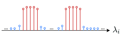
Figure 4: The spatial indices can be divided into two groups according to $\lambda_{i}$.

Algorithm 2 Obtaining the non-zero supporting vector from $\boldsymbol{\lambda}$ through k-Means algorithm

0:  : $\boldsymbol{\lambda}$.

0:  : $\mathcal{O}$

1:  $\lambda_{c1}=\max(\boldsymbol{\lambda})$, $\lambda_{c2}=\min(\boldsymbol{\lambda}_{k})$,

2:  repeat

3:     $i=1$ , $\mathcal{O}=\emptyset$ , $\mathcal{O}^{\prime}=\emptyset$

4:     repeat

5:        if $|\lambda_{i}-\lambda_{c1}|>|\lambda_{i}-\lambda_{c2}|$ then

6:           $\mathcal{O}=\mathcal{O}\cup\{i\}$

7:        else

8:           $\mathcal{O}^{\prime}=\mathcal{O}^{\prime}\cup\{i\}$

9:        end if

10:        $\lambda_{c1}=\frac{1}{|\mathcal{O}|}\sum_{j\in\mathcal{O}}\lambda_{j}$, $~{}\lambda_{c2}=\frac{1}{|\mathcal{O}|}\sum_{j\in\mathcal{O}^{\prime}}\lambda_{j}$

11:     until $i=N$

12:  until $\mathcal{O}$ does not change.

III-F Obtain the Non-zero Supporting Vector from $\boldsymbol{\lambda}_{k}$

As mentioned in the Section II, the virtual channel $\mathbf{h}_{m}$ is sparse. Let us use the set $\mathcal{O}$ to collect the indices of the non-zero elements of $\mathbf{h}_{m}$ and refer to it as non-zero supporting vector, which is vital for the virtual channel tracking. As shown in Figure 4, the spatial indices can be clearly classified into two groups according to the value of $\lambda_{i}$. The two groups correspond to indices of zero elements and the none-zero elements, respectively. Based on these observations, we resort to the k-Means algorithm to efficiently extract spatial signature from $\boldsymbol{\lambda}$. The detailed steps are shown in Algorithm 2.

IV Virtual Channel Tracking And Model Mismatch Detection

Algorithm 3 Channel tracking through GAMP

0:  : Learned parameters $\hat{\alpha}$, $\hat{\boldsymbol{\lambda}}$ and the Set $\mathcal{Q}$. Training matrix D, and observation vectors $\mathbf{y}_{1}^{t}$, $\mathbf{y}_{2}^{t}$, …. The scalar estimation functions $g_{s}$ and $g_{\tilde{h}}$,and damping constants $\theta_{s}$,$\theta_{w}\in(0,1]$.

1:  Initialization: $m=1$, $\boldsymbol{\mu}^{t}_{f_{1}^{B}\to w_{1}}=0$, $\boldsymbol{\nu}^{t}_{f_{1}^{B}\to w_{1}}=[\hat{\boldsymbol{\lambda}}]_{\mathcal{O}}$.

2:  repeat

3:     $k=1$

4:     repeat

5:        Implement the forward message passing into the $m$th time block, i=0.

6:        repeat

7:           $i=i+1$

8:           $\mu^{t}_{f_{m,i}^{B}\to w_{m,i}}=\hat{\alpha}\left(\frac{\bar{\mu}^{t}_{f_{m-1,:}^{A}\to w_{m-1,i}}}{\bar{\nu}^{t}_{f_{m-1,:}^{A}\to w_{m-1,i}}}+\frac{\mu^{t}_{f_{m-1,i}^{B}\to w_{m-1,i}}}{\nu^{t}_{f_{m-1,i}^{B}\to w_{m-1,i}}}\right)\frac{\bar{\nu}^{t}_{f_{m-1,:}^{A}\to w_{m-1,i}}\nu^{t}_{f_{m-1,i}^{B}\to w_{m-1,i}}}{\bar{\nu}^{t}_{f_{m-1,i}^{A}\to w_{m-1,i}}+\nu^{t}_{f_{m-1,i}^{B}\to w_{m-1,i}}}$.

9:           $\nu^{t}_{f_{m,i}^{B}\to w_{m,i}}=\left[\hat{\alpha}\right]^{2}\frac{\bar{\nu}^{t}_{f_{m-1,:}^{A}\to w_{m-1,i}}\nu^{t}_{f_{m-1,i}^{B}\to w_{m-1,i}}}{\bar{\nu}^{t}_{f_{m-1,:}^{A}\to w_{m-1,i}}+\nu^{t}_{f_{m-1,i}^{B}\to w_{m-1,i}}}+\left(1-\left[\hat{\alpha}\right]^{2}\right)\left[[\hat{\boldsymbol{\lambda}}]_{\mathcal{O}}\right]_{i}.$

10:        until $i=|\mathcal{O}|$

11:        Implement the message exchanging within the $m$th time block.

12:        GAMP:

13:        $\mathbf{A}=\mathbf{D}^{H}.\mathbf{D}^{H}$(component-wise magnitude squared)

14:        1./$\boldsymbol{\nu}_{p,m}^{t,(k)}=\mathbf{A}\boldsymbol{\nu}_{{w},m}^{t,(k)}$,$\mathbf{p}_{m}^{t,(k)}=\mathbf{s}_{m}^{t,(k-1)}+\boldsymbol{\nu}_{p,m}^{t,(k)}.\mathbf{D}^{H}\mathbf{w}_{m}^{t,(k)}$.

15:        $\boldsymbol{\nu}_{s,m}^{t,(k)}=\boldsymbol{\nu}_{p,m}^{t,(k)}.g_{s}^{\prime}\left(\mathbf{p}_{m}^{{t,(k)}},\boldsymbol{\nu}_{p,m}^{t,(k)}\right)$, $\mathbf{s}_{m}^{t,(k)}=(1-\theta_{s})\mathbf{s}_{m}^{t,(k-1)}+\theta_{s}g_{s}\left(\mathbf{p}_{m}^{t,(k)},\boldsymbol{\nu}_{p,m}^{t,(k)}\right)$.

16:        1./${\boldsymbol{\nu}}_{r,m}^{t,(k)}=\mathbf{A}^{T}\boldsymbol{\nu}_{s,m}^{t,(k)}$,$\mathbf{r}_{m}^{t,(k)}=\mathbf{w}_{m}^{t,(k)}-\boldsymbol{\nu}_{r,m}^{t,(k)}.\mathbf{D}\mathbf{s}_{m}^{t,(k)}$.

17:        $\boldsymbol{\tau}_{{w},m}^{t,(k+1)}=\boldsymbol{\nu}_{r,m}^{t,(k)}.g_{{w},m}^{\prime}(\mathbf{r}_{m}^{t,(k)},\boldsymbol{\nu}_{r,m}^{t,(k)})$,$\mathbf{w}_{m}^{t,(k+1)}=(1-\theta_{w})\mathbf{w}_{m}^{{t,(k)}}+\theta_{w}g_{{w},m}(\mathbf{r}_{m}^{t,(k)},\boldsymbol{\nu}_{r,m}^{t,(k)})$.

18:        GAMP END.

19:        for $i=1$ to $i=|\mathcal{O}|$, $\bar{\mu}^{t}_{f^{A}_{m,:}\to w_{m,i}}=[\mathbf{r}_{m}^{t,(k)}]_{i}$, $\bar{\nu}^{t}_{f^{A}_{m,:}\to w_{m,i}}=[\boldsymbol{\nu}_{r,m}^{t,(k)}]_{i}$.

20:        $k=k+1$

21:     until $k=K_{max}$

22:     $m=m+1$

23:  until The detection of the model mismatch.

24:  Output the tracking results of the $m$th block, i.e., $\hat{\textbf{w}}_{m}=\textbf{w}_{m}^{t,(K_{max}+1)},\boldsymbol{\Sigma}_{m}=\text{Diag}\left(\boldsymbol{\tau}_{w,m}^{t,(K_{max}+1)}\right)$.

After the channel parameter leaning, each user can obtain the information about $\boldsymbol{\Xi}=\{\alpha,\boldsymbol{\Lambda}\}$ and the corresponding supporting vector, denoted by $\mathcal{O}$. With the uplink feedback link, the BS can collect the channel characteristics for [35], BS implements the user grouping according to $\mathcal{O}$, and make sure that the supporting vectors for the users in the same group do not overlap. Thus, the users in the same group can reuse the same training sequence. In fact, after user grouping, for the user with $\mathcal{O}$, only $|\mathcal{O}|$ orthogonal training sequences are required. With respect to different users’ supporting index sets in one given group $\mathcal{G}_{g}$, let us assume the biggest cardinality among all the related sets as $P_{T}$. So, we can build a $P_{T}\times P_{T}$ matrix $\mathbf{T}_{g}$ with $\mathbf{T}_{g}\mathbf{T}_{g}^{H}=\frac{\sigma_{p}^{2}\mathbf{I}_{P_{T}}}{P_{T}}$ for this group, and select $|\mathcal{O}|$ rows of $\mathbf{T}_{g}$ to obtain $\mathbf{D}=[\mathbf{T}_{g}]_{1:|{{\mathcal{O}}}|,:}.$ Then, $\mathbf{D}$ is transmitted along the beam $[\mathbf{F}^{H}]_{:,\mathcal{O}}$, and the received signal at the user with $\mathcal{O}$ can be expressed as

$${\mathbf{y}}_{m}^{t}=\mathcal{Q}\{\mathbf{D}^{H}[\tilde{\mathbf{h}}_{m}^{t}]_{\mathcal{O}}+\mathbf{n}_{m}^{t}\},$$ (42)

where the superscript denotes that the related variable belongs to the tracking phase; $\mathbf{y}_{m}^{t}$, $\tilde{\mathbf{h}}_{m}^{t}$, and $\mathbf{n}_{m}^{t}$ separately have the same meaning with respect to $\mathbf{y}_{m}$, $\tilde{\mathbf{h}}_{m}$, and $\mathbf{n}_{m}$ in (20). Moreover, $\tilde{\mathbf{h}}_{m}$ and $\tilde{\mathbf{h}}_{m}^{t}$ (${\mathbf{n}}_{m}$ and ${\mathbf{n}}_{m}^{t}$) possess the same statistical characteristics. Then, we can obtain the following state-space model as

$$[\tilde{\mathbf{h}}_{m}^{t}]_{\mathcal{O}} =\hat{\alpha}[\tilde{\mathbf{h}}_{m}^{t}]_{\mathcal{O}}+\sqrt{1-\hat{\alpha}^{2}}\boldsymbol{\upsilon}_{m}^{t},$$ (43)

$${\mathbf{y}}_{m}^{t} =\mathcal{Q}\{\mathbf{D}^{H}[\tilde{\mathbf{h}}_{m}^{t}]_{\mathcal{O}}+\mathbf{n}_{m}^{t}\},.$$ (44)

where the statistical characteristics of $\boldsymbol{\upsilon}_{m}^{t}$ is the same with $\boldsymbol{\upsilon}_{m}$ in (19).

Obviously, we can resort to the proper nonlinear filtering, for example, the unscented Kalman filtering or the particle filtering, to track the virtual channel $\mathbf{w}_{m}=[\mathbf{\tilde{h}}_{m}^{t}]_{\mathcal{Q}}$. However, carefully analyzing the steps in Algorithm 1, we can find that the message scheduling process is similar to the operations in the Bayesian filtering and smoothing operations. Specially, the forward message passing is equivalent to the filtering, while the backward message passing is similar with the smoothing operation. Moreover, after parameter learning, the state-space model in (43) and (44) are low-dimensional without signal sparsity. Thus, with the above observations, we will construct one GAMP-based virtual channel tracking scheme in Algorithm 3. Notice that the notations $\mu^{t}_{f_{m,i}^{B}\to w_{m,i}}$, $\nu^{t}_{f_{m,i}^{B}\to w_{m,i}}$, ${\bar{\mu}}^{t}_{f_{m,i}^{A}\to w_{m,i}}$, ${\bar{\nu}}^{t}_{f_{m,i}^{A}\to w_{m,i}}$ in Algorithm 3 has the similar meaning to $\mu_{f_{m,i}^{B}\to{\tilde{h}}_{m,i}}$, $\nu_{f_{m,i}^{B}\to{\tilde{h}}_{m,i}}$, ${\bar{\mu}}_{f_{m,i}^{A}\to{\tilde{h}}_{m,i}}$, ${\bar{\nu}}_{f_{m,i}^{A}\to{\tilde{h}}_{m,i}}$ in Algorithm 1, respectively. Correspondingly, the explicit expressions for $g_{s}\left(\mathbf{p}^{t},\boldsymbol{\nu}_{\mathbf{p}}^{t}\right)$, $g_{w}(\mathbf{r}^{t},\boldsymbol{\nu}_{\mathbf{r}}^{t})$ can be inferred from $g_{s}\left(\mathbf{p},\boldsymbol{\nu}_{\mathbf{p}}\right)$, $g_{\tilde{h}}(\mathbf{r},\boldsymbol{\nu}_{\mathbf{r}})$ in Table. II through separately replacing ${\mu}_{f_{m,i}^{B}\to w_{m,i}}$, ${\nu}_{f_{m,i}^{B}\to w_{m,i}}$, ${\bar{\mu}}^{t}_{f_{m,i}^{A}\to w_{m,i}}$, ${\bar{\nu}}^{t}_{f_{m,i}^{A}\to w_{m,i}}$ by $\mu^{t}_{f_{m,i}^{B}\to w_{m,i}}$, $\nu^{t}_{f_{m,i}^{B}\to w_{m,i}}$, ${\bar{\mu}}^{t}_{f_{m,i}^{A}\to w_{m,i}}$, ${\bar{\nu}}^{t}_{f_{m,i}^{A}\to w_{m,i}}$.

Remark 1

Due to the mobility of the users and change of environment, the learned parameters will change in significant amounts. Thus, we have to start relearning process when the learned parameters mismatch with the real scenario. Here, we can resort to the Bayesian Cramér lower bound (BCRB) as the bench mark, which can be explained as follows. After achieving the channel model parameters, we can construct the tracking state space model as shown in (43) and (44), and derive the online BCRB. At every time block, we can get the virtual channel tracking MSE from the GAMP-based tracking scheme, which is denoted as $\boldsymbol{\Sigma}_{m}$ in Algorithm 3. When the tracking MSE is much higher than the corresponding BCRB, it is considered that the model parameters has changed and trigger the relearning process.

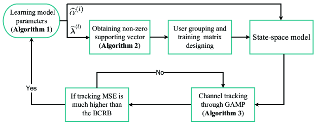
Figure 5: The overall block diagram of the proposed scheme.

In order to describe the relationship among different parts of the proposed scheme intuitively, the overall block diagram of the proposed scheme are illustrated in Figure 5.

V SIMULATION AND ANALYSIS

In this section, we evaluate the performance of our proposed scheme through numerical simulation. The number of antennas at the BS is $N=128$. The BS antenna spacing $d$ equals the half wavelength and the carrier frequency is 2GHz. The angular spread (AS) $\theta_{k}^{\text{max}}-\theta_{k}^{\text{min}}$ of the user is set as $4^{\circ}$ and the azimuth is randomly selected from $[-90^{\circ},90^{\circ}]$. We set the user’s velocity as 100 km/h. The signal-to-noise ratio (SNR) is defined as SNR$=\sigma_{p}^{2}/\sigma_{n}^{2}$. $M=32$ channel coherent blocks are used to learn the channel model parameters. The quantization step size is set according to [36]. Since the each of the users is independent during the down-link channel estimation, we only consider one user here.

The mean square error (MSE), which is formulated as follow, is taken as performance metrics.

$$\text{MSE}_{\mathbf{x}}= \frac{1}{M}\sum_{m=1}^{M}\frac{\|\hat{\mathbf{x}}_{m}-\mathbf{x}_{m}\|^{2}}{\|\mathbf{x}_{m}\|^{2}},{\mathbf{x}}=\alpha,\mathbf{\Lambda},{\tilde{\mathbf{h}}},{\mathbf{w}}.$$ (45)

V-A Model Parameters Learning

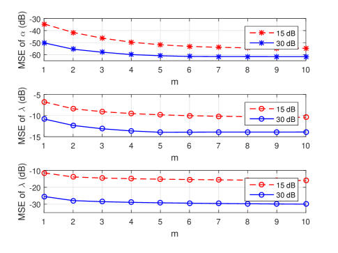
Figure 6: The convergence of the EM based model parameter learning algorithm (SNR=15dB and 30 dB).

We first investigate the convergence of the proposed GAMP-based model parameters learning scheme. The MSE curves versus the number of EM iteration is shown in Figure 6. The initial values are set as $\alpha_{k}=1$ and $\boldsymbol{\Lambda}_{k}=\mathbf{I}_{N}$ . It can be seen from Figure 6 that the EM algorithm takes 8 and 6 iterations to arrive at steady states for $\text{MSE}_{\alpha}$ and $\text{MSE}_{\boldsymbol{\Lambda}}$, respectively, under SNR = 15dB. When the SNR is 30dB, the convergence convergence speed is more faster. We can also see that the $\text{MSE}_{\alpha}$ of the first iteration can be as low as -50dB. This is not strange because $\alpha_{k}$ ranges from 1 to 0.9899 for a user with a velocity from $0$ km/h to $200$ km/h. Therefore, the initial value $\alpha_{k}=1$ is pretty close to its true value.

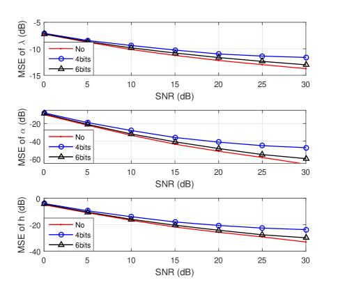
Figure 7: The MSE performance of the model parameters learning versus SNR.

Figure 7 presents the MSE of the model parameters learning as a function of the SNR. 10 iterations are used for the EM algorithm. 4-bit quantization, 6-bit quantization and no quantization cases are considered. We can see that even in the low SNR range, the MSEs of $\alpha_{k}$ are very low while that of $\boldsymbol{\Lambda}_{k}$ is higher but still acceptable. It is also shown in Figure 7 that the MSE of 6-bit quantization is very close to that of no quantization, especially when the SNR is low. Howerver, the MSE gap between the quantization and no quantization increase with SNR. The reason behind this is that quantization will introduce some equivalent noise. Therefore, the higher the SNR, the greater the effect of quantization.

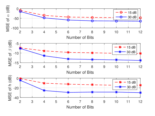
Figure 8: The MSE of the model parameters versus the number of quantization bits (SNR=15 and 30 dB).

To further reveal the quantization effects on the, we present the MSE performance of the model parametes learning versus the the number of quantization bits in Figure 8. When the number of quantization bits is small, the equivalent noise introduced by quantization is much higher than the noise. The MSE can be evidently reduced by increasing number of quantization bits . However, when the number of quantization bits is large, the equivalent noise introduced by quantization is much lower than the noise. The MSE is limited by the noise, especially when the SNR is low. Therefore, the MSE can not be deduced anymore by increasing number of quantization bits.

V-B Low-dimensional Virtual Channel Tracking

Under the framework of SBL, GAMP-based EM algorithm is used to learn the model parameters. After that, we will use the learned model parameters to achieve low-dimensional virtual channel tracking. Two examples of virtual channel tracking for no quantization and 6-bit quantization are presented in Figure 9 presents. It can be seen that the curves of the tracking result and true channel are closely entangled, which explicitly shown that the performance of proposed low-dimensional virtual channel tracking scheme is satisfactory.

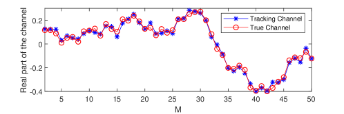
(a) No quantization.

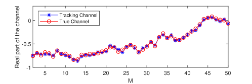
(b) 6-bits quantization.

Figure 9: Examples of channel tracking in the cases of non-quantization and 6-bits quantization.

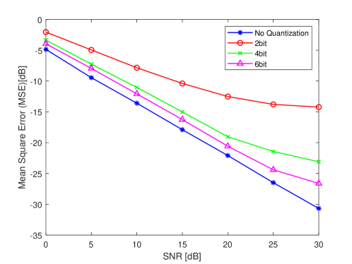
Figure 10: The performance of the virtual channel tracking versus SNR.

Then, we present the MSE of the proposed virtual channel tracking method as a function of SNR in Figure 10. The MSEs of 2-bit quantization, 4-bit quantization, 6-bit quantization and no quantization are compared. The performance trend over of virtual channel tracking likes that of model parameters learning. The MSEs of 6-bit quantization, 4-bit quantization and 2-bit quantization is close to that of no quantization when the SNR is low. Howerver, as the SNR increases, the MSE gaps between different quantization become more and more larger.

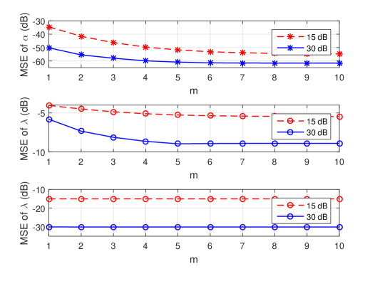
Figure 11: Comparison of the virtual channel tracking MSE and BCRB.

We display the virtual channel tracking MSE curves versus number of tracking time blocks in Figure 11. The online BCRB is also presented as the bench mark. It can be seen that both the BCRB and MSE initially decrease and eventually converge as the time block increases. This is because the time correlation of the channel is used, which can improve the tracking accuracy in the latter time block. It can be also seen that the curves in the case of SNR = 30db converge faster than in the case of SNR = 15dB. This is because the larger the SNR, the more gain of using time-correlation, so the earlier the convergence.

VI Conclusions

In this paper, we proposed a Bayesian downlink channel estimation algorithm for the time-varying massive MIMO networks. The effects of the quantization at the receiver are considered. Firstly, we developed an EM algorithm based SBL framework to learn the model parameters of the sparse virtual channel. Specifically, the factor graph and the GAMP algorithms were used to compute the desired posterior statistics in the E-step. Then, a reduced dimensional GAMP based scheme was proposed to track the virtual channel. From the simulation results, the proposed model parameters learning algorithm shows fast convergence speed. It takes 8 and 6 iterations to arrive at steady states for $\text{MSE}_{\alpha}$ and $\text{MSE}_{\boldsymbol{\Lambda}}$, respectively, under SNR = 15dB. When the SNR is higher, the convergence convergence speed is more faster. The proposed virtual channel tracking algorithm is able to make the full use of the channel temporal correlation and enhance the tracking accuracy.

Appenxdix A
Calculation of $p\Big{(}y_{m,p}|z_{m,p};\widehat{\boldsymbol{\Xi}}^{(l-1)}\Big{)}$ and $p\Big{(}\tilde{h}_{m,i}|\tilde{h}_{m-1,i};\widehat{\boldsymbol{\Xi}}^{(l-1)}\Big{)}$

Let us first consider the normal quantization in (7). From (20), it can be readily checked that $p\Big{(}q_{m,p}|z_{m,p};\widehat{\boldsymbol{\Xi}}^{(l-1)}\Big{)}=\mathcal{CN}\left(q_{m,p};{z_{m,p}},\sigma_{n}^{2}\right)$. Hence, it can be checked that

$$p\left(\Re\{q_{m,p}\}|\mathbf{\tilde{h}}_{m};\alpha\right)= \mathcal{N}\left(\Re\{q_{m,p}\};\Re\{z_{m,p}\},\frac{\sigma_{n}^{2}}{2}\right),$$ (46)

$$p\left(\Im\{q_{m,p}\}|\mathbf{\tilde{h}}_{m};\alpha\right)= \mathcal{N}\left(\Im\{q_{m,p}\};\Im\{z_{m,p}\},\frac{\sigma_{n}^{2}}{2}\right).$$ (47)

Before proceeding, let us define $\Phi(x)=\int^{x}_{-\infty}\frac{1}{\sqrt{2\pi}}e^{-\frac{u^{2}}{2}}du$. With the property of Gaussian distributions, the conditional PDF $p\Big{(}y_{m,p}|z_{m,p};\widehat{\boldsymbol{\Xi}}^{(l-1)}\Big{)}$ can be derived as

$$p\Big{(}y_{m,p}|z_{m,p};\widehat{\boldsymbol{\Xi}}^{(l-1)}\Big{)}= F\left(\Re\{y_{m,p}\}\right)F\left(\Im\{y_{m,p}\}\right)$$ (48)

where $F\left(\Re\{y_{m,p}\}\right)$ can be written as

$$F\left(\Re\{y_{m,p}\}\right)=\left\{\begin{aligned} &\Phi\left(\sqrt{2}\frac{(\Re\{y_{m,p}\}+\frac{1}{2})\triangle-\Re\{z_{m,p}\}}{\delta_{n}}\right)\ ,\ \Re\{y_{m,p}\}<-\frac{2^{\kappa}}{2}\\ &\Phi\left(\sqrt{2}\frac{(\Re\{y_{m,p}\}+\frac{1}{2})\triangle-\Re\{z_{m,p}\}}{\delta_{n}}\right)-\\ &\qquad\Phi\left(\sqrt{2}\frac{(\Re\{y_{m,p}\}-\frac{1}{2})\triangle-\Re\{z_{m,p}\}}{\delta_{n}}\right)\ ,\ -\frac{2^{\kappa}}{2}\leqslant\Re\{y_{m,p}\}\leqslant\frac{2^{\kappa}}{2}-1\\ &1-\Phi\left(\sqrt{2}\frac{(\Re\{y_{m,p}\}-\frac{1}{2})\triangle-\Re\{z_{m,p}\}}{\delta_{n}}\right)\ ,\ \Re\{y_{m,p}\}>\frac{2^{\kappa}}{2}-1\end{aligned}\right.,$$

and $F\left(\Im\{y_{m,p}\}\right)$ can be achieved through replacing $\Re\{y_{m,p}\}$ and $\Re\{z_{m,p}\}$ in (Appenxdix A Calculation of $p\Big{(}y_{m,p}|z_{m,p};\widehat{\boldsymbol{\Xi}}^{(l-1)}\Big{)}$ and $p\Big{(}\tilde{h}_{m,i}|\tilde{h}_{m-1,i};\widehat{\boldsymbol{\Xi}}^{(l-1)}\Big{)}$) with $\Im\{y_{m,p}\}$ and $\Im\{z_{m,p}\}$, respectively.

For the PDQ in (8), it can be derived that $y_{m,p}=(1-\rho)z_{m,p}+(1-\rho)n_{m,p}+n_{q,m,p}.$ Thus, $p\Big{(}y_{m,p}|z_{m,p};\widehat{\boldsymbol{\Xi}}^{(l-1)}\Big{)}$ can be denoted as

$$p\Big{(}y_{m,p}|z_{m,p};\widehat{\boldsymbol{\Xi}}^{(l-1)}\Big{)}=\mathcal{CN}(y_{m,p};(1-\rho)z_{m,p},(1-\rho)\sigma_{n}^{2}+\rho(1-\rho)).$$ (49)

From (19) it can be readily checked that

$$p\Big{(}\tilde{h}_{m,i}|\tilde{h}_{m-1,i};\widehat{\boldsymbol{\Xi}}^{(l-1)}\Big{)}\!=\!\left\{\begin{aligned} &\mathcal{CN}(\tilde{h}_{1,i};0,\lambda_{i}^{(l-1)}),&~{}m=1,\\ &\mathcal{CN}\left(\tilde{h}_{m,i};\hat{\alpha}^{(l-1)}\tilde{h}_{m-1,i},\Big{(}1-\Big{[}\hat{\alpha}^{(l-1)}\Big{]}^{2}\Big{)}\hat{\lambda}_{i}^{(l-1)}\right),&\text{otherwise}.\end{aligned}\right.$$ (50)

Appendix B
The derivation of $g_{s}\left(\mathbf{p},\boldsymbol{\nu}_{\mathbf{p}}\right)$ and $g_{\tilde{h}}(\mathbf{r},\boldsymbol{\nu}_{\mathbf{r}})$

In this appendix, we will derive the output scalar estimation function $g_{s}\left(\mathbf{p},\boldsymbol{\nu}_{\mathbf{p}}\right)$ and that for the input $g_{\tilde{h}}(\mathbf{r},\boldsymbol{\nu}_{\mathbf{r}})$, where the prior distribution ( 31) and the output function (30) will be utilized.

With respect to the input function $g_{\tilde{h}}(\mathbf{r},\boldsymbol{\nu}_{\mathbf{r}})$, it can be verified that it is not dependent on the quantization scenario. With (31) and (36) , it can be derived

$$\int{\tilde{h}}_{m,i}p({\tilde{h}}_{m,i})\mathcal{CN}({\tilde{h}}_{m,i};r_{i},\nu_{{r},i})d{\tilde{h}}_{m,i}$$

$$\!=\!\!\frac{\mu_{\{f^{B}_{m+1,i},f^{B}_{m,i}\}\to\tilde{h}_{m,i}}\nu_{{r},i}\!+\!r_{i}\nu_{\{f^{B}_{m+1,i},f^{B}_{m,i}\}\to\tilde{h}_{m,i}}}{\nu_{\{f^{B}_{m+1,i},f^{B}_{m,i}\}\to\tilde{h}_{m,i}}+\nu_{{r},i}}\mathcal{CN}\left(\mu_{\{f^{B}_{m+1,i},f^{B}_{m,i}\}\to\tilde{h}_{m,i}};r_{i},\nu_{\{f^{B}_{m+1,i},f^{B}_{m,i}\}\to\tilde{h}_{m,i}}+\nu_{{r},i}\right),$$ (51)

$$\int\!\!p({\tilde{h}}_{m,i})\mathcal{CN}({\tilde{h}}_{m,i};r_{i},\nu_{{r},i})d{\tilde{h}}_{m,i}=\mathcal{CN}\left(\mu_{\{f^{B}_{m+1,i},f^{B}_{m,i}\}\to\tilde{h}_{m,i}};r_{i},\nu_{\{f^{B}_{m+1,i},f^{B}_{m,i}\}\to\tilde{h}_{m,i}}+\nu_{{r},i}\right),\$$ (52)

where the property equation $\mathcal{CN}(x;\mu_{1},\nu_{1})\mathcal{CN}(x;\mu_{2},\nu_{2})=\mathcal{CN}(x;\frac{\mu_{1}/\nu_{1}+\mu_{2}/\nu_{2}}{1/\nu_{1}+1/\nu_{2}},\frac{1}{1/\nu_{1}+1/\nu_{2}})\mathcal{CN}(0;\mu_{1}-\mu_{2},\nu_{1}+\nu_{2})$ are utilized in the above derivations. Hence, the $i$th element of $g_{\tilde{h}}(\mathbf{r},\boldsymbol{\nu}_{\mathbf{r}})$ of $g_{\tilde{h}}^{\prime}(\mathbf{r},\boldsymbol{\nu}_{\mathbf{r}})$ can be separately written as

$$\left[g_{{\tilde{h}}}\left(\mathbf{r},\boldsymbol{\nu}_{\mathbf{r}}\right)\right]_{i}= \frac{\mu_{\{f^{B}_{m+1,i},f^{B}_{m,i}\}\to\tilde{h}_{m,i}}\nu_{{r},i}+r_{i}\nu_{\{f^{B}_{m+1,i},f^{B}_{m,i}\}\to\tilde{h}_{m,i}}}{\nu_{\{f^{B}_{m+1,i},f^{B}_{m,i}\}\to\tilde{h}_{m,i}}+\nu_{{r},i}},$$ (53)

$$\left[g_{{\tilde{h}}}^{\prime}\left(\mathbf{r},\boldsymbol{\nu}_{\mathbf{r}}\right)\right]_{i}= =\frac{\nu_{\{f^{B}_{m+1,i},f^{B}_{m,i}\}\to\tilde{h}_{m,i}}}{\nu_{\{f^{B}_{m+1,i},f^{B}_{m,i}\}\to\tilde{h}_{m,i}}+\nu_{{r},i}}.$$ (54)

The term $g_{s}\left(\mathbf{p},\boldsymbol{\nu}_{\mathbf{p}}\right)$ will be further examined. First, we will not consider the quantization effect, and can obtain $p(y_{m,p}|z_{m,p})=\mathcal{CN}(y_{m,p};z_{m,p},\sigma_{n}^{2})$. Then, from (35), we have

$$\int\!\!d{z}_{m,n}z_{m,n}p({y_{m,n}|z_{m,n}})\mathcal{CN}\left({z}_{m,n};\frac{p_{n}}{\nu_{p,n}},\frac{1}{\nu_{p,n}}\right)= \frac{\frac{y_{m,n}}{\sigma_{n}^{2}}+p_{n}}{\frac{1}{\sigma_{n}^{2}}+{\nu_{p,n}}}\mathcal{CN}\left(y_{m,n};\frac{p_{n}}{\nu_{p,n}},\sigma_{n}^{2}+\frac{1}{\nu_{p,n}}\right),$$ (55)

$$\int d{z}_{m,n}p({y_{m,n}|z_{m,n}})\mathcal{CN}\left({z}_{m,n};\frac{p_{n}}{\nu_{p,n}},\frac{1}{\nu_{p,n}}\right)= \mathcal{CN}\left(y_{m,n};\frac{p_{n}}{\nu_{p,n}},\sigma_{n}^{2}+\frac{1}{\nu_{p,n}}\right),$$ (56)

where the calculation techniques in (51) and ((52) ) are utilized in the above derivations. Then, the $n$th entry of $g_{s}\left(\mathbf{p},\boldsymbol{\nu}_{\mathbf{p}}\right)$ and $g_{s}^{\prime}\left(\mathbf{p},\boldsymbol{\nu}_{\mathbf{p}}\right)$ can be denoted as

$$\left[g_{\mathbf{s}}\left(\mathbf{p},\boldsymbol{\nu}_{\mathbf{p}}\right)\right]_{n}=\frac{p_{n}-\nu_{p,n}{y_{m,n}}}{1+\nu_{p,n}{\sigma_{n}^{2}}},\kern 20.0pt\left[g_{\mathbf{s}}^{\prime}\left(\mathbf{p},\boldsymbol{\nu}_{\mathbf{p}}\right)\right]_{n}=\frac{1}{1+\nu_{p,n}{\sigma_{n}^{2}}}.$$ (57)

Following the similar case, we can derive $g_{s}\left(\mathbf{p},\boldsymbol{\nu}_{\mathbf{p}}\right)$ and $g_{s}^{\prime}\left(\mathbf{p},\boldsymbol{\nu}_{\mathbf{p}}\right)$ under the PDQ scenario as

$$\left[g_{\mathbf{s}}\left(\mathbf{p},\boldsymbol{\nu}_{\mathbf{p}}\right)\right]_{n}= \frac{(1-\rho)p_{n}-\nu_{p,n}y_{m,n}}{(1-\rho)+\nu_{p,n}[(1-\rho)\sigma_{n}^{2}+\rho]},$$ (58)

$$\left[g_{\mathbf{s}}^{\prime}\left(\mathbf{p},\boldsymbol{\nu}_{\mathbf{p}}\right)\right]_{n}= \frac{1-\rho}{(1-\rho)+\nu_{p,n}[(1-\rho)\sigma_{n}^{2}+\rho]}.$$ (59)

With respect to the normal quantization case, we can obtain

$$\int p({y_{m,n}|z_{m,n}})\mathcal{CN}\left({z}_{m,n};\frac{p_{n}}{\nu_{p,n}},\frac{1}{\nu_{p,n}}\right)d{z}_{m,n}$$

$$=\int_{\epsilon_{\Re\{y_{m,n}\}}^{L}}^{\epsilon_{\Re\{y_{m,n}\}}^{U}}\int_{\epsilon_{\Im\{y_{m,n}\}}^{L}}^{\epsilon_{\Im\{y_{m,n}\}}^{U}}\mathcal{CN}\left({q}_{m,n};\frac{p_{n}}{\nu_{p,n}},\sigma_{n}^{2}+\frac{1}{\nu_{p,n}}\right)d{q}_{m,n}$$

$$=\left({\Phi(\zeta_{m,n})-\Phi(\eta_{m,n})}\right)\left({\Phi(\bar{\zeta}_{m,n})-\Phi(\bar{\eta}_{m,n})}\right),$$ (60)

where the terms $\zeta_{m,n}=\frac{\epsilon_{\Re\{y_{m,n}\}}^{U}-\frac{\Re\{p_{n}\}}{\nu_{p,n}}}{\sqrt{\frac{1}{2}\left(\sigma_{n}^{2}+\frac{1}{\nu_{p,n}}\right)}}$, $\eta_{m,n}=\frac{\epsilon_{\Re\{y_{m,n}\}}^{L}-\frac{\Re\{p_{n}\}}{\nu_{p,n}}}{\sqrt{\frac{1}{2}\left(\sigma_{n}^{2}+\frac{1}{\nu_{p,n}}\right)}}$, $\bar{\zeta}_{m,n}=\frac{\epsilon_{\Im\{y_{m,n}\}}^{U}-\frac{\Im\{p_{n}\}}{\nu_{p,n}}}{\sqrt{\frac{1}{2}\left(\sigma_{n}^{2}+\frac{1}{\nu_{p,n}}\right)}}$, $\bar{\eta}_{m,n}=\frac{\epsilon_{\Im\{y_{m,n}\}}^{L}-\frac{\Im\{p_{n}\}}{\nu_{p,n}}}{\sqrt{\frac{1}{2}\left(\sigma_{n}^{2}+\frac{1}{\nu_{p,n}}\right)}}$ are defined in the above equation.

Then, with respect to $\int z_{m,n}p({y_{m,n}|z_{m,n}})\mathcal{CN}\left({z}_{m,n};\frac{p_{n}}{\nu_{p,n}},\frac{1}{\nu_{p,n}}\right)d{z}_{m,n}$, we can obtain

$$\int z_{m,n}p({y_{m,n}|z_{m,n}})\mathcal{CN}\left({z}_{m,n};\frac{p_{n}}{\nu_{p,n}},\frac{1}{\nu_{p,n}}\right)d{z}_{m,n}$$

$$= \int_{\epsilon_{\Re\{y_{m,n}\}}^{L}}^{\epsilon_{\Re\{y_{m,n}\}}^{U}}\int_{\epsilon_{\Im\{y_{m,n}\}}^{L}}^{\epsilon_{\Im\{y_{m,n}\}}^{U}}\frac{{q}_{m,n}+\sigma_{n}^{2}p_{n}}{1+\sigma_{n}^{2}\nu_{p,n}}\mathcal{CN}\left({q}_{m,n};\frac{p_{n}}{\nu_{p,n}},\sigma_{n}^{2}+\frac{1}{\nu_{p,n}}\right)d{q}_{m,n}$$

$$= \frac{\left({\Phi(\zeta_{m,n})-\Phi(\eta_{m,n})}\right)\left({\Phi(\bar{\zeta}_{m,n})-\Phi(\bar{\eta}_{m,n})}\right)}{1+\sigma_{n}^{2}\nu_{p,n}}\left\{\left[\mathbb{E}_{\mathcal{TN}}\{\Re\{q_{m,n}\}\}+\jmath\mathbb{E}_{\mathcal{TN}}\{\Im\{q_{m,n}\}\}\right]+\sigma_{n}^{2}p_{n}\right\},$$ (61)

where both $\Re\{q_{m,n}\}$ and $\Im\{q_{m,n}\}$ are truncated normal distributed [37], and their PDFs are

$$p(\Re\{q_{m,n}\})= \mathcal{TN}\left(\Re\{q_{m,n}\};\frac{\Re\{p_{n}\}}{\nu_{p,n}},\frac{1}{2}\left(\sigma_{n}^{2}+\frac{1}{\nu_{p,n}}\right),\epsilon_{\Re\{y_{m,n}\}}^{L},\epsilon_{\Re\{y_{m,n}\}}^{U}\right),$$ (62)

$$p(\Im\{q_{m,n}\})= \mathcal{TN}\left(\Im\{q_{m,n}\};\frac{\Im\{p_{n}\}}{\nu_{p,n}},\frac{1}{2}\left(\sigma_{n}^{2}+\frac{1}{\nu_{p,n}}\right),\epsilon_{\Im\{y_{m,n}\}}^{L},\epsilon_{\Im\{y_{m,n}\}}^{U}\right).$$ (63)

Moreover, the notation $\mathcal{TN}(x;\mu,\nu^{2},a,b)$ denotes the real random variable $x$ is truncated normal distributed in the region $[a,b]$, where the non-truncated version of $x$ is normal distributed with mean $\mu$ and variance $\nu^{2}$. Plugging (60) and (61) into (35), we can obtain the $n$th element of $\left[g_{s}\left(\mathbf{p},\boldsymbol{\nu}_{p}\right)\right]_{n}$ under the normal quantization case as

$$\left[g_{s}\left(\mathbf{p},\boldsymbol{\nu}_{p}\right)\right]_{n}= p_{n}-\frac{\nu_{p,n}}{1+\sigma_{n}^{2}\nu_{p,n}}\left\{\left[\mathbb{E}_{\mathcal{TN}}\{\Re\{q_{m,n}\}\}+\jmath\mathbb{E}_{\mathcal{TN}}\{\Im\{q_{m,n}\}\}\right]+\sigma_{n}^{2}p_{n}\right\}.$$ (64)

With the theory of the truncated normal distribution, the following equation can be obtained

$$\int_{a}^{b}x\mathcal{TN}(x;\mu,\nu^{2},a,b)dx=\mu+\nu^{2}\frac{\mathcal{N}(a;\mu,\nu^{2})-\mathcal{N}(b;\mu,\nu^{2})}{\Phi\left(\frac{b-\mu}{\nu}\right)-\Phi\left(\frac{a-\mu}{\nu}\right)}.$$ (65)

With this property, we can rewrite (64) as

$$\left[\!g_{s}\!\left(\mathbf{p},\!\boldsymbol{\nu}_{p}\right)\!\right]_{n}\!\!= p_{n}\!\!-\!\!\frac{\nu_{p,n}}{1\!+\!\sigma_{n}^{2}\nu_{p,n}}\!\left\{\!\left[\mathbb{E}_{\mathcal{TN}}\{\Re\{q_{m,n}\}\}\!+\!\jmath\mathbb{E}_{\mathcal{TN}}\{\!\Im\{q_{m,n}\!\}\!\}\!\right]\!+\!\sigma_{n}^{2}p_{n}\right\}\!=\!\frac{1}{2}\!\frac{\Delta^{\Re}_{m,n}}{\nabla^{\Re}_{m,n}}\!\!+\!\!\frac{1}{2}\jmath\frac{\Delta^{\Im}_{m,n}}{\nabla^{\Im}_{m,n}},$$ (66)

where $\nabla^{\Re}_{m,n}={\Phi(\zeta_{m,n})-\Phi(\eta_{m,n})}$, $\nabla^{\Im}_{m,n}={\Phi(\bar{\zeta}_{m,n})-\Phi(\bar{\eta}_{m,n})}$, and $\Delta^{\Re}_{m,n}$, $\Delta^{\Im}_{m,n}$ can be separately written as

$$\Delta^{\Re}_{m,n}=\!\mathcal{N}\left(\epsilon_{\Re\{y_{m,n}\}}^{U};\frac{\Re\{p_{n}\}}{\nu_{p,n}},\frac{1}{2}\left(\sigma_{n}^{2}+\frac{1}{\nu_{p,n}}\right)\right)-\!\mathcal{N}\left(\epsilon_{\Re\{y_{m,n}\}}^{L};\frac{\Re\{p_{n}\}}{\nu_{p,n}},\frac{1}{2}\left(\sigma_{n}^{2}+\frac{1}{\nu_{p,n}}\right)\right),$$ (67)

$$\Delta^{\Im}_{m,n}=\!\mathcal{N}\left(\epsilon_{\Im\{y_{m,n}\}}^{U};\frac{\Im\{p_{n}\}}{\nu_{p,n}},\frac{1}{2}\left(\sigma_{n}^{2}+\frac{1}{\nu_{p,n}}\right)\right)-\!\mathcal{N}\left(\epsilon_{\Im\{y_{m,n}\}}^{L};\frac{\Im\{p_{n}\}}{\nu_{p,n}},\frac{1}{2}\left(\sigma_{n}^{2}+\frac{1}{\nu_{p,n}}\right)\right).$$ (68)

Thus, the $n$th element of $g_{s}^{\prime}\left(\mathbf{p},\boldsymbol{\nu}_{\mathbf{p}}\right)$ under the normal quantization case can be derived as

$$[g_{s}^{\prime}\left(\mathbf{p},\boldsymbol{\nu}_{\mathbf{p}}\right)]_{n}=\frac{1}{4}\Bigg{\{}\frac{\frac{\partial\Delta^{\Re}_{m,n}}{\partial\Re\{p_{n}\}}\nabla^{\Re}_{m,n}-\Delta^{\Re}_{m,n}\frac{\partial\nabla^{\Re}_{m,n}}{\partial\Re\{p_{n}\}}}{(\nabla^{\Re}_{m,n})^{2}}+\frac{\frac{\partial\Delta^{\Im}_{m,n}}{\partial\Im\{p_{n}\}}\nabla^{\Im}_{m,n}-\Delta^{\Im}_{m,n}\frac{\partial\nabla^{\Im}_{m,n}}{\partial\Im\{p_{n}\}}}{(\nabla^{\Im}_{m,n})^{2}}\Bigg{\}}.$$ (69)

After some calculations, we have

$$\frac{\partial\Delta^{\Re}_{m,n}}{\partial\Re\{p_{n}\}}\!=\!\!\frac{1}{\nu_{p,n}\sqrt{\!\!\frac{1}{2}\!\!\left(\!\!\sigma_{n}^{2}\!+\!\!\frac{1}{\nu_{p,n}}\!\!\right)}}\!\Big{(}\!\!\underbrace{\mathcal{N}\!\!\left(\!\epsilon_{\Re\{y_{m,n}\}}^{U};\!\frac{\Re\{p_{n}\}}{\nu_{p,\!n}},\!\frac{1}{2}\!\!\left(\!\sigma_{n}^{2}\!+\!\!\frac{1}{\nu_{p,n}}\!\!\right)\!\!\right)\zeta_{m,n}\!\!-\!\!\mathcal{N}\!\left(\!\epsilon_{\Re\{y_{m,n}\}}^{L};\frac{\Re\{\!p_{n}\}}{\nu_{p,n}},\frac{1}{2}\!\!\left(\!\sigma_{n}^{2}\!+\!\!\frac{1}{\nu_{p,n}}\!\!\right)\!\!\right)\eta_{m,n}}_{\Xi^{\Re}_{m,n}}\Big{)},$$

$$\frac{\partial\Delta^{\Im}_{m,n}}{\partial\Im\{p_{n}\}}\!=\!\!\frac{1}{\nu_{p,n}\sqrt{\frac{1}{2}\!\!\left(\!\sigma_{n}^{2}\!\!+\!\!\frac{1}{\nu_{p,\!n}}\!\!\right)}}\Big{(}\!\!\underbrace{\mathcal{N}\!\!\left(\!\!\epsilon_{\!\Im\{y_{m,n}\!\}}^{U};\!\!\frac{\Im\{p_{n}\}}{\nu_{p,n}},\frac{1}{2}\!\!\left(\!\!\sigma_{n}^{2}\!+\!\frac{1}{\nu_{p,n}}\!\!\right)\!\right)\bar{\zeta}_{m,n}\!-\!\mathcal{N}\!\!\left(\!\epsilon_{\Im\{y_{m,n}\}}^{L};\frac{\Im\{p_{n}\}}{\nu_{p,n}},\frac{1}{2}\!\!\left(\!\!\sigma_{n}^{2}\!\!+\!\!\frac{1}{\nu_{p,n}}\!\right)\!\right)\bar{\eta}_{m,n}}_{\Xi^{\Im}_{m,n}}\!\Big{)},$$

$$\frac{\partial\nabla^{\Re}_{m,n}}{\partial\Re\{p_{n}\}}=-\frac{1}{\nu_{p,n}}\underbrace{\left(\mathcal{N}\left(\epsilon_{\Re\{y_{m,n}\}}^{U};\frac{\Re\{p_{n}\}}{\nu_{p,n}},\frac{1}{2}\left(\sigma_{n}^{2}+\frac{1}{\nu_{p,n}}\right)\right)-\mathcal{N}\left(\epsilon_{\Re\{y_{m,n}\}}^{L};\frac{\Re\{p_{n}\}}{\nu_{p,n}},\frac{1}{2}\left(\sigma_{n}^{2}+\frac{1}{\nu_{p,n}}\right)\right)\right)}_{\Delta^{\Im}_{m,n}},$$

$$\frac{\partial\nabla^{\Im}_{m,n}}{\partial\Im\{p_{n}\}}=-\frac{1}{\nu_{p,n}}\underbrace{\left(\mathcal{N}\left(\epsilon_{\Im\{y_{m,n}\}}^{U};\frac{\Im\{p_{n}\}}{\nu_{p,n}},\frac{1}{2}\left(\sigma_{n}^{2}+\frac{1}{\nu_{p,n}}\right)\right)-\mathcal{N}\left(\epsilon_{\Im\{y_{m,n}\}}^{L};\frac{\Im\{p_{n}\}}{\nu_{p,n}},\frac{1}{2}\left(\sigma_{n}^{2}+\frac{1}{\nu_{p,n}}\right)\right)\right)}_{\Delta^{\Im}_{m,n}},$$

where the terms $\boldsymbol{\Xi}^{\Re}_{m,n}$ and $\boldsymbol{\Xi}^{\Im}_{m,n}$ are defined in the above equations. Substituting the above partial derivatives into (69), we can achieve

$$[g_{s}^{\prime}\left(\mathbf{p},\boldsymbol{\nu}_{\mathbf{p}}\right)]_{n}=\frac{1}{4\nu_{p,n}\sqrt{\frac{1}{2}\left(\sigma_{n}^{2}+\frac{1}{\nu_{p,n}}\right)}}\left\{\frac{\Xi^{\Re}_{m,n}}{\nabla^{\Re}_{m,n}}+\frac{\Xi^{\Im}_{m,n}}{\nabla^{\Im}_{m,n}}\right\}+\frac{1}{\nu_{p,n}}|\left[g_{s}\left(\mathbf{p},\boldsymbol{\nu}_{p}\right)\right]_{n}|^{2}$$ (70)

References

[1]
F. Rusek, D. Persson, B. K. Lau, E. G. Larsson, T. L. Marzetta, O. Edfors, and
F. Tufvesson, “Scaling up MIMO: Opportunities and challenges with very
large arrays,” IEEE Signal Process. Mag., vol. 30, no. 1, pp.
40–60, Jan. 2013.
[2]
V. Jungnickel, K. Manolakis, W. Zirwas, B. Panzner, V. Braun, M. Lossow,
M. Sternad, R. Apelfrojd, and T. Svensson, “The role of small cells,
coordinated multipoint, and massive MIMO in 5G,” IEEE Commun.
Mag., vol. 52, no. 5, pp. 44–51, May 2014.
[3]
F. Boccardi, R. W. Heath, A. Lozano, T. L. Marzetta, and P. Popovski, “Five
disruptive technology directions for 5G,” IEEE Commun. Mag.,
vol. 52, no. 2, pp. 74–80, Feb. 2014.
[4]
J. Hoydis, S. Ten Brink, and M. Debbah, “Massive MIMO in the UL/DL of
cellular networks: How many antennas do we need?” IEEE J. Sel. Areas
Commun., vol. 31, no. 2, pp. 160–171, Feb. 2013.
[5]
N. Jindal, “MIMO broadcast channels with finite-rate feedback,”
IEEE Trans. Inf. Theory, vol. 52, no. 11, pp. 5045–5060, Nov. 2006.
[6]
J. Choi, D. J. Love, and P. Bidigare, “Downlink training techniques for FDD
massive MIMO systems: Open-loop and closed-loop training with memory,”
IEEE J. Sel. Topics Signal Process., vol. 8, no. 5, pp. 802–814,
Oct. 2014.
[7]
S. Noh, M. D. Zoltowski, and D. J. Love, “Training sequence design for
feedback assisted hybrid beamforming in massive MIMO systems,”
IEEE Trans. Commun., vol. 64, no. 1, pp. 187–200, Jan. 2016.
[8]
Q. Zhang, S. Jin, K. K. Wong, H. Zhu, and M. Matthaiou, “Power scaling of
uplink massive MIMO systems with arbitrary-rank channel means,”
IEEE J. Sel. Topics Signal Process, vol. 8, no. 5, pp. 966–981,
Jan. 2014.
[9]
A. Adhikary, J. Nam, J.-Y. Ahn, and G. Caire, “Joint spatial division and
multiplexing the large-scale array regime,” IEEE Trans. Inf.
Theory, vol. 59, no. 10, pp. 6441–6463, Oct. 2013.
[10]
J. Nam, A. Adhikary, J. Y. Ahn, and G. Caire, “Joint spatial division and
multiplexing: Opportunistic beamforming, user grouping and simplified
downlink scheduling,” IEEE J. Sel. Topics Signal Process., vol. 8,
no. 5, pp. 876–890, Oct. 2014.
[11]
A. Adhikary, E. A. Safadi, M. K. Samimi, R. Wang, G. Caire, T. S. Rappaport,
and A. F. Molisch, “Joint spatial division and multiplexing for mm-Wave
channels,” IEEE J. Sel. Areas Commun., vol. 32, no. 6, pp.
1239–1255, Jun. 2014.
[12]
C. Sun, X. Gao, S. Jin, M. Matthaiou, Z. Ding, and C. Xiao, “Beam division
multiple access transmission for massive MIMO communications,”
IEEE Trans. Commun., vol. 63, no. 6, pp. 2170–2184, Jun. 2015.
[13]
A. Liu and V. Lau, “Phase only RF precoding for massive MIMO systems with
limited RF chains,” IEEE Trans. Signal Process., vol. 62, no. 17,
pp. 4505–4515, Sep. 2014.
[14]
J. Ma, S. Zhang, H. Li, N. Zhao, and V. C. M. Leung, “Interference-alignment
and soft-space-reuse based cooperative transmission for multi-cell massive
mimo networks,” IEEE Trans. Wireless Commun., vol. 17, no. 3, pp.
1907–1922, Mar. 2018.
[15]
Z. Gao, L. Dai, W. Dai, and Z. Wang, “Block compressive channel
estimation and feedback for FDD massive MIMO,” in Proc. IEEE
Conference on Computer Communications Workshops (INFOCOM WKSHPS), Hong Kong,
China, April 2015.
[16]
Z. Gao, L. Dai, Z. Wang, and S. Chen, “Spatially common sparsity based
adaptive channel estimation and feedback for FDD massive MIMO,”
IEEE Trans. Signal Process., vol. 63, no. 23, pp. 6169–6183, Dec.
2015.
[17]
A. M. Sayeed, “Deconstructing multiantenna fading channels,” IEEE
Trans. Signal Process., vol. 50, no. 10, pp. 2563–2579, Oct. 2002.
[18]
D. Fan, F. Gao, G. Wang, Z. Zhong, and A. Nallanathan, “Angle domain signal
processing-aided channel estimation for indoor 60-GHz TDD/FDD massive
MIMO systems,” IEEE J. Sel. Areas Commun., vol. 35, no. 9, pp.
1948–1961, Sep. 2017.
[19]
J. Ma, S. Zhang, H. Li, F. Gao, and S. Jin, “Sparse bayesian
learning for the time-varying massive MIMO channels: Acquisition and
tracking,” IEEE Trans. Commun., vol. 67, no. 3, pp. 1925–1938,
Mar. 2019.
[20]
J. Zhao, F. Gao, W. Jia, J. Zhao, and W. Zhang, “Channel tracking for massive
MIMO systems with spatial-temporal basis expansion model,” in Proc.
IEEE International Conference on Communications (ICC), Paris, France, May
2017.
[21]
J. Chen and V. K. N. Lau, “Two-tier precoding for FDD multi-cell massive
MIMO time-varying interference networks,” IEEE J. Sel. Areas
Commun., vol. 32, no. 6, pp. 1230–1238, Jun. 2014.
[22]
G. M. Guvensen and E. Ayanoglu, “Beamspace aware adaptive channel estimation
for single-carrier time-varying massive MIMO channels,” in Proc.
IEEE International Conference on Communications (ICC), Paris, France, May
2017.
[23]
C. Wen, S. Jin, K. Wong, J. Chen, and P. Ting, “Channel estimation
for massive MIMO using gaussian-mixture bayesian learning,” IEEE
Trans. Wireless Commun., vol. 14, no. 3, pp. 1356–1368, Mar. 2015.
[24]
B. H. Fleury, “First- and second-order characterization of direction
dispersion and space selectivity in the radio channel,” IEEE Trans.
Inf. Theory, vol. 46, no. 6, pp. 2027–2044, Sep. 2000.
[25]
K. Liu, V. Raghavan, and A. M. Sayeed, “Capacity scaling and spectral
efficiency in wide-band correlated MIMO channels,” IEEE Trans.
Inf. Theory, vol. 49, no. 10, pp. 2504–2526, Oct. 2003.
[26]
J. Zhao, F. Gao, W. Jia, S. Zhang, S. Jin, and H. Lin, “Angle domain hybrid
precoding and channel tracking for millimeter wave massive MIMO systems,”
IEEE Trans. Wireless Commun., vol. 16, no. 10, pp. 6868–6880, Oct.
2017.
[27]
L. Fan, S. Jin, C. K. Wen, and H. Zhang, “Uplink achievable rate for massive
MIMO systems with low-resolution ADC,” IEEE Commun. Lett.,
vol. 19, no. 12, pp. 2186–2189, Mar. 2015.
[28]
F. Wang, J. Fang, H. Li, Z. Chen, and S. Li, “One-bit quantization
design and channel estimation for massive MIMO systems,” IEEE
Trans. Veh. Technol., vol. 67, no. 11, pp. 10 921–10 934, Nov. 2018.
[29]
H. Wang, C.-K. Wen, and S. Jin, “Bayesian optimal data detector for mmwave
ofdm system with low-resolution ADC,” IEEE J. Sel. Areas Commun.,
vol. 35, no. 9, pp. 1962–1979, Sep. 2017.
[30]
X. Yang and A. O. Fapojuwo, “Enhanced preamble detection for prach in LTE,”
in Proc. IEEE Wireless Communications and Networking Conference
(WCNC), Shanghai, China, April 2013.
[31]
E. G. Larsson and J. Li, “Preamble design for multiple-antenna OFDM-based
WLANs with null subcarriers,” IEEE Signal Process. Lett., vol. 8,
no. 11, pp. 285–288, Nov. 2001.
[32]
F. R. Kschischang, B. J. Frey, H.-A. Loeliger et al., “Factor graphs
and the sum-product algorithm,” IEEE Trans. Inf. Theory, vol. 47,
no. 2, pp. 498–519, Feb. 2001.
[33]
J. Ziniel, S. Rangan, and P. Schniter, “A generalized framework for learning
and recovery of structured sparse signals,” in Proc. IEEE Statistical
Signal Processing Workshop (SSP), Ann Arbor, MI, USA, Aug. 2012.
[34]
M. Al-Shoukairi, P. Schniter, and B. D. Rao, “A gamp-based low complexity
sparse bayesian learning algorithm,” IEEE Trans. Signal Process.,
vol. 66, no. 2, pp. 294–308, Jan. 2018.
[35]
H. Xie, F. Gao, S. Zhang, and S. Jin, “A unified transmission strategy for
TDD/FDD massive MIMO systems with spatial basis expansion model,”
IEEE Trans. Veh. Technol., vol. 66, no. 4, pp. 3170–3184, Apr.
2017.
[36]
T. Zhang, C. Wen, S. Jin, and T. Jiang, “Mixed-ADC massive MIMO
detectors: Performance analysis and design optimization,” IEEE
Trans. Wireless Commun., vol. 15, no. 11, pp. 7738–7752, Nov. 2016.
[37]
C. K. Williams and C. E. Rasmussen, Gaussian processes for machine
learning. MIT Press Cambridge, MA,
2006, vol. 2, no. 3.