Pin TQFT and Grassmann integral
Ryohei Kobayashi
| Institute for Solid State Physics, |
| University of Tokyo, Kashiwa, Chiba 277-8583, Japan |
We discuss a recipe to produce a lattice construction of fermionic phases of matter on unoriented manifolds. This is performed by extending the construction of spin TQFT via the Grassmann integral proposed by Gaiotto and Kapustin, to the unoriented pin± case. As an application, we construct gapped boundaries for time-reversal-invariant Gu-Wen fermionic SPT phases. In addition, we provide a lattice definition of (1+1)d pin- invertible theory whose partition function is the Arf-Brown-Kervaire invariant, which generates the classification of (1+1)d topological superconductors. We also compute the indicator formula of valued time-reversal anomaly for (2+1)d pin+ TQFT based on our construction.
1 Introduction and summary
The notion of fermionic topological phase of matter has attracted great interest, since fermionic systems admit novel phases that have no counterpart in bosonic systems [1, 2, 3, 4, 5, 6, 7, 8].
On orientable spacetime, fermionic topological phases are thought to be described at long distances by spin Topological Quantum Field Theory (spin TQFT). In [1], the authors provided a recipe to construct a state sum definition of spin TQFT, by formulating the spin theory called the Gu-Wen Grassmann integral on an oriented spin -manifold , equipped with a -form symmetry, whose partition function has the form
| (1.1) |
where is a background gauge field of the -form symmetry, and specifies a spin structure of , which is related to a 2-cocycle representing the second Stiefel-Whitney class as . is written in terms of a certain path integral of Grassmann variables defined by giving a triangulation of . (In the following, when there is no confusion, we simply write , , instead of , , etc.)
By studying the effect of re-triangulations and gauge transformations, this theory is shown to have an anomaly characterized by , where is the Steenrod square defined as . Then, one can construct a spin theory fully invariant under the change of triangulation and gauge transformations, by coupling the Grassmann integral with a non-spin theory called a “shadow theory” [9, 10], whose anomaly is again characterized by , and then gauging the -form symmetry,
| (1.2) |
In contrast, it is sometimes useful to consider a fermionic topological phase on an unoriented manifold [11, 12, 13, 14, 15], when the system has a symmetry that reverses the orientation of spacetime. In such a situation, the corresponding theory requires a pin structure, which encodes the orientation reversing symmetry. For instance, let us think of a (1+1)d topological superconductor in class BDI (characterized by time reversal symmetry with ), which follows a classification [16]. Cobordism theory [11, 17, 18] predicts that the classification is diagnosed by computing the partition function of the corresponding TQFT on an unoriented surface equipped with a pin- structure. As another example, the (3+1)d topological superconductor in class DIII (time reversal symmetry with ) is known to be classified by [5, 19, 20, 21]. The classification is detected by the partition function of the TQFT on , equipped with a pin+ structure. In this context, it is important to ask how to formulate the pin± TQFT on a manifold which is not necessarily oriented.
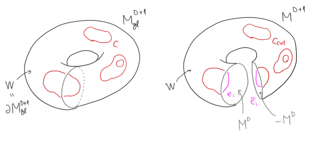
In this paper, we propose a strategy to produce a lattice definition of pin± TQFT in general dimensions, by extending the recipe in [1]. Concretely, we obtain the extended Grassmann integral on an unoriented -manifold . This is done by modifying the definition of the Grassmann integral properly, in the vicinity of the orientation reversing wall in , which flips the orientation as we go across the wall. We will show that the effect of re-triangulation and gauge transformation is expressed as
| (1.3) |
where is the same manifold with a different triangulation, is a cocycle such that in cohomology, and such that the two boundaries are given by and , and finally is extended to so that it restricts to and on the boundaries.
Then, we can define the pin- TQFT when admits a pin- structure, by coupling with a bosonic shadow theory which possesses an anomaly ,
| (1.4) |
where specifies a pin- structure that satisfies . We can also construct the pin+ TQFT when admits a pin+ structure, by coupling with a bosonic shadow theory with an anomaly ,
| (1.5) |
where specifies a pin+ structure that satisfies .
We have several applications of our construction of pin± TQFT based on the Grassmann integral. First, we construct the TQFT for a subclass of fermionic SPT phases known as pin± Gu-Wen -SPT phases [2, 1]. We further show that pin± Gu-Wen SPT phases always admit a gapped boundary, by explicitly constructing the Grassmann integral for the coupled bulk and boundary system on an unoriented manifold. In addition, we propose a lattice definition of 2d pin- TQFT whose partition function is the Arf-Brown-Kervaire (ABK) invariant [22, 23, 15], which generates the classification of (1+1)d topological superconductors. Finally, we discuss a way to compute the -valued (2+1)d pin+ anomaly from the data of (2+1)d anomalous theory. Such a formula for the anomaly (known as the indicator formula) has been conjectured in [24], and later proven in [21]. We compute the indicator formula when the anomalous theory is a pin+ TQFT whose shadow theory in the bulk is given by the (3+1)d Walker-Wang model [25]. Our indicator formula is expressed in terms of the data of the shadow TQFT.
This paper is organized as follows. In Sec. 2, we review the construction of the Grassmann integral for the oriented case, and describe the spin TQFT for the Gu-Wen SPT phase. In Sec. 3, we construct an extended Gu-Wen integral for unoriented manifolds, and describe the Gu-Wen -SPT phase based on the pin± structure. In Sec. 4, we propose a lattice construction of the ABK invariant based on the Grassmann integral. In Sec. 5, we construct gapped boundary theories for the Gu-Wen pin± -SPT phases. Finally, in Sec. 6, we compute the indicator formula for -valued anomaly of (2+1)d pin+ TQFT.
2 Review: Grassmann integral and Gu-Wen spin SPT phases
In this section, we first recall the construction of the Grassmann integral on an oriented spin -manifold formulated in [1]. Next, we describe the spin TQFT for fermionic Gu-Wen -SPT phases.
2.1 Review of the Gu-Wen Grassmann integral for spin case
We first endow with a triangulation. In addition, we take the barycentric subdivision for the triangulation of . Namely, each -simplex in the initial triangulation of is subdivided into simplices, whose vertices are barycenters of the subsets of vertices in the -simplex. We further assign a local ordering to vertices of the barycentric subdivision, such that a vertex on the barycenter of vertices is labeled as .
Each simplex can then be either a simplex or a simplex, depending on whether the ordering agrees with the orientation or not. We assign a pair of Grassmann variables on each -simplex of such that , we associate on one side of contained in one of -simplices neighboring (which will be specified later), on the other side. Then, is defined as
| (2.1) |
where denotes a -simplex, and is the product of Grassmann variables contained in . For instance, for , on is the product of . Here, denotes or depending on the choice of the assigning rule, which will be discussed later. The order of Grassmann variables in will also be defined shortly. We note that is ensured to be Grassmann-even when is closed.
Due to the fermionic sign of Grassmann variables, becomes a quadratic function, whose quadratic property depends on the order of Grassmann variables in . We will adopt the order used in Gaiotto-Kapustin [1], which is defined as follows.
-
•
For , we label a -simplex (i.e., a -simplex given by omitting a vertex ) simply as .
-
•
Then, the order of for -simplex is defined by first assigning even -simplices in ascending order, then odd simplices in ascending order again:
(2.2) -
•
For -simplices, the order is defined in opposite way:
(2.3)
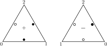
For example, for , when is a triangle, and for a triangle. Then, We choose the assignment of and on each such that, if is a (resp. ) simplex, includes when is labeled by an odd (resp. even) number, see Fig. 1.
Based on the above definition of , the quadratic property of is given by
| (2.4) |
for closed . To see this, we just have to bring the product of two Grassmann integrals
| (2.5) |
into the form of by permuting Grassmann variables, and count the net fermionic sign. First of all, each path integral measure on picks up a sign by permuting and . For integrands, on different -simplices commute with each other for closed , so nontrivial signs occur only by reordering to on a single -simplex. The sign on is explicitly written as
| (2.6) |
where the order is determined by . Hence, the net fermionic sign is given by
| (2.7) |
with
| (2.8) |
where if includes a variable. Then, the sign has a neat expression in terms of the higher cup product. For later convenience, we compute including the case that are not closed.
At a simplex, after some efforts we can rewrite as
| (2.9) |
The change of under the gauge transformation or under the change of the triangulation is controlled by the formula
| (2.11) |
where is the same manifold with a different triangulation, is a cocycle such that in cohomology, and such that the two boundaries are given by and , and finally is extended to so that it restricts to and on the boundaries. The derivation was given in [1].
We note that due to the Wu relation [26], we have
| (2.12) |
when is an oriented closed manifold and is a cocycle. This means that represents a trivial phase in dimensions, and therefore there should be a trivial boundary in dimensions. We can think of the Gu-Wen Grassmann integral as providing an explicit formula for such a trivial boundary.
2.2 Gu-Wen spin -SPT phase
The Gu-Wen spin invertible theories form a subgroup of and is specified by a pair satisfying , where . For a given where is a spin -manifold, the action of the invertible theory is given by [2, 1]111For a more mathematical treatment, see papers by Brumfiel and Morgan [27].
| (2.13) |
where is the Grassmann integral of Gu-Wen [2] as formulated by Gaiotto and Kapustin [1], and specifies the chosen spin structure.
3 Grassmann integral for pin case
Now let us construct the Grassmann integral on a -manifold which might be unoriented. We construct an unoriented manifold by picking locally oriented patches, and then gluing them along codimension one loci by transition functions. The locus where the transition functions are orientation reversing, constitutes a representative of the dual of first Stiefel-Whitney class . We will sometimes call the locus an orientation reversing wall. Again, we endow with a barycentric subdivision for the triangulation of . We then assign a local ordering to vertices of the barycentric subdivision, such that a vertex on the barycenter of vertices is labeled as .
For the oriented case, we have placed a pair of Grassmann variables on each -simplex , whose assignment is determined by the sign of -simplices () sharing . We remark that the assigning rule fails, when lies on the wall where we glue patches of by the orientation reversing map. In this case, we would have to assign Grassmann variables of the same color on both sides of (i.e., both are black () or white ()), since the two -simplices sharing have the identical sign when is on the orientation reversing wall, see Fig. 2 (a). Hence, we need to slightly modify the construction of the Grassmann integral on the orientation reversing wall. To do this, instead of specifying a canonical rule to assign Grassmann variables on the wall, we just place a pair , on the wall in an arbitrary fashion. Then, we define the Grassmann integral as
| (3.1) |
where the term assigns weight (resp. ) on each -simplex on the orientation reversing wall, when is shared with (resp. ) -simplices. There is no ambiguity in such definition, since both -simplices on the side of have the same sign. This factor makes the Grassmann integral a valued quadratic function. The quadratic property is expressed as
| (3.2) |
Basically, the quadratic property is derived in the similar fashion to the oriented spin case. In this case, the net sign consists of three parts;
-
•
the fermionic sign that occurs when reordering to on a single -simplex. The sign on is expressed as
(3.3) -
•
the fermionic sign by permuting the path integral measure, on each -simplex.
-
•
the sign that comes from factor on the wall, which is given by comparing with , with the sum of taken mod 2. This part counts on the orientation reversing wall.
Analogously to what we did to the second term in (2.8) for the oriented case, we try to re-distribute the fermionic sign from the measure to -simplices, by assigning to a simplex (resp. simplex) sharing , when is labeled by an odd (resp. even) number. However, such a distribution fails when is on the orientation reversing wall, due to the mismatch of the sign of two -simplices on the side of . Such a distribution counts no sign on the orientation reversing wall. But, this lack of the sign on the wall is complemented by the factor from the contribution of the term, making the re-distribution possible after all. Hence, we can express the net sign in exactly the same fashion as the oriented case (2.7), which proves (3.2).
3.1 Effect of re-triangulation
Next, we move on to discuss the effect of re-triangulation. Suppose we have two configurations of , orientation reversing walls and triangulations on and . Then, we will see that
| (3.4) |
where , and on , is extended to . To see this, we first observe the quadratic property of ,
| (3.5) |
Since (3.5) is satisfied for , we can express as up to linear term,
| (3.6) |
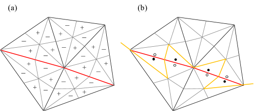
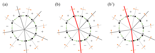
The linear term is fixed by computing in the simplest case; on , and on a single -simplex of , otherwise 0. Once we take a barycentric subdivision, when is nonzero away from the orientation reversing wall, one can see that , by imitating the logic of Sec. 4.1. of Gaiotto-Kapustin [1]. See also Fig. 3 (a). In the case that is nonzero on the orientation reversing wall, the value of depends on the way of assigning Grassmann variables to -simplices on the wall such that . For simplicity, we examine the case that is nonzero on two -simplices on the wall. (In general, there are even number of such -simplices. It is not hard to generalize for these situations.) Then, we have two Grassmann variables attached on each side of the orientation reversing wall. When the two Grassmann variables on one side of the wall share the same color (i.e., both are black () or white ()), we can show that (see Fig. 3 (b’)).
On the other hand, if the Grassmann variables on one side have different colors (i.e., one and one ), we have (see Fig. 3 (b)). (In these computations, the term spits no sign, .)
Now let us determine the linear term. First, let us recall that the set of all -simplices of the barycentric subdivision gives the representative of the dual of . Thus, we can express as
| (3.7) |
Here, if is nonzero away from the orientation reversing wall. When is nonzero on the wall, (resp. ) if the two Grassmann variables on one side of the wall have the same (resp. different) color. We can express such a linear term as . To see this, first we observe that the choice of the assignment of Grassmann variables on the wall corresponds to choosing the slight deformation of the wall, such that the deformation intersects transversally with the wall at -simplices. Concretely, we deform the wall on each -simplices of the wall to the side where (black dot) is contained, see Fig. 2 (b). Now we can see that when at the intersection of these two walls, otherwise 1. Here, both walls before and after deformation give a representative of the dual of , and thus the intersection of two walls gives a representative of the dual of . Hence, we have , proving (3.4).
3.2 Gu-Wen pin SPT phase
In this subsection, we discuss the fermionic SPT phases on an unoriented spacetime. To do this, let us begin with recalling the construction of bosonic SPT phases on unoriented manifolds, following [13]. Here, we limit ourselves to the case that the structure group is decomposed as . Then, the connection together with defines a connection of , , where is the subgroup of generated by the orientation reversing element. From now, we will simply write . We denote as a -action on , such that for , where when reverses the orientation, otherwise .
Then, a well-understood class of -dimensional bosonic SPT phases is classified by the -twisted cohomology group [28]. For a given , the action of the SPT phase on an unoriented -manifold is given by a certain product of weights on each -simplex of , which is constructed as follows.
First, let us consider the case that the -simplex is away from the orientation reversing wall. In this case, we simply define the weight as , where if is a simplex, and if is a simplex, which is identical to the definition of the oriented case. However, when the -simplex traverses the orientation reversing wall, the definition of the weight described above should be modified, since the choice of the sign has an ambiguity. To resolve such ambiguity, we first assign to every vertex of on one side of the wall, and assign on the other side. Then, we define as the sign given by comparing the ordering on and the orientation of on the side of vertices labeled by . Let us denote as the number assigned on the vertex of the smallest ordering in . Then, we define the weight on as .
We note that this definition is independent of the choice of assigning to one side of the wall, since flipping the sign of on vertices changes the sign of and simultaneously, which leaves invariant. Then, let us write the action as the product of weights for all -simplices in . We simply denote the action as . One can see that such defined action is invariant under re-triangulation [13]. If we take a general cochain which is not necessarily a cocycle, we can see that is no longer invariant under re-triangulation, whose variation is controlled by .
Now, we are ready to consider the fermionic case. The Gu-Wen SPT phase based on pin- structure is specified by a pair satisfying . For a given where is a pin- -manifold, the action of the invertible theory is given by
| (3.8) |
where specifies the chosen pin- structure.
On the other hand, the pin+ Gu-Wen SPT phase is given by such that . Here, we define such that , as a map that sends odd element of to 1, otherwise 0. Then, the action of the invertible theory is given in the form of (3.8), where specifies the chosen pin+ structure.
4 Arf-Brown-Kervaire invariant in (1+1)d
In this section, we construct the 2d pin- invertible TQFT [23] for the Arf-Brown-Kervaire (ABK) invariant via the Grassmann integral on lattice, whose state sum definition was initially given in [15]. In condensed matter literature, this invertible theory describes (1+1)d topological superconductors in class BDI [16]. Here, we construct the -valued ABK invariant by coupling the 2d state sum shadow TQFT with the Grassmann integral, which was performed for the -valued Arf invariant of the spin case in [1].
The weight for the state sum is assigned in the same manner as the case of the Arf invariant of the spin case [1], described as follows. For a given configuration , we assign weight to each 1-simplex , and also assign weight to each 2-simplex when at , otherwise 0. Let us denote the product of the whole weight as . Then, we can see that the partition function is given by the ABK invariant up to Euler term,
| (4.1) |
where , denotes the number of 2-simplices, 1-simplices in , respectively. denotes the Euler number of , and ABK is the ABK invariant,
| (4.2) |
Here, is a -valued quadratic function that satisfies
| (4.3) |
The ABK invariant determines the pin- bordism class of 2d manifolds , which is generated by [29]. To see this, let be a nontrivial 1-cocyle that generates . Then, using the quadratic property for in (4.3), one can see that takes value in , since and . corresponds to two possible choices of pin- structure on . Then, the ABK invariant is computed as an 8th root of unity,
| (4.4) |
5 Gapped boundary of Gu-Wen pin SPT phase
In this section, we demonstrate that Gu-Wen pin -SPT phases admit a gapped boundary, by writing down the explicit dimensional action on the boundary of dimensional Gu-Wen pin -SPT phase specified by the Gu-Wen data . To construct the gapped boundary, we prepare a symmetry extension by a (0-form) symmetry [30],
| (5.1) |
such that trivializes as an element of ; . When is finite, such an extension can be prepared by generalizing the argument of [31].
We now take such that . In pin- case, we see that is a (-twisted) cocycle, where . Therefore, the bulk Gu-Wen data pull back to . In pin+ case, we instead define the -twisted cocycle . Then, one can see that the Gu-Wen data pull back to .
Without loss of generality we can assume that for some , by a further extension of the symmetry
| (5.2) |
Again, such an extension for twisted cocycle can be prepared by generalizing the argument of [31]. We set . We now expect that the action on the boundary is given by the -gauge theory,
| (5.3) |
with . But to make sense of this expression we have to extend the definition of the Gu-Wen Grassmann integral to the case when is not necessarily closed. This generalization was performed for the spin case in [32]. By slightly generalizing the analysis in [32] to the pin case, we will see that the extended Gu-Wen integral nicely couples to the bulk in a gauge invariant fashion.
5.1 Bulk-boundary Gu-Wen Grassmann integral for the pin case
When we naively use the above definition (2.1) when is not closed: , the resulting expression is problematic since can become Grassmann-odd. Following [32], we avoid this conundrum by coupling with the Gu-Wen integral in dimensional bulk such that , making all components in the path integral Grassmann-even.
Now let us write down the boundary Gu-Wen integral coupled with bulk; we denote the entire integral by . We assign Grassmann variables on each -simplex of , and on each -simplex of . We define the Gu-Wen integral as
| (5.4) |
where we assume that the orientation reversing wall in intersects transversally at -simplices, which are regarded as making up the wall in . is a monomial of Grassmann variables defined on a -simplex of . is defined in the same fashion as in the case without boundary if is away from the boundary, but modified when shares a -simplex with the boundary. For simplicity, we assign an ordering on vertices of such , so that the -simplex shared with becomes ; the vertex is contained in . For instance, we can take a barycentric subdivision on , and assign to vertices associated with -simplices. We further define the sign of -simplices on , such that and have the same sign.
Then, neighboring with is defined by replacing the position of in with the boundary action on , . We then have: On a simplex,
| (5.5) |
On a simplex,
| (5.6) |
One can check that defined above becomes Grassmann-even. Then, using the exactly same logic as Sec. 4.3. of [32], one can obtain the quadratic property of as
| (5.7) |
5.2 Effect of re-triangulation
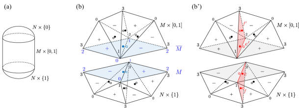
We can determine the effect of re-triangulation on from the quadratic property. To compare the value of the Gu-Wen integral on with different triangulations, we consider , with the Gu-Wen integral on , see Fig. 4 (a). Suppose we have two triangulations and configurations of we want to compare, on and , respectively. Roughly speaking, we will compute the effect of re-triangulations by showing that
| (5.8) |
and
| (5.9) |
To demonstrate these relations, we need to modify slightly the definition of and on the boundary . First, for -simplices in , we change the role of and in integrands, when is not contained in the orientation reversing wall. By this redefinition, the color of Grassmann variables away from the wall in match with that of , see Fig. 4 (b). Such a redefinition changes only by a linear and gauge invariant counterterm,
| (5.10) |
where denotes simplices on .
In addition, when is placed on the wall, we have to choose the assignment of Grassmann variables deliberately. Concretely, let be a simplex of on the side of . Then, we denote as a simplex of on the side of , which matches with by gluing and together. We also denote (resp. ) as a -simplex on the orientation reversing wall contained in (resp. ) respectively, which shares (resp. ). Then, we choose the assignment of , such that (see Fig. 4 (b’))
-
•
we place , on such that the color of the Grassmann variable on on one side of the orientation reversing wall coincides with that of .
-
•
we place on such that the color of the Grassmann variable on on one side of the orientation reversing wall differs from that of .
We emphasize that such redefinition or a specific choice of assignment does not affect the quadratic property (5.7). After these preparations, to see (5.8), we first observe the quadratic property of ,
| (5.11) |
which can be seen by applying quadratic property of (5.7) on , , . Note that (5.11) is satisfied for
| (5.12) |
where we set . Thus, we can express as up to linear term,
| (5.13) |
The linear term is fixed by computing explicitly in the simplest case; on , and on a single -simplex of , otherwise 0. If we take a barycentric subdivision on , we can see that when is nonzero on the dual of described in Sec. 3.1, at least if nonzero is away from the boundary of , , . When is nonzero on the boundary, we should be more careful. For instance, let be nonzero on . First, we discuss the case when is nonzero away from the orientation reversing wall of . Thanks to the above redefinition of , we can see that and have the opposite sign. Hence, we have . Next, let us examine the case when on the orientation reversing wall. Let , be two -simplices on the side of in the wall, which is contained in , , respectively. Then, one can see that , if the Grassmann variables on on one side of the wall have the same color, otherwise . Thus, now we can say that when is nonzero on the dual of of , even when lies in . Thus, we can fix the linear term as (5.8) up to linear and gauge invariant term.
Next, we demonstrate (5.9). Note that (5.7) is satisfied for
| (5.14) |
Thus, we can express as up to linear term,
| (5.15) |
Note that we are assuming that extends to . The linear term is again fixed by computing explicitly in the simplest case; on a single -simplex, otherwise 0. If we take a barycentric subdivision on , we can see that when is nonzero on the dual of described in Sec. 3.1, at least if is nonzero away from the boundary of . When is nonzero on the boundary, it requires more careful treatment. In this situation, by arranging the sign of chosen to be identical to , we can see that when is nonzero in away from the orientation reversing wall. Next, let us examine the case that is nonzero for contained in the orientation reversing wall. Let , be two -simplices on the side of in the wall, which is contained in , , respectively. Then, one can see that , if the Grassmann variables on on one side of the wall have the same color, otherwise , thanks to the choice of assignment of Grassmann variables in . Thus, now we can say that when is nonzero on the dual of of , even when lies in . Thus, we have the fixed the linear term as (5.9).
Combining (5.8) with (5.9), the variation of under re-triangulation and gauge transformation is given by
| (5.16) |
On the other hand, the variation of is given by
| (5.17) |
where specifies a pin- structure. Hence, the variation of the Grassmann integral becomes
| (5.18) |
In the pin+ case, the variation of is instead given by
| (5.19) |
5.3 Gapped boundary for the Gu-Wen pin phase
After all these preparations, it is a simple matter to show that the boundary gauge theory (5.3) correctly couples to the bulk Gu-Wen pin SPT phase. Indeed, the partition function of the coupled system has the action
| (5.20) |
for both pin- and pin+ case, where we take and . The first term in (5.20) has the variation (5.18) (resp. (5.19)) in pin- (resp. pin+) case, whereas the second term in (5.20) has the variation
| (5.21) |
These two variations cancel since we have (resp. ) and pulls back to (resp. ) in pin- (resp. pin+) case. This is what we wanted to achieve.
6 Time reversal anomaly of (2+1)d pin+ TQFT
In this final section, we apply our construction to the analysis of (2+1)d time reversal anomaly of class DIII, which is classified by [29].
In [19], the authors provided (presumably a bosonic shadow of) an anomalous theory based on the (3+1)d Walker-Wang model [25]. Their (3+1)d Walker-Wang model is constructed from a data of (2+1)d TQFT characterized by a premodular braided fusion category equipped with a transparent fermion, whose line operator generates a 1-form symmetry. By construction, the resulting (3+1)d Walker-Wang model admits a gapped boundary described by the given (2+1)d TQFT. Later, [24] conjectured the indicator formula that determines the -valued (2+1)d pin+ anomaly, from the data of (2+1)d TQFT realized on a boundary of the (3+1)d Walker-Wang model. The conjectured formula was demonstrated in [21], based on the argument that prepares the Hilbert space of pin+TQFT on a boundary of a non-orientable manifold.
The above background motivates us to revisit the indicator formula of the time-reversal anomaly in (2+1)d, by coupling the Walker-Wang model with the Grassmann integral we have constructed above. We aim to obtain the indicator formula for the anomaly, in terms of the data of the shadow TQFT. Suppose we have constructed the shadow of a (3+1)d pin+ SPT phase, described by a (3+1)d Walker-Wang model. Then, the Walker-Wang model is equipped with a line operator , which generates an anomalous 2-form symmetry characterized by
| (6.1) |
where is the background gauge field. Then, the invertible pin+ theory for an SPT phase is given by coupling with the Grassmann integral as
| (6.2) |
where denotes the partition function of the Walker-Wang model in the presence of the background 3-form gauge field. specifies a pin+ structure that satisfies . Since is generated by equipped with a pin+ structure, one should be able to construct the indicator formula by evaluating (6.2) for . In this case, we sum over , where a nontrivial element of corresponds to the insertion of a single line operator along a homotopically nontrivial line of . The Grassmann integral is again computed via the quadratic property (3.2),
| (6.3) |
When is a nontrivial element of , one can see that
| (6.4) |
Thus, we can show that mod 4, for a nontrivial . Such two choices of correspond to different choice of pin+ structure. Hence, the indicator formula has the form of
| (6.5) |
for nontrivial . Fortunately, the partition function of the Walker-Wang model on was explicitly computed in [33]. The result is expressed via the data of (2+1)d TQFT on boundary,
| (6.6) |
where is quantum dimension of , is total dimension characterized by , and is -valued topological spin of . denotes an orientation reserving symmetry, and is a quantity that characterizes the symmetry fractionalization of an anyon ; is defined as the eigenvalue of the symmetric state constructed on the Hilbert space on , where is implemented as the antipodal map of , and two anyons , are located on in an symmetric (i.e., antipodal) fashion. Namely, we have
| (6.7) |
In the first equation in (6.7), we note that permutes the position of two quasiparticles. The state exists only when fuse into vacuum; , otherwise becomes ill-defined. Accordingly, the summation runs over quasiparticles such that in (6.6).
By imitating the logic in [33], we can also compute for nontrivial background gauge field . In such a situation, the background field is realized as a single insertion of the transparent line operator , along a homotopically nontrivial loop in . As we examine in detail in Appendix A, the single insertion of an line amounts to evaluating the symmetry fractionalization on the Hilbert space on , in the presence of a single particle at the center of ; concretely, we prepare a symmetric state constructed on the Hilbert space on , where and lines fuse into an particle. The corresponding line ends at the center of . If we also denote the eigenvalue of such state as , the partition function in the presence of nontrivial background field is expressed as
| (6.8) |
where we sum over such that fuse into . After all, the indicator is expressed as
| (6.9) |
which reproduces the indicator formula proposed in [24], if we identify the above definition of as in [24]. 222Our definition of the total dimension is related to that of [24] by , since our total dimension counts the contribution of the transparent particle , while in [24] does not. The validity of such identification should be demonstrated for explicit lattice models, which is left for future work.
Acknowledgements
The author thanks Shinsei Ryu and Yuji Tachikawa for reading the draft of this paper and giving helpful suggestions and improvement. The author is grateful to Kantaro Ohmori, Shinsei Ryu, and Yuji Tachikawa for useful discussions. The author also acknowledges the hospitality of Kadanoff Center for Theoretical Physics. The author is supported by Advanced Leading Graduate Course for Photon Science (ALPS) of Japan Society for the Promotion of Science (JSPS).
Appendix A Partition function of the (3+1)d Walker-Wang model
In this appendix, following the logic of [33], we compute the partition function of the Walker-Wang model on , with or without background gauge field.
A.1 Gluing relation
We compute the partition function on a 4-manifold by decomposing the manifold into simpler manifolds for which partition functions are easier to evaluate and computing the partition function part by part. This procedure is performed via applying the gluing relation for the path integral. Here, let us review the application of the gluing relation to the Walker-Wang model, which is required for explicit computations, following Ref. [33, 34].
The data of (2+1)d TQFT (a braided fusion category ) defines a (3+1)d TQFT known as the Walker-Wang model. To consider the path integral of the Walker-Wang model on a 4d manifold , we first specify the configuration of fields on the boundary , where denotes a set of boundary conditions.
Here, the set of boundary conditions on a 3-manifold , , is defined as the set of all configurations of anyon diagrams on , based on the braided fusion category . If has boundary, we denote as the configuration space of anyon diagrams on , under the boundary condition on .
Then, the Hilbert space of the bulk-boundary coupled system is defined as the formal linear superposition of anyon diagrams , modded out by equivalence relations (e.g., fusions, and moves in ),
| (A.1) |
Then, the path integral is a map from to a number,
| (A.2) |
We will write the value as , for . The inner product in is defined via the bulk partition function as
| (A.3) |
where is a -manifold pinched at by the identification for and , so that . Furthermore, , specifies boundary conditions on , respectively, where denotes the field configuration on given by reversing the orientation of .
Now, let us describe the gluing relation. Let be a -manifold whose boundary is , and be a -manifold which is given by gluing the boundary of along and . Then, the partition function on with a boundary condition on is evaluated via the following gluing relation,
| (A.4) |
where is the boundary condition inherited from after the cut, and is the restriction of to . We denote an orthonormal basis of as . We illustrate the situation of the gluing relation in Fig. 5.
A.2 Handle decomposition of
Let us turn to the explicit computations of . We can compute the partition function on via gluing relations, by decomposing into simpler manifolds for which partition functions are easier to evaluate. To do this, we employ handle decomposition on , which takes apart into 4-balls.
For , a -handle in dimension is defined as a pair . is called an attaching region of the -handle. The 0-handle is defined as . We think of attaching a -handle to a -manifold with boundary, by an embedding of attaching region such that the image of is contained in . It is known that every compact -manifold without boundary allows a handle decomposition, i.e., is developed from a 0-handle by successively attaching to it handles of dimension .
We can see that is composed of single -handles for each by the following steps.
-
1.
To see this, it is convenient to think of as with its boundary identified by an antipodal map. First, we begin with locating a small 0-handle containing the center of .
-
2.
Next, we attach a 1-handle to the 0-handle. The attaching region of a 1-handle consists of two 3-balls, . We attach one of these s to the boundary of 0-handle, by identifying with a small in . Then, we radially extend a 1-handle from the attached , which tunnels through the antipodal map and returns to the 0-handle again. Eventually, we attach the other of the 1-handle to the 0-handle. We denote the composition of the handles in as . At this point, we have constructed .
-
3.
Then, we attach a 2-handle to . We note that , where is the action on defined as the composite of antipodal maps. The attaching region is embedded in , via embedding a small in .
-
4.
Likewise, we attach a 3-handle to by embedding the attaching region in , 333We note the abuse of notation; always denotes the composite of antipodal maps in this context. via embedding a small in .
-
5.
Finally, we complete with attaching a 4-handle to , by identifying the attaching region with .
A.3 Partition function on
Now we can compute by successively applying gluing relations in each process of the handle decomposition. In the presence of nontrivial background gauge field , amounts to inserting a single Wilson line of , along a loop in that intersects the crosscap of once. Here, we choose the configuration of , such that is contained in . runs in the direction of , living at the center of of . We denote the partition function on in the presence of such a line operator, simply as .
Then, the computation of proceeds as follows.
-
1.
First, we decompose into and a 4-handle, along the attaching region . Since there is no nontrivial anyon diagram on up to equivalence relations, only the empty diagram contributes to the boundary condition. Hence, the gluing relation becomes
(A.5) As shown in [33], we can see that and , where is the total dimension of anyons. Thus,
(A.6) - 2.
-
3.
Then, we decompose into and a 2-handle, along the attaching region . The boundary condition on the cut is labeled by the loop of anyon going around the . Gluing relation becomes
(A.10) Here, we have an line on going along , where denotes some point of . The notation means that the diagram has framing, as demonstrated in [33]. For , we have a bubble of loop on weighted by quantum dimension . Hence, . As shown in [33], we have , . Therefore,
(A.11) -
4.
Finally, we evaluate . is a twisted solid torus , where the twist is defined as an antipodal map of .
Let us recall the configuration of line operators for . First, we have an line on the boundary. The line on the boundary of looks like a worldline of a pair of anyon living in north and south pole of respectively, which is identified with each other at the twist. (Here, note that the antipodal map acts on anyon label as .)
Moreover, we have an line in the bulk living at the center of . To apply the gluing relation, we cut at a point of where we twist . On the cut section , we have a pair of anyons located in the antipodal fashion on the boundary, and also a single particle at the center of , see Fig. 6. We write the Hilbert space on the cut with such a configuration of anyons as . We note that such a state exist iff and fuse into . Then, the boundary condition on the section is a diagram which joins and together.
Now, recall that we have defined as the eigenvalue of the antipodal map on the state in . Since we operate the antipodal map when gluing the cut section , it picks up the eigenvalue by acting on the state of the section.
After all, when , the gluing relation becomes
(A.12) otherwise we have . Here, the framing contributes as topological spin of .
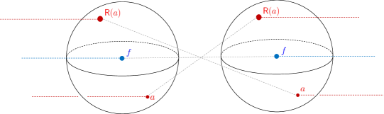
Figure 6: Configuration of anyons on the cut section . The antipodal map of acts on the state with particles .
References
- [1] D. Gaiotto and A. Kapustin, Spin TQFTs and Fermionic Phases of Matter, Int. J. Mod. Phys. A31 (2016) 1645044, arXiv:1505.05856 [cond-mat.str-el].
- [2] Z.-C. Gu and X.-G. Wen, Symmetry-protected topological orders for interacting fermions: Fermionic topological nonlinear models and a special group supercohomology theory, Phys. Rev. B90 (2014) 115141, arXiv:1201.2648 [cond-mat.str-el].
- [3] C. Wang, C. H. Lin, and Z. C. Gu, Interacting fermionic symmetry-protected topological phases in two dimensions, Physical Review B 95 (2017) 1–32, arXiv:1610.08478v1.
- [4] E. Witten, Fermion path integrals and topological phases, Reviews of Modern Physics 88 (2016) , arXiv:1508.04715v2.
- [5] M. A. Metlitski, L. Fidkowski, X. Chen, and A. Vishwanath, Interaction effects on 3D topological superconductors: surface topological order from vortex condensation, the 16 fold way and fermionic Kramers doublets, arXiv:1406.3032.
- [6] M. Cheng, Z. Bi, Y. Z. You, and Z. C. Gu, Classification of symmetry-protected phases for interacting fermions in two dimensions, Physical Review B 97 (2018) 1–11, arXiv:1501.01313v3.
- [7] Z. C. Gu, Z. Wang, and X. G. Wen, Lattice model for fermionic toric code, Physical Review B 90 (2014) 1–10, arXiv:1309.7032v3.
- [8] M. Guo, K. Ohmori, P. Putrov, Z. Wan, and J. Wang, Fermionic Finite-Group Gauge Theories and Interacting Symmetric/Crystalline Orders via Cobordisms, arXiv:1812.11959 [hep-th].
- [9] L. Bhardwaj, D. Gaiotto, and A. Kapustin, State sum constructions of spin-TFTs and string net constructions of fermionic phases of matter, Journal of High Energy Physics 2017 (2017) , arXiv:1605.01640v2.
- [10] T. D. Ellison and L. Fidkowski, Disentangling Interacting Symmetry-Protected Phases of Fermions in Two Dimensions, Physical Review X 9 (2019) 1–30, arXiv:1806.09623v3.
- [11] A. Kapustin, R. Thorngren, A. Turzillo, and Z. Wang, Fermionic Symmetry Protected Topological Phases and Cobordisms, JHEP 12 (2015) 052, arXiv:1406.7329 [cond-mat.str-el].
- [12] E. Witten, The "Parity" Anomaly on an Unorientable Manifold, Phys. Rev. B94 (2016) 195150, arXiv:1605.02391 [hep-th].
- [13] L. Bhardwaj, Unoriented 3d TFTs, Journal of High Energy Physics 2017 (2017) , arXiv:1611.02728v3.
- [14] H. Shapourian, K. Shiozaki, and S. Ryu, Many-Body Topological Invariants for Fermionic Symmetry-Protected Topological Phases, Physical Review Letters 118 (2017) 30–34, arXiv:1607.03896v3.
- [15] A. Turzillo, Diagrammatic State Sums for 2D Pin-Minus TQFTs, arXiv:1811.12654.
- [16] L. Fidkowski and A. Kitaev, Topological phases of fermions in one dimension, Physical Review B - Condensed Matter and Materials Physics 83 (2011) 1–14, arXiv:1008.4138v2.
- [17] D. S. Freed and M. J. Hopkins, Reflection Positivity and Invertible Topological Phases, arXiv:1604.06527 [hep-th].
- [18] K. Yonekura, On the Cobordism Classification of Symmetry Protected Topological Phases, arXiv:1803.10796 [hep-th].
- [19] L. Fidkowski, X. Chen, and A. Vishwanath, Non-Abelian topological order on the surface of a 3d topological superconductor from an exactly solved model, Physical Review X 3 (2014) , arXiv:1305.5851v4.
- [20] C. T. Hsieh, G. Y. Cho, and S. Ryu, Global anomalies on the surface of fermionic symmetry-protected topological phases in (3+1) dimensions, Physical Review B 93 (2016) 1–17, arXiv:1503.01411v4.
- [21] Y. Tachikawa and K. Yonekura, On time-reversal anomaly of 2+1d topological phases, Progress of Theoretical and Experimental Physics 2017 (2017) , arXiv:1611.01601v2.
- [22] E. H. Brown, Generalizations of the Kervaire invariant, Ann. Math. (1972) 368–383.
- [23] A. Debray and S. A. M. Gunningham, The Arf-Brown TQFT of pin- surfaces, arXiv:1803.11183v1.
- [24] C. Wang and M. Levin, Anomaly Indicators for Time-Reversal Symmetric Topological Orders, Physical Review Letters 119 (2017) 1–11, arXiv:1610.04624v1.
- [25] K. Walker and Z. Wang, (3+1)-TQFTs and topological insulators, arXiv:1104.2632v2.
- [26] Karlheinz Knapp, Wu class, http://www.map.mpim-bonn.mpg.de/Wu_class.
- [27] G. Brumfiel and J. Morgan, Quadratic Functions of Cocycles and Pin Structures, arXiv:1808.10484 [math.AT].
- [28] X. Chen, Z. C. Gu, Z. X. Liu, and X. G. Wen, Symmetry protected topological orders and the group cohomology of their symmetry group, Physical Review B 87 (2013) 1–55, arXiv:1106.4772v6.
- [29] R. Kirby and L. Taylor, Pin Structure on Low-dimensional Manifolds, Geometry of low-dimensional manifolds (1989) 177–242.
- [30] J. Wang, X.-G. Wen, and E. Witten, Symmetric Gapped Interfaces of SPT and SET States: Systematic Constructions, Phys. Rev. X8 (2018) 031048, arXiv:1705.06728 [cond-mat.str-el].
- [31] Y. Tachikawa, On Gauging Finite Subgroups, arXiv:1712.09542 [hep-th].
- [32] R. Kobayashi, K. Ohmori, and Y. Tachikawa, On gapped boundaries for SPT phases beyond group cohomology, arXiv:1905.05391.
- [33] M. Barkeshli, P. Bonderson, C.-M. Jian, M. Cheng, and K. Walker, Reflection and time reversal symmetry enriched topological phases of matter: path integrals, non-orientable manifolds, and anomalies, arXiv:1612.07792.
- [34] K. Walker, TQFTs [early incomplete draft] version 1h, http://canyon23.net/math/tc.pdf.