Convergence and Synchronization in Networks of Piecewise-Smooth Systems via Distributed Discontinuous Coupling

Abstract

Complex networks are a successful framework to describe collective behaviour in many applications, but a notable gap remains in the current literature, that of proving asymptotic convergence in networks of piecewise-smooth systems. Indeed, a wide variety of physical systems display discontinuous dynamics that change abruptly, including dry friction mechanical oscillators, electrical power converters, and biological neurons. In this paper, we study how to enforce global asymptotic state-synchronization in these networks. Specifically, we propose the addition of a distributed discontinuous coupling action to the commonly used diffusive coupling protocol. Moreover, we provide analytical estimates of the thresholds on the coupling gains required for convergence, and highlight the importance of a new connectivity measure, which we named minimum density. The theoretical results are illustrated by a set of representative examples.

, ,

1 Introduction

Complex networks have proven to be a powerful and effective paradigm to describe interaction and collective behaviour in networks of dynamical systems [1]. Yet, in the vast literature on synchronization of complex networks of the past 20 years, there is a notable gap: the case where the agents display discontinuous behaviour and therefore are modelled as piecewise-smooth (PWS) dynamical systems [16, 12, 28]. Importantly, differential equations with discontinuous right-hand sides appear in all applications featuring control systems with bang-bang, switched or hybrid controllers [37]. However, assessing whether coupling between agents will trigger synchronization in a network where the nodes are piecewise-smooth systems is still an open question. This is of crucial importance, for example, when the frequencies of multiple power generators must be synchronized in a smart grid with switching components [17, 36], or when ensuring convergence of the velocities of several interconnected mechanical components subject to dry friction [20, 27]. At the same time, spike synchronization in neurons has a crucial role in activities such as vision and motor coordination [18, 8, 7], while convergence of the motion of seismic faults leads the dreadful scenario of an earthquake [35, 5].

The reason why proving converge in a network of piecewise-smooth systems is a difficult task is twofold. Firstly, many common mathematical tools used when proving synchronization (e.g. Lyapunov approaches or the master stability function (MSF) technique [34]), in their standard form, require some degree of differentiability in the agents’ vector fields. Secondly, assumptions on the vector fields typically made for smooth systems, such as one-sided Lipschitz continuity and QUADness [15], cannot be exploited for PWS systems, but for a number of special cases. This fact also entails that, as discussed in [31], a linear diffusive coupling protocol (that is the most common communication protocol in complex networks) is not sufficient to guarantee convergence.

Numerous studies attempted to find alternative solutions to this problem. Early results on local synchronization between two coupled PWS systems were illustrated in [13], while the specific case of friction oscillators was discussed in [20]. More recently, an extension of the MSF technique to assess local stability of the synchronization manifold was presented in [8], even though, as explained in [26], such technique is only feasible for piecewise-smooth continuous [16] systems. Also, bounded synchronization between two coupled neural networks was investigated in [31], whereas more generic sufficient conditions for global bounded convergence to a synchronous solution were later given in [14]. Asymptotic synchronization was achieved via a leader-follower strategy in [40], where the authors exploited a control law injected at all the nodes to make the network track the state of a leader agent. However, this approach requires the presence of a single agent that can exert a centralised control action on all the systems (which is relatively costly and sometimes unfeasible) and the assumption that the trajectories of the open-loop network are bounded. So far, the only attempts at finding conditions to ensure global asymptotic convergence via a distributed coupling strategy (rather than a centralised controller) are illustrated in [29, 9]. In both papers strict assumptions (e.g. QUADness and semi-QUADness [29]) are made on the vector fields of the agents, excluding many PWS systems that do not satisfy them [14, 40, 30].

In this paper, we aim at finding sufficient conditions on the agent dynamics, the communication protocol and the structure of the interconnections in a network of piecewise-smooth systems so as to ensure global asymptotic convergence. We build on an intuition we presented in [9], where only a preliminary numerical investigation was carried out. Specifically, assuming the presence of a linear diffusive coupling protocol in the network, we propose a multiplex control approach [4], where communication among the nodes is extended via an additional discontinuous coupling layer, whose topology might differ from that of the diffusive one. Such an approach is corroborated by the evidence in the literature that some kind of discontinuous action is often required to enforce global convergence [31, 40]. In addition, discontinuous coupling protocols were already effectively used in different contexts. For example, they were exploited in [11, 24], to drive networks of integrators to consensus in finite time, and in [33, 38], using a hybrid system framework, to solve the problem of attitude synchronization among quaternions with smooth dynamics.

With the above multiplex distributed strategy, we advance the current state-of-the-art as follows.

1. We prove formally for the first time that asymptotic (rather than just bounded) synchronization in networks of piecewise-smooth systems is possible through the use of a distributed, multiplex coupling strategy;

2. We give analytical estimates of the critical values of both the coupling gains associated to the diffusive and the discontinuous layers, sufficient to guarantee global synchronization;

3. We show that the threshold value for the discontinuous coupling gain is dependent on a quantity we name minimum density of a graph, that acts as a connectivity measure, similarly to the well-known algebraic connectivity [21].

2 Notation and description of the problem

2.1 Notation

Given a vector $\bm{\xi}=[\xi_{1}\ \xi_{2}\ \cdots\ \xi_{n}]$, $\left\lvert\bm{\xi}\right\rvert=[\left\lvert\xi_{1}\right\rvert\ \left\lvert\xi_{2}\right\rvert\ \cdots\ \left\lvert\xi_{n}\right\rvert]$; $\mathrm{sign}(\bm{\xi})=[\mathrm{sign}(\xi_{1})\ \mathrm{sign}(\xi_{2})\ \cdots\ \mathrm{sign}(\xi_{n})]$; $\mathbf{i}_{i}\in\mathbb{R}^{n}$ is the column vector with $1$ in position $i$ and $0$ elsewhere; $\mathrm{diag}(\bm{\xi})$ is the diagonal matrix having the elements of vector $\bm{\xi}$ on its diagonal. $\left\lVert\cdot\right\rVert_{p}$ is the $p$-norm, and we recall that $\left\lVert\bm{\xi}\right\rVert_{1}\triangleq\sum_{i=1}^{n}\left\lvert\xi_{i}\right\rvert$.

Given a set $\mathcal{Q}$, if it is finite, we denote by $\left\lvert\mathcal{Q}\right\rvert$ its cardinality. For a set $\mathcal{Q}$ of scalars, the notation $\mathcal{Q}\leq 0$ means that $\forall\alpha\in\mathcal{Q}$, $\alpha\leq 0$ (analogously for $\geq$, $=$, etc.). $\mathcal{Q}\rightrightarrows\mathcal{R}$ denotes an application from $\mathcal{Q}$ to the set of all subsets of $\mathcal{R}$.

Given a matrix $\mathbf{A}$, we denote by $\lambda_{i}(\mathbf{A})$ its $i$-th eigenvalue, with eigenvalues being sorted in an increasing fashion if they are all real (so that $\lambda_{\mathrm{min}}(\mathbf{A})\triangleq\lambda_{1}(\mathbf{A})$). The notation $\mathbf{A}>0$ indicates that $\mathbf{A}$ is positive definite (analogously for semi- and negative definiteness); Finally, $\otimes$ is the Kronecker product. We recall that $\left\lVert\mathbf{A}\right\rVert_{\infty}\triangleq{\displaystyle\max_{i=1,\dots,n}}\left(\sum_{j=1}^{n}\left\lvert A_{ij}\right\rvert\right)$.

2.2 Problem description

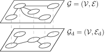
Figure 1: A multilayer network with $N=5$ and two coupling layers.

We consider the problem of finding conditions on the agent vector fields and an appropriate distributed control protocol $\mathbf{u}_{i}$ that can to make an ensemble of identical PWS systems of the form

$$\dot{\mathbf{x}}_{i}=\mathbf{f}(\mathbf{x}_{i};t)+\mathbf{u}_{i},\quad i=1,\dots,N$$ (1)

converge asymptotically towards a common evolution. Here $\mathbf{x}_{i}\in\mathbb{R}^{n}$, $t\in\mathbb{R}$ is time and $\mathbf{f}:\mathbb{R}^{n}\times\mathbb{R}\rightarrow\mathbb{R}^{n}$ is a generic piecewise-smooth vector field that might possibly exhibit sliding dynamics [16].

Definition 1 (Asymptotic synchronization).

Network (1) is asymptotically synchronized in $\Omega\subseteq\mathbb{R}^{nN}$ if, for all initial conditions in $\Omega$, $\lim_{t\rightarrow+\infty}\left\lVert\mathbf{x}_{i}(t)-\mathbf{x}_{j}(t)\right\rVert=0$, for all $i,j=1,\dots,N$. Moreover, network (1) is globally asymptotically synchronized if $\Omega=\mathbb{R}^{nN}$.

As shown in [14], a purely linear diffusive protocol does not suffice to achieve asymptotic convergence. Therefore, in this work we propose a multiplex control strategy [4] where an additional discontinuous coupling layer is added to a traditional linear diffusive one (see Figure 1). The two layers are associated to two undirected unweighted graphs: $\mathcal{G}=(\mathcal{V},\mathcal{E})$ associated to linear diffusive coupling, and $\mathcal{G}_{\mathrm{d}}=(\mathcal{V},\mathcal{E}_{\mathrm{d}})$ associated to discontinuous coupling; here, $\mathcal{V}$ is the set of vertices (or nodes) and $\mathcal{E},\mathcal{E}_{\mathrm{d}}$ are the set of edges (or links). Thus, our multilayer control action is given by

$$\mathbf{u}_{i}=-c\sum_{j=1}^{N}L_{ij}\bm{\Gamma}(\mathbf{x}_{j}-\mathbf{x}_{i})-c_{\mathrm{d}}\sum_{j=1}^{N}L_{ij}^{\mathrm{d}}\bm{\Gamma}_{\mathrm{d}}\mathrm{sign}(\mathbf{x}_{j}-\mathbf{x}_{i}),$$ (2)

for $i=1,\dots,N$, where $L_{ij}$ and $L_{ij}^{\mathrm{d}}$ are the $(i,j)$-th elements of the symmetric Laplacian matrices $\mathbf{L},\mathbf{L}_{\mathrm{d}}\in\mathbb{R}^{N\times N}$ associated to the graphs $\mathcal{G}$ and $\mathcal{G}_{\mathrm{d}}$, respectively; $\bm{\Gamma},\bm{\Gamma}_{\mathrm{d}}\in\mathbb{R}^{n\times n}$ are inner coupling matrices describing how the coupling actions affect the dynamics of the nodes.

3 Mathematical preliminaries

Let $\mathbf{A}\in\mathbb{R}^{n\times n}$ be a matrix and $\mu_{p}:\mathbb{R}^{n\times n}\rightarrow\mathbb{R}$ be the matrix measure (logarithimc norm) induced by the $p$-norm. We recall that $\mu_{2}(\mathbf{A})=\lambda_{\mathrm{max}}(\frac{\mathbf{A}+\mathbf{A}^{\mathsf{T}}}{2})$ and $\mu_{\infty}(\mathbf{A})=\max_{i}(A_{ii}+\sum_{j=1,j\neq i}^{n}\left\lvert A_{ij}\right\rvert).$ We denote $-\mu_{p}(-\mathbf{A})$ by $\mu_{p}^{-}(\mathbf{A})$, so that $\mu^{-}_{2}(\mathbf{A})=\lambda_{\mathrm{min}}(\frac{\mathbf{A}+\mathbf{A}^{\mathsf{T}}}{2}),$ and $\mu_{\infty}^{-}(\mathbf{A})=\min_{i}(A_{ii}-\sum_{j=1,j\neq i}^{n}\left\lvert A_{ij}\right\rvert).$ We also note that $\mu_{\infty}^{-}(\mathbf{I}_{m}\otimes\mathbf{A})=\mu_{\infty}^{-}(\mathbf{A})$, for any $m\in\mathbb{N}_{>0}$.

3.1 -QUAD property

We define next an extension to the well-known QUAD assumption, often used as a regularity condition on the internal agent dynamics in synchronization problems [15, 9].

Definition 2 (-QUAD).

A function $\mathbf{f}:\mathbb{R}^{n}\times\mathbb{R}\rightarrow\mathbb{R}^{n}$ is -QUAD($\mathbf{P}$, $\mathbf{Q}$, $\mathbf{M}$) if, $\forall\bm{\xi}_{1},\bm{\xi}_{2}\in\mathbb{R}^{n}$, $t\in\mathbb{R}$, $\exists\mathbf{P},\mathbf{Q},\mathbf{M}\in\mathbb{R}^{n\times n}$ such that

$$\left(\bm{\xi}_{1}-\bm{\xi}_{2}\right)^{\mathsf{T}}\mathbf{P}\left[\mathbf{f}(\bm{\xi}_{1};t)-\mathbf{f}(\bm{\xi}_{2};t)\right]\leq\left(\bm{\xi}_{1}-\bm{\xi}_{2}\right)^{\mathsf{T}}\mathbf{Q}\left(\bm{\xi}_{1}-\bm{\xi}_{2}\right)$$

$$+\left(\bm{\xi}_{1}-\bm{\xi}_{2}\right)^{\mathsf{T}}\mathbf{M}\ \mathrm{sign}\left(\bm{\xi}_{1}-\bm{\xi}_{2}\right).$$

Note that if $\mathbf{M}=\mathbf{0}_{n\times n}$, Definition 2 becomes equivalent to the classic QUAD condition. However, differently from the QUAD condition, the -QUAD property includes cases where $\mathbf{f}$ has any number of finite jumps discontinuities. Indeed, many real-world systems satisfy the -QUAD property (while failing to verify the QUAD assumption), featuring neuron models [8], gene regulatory networks [6], DC-DC converters, dry friction mechanical oscillators [20], and all QUAD systems controlled with bang-bang controllers [16]. As an illustrative example of what the -QUAD property implies, consider the functions $f_{1},f_{2}:\mathbb{R}\rightarrow\mathbb{R}$, given by $f_{1}(\xi)=\xi-\mathrm{sign}(\xi)$ and $f_{2}(\xi)=\xi+\mathrm{sign}(\xi)$, represented in Figure 2. $f_{1}$ is -QUAD with $\mathbf{P}=1$, $\mathbf{Q}=1$, $\mathbf{M}=0$, and thus is also QUAD; differently, $f_{2}$ is -QUAD with $\mathbf{P}=1$, $\mathbf{Q}=1$, $\mathbf{M}=2$, and can be proved not to be QUAD.

The following Lemma can be used to check for -QUADness. The proof immediately follows from the definitions of QUADness and -QUADness.

Lemma 3 (Evaluation of -QUADness).

Given a function $\mathbf{f}:\mathbb{R}^{n}\times\mathbb{R}\rightarrow\mathbb{R}^{n}$, if there exist $\mathbf{f}_{\mathrm{Q}}$ and $\mathbf{f}_{\mathrm{\sigma}}$ such that (i) $\mathbf{f}=\mathbf{f}_{\mathrm{Q}}+\mathbf{f}_{\mathrm{\sigma}}$, (ii) $\mathbf{f}_{\mathrm{Q}}$ is QUAD($\mathbf{P}$, $\mathbf{Q}$), and (iii) $\mathbf{f}_{\sigma}$ is bounded—i.e. $\exists\mathbf{m}\in\mathbb{R}^{n}:\left\lvert\mathbf{f}_{\sigma}(\bm{\xi}_{1})-\mathbf{f}_{\sigma}(\bm{\xi}_{2})\right\rvert\leq\mathbf{m}$, for all $\bm{\xi}_{1},\bm{\xi}_{2}\in\mathbb{R}^{n}$—then $\mathbf{f}$ is -QUAD($\mathbf{P}$, $\mathbf{Q}$, $\mathbf{M}$) with $\mathbf{M}=\mathrm{diag}(\left\lvert\mathbf{P}\right\rvert\mathbf{m})$.

Remark 4.

Lemma 3 allows to assess whether a PWS system with any number of finite jumps is -QUAD by only looking at its Jacobian, where it is defined. Indeed, if a vector field has a bounded Jacobian, then it also fulfils the QUAD assumption [10, Proposition 12].

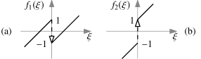
Figure 2: (a) $f_{1}$ is QUAD and -QUAD; (b) $f_{2}$ is not QUAD, but is -QUAD.

3.2 Network notation and definitions

With reference to network (1), (2), $\tilde{\mathbf{x}}\triangleq\sum_{i=1}^{N}\mathbf{x}_{i}/N\in\mathbb{R}^{n}$ is the average of the states of the nodes; $\mathbf{e}_{i}\triangleq\mathbf{x}_{i}-\tilde{\mathbf{x}}\in\mathbb{R}^{n}$, $i=1,\dots,N$ are the synchronization errors, and we denote the $h$-th element of $\mathbf{e}_{i}$ by $e_{i,h}$; $\bar{\mathbf{x}}\triangleq[\mathbf{x}_{1}^{\mathsf{T}}\ \cdots\ \mathbf{x}_{N}^{\mathsf{T}}]^{\mathsf{T}}\in\mathbb{R}^{nN}$ is the stack of the states of the nodes; $\bar{\mathbf{e}}\triangleq[\mathbf{e}_{1}^{\mathsf{T}}\ \cdots\ \mathbf{e}_{N}^{\mathsf{T}}]^{\mathsf{T}}\in\mathbb{R}^{nN}$ is the stack of the errors; $\mathbf{e}^{h}\triangleq[e_{1,h}\ \cdots\ e_{N,h}]^{\mathsf{T}}\in\mathbb{R}^{N}$ groups the $h$-th components of all the errors $\mathbf{e}_{i}$; $e_{\mathrm{tot}}\triangleq\frac{1}{N}\sum_{i=1}^{N}\left\lVert\mathbf{e}_{i}\right\rVert_{2}$ is the total synchronization error.

Given a graph $\mathcal{G}=\left\{\mathcal{V},\mathcal{E}\right\}$, we denote by $N$ the number of its vertices and by $N_{\mathcal{E}}$ be the number of its edges. A cut $\mathcal{C}$ is a partition of the set of vertices $\mathcal{V}$ in two subsets $\mathcal{V}_{1}$, $\mathcal{V}_{2}$; we name the sets of all possible cuts on $\mathcal{G}$ as $\hat{\mathcal{C}}_{\mathcal{G}}$, the number of edges that connect a vertex in $\mathcal{V}_{1}$ with one in $\mathcal{V}_{2}$ as $b$, and define the cardinalities $N_{1}=\left\lvert\mathcal{V}_{1}\right\rvert$, $N_{2}=\left\lvert\mathcal{V}_{2}\right\rvert$. In what follows, the ratio $b/N_{1}N_{2}$ represents the density of a cut $\mathcal{C}$.

Definition 5 (Minimum density).

The minimum density of a graph $\mathcal{G}$ is given by

$$\delta_{\mathcal{G}}\triangleq\frac{N}{2}\min_{\mathcal{C}\in\hat{\mathcal{C}}_{\mathcal{G}}}{\frac{b}{N_{1}N_{2}}}.$$ (3)

The optimal cut $\arg\min_{\mathcal{C}\in\hat{\mathcal{C}}_{\mathcal{G}}}\frac{b}{N_{1}N_{2}}$ associated to $\delta_{\mathcal{G}}$ is known as the sparsest cut [32], and is here denoted by $\mathcal{C}_{\text{sc}}$. The problem of finding such a cut is called the sparsest cut problem, which is a special kind of graph partitioning problem.

The sparsest cut problem is NP-hard and is normally solved algorithmically, as discussed below and in [2]. The minimum density of a graph can be computed using the free software METIS [25], which partitions the vertices into two subsets, minimising the number of edges between them, while keeping the sizes of the subsets to some fixed values. Specifically, we run METIS $\lfloor N/2\rfloor$ times, each time constraining $(N_{1},N_{2})$ to be $(1,N-1)$, then $(2,N-2)$ and so on until $(\lfloor N/2\rfloor,\lceil N/2\rceil)$. At each run, we compute $\frac{N}{2}\frac{b}{N_{1}N_{2}}$ and eventually choose the smallest value as the minimum density of the graph, according to Definition 5.

Note that the minimum density of some selected graph topologies can be computed analytically by relatively simple algebra. We report these findings in Table 1 (the proofs are omitted here for the sake of brevity).

Table 1: Values of the minimum density $\delta_{\mathcal{G}}$, the algebraic connectivity $\lambda_{2}(\mathbf{L})$ [19], and the number of edges $N_{\mathcal{E}}$ for selected topologies. “$l$-near.-n.” stands for “$l$-nearest-neighbours”; $\mathrm{c_{1}}\triangleq\cos{\left(\pi/N\right)}$, $\mathrm{c_{2}}\triangleq\cos{\left(2\pi/N\right)}$.

Topology	$\phantom{\begin{dcases}\end{dcases}}\delta_{\mathcal{G}}$	$\lambda_{2}(\mathbf{L})$	$N_{\mathcal{E}}$
Complete	$\phantom{\begin{dcases}\end{dcases}}N/2$	$N$	$\frac{N^{2}-N}{2}$
Star	$\phantom{\begin{dcases}\end{dcases}}N/(2(N-1))$	$1$	$N-1$
Path	$\begin{cases}2/N,&\text{$N$ even}\\ 2N/(N^{2}-1),&\text{$N$ odd}\end{cases}$	$2\left(1-\mathrm{c}_{1}\right)$	$N-1$
Ring	$\begin{cases}4/N,&\text{$N$ even}\\ 4N/(N^{2}-1),&\text{$N$ odd}\end{cases}$	$2\left(1-\mathrm{c}_{2}\right)$	$N$
$l$-near.-n.	$\begin{cases}\frac{4\sum_{k=0}^{l-1}(l-k)}{N},&\text{$N$ even}\\ \frac{4N\sum_{k=0}^{l-1}(l-k)}{N^{2}-1},&\text{$N$ odd}\end{cases}$	-	$Nl$

4 Convergence results

We expound next our main convergence results that allow to estimate the value of the critical coupling gains $c^{*}$ and $c_{\mathrm{d}}^{*}$ of the diffusive and discontinuous coupling layers, respectively, that guarantee global convergence of all agents towards a common synchronous evolution.

Theorem 6.

Network (1) controlled by the distributed multiplex control action (2) achieves global asymptotic synchronization if

1. there exist $\mathbf{P},\mathbf{Q},\mathbf{M}\in\mathbb{R}^{n\times n}$, with $\mathbf{P}>0$, such that (i) $\mathbf{f}$ is -QUAD($\mathbf{P}$, $\mathbf{Q}$, $\mathbf{M}$), (ii) $\mu_{2}^{-}(\mathbf{P}\bm{\Gamma})>0$, and $\mu_{\infty}^{-}(\mathbf{P}\bm{\Gamma}_{\mathrm{d}})>0$,

2. $\mathcal{G}$ and $\mathcal{G}_{\mathrm{d}}$ are connected graphs, and

3. $c>c^{*}$, $c_{\mathrm{d}}\geq c_{\mathrm{d}}^{*}$ with

   $$c^{*}\triangleq\frac{{\color[rgb]{0,0,0}\mu_{2}(\mathbf{Q})}}{\lambda_{2}(\mathbf{L})\ \ {\color[rgb]{0,0,0}\mu_{2}^{-}(\mathbf{P}\bm{\Gamma})}},\quad c^{*}_{\mathrm{d}}\triangleq\frac{{\color[rgb]{0,0,0}\mu_{\infty}(\mathbf{M})}}{\delta_{\mathcal{G}_{\mathrm{d}}}\ \ \mu_{\infty}^{-}(\mathbf{P}\bm{\Gamma}_{\mathrm{d}})}.$$ (4)

A proof of this theorem is given later in Section 6. Here, we wish to emphasise that the critical coupling gains $c^{*},c^{*}_{\mathrm{d}}$ depend on the internal node dynamics $\mathbf{f}$ through the matrices $\mathbf{Q}$, $\mathbf{P}$, $\mathbf{M}$, the inner coupling matrices $\bm{\Gamma}$, $\bm{\Gamma}_{\mathrm{d}}$, and the structure of the control layers $\mathbf{L}$, $\mathbf{L}_{\mathrm{d}}$ via the algebraic connectivity $\lambda_{2}(\mathbf{L})$ and the minimum density $\delta_{\mathcal{G}_{\mathrm{d}}}$. The multiplex nature of the strategy proposed here allows to pick the structure of each layer so as to fulfil a trade-off between the values of the required coupling gains and the number of edges in each layer (for some selected topologies, see Table 1).

Remark 7.

The results in Theorem 6 encompass the case of networks of smooth systems, whose global synchronization was characterised in [15]. As a matter of fact, in that case the systems would be -QUAD with $\mathbf{M}=\mathbf{0}$ (i.e. QUAD) and (4) would yield $c_{\mathrm{d}}^{*}=0$ and $c^{*}$ corresponding to [15, (H2)]. We also note that Theorem 6 accounts for the possible occurrence of sliding solutions, as explained in Section 6.4.2.

Concerning the evaluation of the conditions in Theorem 6, one possible way to assess -QUADness is through Lemma 3 and [10, Proposition 12]. Then, to estimate the algebraic connectivity $\lambda_{2}(\mathbf{L})$ it is possible to use methods such as that illustrated in [39]. As far as $\delta_{\mathcal{G}_{\mathrm{d}}}$ is concerned, to the best of our knowledge, no techniques to estimate it locally have been devised yet, which is reasonable though, since this is the first time this quantity is used in the context of network synchronization. Hence, until new estimation techniques are developed, it is advisable to compute $\delta_{\mathcal{G}_{\mathrm{d}}}$ through the algorithm or the formulae we provided in Section 3.2, and transmit this information to the nodes directly as a one-time operation. In addition, hypothesis (ii) holds if $\mathbf{P}\bm{\Gamma}>0$ and $\mathbf{P}\bm{\Gamma}_{\mathrm{d}}>0$, which in turn hold if $\bm{\Gamma}>0$, $\mathbf{P}\bm{\Gamma}=\bm{\Gamma}\mathbf{P}$, and $\bm{\Gamma}_{\mathrm{d}}>0$, $\mathbf{P}\bm{\Gamma}_{\mathrm{d}}=\bm{\Gamma}_{\mathrm{d}}\mathbf{P}$, which is as restrictive as other assumptions made in the literature on global synchronization (e.g. [40, 15, 29, 14]).

5 Examples

5.1 Achieving synchronization

We consider the problem of achieving global asymptotic synchronization in a network of $N=30$ piecewise-smooth relay systems with $\mathbf{f}(\mathbf{x}_{i})=\mathbf{A}\mathbf{x}_{i}-\mathbf{B}\mathrm{sign}(x_{i,1})$, where $\mathbf{A}=\left[\begin{smallmatrix}1.51&1&0\\ -99.922&0&1\\ -5&0&0\end{smallmatrix}\right]$ and $\mathbf{B}=[1\ -\!2\ 1]^{\mathsf{T}}$. Such systems naturally exhibit chaotic behaviour [16] and would not synchronize unless appropriately coupled. The internal dynamics $\mathbf{f}$ can be shown to be -QUAD according to Definition 2 through simple algebraic manipulations, with $\mathbf{P}=\mathbf{I}_{3}$, $\mathbf{Q}=\mathbf{A}$, and $\mathbf{M}=\left[\begin{smallmatrix}0&0&0\\ 4&0&0\\ 0&0&0\end{smallmatrix}\right]$; therefore ${\color[rgb]{0,0,0}\mu_{2}(\mathbf{Q})=50.312}$ and ${\color[rgb]{0,0,0}\mu_{\infty}(\mathbf{M})}=4$. We assume that the relays are coupled via two layers as in (2), with the structure of the diffusive layer, $\mathbf{L}$, corresponding to a ring graph, with $\lambda_{2}(\mathbf{L})=1$, while the structure of the discontinuous coupling layer, $\mathbf{L}_{\mathrm{d}}$, being chosen as the Erdős-Rényi-like graph shown in Figure 3a, with minimum density $\delta_{\mathcal{G}_{\mathrm{d}}}=1.290$. Figure 3b shows the sparsest cut of this latter graph, obtained numerically. We assume all states are available for coupling so that $\bm{\Gamma}=\bm{\Gamma}_{\mathrm{d}}=\mathbf{I}_{3}$; hence, ${\color[rgb]{0,0,0}\mu_{2}^{-}(\mathbf{P}\bm{\Gamma})}=\mu_{\infty}^{-}(\mathbf{P}\bm{\Gamma}_{\mathrm{d}})=1$. From Theorem 6, we can then compute the critical coupling gains that are sufficient for global convergence as ${\color[rgb]{0,0,0}c^{*}=50.312}$ and $c_{\mathrm{d}}^{*}=3.102$.

Figures 4a and 4b show the evolution of the total synchronization error $e_{\mathrm{tot}}$ (defined in Section 3) when the coupling gains are chosen below and above the critical threshold values. As expected from the theoretical results, when the gains are above the thresholds, the synchronization error converges asymptotically to zero. Note that the analytical estimates of the critical coupling gains are very conservative, as expected from a Lyapunov-based proof of convergence.

5.2 Assessing network resilence

Next, we show how the findings in Theorem 6 can be used to evaluate the resilience of the network with respect to structural changes in the communication layer. To this aim, consider the graph in Figure 3a having 82 edges and its sparsest cut in in Figure 3b. Assume that, due to some fault, 8 edges (roughly 10% of the total) are removed. We investigate two possible scenarios. In scenario A, 4 blue and 4 red intra-cluster edges are removed; the new graph in Figure 5a has minimum density $\delta_{\mathcal{G}_{\mathrm{A}}}=1.080$. In scenario B, 8 green inter-cluster edges are removed, with the new graph in Figure 5b having minimum density $\delta_{\mathcal{G}_{\mathrm{B}}}=0.747$. Consequently, from (4), the threshold value $c_{\mathrm{d}}^{*}$ associated to the latter graph will be larger (thus worse) than that associated to $\mathcal{G}_{\mathrm{A}}$. This suggests that the loss of resilience is greater when the inter-cluster edges (with respect to the sparsest cut of the original graph) are removed, although a detailed analysis of this effect is beyond the scope of this paper and will be the subject of future work.

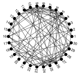
(a)

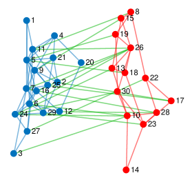
(b)

Figure 3: (a) Topology of the discontinuous coupling layer. The graph is an Erdős-Rényi-like one, with probability parameter $p=0.2$. (b) Sparsest cut of the topology in (a); $N_{1}=17$, $N_{2}=13$. $b=19$.

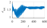
(a)

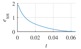
(b)

Figure 4: Error dynamics in a network of relay systems with (a) $c=0.1$, $c_{\mathrm{d}}=0.001$ and with (b) $c={\color[rgb]{0,0,0}51}$, $c_{\mathrm{d}}=3.200$.

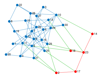
(a)

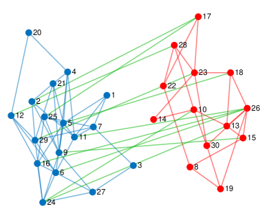
(b)

Figure 5: Graphs $\mathcal{G}_{\mathrm{A}}$ and $\mathcal{G}_{\mathrm{B}}$ obtained removing edges from the graph in Figure 3b. (a) 4 blue edges (2-9, 5-9, 6-11, 6-16) and 4 red edges (17-22, 18-26, 19-30, 23-28) from Figure 3b were removed; (b) 8 green edges (3-10, 5-19, 6-10, 7-26, 7-28, 8-11, 22-27, 24-30) from Figure 3b were removed.

6 Proofs

We give here the proofs of the convergence results presented in Section 4. We start by giving some lemmas and definitions in Section 6.1, we then introduce the concept of star functions in Section 6.2 and show how such functions can be associated to a given graph in Section 6.3. In particular, we show that semi-negativity of the star function for a given graph can be studied by assessing its value on the bipartitions of the graph. This allows to prove Theorem 6 in Section 4.

6.1 Preliminary lemmas and definitions

Definition 8 (Clusterization).

Given a vector $\bm{\xi}\in\mathbb{R}^{n}$, we define its clusterization, denoted by $\mathrm{clus}(\bm{\xi})$, as a partition of the set of indices $\mathcal{I}=\{1,\dots,n\}$, say $\{\mathcal{I}_{1},\dots,\mathcal{I}_{Q}\}$ with $1\leq Q\leq n$, such that, for all $i,j\in\mathcal{I}$, $\xi_{i}=\xi_{j}$ if and only if there exists $q\in(1,\dots,Q)$ such that $i,j\in\mathcal{I}_{q}$.

For example, according to this definition, the vector $\bm{\xi}=[1\ 1\ 6\ 2\ 2]^{\mathsf{T}}$ has a clusterization $\mathrm{clus}(\bm{\xi})=\{\mathcal{I}_{1},\mathcal{I}_{2},\mathcal{I}_{3}\}$ with $\mathcal{I}_{1}=\{1,2\},\mathcal{I}_{2}=\{3\},\mathcal{I}_{3}=\{4,5\}$. Clearly, the clusterization of a vector is unique up to a reordering of the clusters.

Lemma 9.

Given $\bm{\xi}\in\mathbb{R}^{n}$ and $\mathbf{A}\in\mathbb{R}^{n\times n}$, it holds that $\bm{\xi}^{\mathsf{T}}\mathbf{A}\mathrm{sign}(\bm{\xi})\leq{\color[rgb]{0,0,0}\mu_{\infty}(\mathbf{A})}\left\lVert\bm{\xi}\right\rVert_{1}$.

Defining $F\triangleq\bm{\xi}^{\mathsf{T}}\mathbf{A}\mathrm{sign}(\bm{\xi})$, we can write $F=\sum_{i=1}^{n}\left(A_{ii}\left\lvert\xi_{i}\right\rvert+\sum_{j=1,j\neq i}^{n}A_{ij}\xi_{i}\mathrm{sign}(\xi_{j})\right)$, then $F\leq\sum_{i=1}^{n}\left({\color[rgb]{0,0,0}A_{ii}}\left\lvert\xi_{i}\right\rvert+\sum_{j=1,j\neq i}^{n}\left\lvert A_{ij}\right\rvert\left\lvert\xi_{i}\right\rvert\right)$, and finally $F\leq\max_{i=1,\dots,n}\left({\color[rgb]{0,0,0}A_{ii}+\sum_{j=1,j\neq i}^{n}\left\lvert A_{ij}\right\rvert}\right)\sum_{i=1}^{n}\left\lvert\xi_{i}\right\rvert.$ ∎

Lemma 10.

Given $\bm{\xi}\in\mathbb{R}^{n}$ and $\mathbf{A}\in\mathbb{R}^{n\times n}$, it holds that $\bm{\xi}^{\mathsf{T}}\mathbf{A}\mathrm{sign}(\bm{\xi})\geq\mu_{\infty}^{-}(\mathbf{A})\left\lVert\bm{\xi}\right\rVert_{1}$, with $\mu_{\infty}^{-}$ given in Section 3.

Letting again $F\triangleq\bm{\xi}^{\mathsf{T}}\mathbf{A}\mathrm{sign}(\bm{\xi})$, we have $F\geq\sum_{i=1}^{n}\left(A_{ii}-\sum_{j=1,j\neq i}^{n}\left\lvert A_{ij}\right\rvert\right)\left\lvert\xi_{i}\right\rvert$, and $F\geq\min_{i=1,\dots,n}\left(A_{ii}-\sum_{j=1,j\neq i}^{n}\left\lvert A_{ij}\right\rvert\right)\sum_{i=1}^{n}\left\lvert\xi_{i}\right\rvert.$ ∎

Let $\mathbb{V}_{d}$ be a vector space in $\mathbb{R}^{d}$.

Definition 11 (Cones).

1. A set $\mathcal{K}\subseteq\mathbb{V}_{d}$ is a (convex) cone if, for any $\bm{\xi}_{1},\bm{\xi}_{2}\in\mathcal{K}$ and $\alpha_{1},\alpha_{2}\geq 0$, it holds that $\alpha_{1}\bm{\xi}_{1}+\alpha_{2}\bm{\xi}_{2}\in\mathcal{K}$.

2. A cone is finitely generated if it is the conical combination of a finite number of unit norm vectors, which we call generators of the cone.

3. A cone $\mathcal{K}$ is polyhedral if there exists a matrix $\mathbf{C}=[\mathbf{c}_{1}\ \mathbf{c}_{2}\ \cdots\ \mathbf{c}_{q}]\in\mathbb{R}^{d\times q}$ (with $q\geq d$ and $\mathbf{C}$ having rank $d$) such that $\mathbf{C}^{\mathsf{T}}\bm{\xi}\geq\mathbf{0}$, for all $\bm{\xi}\in\mathcal{K}$.

A finitely generated cone in $\mathbb{R}^{3}$ is illustrated in Figure 6a. Note that a convex cone contains its boundary.

Lemma 12 (Equivalence of cones [3]).

A polyhedral cone is a finitely generated cone having $p$ generators; the $i$-th generator $\hat{\bm{\xi}}_{i}$ is such that $\mathbf{c}_{j}^{\mathsf{T}}\hat{\bm{\xi}}_{i}=0$ for $n-1$ indices $j\neq i$. A finitely generated cone is also a polyhedral cone.

Definition 13 (Incidence matrix [21]).

The incidence matrix $\mathbf{B}\in\mathbb{Z}^{N\times N_{\mathcal{E}}}$ of a graph has columns $\mathbf{b}_{i}$, $i=1,\dots,N_{\mathcal{E}}$, where $\mathbf{b}_{i}$ is associated to edge $i$ connecting vertices $v_{j}$ and $v_{k}$, and has all its elements equal to zero, except for positions $j$ and $k$, where it has arbitrarily either $1$ and $-1$ or $-1$ and $1$.

Definition 14 (Bipartitions and tripartitions).

We term as bipartition (resp. tripartition) of a graph $\mathcal{G}$ the partition of the vertices set $\mathcal{V}$ in two (resp. three) subsets, also known as clusters, provided that at least two of the clusters are made of connected vertices.

We denote generic bipartitions by $\mathcal{B}=\{\mathcal{I}_{1},\mathcal{I}_{2}\}$ and tripartitions by $\mathcal{T}=\{\mathcal{I}_{1},\mathcal{I}_{2},\mathcal{I}_{3}\}$, where $\mathcal{I}_{i}$ is the set of indices of the vertices belonging to the $i$-th cluster. $\hat{\mathcal{B}}$ and $\hat{\mathcal{T}}$ denote the sets of all possible bipartitions and tripartitions, respectively. Finally, we define $\hat{\mathcal{P}}\triangleq\hat{\mathcal{B}}\cup\hat{\mathcal{T}}$ and a partition that is either a bipartition or a tripartition is denoted by $\mathcal{P}\in\hat{\mathcal{P}}$.

6.2 Star functions

Definition 15 (Star function).

A continuous piecewise-linear function $\phi:\mathbb{R}^{n}\rightarrow\mathbb{R}$ is a star function if (i) it is linear in a set of polyhedral convex cones $\mathcal{K}_{j}$, $j=1,\dots,J$, with $J\in\mathbb{N}_{>0}$, (ii) the cones can overlap only on their boundaries, and (iii) they are a cover for $\mathbb{R}^{n}$.

An example of the domain of a star function is illustrated in Figure 6b. We can now give the following Lemma, used to assess the semi-negativity of a star function.

(a)

(b)

Figure 6: (a) A finitely generated cone $\mathcal{K}_{j}$ in $\mathbb{R}^{3}$; $\hat{\bm{\xi}}_{1}$, $\hat{\bm{\xi}}_{2}$, and $\hat{\bm{\xi}}_{3}$ are the generators of the cone. (b) Example of the domain of a star function with 12 cones $\mathcal{K}_{j}$, $j=1,\dots,12$, in the case that $n=2$.

Lemma 16.

Given a star function $\phi:\mathbb{R}^{n}\rightarrow\mathbb{R}$, if $\phi(\bm{\xi})\leq 0$ on the generators of the cones $\mathcal{K}_{j}$, $j=1,\dots,J$ over which it is defined, then $\phi(\bm{\xi})\leq 0$ for all $\bm{\xi}\in\mathbb{R}^{n}$.

Without loss of generality, consider any cone $\mathcal{K}_{j}$ where $\phi$ is linear. Since, by definition $\mathcal{K}_{j}$ is a finitely generated cone, each of its points can be expressed as $\bm{\xi}=\alpha_{1}\hat{\bm{\xi}}_{1}+\alpha_{2}\hat{\bm{\xi}}_{2}+\ldots+\alpha_{p}\hat{\bm{\xi}}_{p},$ where $\hat{\bm{\xi}}_{1},\dots,\hat{\bm{\xi}}_{p}$ are the $p$ generators of $\mathcal{K}_{j}$, and $\alpha_{1},\dots,\alpha_{p}\geq 0$. Then, exploiting linearity of $\phi$, we have $\phi(\bm{\xi})=\alpha_{1}\phi(\hat{\bm{\xi}}_{1})+\alpha_{2}\phi(\hat{\bm{\xi}}_{2})+\ldots+\alpha_{n}\phi(\hat{\bm{\xi}}_{n})$, for all $\bm{\xi}\in\mathcal{K}_{j}$. Thus, since $\alpha_{1},\dots,\alpha_{p}\geq 0$, if $\phi$ is non-positive on all the generators $\hat{\bm{\xi}}_{i}$ of $\mathcal{K}_{j}$, then $\phi(\bm{\xi})\leq 0$ for all $\bm{\xi}\in\mathcal{K}_{j}$. The same is true for any other $\mathcal{K}_{j}$. ∎

6.3 Star function associated to a graph

Next we give a set of results concerning a specific type of star function that can be associated to a graph $\mathcal{G}$. We also show that the properties of this function can be interpreted in a graph-theoretical manner and derive some results that will be useful later in Section 6.4 to prove Theorem 6. We denote by $\mathcal{S}\subset\mathbb{R}^{N}$ the subspace $\mathcal{S}\triangleq\{\mathbf{e}\in\mathbb{R}^{N}\mid\sum_{i=1}^{N}e_{i}=0\}$. Then, we associate to a graph $\mathcal{G}$ the function $\phi_{\mathcal{G}}:\mathcal{S}\rightarrow\mathbb{R}$, given by

$$\phi_{\mathcal{G}}(\mathbf{e})=a_{1}\sum_{i=1}^{N}\left\lvert\mathbf{i}_{i}^{\mathsf{T}}\mathbf{e}\right\rvert-a_{2}\sum_{i=1}^{N_{\mathcal{E}}}\left\lvert\mathbf{b}_{i}^{\mathsf{T}}\mathbf{e}\right\rvert,$$ (5)

where $N$ and $N_{\mathcal{E}}$ are the numbers of vertices and edges in $\mathcal{G}$, respectively, $a_{1},a_{2}$ are positive scalars, $\mathbf{i}_{i}$ is the $i$-th vector of the canonical basis of $\mathbb{R}^{N}$, and $\mathbf{b}_{i}$ are the columns of the incidence matrix $\mathbf{B}$ of $\mathcal{G}$. It is not difficult to show that $\phi_{\mathcal{G}}$ is indeed a star function, although we omit these derivations for the sake of brevity. Each of its cones, say $\mathcal{K}_{j}$, is the locus where a vector constraint $\mathbf{C}_{j}^{\mathsf{T}}\mathbf{e}\geq\mathbf{0}$ holds, with

$$\mathbf{C}_{j}=\begin{bmatrix}\pm\mathbf{i}_{1}&\cdots&\pm\mathbf{i}_{N}&\pm\mathbf{b}_{1}&\cdots&\pm\mathbf{b}_{N_{\mathcal{E}}}\end{bmatrix},$$ (6)

and each cone $\mathcal{K}_{j}$ having a certain combination of plus and minus signs in place of the symbols $\pm$. We denote by $\hat{\mathcal{H}}\subset\mathcal{S}$ the set of all generators of $\phi_{\mathcal{G}}$.

Lemma 17.

Let $\mathcal{G}$ be a connected graph, $\phi_{\mathcal{G}}$ its associated star function defined as in (5), and $\hat{\mathbf{e}}\in\hat{\mathcal{H}}$ a generator of $\phi_{\mathcal{G}}$. The clusters $\mathcal{I}_{i}$ of indices in $\mathrm{clus}(\hat{\mathbf{e}})$ form either a bipartition or a tripartition of $\mathcal{G}$.

To prove the thesis, we need to show that (i) $\mathrm{clus}(\hat{\mathbf{e}})=\{\mathcal{I}_{1},\dots,\mathcal{I}_{Q}\}$ with $Q=2$ or $Q=3$; (ii) the partition of $\mathcal{G}$ contains at least two clusters of connected vertices.

(i)  From Lemma 12, it follows that any generator $\hat{\mathbf{e}}$ of $\phi_{\mathcal{G}}$ is a vector in $\mathcal{S}$ with unit norm such that $N-2$ independent constraints $\mathbf{c}_{i}^{\mathsf{T}}\hat{\mathbf{e}}=0$ hold. Recalling (6), we know that the vectors $\mathbf{c}_{i}$’s are picked from the set $\mathcal{C}_{\mathbf{i},\mathbf{b}}\triangleq\{\mathbf{i}_{1},\dots,\mathbf{i}_{N},\mathbf{b}_{1},\dots,\mathbf{b}_{N_{\mathcal{E}}}\}$. We term as $p$ the number of constraints of the form $\mathbf{i}_{i}^{\mathsf{T}}\hat{\mathbf{e}}=0$, so that those of the kind $\mathbf{b}_{i}^{\mathsf{T}}\hat{\mathbf{e}}=0$ are $N-2-p$, with $0\leq p\leq N-2$. According to the definition of $\mathbf{b}_{i}$, each of the constraints $\mathbf{b}_{i}^{\mathsf{T}}\hat{\mathbf{e}}=0$ implies that two components of $\hat{\mathbf{e}}$ are equal, i.e. that $\hat{e}_{j}=\hat{e}_{k}$, for some pair of indices $(j,k)$. Therefore, from the $N-2-p$ constraints of the form $\mathbf{b}_{i}^{\mathsf{T}}\hat{\mathbf{e}}=0$, we can conclude that $\mathrm{clus}(\mathbf{e})$ contains at most $N-(N-2-p)=p+2$ clusters. We need now to apply the remaining $p$ constraints of the form $\mathbf{i}_{i}^{\mathsf{T}}\hat{\mathbf{e}}=0$; we analyse separately the cases when $p=0$ or $p>0$.

• If $p=0$, there are no constraints like $\mathbf{i}_{i}^{\mathsf{T}}\hat{\mathbf{e}}=0$ to consider; thus, $\mathrm{clus}(\hat{\mathbf{e}})=\{\mathcal{I}_{1},\mathcal{I}_{2}\}$ with

  $$\begin{dcases}\hat{e}_{j}=\epsilon_{1},&j\in\mathcal{I}_{1},\\ \hat{e}_{j}=\epsilon_{2},&j\in\mathcal{I}_{2},\end{dcases}$$ (7)

  for some $\epsilon_{1},\epsilon_{2}\in\mathbb{R}$, with $\epsilon_{1},\epsilon_{2}\neq 0$ and $\epsilon_{1}\neq\epsilon_{2}$.

• If, on the other hand, $p>0$, then we need to apply the additional $p$ constraints of the form $\mathbf{i}_{i}^{\mathsf{T}}\hat{\mathbf{e}}=0$. Each of these implies an element of $\hat{\mathbf{e}}$ is null. For example, if $p=1$, we get that $e_{i}=0$ for some $i$. Without loss of generality, assume $e_{1}=0$ then one cluster in $\mathrm{clus}(\hat{\mathbf{e}})$ will be characterised by all the null elements in $\hat{\mathbf{e}}$ and there will be $Q=p+2=3$ clusters in total. Analogously, if $p>1$, the $p$ elements such that $e_{i}=0$ will form one cluster in $\mathrm{clus}(\mathbf{e})$ so that out of the $p+2$ possible clusters in $\mathrm{clus}(\hat{\mathbf{e}})$ only $Q=p+2-(p-1)=3$ will remain. Hence, $\mathrm{clus}(\hat{\mathbf{e}})=\{\mathcal{I}_{1},\mathcal{I}_{2},\mathcal{I}_{3}\}$ with

  $$\begin{dcases}\hat{e}_{j}=\epsilon_{1},&j\in\mathcal{I}_{1},\\ \hat{e}_{j}=\epsilon_{2},&j\in\mathcal{I}_{2},\\ \hat{e}_{j}=0,&j\in\mathcal{I}_{3},\end{dcases}$$ (8)

  for some $\epsilon_{1},\epsilon_{2}\in\mathbb{R}$, with $\epsilon_{1},\epsilon_{2}\neq 0$ and $\epsilon_{1}\neq\epsilon_{2}$.

(ii)  To show that $\mathrm{clus}(\hat{\mathbf{e}})=\{\mathcal{I}_{1},\dots,\mathcal{I}_{Q}\}$ contains at least two clusters that are clusters of connected vertices in $\mathcal{G}$, it suffices to notice that in our derivation there were at least two clusters induced by the constraints of the form $\mathbf{b}_{i}^{\mathsf{T}}\hat{\mathbf{e}}=0$. Since by construction the vectors $\mathbf{b}_{i}$ represent edges in $\mathcal{G}$, then these clusters must correspond to connected vertices in $\mathcal{G}$. ∎

Figure 7: A bipartition $\mathcal{B}=\{\mathcal{I}_{1},\mathcal{I}_{2}\}$ of a graph; $N_{1}$ and $N_{2}$ are the number of vertices in each cluster and $b$ is the number of edges between the clusters.

Figure 8: A tripartition $\mathcal{T}=\{\mathcal{I}_{1},\mathcal{I}_{2},\mathcal{I}_{3}\}$ of a graph; $N_{1}$, $N_{2}$, $N_{3}$ are the number of nodes in each cluster and $b$, $l_{1}$, $l_{2}$ are the number of edges between the clusters.

Given a bipartition $\mathcal{B}$ (resp. tripartition $\mathcal{T}$) of $\mathcal{G}$, we can always find at least a generator $\hat{\mathbf{e}}\in\hat{\mathcal{H}}$ of $\phi_{\mathcal{G}}$ such that the clusters of indices in $\mathrm{clus}(\hat{\mathbf{e}})$ correspond to the clusters of vertices in $\mathcal{B}$ (resp. $\mathcal{T}$) verifying (7) (resp. (8)). In what follows, we will denote by $\phi_{\mathcal{G}}(\mathcal{B})$ the set of values that the function $\phi_{\mathcal{G}}$ takes over all the vectors $\hat{\mathbf{e}}\in\hat{\mathcal{H}}$ whose clusterization corresponds to $\mathcal{B}$ (analogously for $\phi_{\mathcal{G}}(\mathcal{T})$). In formal terms, we extend $\phi_{\mathcal{G}}$ to also have $\hat{\mathcal{P}}$ as a domain, i.e. $\phi_{\mathcal{G}}:\hat{\mathcal{P}}\rightrightarrows\mathbb{R}$ ((5) still holds), with $\phi_{\mathcal{G}}(\mathcal{P})=\{\phi_{\mathcal{G}}(\hat{\mathbf{e}})\in\mathbb{R}\mid\hat{\mathbf{e}}\in\hat{\mathcal{H}}:\mathrm{clus}(\hat{\mathbf{e}})=\mathcal{P}\}$, for all $\mathcal{P}$ in $\hat{\mathcal{P}}$; see Figure 9.

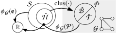
Figure 9: The relations between sets and functions in Section 6.

Lemma 18.

Given a connected graph $\mathcal{G}$ and its associated star function $\phi_{\mathcal{G}}$, if $\phi_{\mathcal{G}}\leq 0$ on all of the bipartitions of $\mathcal{G}$, then $\phi_{\mathcal{G}}\leq 0$ on all of the tripartitions of $\mathcal{G}$.

The proof is composed of three steps. First, we determine what conditions must hold so that $\phi_{\mathcal{G}}(\mathcal{B})\leq 0$ for any bipartition $\mathcal{B}$. Then, we do the same for a generic tripartition $\mathcal{T}$. Finally, we show that, for each $\mathcal{T}$, there exists a specific $\mathcal{B}^{\prime}$ such that $\phi_{\mathcal{G}}(\mathcal{B}^{\prime})\leq 0\Rightarrow\phi_{\mathcal{G}}(\mathcal{T})\leq 0$. Hence, if $\phi_{\mathcal{G}}(\mathcal{B})\leq 0$ for all $\mathcal{B}\in\hat{\mathcal{B}}$, then also $\phi_{\mathcal{G}}(\mathcal{T})\leq 0$ for all $\mathcal{T}\in\hat{\mathcal{T}}$, that is the thesis.

(i)  Let us consider a generic bipartition $\mathcal{B}=\{\mathcal{I}_{1},\mathcal{I}_{2}\}$ of $\mathcal{G}$. Then, from (5) and (7), we can write

$$\phi_{\mathcal{G}}(\mathcal{B})=a_{1}(N_{1}\left\lvert\epsilon_{1}\right\rvert+N_{2}\left\lvert\epsilon_{2}\right\rvert)-a_{2}b\left\lvert\epsilon_{1}-\epsilon_{2}\right\rvert,$$ (9)

where $N_{1}=\left\lvert\mathcal{I}_{1}\right\rvert$, $N_{2}=\left\lvert\mathcal{I}_{2}\right\rvert$, $b$ is the number of edges connecting vertices in $\mathcal{I}_{1}$ with vertices in $\mathcal{I}_{2}$ (see Figure 7), and $\epsilon_{1},\epsilon_{2}$ are (different non-zero) constants depending on the generic vector $\hat{\mathbf{e}}\in\mathcal{S}$ whose clusterization corresponds to $\mathcal{B}$ according to (7). Even though $N_{1}$, $N_{2}$, and $b$ depend on the specific $\mathcal{B}$ being considered, we omit this dependence to simplify the notation. Since $\sum_{i=1}^{N}\hat{e}_{i}=0$, then $N_{1}\epsilon_{1}+N_{2}\epsilon_{2}=0$, that is $\epsilon_{2}=-\frac{N_{1}}{N_{2}}\epsilon_{1}$. Therefore, we may rewrite $\phi_{\mathcal{G}}(\mathcal{B})=2a_{1}N_{1}\left\lvert\epsilon_{1}\right\rvert-a_{2}b\tfrac{N_{1}+N_{2}}{N_{2}}\left\lvert\epsilon_{1}\right\rvert$. Hence, $\phi_{\mathcal{G}}(\mathcal{B})\leq 0$ if and only if

$$a_{2}\geq\frac{2a_{1}N_{1}N_{2}}{(N_{1}+N_{2})b},$$ (10)

independently from the value of the constants $\epsilon_{1}$ and $\epsilon_{2}$ associated to the specific vector whose clusterization is being considered.

(ii)  Let us now consider a generic tripartition $\mathcal{T}=\{\mathcal{I}_{1},\mathcal{I}_{2},\mathcal{I}_{3}\}$. Using similar arguments to those presented for bipartitions, from (5) and (8), we obtain

$$\phi_{\mathcal{G}}(\mathcal{T})=a_{1}(N_{1}\left\lvert\epsilon_{1}\right\rvert+N_{2}\left\lvert\epsilon_{2}\right\rvert+N_{3}\left\lvert 0\right\rvert)\\ -a_{2}(b\left\lvert\epsilon_{1}-\epsilon_{2}\right\rvert+l_{1}\left\lvert\epsilon_{1}-0\right\rvert+l_{2}\left\lvert\epsilon_{2}-0\right\rvert),$$ (11)

where $N_{1}=\left\lvert\mathcal{I}_{1}\right\rvert$, $N_{2}=\left\lvert\mathcal{I}_{2}\right\rvert$, $N_{3}=\left\lvert\mathcal{I}_{3}\right\rvert$, and $b$, $l_{1}$, $l_{2}$ are the numbers of edges connecting vertices in $\mathcal{I}_{1}$ with vertices in $\mathcal{I}_{2}$, vertices in $\mathcal{I}_{1}$ with vertices in $\mathcal{I}_{3}$, and vertices in $\mathcal{I}_{2}$ with vertices in $\mathcal{I}_{3}$, respectively (see Figure 8). $N_{1}$, $N_{2}$, $N_{3}$, $b$, $l_{1}$, and $l_{2}$ all depend on $\mathcal{T}$. Since $\sum_{i=1}^{N}\hat{e}_{i}=0$, then $N_{1}\epsilon_{1}+N_{2}\epsilon_{2}+N_{3}\cdot 0=0$, that is again $\epsilon_{2}=-\frac{N_{1}}{N_{2}}\epsilon_{1}$. In view of this, and multiplying both sides of (11) by $N_{2}$, we obtain $N_{2}\phi_{\mathcal{G}}(\mathcal{T})=2a_{1}N_{1}N_{2}\left\lvert\epsilon_{1}\right\rvert-a_{2}(b(N_{1}+N_{2})\left\lvert\epsilon_{1}\right\rvert+l_{1}N_{2}\left\lvert\epsilon_{1}\right\rvert+l_{2}N_{1}\left\lvert\epsilon_{2}\right\rvert)$. As $N_{2}>0$, this yields that $\phi_{\mathcal{G}}(\mathcal{T})\leq 0$ if and only if

$$a_{2}\geq\frac{2a_{1}N_{1}N_{2}}{b(N_{1}+N_{2})+N_{2}l_{1}+N_{1}l_{2}}.$$ (12)

(iii)  We now show that

$$\forall\mathcal{T}\in\hat{\mathcal{T}}\ \exists\mathcal{B}^{\prime}\in\hat{\mathcal{B}}\ \text{s.t.}\ \phi_{\mathcal{G}}(\mathcal{B}^{\prime})\leq 0\Rightarrow\phi_{\mathcal{G}}(\mathcal{T})\leq 0.$$ (13)

Let us consider again the generic tripartition $\mathcal{T}=\{\mathcal{I}_{1},\mathcal{I}_{2},\mathcal{I}_{3}\}$ introduced in point (ii); see Figure 8 for a graphical representation. With an appropriate labelling of the clusters, without loss of generality we can assume that $l_{2}\geq l_{1}$. To any $\mathcal{T}$, we can always associate a specific bipartition $\mathcal{B}^{\prime}=\{\mathcal{I}_{1}^{\prime},\mathcal{I}_{2}^{\prime}\}$, where $\mathcal{I}_{1}^{\prime}=\mathcal{I}_{1}$ and $\mathcal{I}_{2}^{\prime}=\mathcal{I}_{2}\cup\mathcal{I}_{3}$, characterised by $N_{1}^{\prime}=\left\lvert\mathcal{I}_{1}^{\prime}\right\rvert$, $N_{2}^{\prime}=\left\lvert\mathcal{I}_{2}^{\prime}\right\rvert$, and $b^{\prime}$ being the number of edges between $\mathcal{I}_{1}^{\prime}$ and $\mathcal{I}_{2}^{\prime}$. Thus, it follows that $N_{1}^{\prime}=N_{1}$, $N_{2}^{\prime}=N_{2}+N_{3}$, and $b^{\prime}=b+l_{1}$. According to (10), $\phi_{\mathcal{G}}(\mathcal{B}^{\prime})\leq 0$ if and only if

$$a_{2}\geq\frac{2a_{1}N_{1}^{\prime}N_{2}^{\prime}}{(N_{1}^{\prime}+N_{2}^{\prime})b^{\prime}}=\frac{2a_{1}N_{1}(N_{2}+N_{3})}{(N_{1}+N_{2}+N_{3})(b+l_{1})}.$$ (14)

Next, we prove that (14) implies (12), independently of $\mathcal{T}$. To that aim, we need to show that

$$\frac{2N_{1}(N_{2}+N_{3})}{(N_{1}+N_{2}+N_{3})(b+l_{1})}\geq\frac{2N_{1}N_{2}}{b(N_{1}+N_{2})+N_{2}l_{1}+N_{1}l_{2}},$$

which is trivially verified by recalling that $l_{2}\geq l_{1}$. The thesis directly follows. ∎

We are now ready to give the final result that summarises previous findings and will be used in the proof of the main theorem.

Lemma 19.

If $\phi_{\mathcal{G}}\leq 0$ on all the bipartitions of $\mathcal{G}$, then $\phi_{\mathcal{G}}\leq 0$ for all $\mathbf{e}\in\mathcal{S}$.

According to Lemma 18, since $\phi_{\mathcal{G}}(\mathcal{B})\leq 0$ for all $\mathcal{B}\in\hat{\mathcal{B}}$, then

$$\phi_{\mathcal{G}}(\mathcal{P})\leq 0,\quad\forall\ \mathcal{P}\in\hat{\mathcal{P}}.$$ (15)

Exploiting Lemma 17, the clusterization $\mathrm{clus}(\hat{\mathbf{e}})$ of each generator $\hat{\mathbf{e}}\in\hat{\mathcal{H}}$ is a partition $\mathcal{P}\in\hat{\mathcal{P}}$. Therefore, (15) implies that

$$\phi_{\mathcal{G}}(\hat{\mathbf{e}})\leq 0,\quad\forall\ \hat{\mathbf{e}}\in\hat{\mathcal{H}}.$$ (16)

Recalling that $\phi_{\mathcal{G}}$ is a star function, (16) implies the thesis through Lemma 16. ∎

6.4 Proof of Theorem 6

The dynamics of the average state $\tilde{\mathbf{x}}$ of network (1) under the multilayer control action (2) are given by $\dot{\tilde{\mathbf{x}}}=\frac{1}{N}\sum_{i=1}^{N}\mathbf{f}(\mathbf{x}_{i};t)$. Therefore, the synchronization error $\mathbf{e}_{i}$ evolves according to

$$\dot{\mathbf{e}}_{i}=\dot{\mathbf{x}}_{i}-\dot{\tilde{\mathbf{x}}}=\mathbf{f}(\mathbf{x}_{i};t)-\frac{1}{N}\sum_{i=1}^{N}\mathbf{f}(\mathbf{x}_{i};t)\\ -c\sum_{j=1}^{N}L_{ij}\bm{\Gamma}\mathbf{e}_{j}-c_{\mathrm{d}}\sum_{j=1}^{N}L_{ij}^{\mathrm{d}}\bm{\Gamma}_{\mathrm{d}}\mathrm{sign}(\mathbf{e}_{j}-\mathbf{e}_{i}),$$ (17)

where we used the fact that $\sum_{j=1}^{N}L_{ij}\left(\mathbf{x}_{j}-\mathbf{x}_{i}\right)=\sum_{j=1}^{N}L_{ij}\mathbf{x}_{j}=\sum_{j=1}^{N}L_{ij}\mathbf{e}_{j}$ and that $\mathrm{sign}(\mathbf{x}_{j}-\mathbf{x}_{i})=\mathrm{sign}(\mathbf{e}_{j}-\mathbf{e}_{i})$. Now, consider the candidate common Lyapunov function $V\triangleq\frac{1}{2}\sum_{i=1}^{N}\mathbf{e}_{i}^{\mathsf{T}}\mathbf{P}\mathbf{e}_{i}$. Its time derivative is $\dot{V}=\sum_{i=1}^{N}\mathbf{e}_{i}^{\mathsf{T}}\mathbf{P}\dot{\mathbf{e}}_{i}$, that is,

$$\dot{V}=\sum_{i=1}^{N}\mathbf{e}_{i}^{\mathsf{T}}\mathbf{P}\left(\mathbf{f}(\mathbf{x}_{i};t)-\frac{1}{N}\sum_{i=1}^{N}\mathbf{f}(\mathbf{x}_{i};t)\right)-c\sum_{i=1}^{N}\sum_{j=1}^{N}\\ L_{ij}\mathbf{e}_{i}^{\mathsf{T}}\mathbf{P}\bm{\Gamma}\mathbf{e}_{j}-c_{\mathrm{d}}\sum_{i=1}^{N}\sum_{j=1}^{N}L_{ij}^{\mathrm{d}}\mathbf{e}_{i}^{\mathsf{T}}\mathbf{P}\bm{\Gamma}_{\mathrm{d}}\mathrm{sign}(\mathbf{e}_{j}-\mathbf{e}_{i}).$$ (18)

As $\sum_{i=1}^{N}\mathbf{e}_{i}=0$, we have $\sum_{i=1}^{N}\mathbf{e}_{i}^{\mathsf{T}}\mathbf{P}\mathbf{f}(\tilde{\mathbf{x}};t)=0$ and $\sum_{i=1}^{N}\mathbf{e}_{i}^{\mathsf{T}}\mathbf{P}\left(\sum_{i=1}^{N}\mathbf{f}(\mathbf{x}_{i};t)/N\right)=0$. Thus, we can rewrite (18) as

$$\dot{V}=\sum_{i=1}^{N}\mathbf{e}_{i}^{\mathsf{T}}\mathbf{P}\left[\mathbf{f}(\mathbf{x}_{i};t)-\mathbf{f}(\tilde{\mathbf{x}};t)\right]-c\sum_{i=1}^{N}\sum_{j=1}^{N}L_{ij}\mathbf{e}_{i}^{\mathsf{T}}\mathbf{P}\bm{\Gamma}\mathbf{e}_{j}\\ -c_{\mathrm{d}}\sum_{(i,j)\in\mathcal{E}_{\mathrm{d}}}(\mathbf{e}_{i}-\mathbf{e}_{j})^{\mathsf{T}}\mathbf{P}\bm{\Gamma}_{\mathrm{d}}\mathrm{sign}(\mathbf{e}_{i}-\mathbf{e}_{j}),$$ (19)

where we also exploited that, since $L_{ij}^{\mathrm{d}}=L_{ji}^{\mathrm{d}}$, for each term $\mathbf{e}_{i}^{\mathsf{T}}\mathbf{P}\bm{\Gamma}_{\mathrm{d}}\mathrm{sign}(\mathbf{e}_{j}-\mathbf{e}_{i})$ there exists another term $\mathbf{e}_{j}^{\mathsf{T}}\mathbf{P}\bm{\Gamma}_{\mathrm{d}}\mathrm{sign}(\mathbf{e}_{i}-\mathbf{e}_{j})$; in addition, we recall that $\mathcal{E}_{\mathrm{d}}$ is the set of edges in the graph $\mathcal{G}_{\mathrm{d}}$. Then, we use the hypothesis that $\mathbf{f}$ is -QUAD and get

$$\dot{V}\leq\sum_{i=1}^{N}\left(\mathbf{e}_{i}^{\mathsf{T}}\mathbf{Q}\mathbf{e}_{i}+\mathbf{e}_{i}^{\mathsf{T}}\mathbf{M}\mathrm{sign}(\mathbf{e}_{i})\right)-c\sum_{i=1}^{N}\sum_{j=1}^{N}L_{ij}\\ \mathbf{e}_{i}^{\mathsf{T}}\mathbf{P}\bm{\Gamma}\mathbf{e}_{j}-c_{\mathrm{d}}\sum_{(i,j)\in\mathcal{E}_{\mathrm{d}}}(\mathbf{e}_{i}-\mathbf{e}_{j})^{\mathsf{T}}\mathbf{P}\bm{\Gamma}_{\mathrm{d}}\mathrm{sign}(\mathbf{e}_{i}-\mathbf{e}_{j}).$$ (20)

Now, if we define $\bar{\mathbf{y}}\triangleq\left(\mathbf{B}_{\mathrm{d}}^{\mathsf{T}}\otimes\mathbf{I}_{n}\right)\bar{\mathbf{e}}$, where $\mathbf{B}_{\mathrm{d}}$ is the incidence matrix of $\mathcal{G}_{\mathrm{d}}$, then we can rewrite (20) as $\dot{V}\leq W_{1}+W_{2}$, where

$$W_{1}\triangleq\bar{\mathbf{e}}^{\mathsf{T}}\left(\mathbf{I}_{N}\otimes\mathbf{Q}-c\mathbf{L}\otimes\mathbf{P}\bm{\Gamma}\right)\bar{\mathbf{e}},$$ (21)

$$W_{2}\triangleq\bar{\mathbf{e}}^{\mathsf{T}}\left(\mathbf{I}_{N}\otimes\mathbf{M}\right)\mathrm{sign}(\bar{\mathbf{e}})-c_{\mathrm{d}}\bar{\mathbf{y}}{\color[rgb]{0,0,0}^{\mathsf{T}}}\left(\mathbf{I}_{\color[rgb]{0,0,0}N_{\mathcal{E}_{\mathrm{d}}}}\otimes\mathbf{P}\bm{\Gamma}_{\mathrm{d}}\right)\mathrm{sign}(\bar{\mathbf{y}}).$$ (22)

We can then study $W_{1}$ and $W_{2}$ separately, so as to find conditions that guarantee the former is negative definite and the latter is semi-negative definite.

6.4.1 Negativity of $W_{1}$

To find a condition such that $W_{1}<0$, note that $\lambda_{1}(\mathbf{L})=0$ with corresponding eigenvector $\mathbf{1}_{N}$ [21, § 13.1], and let $\mathbf{G}\triangleq\frac{\mathbf{P}\bm{\Gamma}+(\mathbf{P}\bm{\Gamma})^{\mathsf{T}}}{2}$. Then, by [22, Thm. 4.2.12], the first $n$ smallest eigenvalues of $\mathbf{L}\otimes\mathbf{G}$ are all 0, and the $n$ corresponding eigenvectors are $\mathbf{1}_{N}\otimes\mathbf{w}_{i}$, where $\mathbf{w}_{i}$, $i=1,\dots,n$ are the eigenvectors of $\mathbf{G}$. Notice that by construction $\bar{\mathbf{e}}$ is orthogonal to all these eigenvectors, as $\bar{\mathbf{e}}^{\mathsf{T}}(\mathbf{1}_{N}\otimes\mathbf{v})=0$ for any $\mathbf{v}\in\mathbb{R}^{n}$. Therefore, through [23, Thm. 4.2.2] we can write

$$\lambda_{n+1}\left(\mathbf{L}\otimes\mathbf{G}\right)=\min_{\bar{\mathbf{e}}:\,\bar{\mathbf{e}}^{\mathsf{T}}(\mathbf{1}_{N}\otimes\mathbf{v})=0,\,\bar{\mathbf{e}}\neq 0}\frac{\bar{\mathbf{e}}^{\mathsf{T}}\left(\mathbf{L}\otimes\mathbf{P}\bm{\Gamma}\right)\bar{\mathbf{e}}}{\bar{\mathbf{e}}^{\mathsf{T}}\bar{\mathbf{e}}}.$$

Hence, as $\lambda_{2}(\mathbf{L})\lambda_{1}\left(\mathbf{G}\right)=\lambda_{n+1}\left(\mathbf{L}\otimes\mathbf{G}\right)$, we get that $-c\bar{\mathbf{e}}^{\mathsf{T}}\left(\mathbf{L}\otimes\mathbf{P}\bm{\Gamma}\right)\bar{\mathbf{e}}\leq-c\lambda_{2}(\mathbf{L})\mu_{2}^{-}(\mathbf{P}\bm{\Gamma})\left\lVert\bar{\mathbf{e}}\right\rVert_{2}^{2}$. Moreover, it holds that $\bar{\mathbf{e}}^{\mathsf{T}}\left(\mathbf{I}_{N}\otimes\mathbf{Q}\right)\bar{\mathbf{e}}\leq\left\lVert\bar{\mathbf{e}}\right\rVert_{2}^{2}\lambda_{\mathrm{max}}(\frac{\mathbf{Q}+\mathbf{Q}^{\mathsf{T}}}{2})$. Thus, in (21), $W_{1}<0$ if $c>c^{*}$, with $c^{*}$ defined as in (4). Note that the fact that $\mathcal{G}$ is connected ensures that $\lambda_{2}(\mathbf{L})>0$.

6.4.2 Semi-negativity of $W_{2}$

Next, we seek an expression of the threshold value $c_{\mathrm{d}}^{*}$ such that $W_{2}\leq 0$ if $c_{\mathrm{d}}\geq c_{\mathrm{d}}^{*}$. Firstly, consider that, from (22), using Lemmas 9 and 10, we have

$$W_{2}\leq\left\lVert\bar{\mathbf{e}}\right\rVert_{1}{\color[rgb]{0,0,0}\mu_{\infty}(\mathbf{M})}-c_{\mathrm{d}}\left\lVert\bar{\mathbf{y}}\right\rVert_{1}\mu_{\infty}^{-}(\mathbf{P}\bm{\Gamma}_{\mathrm{d}}).$$ (23)

Using the definition of the vector 1-norm, we have $\lVert\bar{\mathbf{e}}\rVert_{1}=\sum_{i=1}^{nN}\lvert\bar{e}_{i}\rvert=\sum_{h=1}^{n}\lVert\mathbf{e}^{h}\rVert_{1}=\sum_{h=1}^{n}\sum_{i=1}^{N}\lvert\mathbf{i}_{i}^{\mathsf{T}}\mathbf{e}^{h}\rvert$, where $\mathbf{i}_{i}$ and $\mathbf{e}^{h}$ are defined in Section 3. Note that $\mathbf{e}^{h}\in\mathcal{S}$, with $\mathcal{S}$ being defined in Section 6.3. Similarly, it is straightforward to compute that $\left\lVert\bar{\mathbf{y}}\right\rVert_{1}=\sum_{h=1}^{n}\sum_{i=1}^{N_{\mathcal{E}_{\mathrm{d}}}}\left\lvert\mathbf{b}_{i}^{\mathsf{T}}\mathbf{e}^{h}\right\rvert$, where $\mathbf{b}_{i}$ are the columns of the incidence matrix $\mathbf{B}_{\mathrm{d}}$ of $\mathcal{G}_{\mathrm{d}}$. For the sake of compactness, we define $M\triangleq{\color[rgb]{0,0,0}\mu_{\infty}(\mathbf{M})}$ and ${\color[rgb]{0,0,0}\gamma}\triangleq\mu_{\infty}^{-}(\mathbf{P}\bm{\Gamma}_{\mathrm{d}})$. Thus, we can recast (23) as $W_{2}\leq\sum_{h=1}^{n}W_{2}^{h}$, where

$$W_{2}^{h}(\mathbf{e}^{h})\triangleq M\sum_{i=1}^{N}\left\lvert\mathbf{i}_{i}^{\mathsf{T}}\mathbf{e}^{h}\right\rvert-c_{\mathrm{d}}{\color[rgb]{0,0,0}\gamma}\sum_{i=1}^{N_{\mathcal{E}_{\mathrm{d}}}}\left\lvert\mathbf{b}_{i}^{\mathsf{T}}\mathbf{e}^{h}\right\rvert.$$ (24)

The analytical framework and results presented in Sections 6.2 and 6.3 can be used to more easily assess the semi-negativity of $W_{2}^{h}$. In fact, $W_{2}^{h}$ is in the form (5), and thus is a star function associated to the graph $\mathcal{G}_{\mathrm{d}}$; see Definition 15. Exploiting Lemma 19, it is immediate to state that $W_{2}^{h}(\mathbf{e}^{h})\leq 0$ for all $\mathbf{e}^{h}\in\mathcal{S}$ (that is, globally) if $W_{2}^{h}(\mathcal{B})\leq 0$ for all $\mathcal{B}\in\hat{\mathcal{B}}$; $\hat{\mathcal{B}}$ being the set of all bipartitions of $\mathcal{G}_{\mathrm{d}}$.

Consider a generic bipartition $\mathcal{B}=\{\mathcal{I}_{1},\mathcal{I}_{2}\}$ of $\mathcal{G}_{\mathrm{d}}$, where $\mathcal{I}_{1}$ and $\mathcal{I}_{2}$ are the indices of the vertices in the two connected clusters. Moreover, let $N_{1}=\left\lvert\mathcal{I}_{1}\right\rvert$, $N_{2}=\left\lvert\mathcal{I}_{2}\right\rvert$, and $b$ be the number of edges connecting a vertex in $\mathcal{I}_{1}$ with a vertex in $\mathcal{I}_{2}$ (see Figure 7); note that $N_{1}$, $N_{2}$, and $b$ depend on $\mathcal{B}$. According to (9) and (10), $W_{2}^{h}(\mathcal{B})\leq 0$ if and only if

$$c_{\mathrm{d}}\geq\frac{2M}{N{\color[rgb]{0,0,0}\gamma}}\left(\frac{N_{1}N_{2}}{b}\right),$$ (25)

where we used the fact that $N_{1}+N_{2}=N$. We highlight that this last step is independent from $h$; therefore, if (25) holds, then $W_{2}^{h}(\mathcal{B})\leq 0\ \forall h=1,\dots,n$. From the hypotheses we know that

$$c_{\mathrm{d}}\geq c_{\mathrm{d}}^{*}\triangleq\frac{1}{\delta_{\mathcal{G}_{\mathrm{d}}}}\frac{M}{{\color[rgb]{0,0,0}\gamma}}=\frac{2M}{N{\color[rgb]{0,0,0}\gamma}}\frac{1}{\min_{\mathcal{C}\in\hat{\mathcal{C}}_{\mathcal{G}_{\mathrm{d}}}}\left(\frac{b}{N_{1}N_{2}}\right)}.$$ (26)

where $\delta_{\mathcal{G}_{\mathrm{d}}}$ is the minimum density of $\mathcal{G}_{\mathrm{d}}$ (Definition 5) and $\hat{\mathcal{C}}_{\mathcal{G}_{\mathrm{d}}}$ is the set of all possible cuts on $\mathcal{G}_{\mathrm{d}}$. Thus, (26) can be reformulated as

$$c_{\mathrm{d}}\geq\frac{2M}{N{\color[rgb]{0,0,0}\gamma}}\frac{1}{\min_{\mathcal{B}\in\hat{\mathcal{B}}}\left(\frac{b}{N_{1}N_{2}}\right)}=\frac{2M}{N{\color[rgb]{0,0,0}\gamma}}\max_{\mathcal{B}\in\hat{\mathcal{B}}}\left(\frac{N_{1}N_{2}}{b}\right).$$ (27)

Therefore, (25) holds for all $\mathcal{B}\in\hat{\mathcal{B}}$. This ensures that $W_{2}^{h}(\mathcal{B})\leq 0$ for all $\mathcal{B}\in\hat{\mathcal{B}}$, which through Lemma 19 gives $W_{2}^{h}\leq 0$ globally. As mentioned previously, if $W_{2}^{h}\leq 0$ for some $h$, then $W_{2}^{h}\leq 0$ for all $h$, and hence $W_{2}\leq 0$. This completes the proof, as $\dot{V}=W_{1}+W_{2}<0$ globally. ∎

We note that the occurrence of sliding dynamics does not impact the analysis, which is conducted using a common Lyapunov function method, with $V$ being a valid Lyapunov function in all the state space of the network, even in the regions where there is sliding (if any).

7 Conclusions

We addressed the challenging problem of proving global asymptotic convergence to synchronization in a network of piecewise-smooth dynamical systems, without employing, as done in previous attempts in the literature, costly centralised control actions on all the nodes. We showed that, under some assumptions on the agents’ vector field, adding a discontinuous coupling layer to the commonly used diffusive coupling protocol is sufficient to ensure convergence.

We derived sufficient conditions that allow computation of the critical values of the coupling gains required for convergence. The conditions depend explicitly on structural properties of the underlying network graphs that can be computed algorithmically. In particular, we introduced the concept of minimum density of a graph that can be used to compute the critical coupling gain of the discontinuous control layer.

An open problem left for further study is to investigate if there exist some best structures of the diffusive and discontinuous coupling layers in terms of performance, robustness and stability. For example, preliminary numerical simulations reported in [9] show that different layers’ structures can enhance the regions in the control parameter space where synchronization is attained.

The authors sincerely thank Josep M. Olm (Universitat Politècnica de Catalunya) for his insightful comments and suggestions during the preparation of this manuscript.

References

- [1] Alex Arenas, Albert Díaz-Guilera, Jürgen Kurths, Yamir Moreno, and Changsong Zhou. Synchronization in complex networks. Physics Reports, 469(3):93–153, 2008.
- [2] Sanjeev Arora, Elad Hazan, and Satyen Kale. approximation to sparsest cut in time. SIAM Journal on Computing, 39(5):1748–1771, 2010.
- [3] Winfried Bruns and Joseph Gubeladze. Polytopes, Rings, and K-Theory. Springer, 2009.
- [4] Daniel Alberto Burbano Lombana and Mario di Bernardo. Multiplex PI control for consensus in networks of heterogeneous linear agents. Automatica, 67:310–320, 2016.
- [5] R. Burridge and L. Knopoff. Model and theoretical seismicity. Bulletin of the Seismological Society of America, 57(3):341–371, 1967.
- [6] Richard Casey, Hidde de Jong, Jean-Luc Luc Gouzé, Hidde De Jong, and Jean-Luc Luc Gouzé. Piecewise-linear models of genetic regulatory networks: Equilibria and their stability. Journal of Mathematical Biology, 52(1):27–56, 2006.
- [7] Stephen Coombes, Yi Ming Lai, Mustafa Şayli, and Rüdiger Thul. Networks of piecewise linear neural mass models. European Journal of Applied Mathematics, 29(5):869–890, 2018.
- [8] Stephen Coombes and Rüdiger Thul. Synchrony in networks of coupled non-smooth dynamical systems: Extending the master stability function. European Journal of Applied Mathematics, 27(06):904–922, 2016.
- [9] Marco Coraggio, Pietro De Lellis, S. John Hogan, and Mario di Bernardo. Synchronization of networks of piecewise-smooth systems. IEEE Control Systems Letters, 2(4):653–658, 2018.
- [10] Marco Coraggio, Pietro DeLellis, and Mario di Bernardo. Distributed discontinuous coupling for convergence in networks of heterogeneous nonlinear systems. arXiv:2003.10348, 2020.
- [11] Jorge Cortés. Finite-time convergent gradient flows with applications to network consensus. Automatica, 42(11):1993–2000, 2006.
- [12] Jorge Cortés. Discontinuous dynamical systems. IEEE Control Systems Magazine, 28(3):36–73, 2008.
- [13] Marius F. Danca. Synchronization of switch dynamical systems. International Journal of Bifurcation and Chaos, 12(08):1813–1826, 2002.
- [14] Pietro DeLellis, Mario di Bernardo, and Davide Liuzza. Convergence and synchronization in heterogeneous networks of smooth and piecewise smooth systems. Automatica, 56:1–11, 2015.
- [15] Pietro DeLellis, Mario di Bernardo, and Giovanni Russo. On QUAD, Lipschitz, and contracting vector fields for consensus and synchronization of networks. IEEE Transactions on Circuits and Systems I: Regular Papers, 58(3):576–583, 2011.
- [16] Mario di Bernardo, Chris Budd, Alan Richard Champneys, and Piotr Kowalczyk. Piecewise-Smooth Dynamical Systems: Theory and Applications. Springer, 2008.
- [17] Florian Dorfler, John W. Simpson-Porco, and Francesco Bullo. Breaking the hierarchy: Distributed control and economic optimality in microgrids. IEEE Transactions on Control of Network Systems, 3(3):241–253, 2016.
- [18] Andreas K. Engel, Pascal Fries, Peter König, Michael Brecht, and Wolf Singer. Temporal binding, binocular rivalry, and consciousness. Consciousness and Cognition, 8(2):128–151, 1999.
- [19] Miroslav Fiedler. Absolute algebraic connectivity of trees. Linear and Multilinear Algebra, 26(1-2):85–106, 1990.
- [20] Ugo Galvanetto. Non-linear dynamics of multiple friction oscillators. Computer Methods in Applied Mechanics and Engineering, 178(3-4):291–306, 1999.
- [21] Chris Godsil and Gordon F Royle. Algebraic Graph Theory. Springer, 2013.
- [22] Roger A. Horn and Charles R. Johnson. Topics in Matrix Analysis. Cambridge University Press, first edition, 1991.
- [23] Roger A. Horn and Charles R. Johnson. Matrix Analysis. Cambridge University Press, 2nd ed edition, 2012.
- [24] Qing Hui, Wassim M. Haddad, and Sanjay P. Bhat. Finite-time semistability, Filippov systems, and consensus protocols for nonlinear dynamical networks with switching topologies. Nonlinear Analysis: Hybrid Systems, 4(3):557–573, 2010.
- [25] George Karypis and Vipin Kumar. A fast and high quality multilevel scheme for partitioning irregular graphs. SIAM Journal on Scientific Computing, 20(1):359–392, 1998.
- [26] Yi Ming Lai, Rüdiger Thul, and Stephen Coombes. Analysis of networks where discontinuities and nonsmooth dynamics collide: Understanding synchrony. European Physical Journal: Special Topics, 227(10-11):1251–1265, 2018.
- [27] Remco I. Leine and H. Nijmeijer. Dynamics and Bifurcations of Non-Smooth Mechanical Systems. Springer, 2004.
- [28] Daniel Liberzon. Switching in Systems and Control. Birkhäuser, 2012.
- [29] Bo Liu, Wenlian Lu, and Tianping Chen. New conditions on synchronization of networks of linearly coupled dynamical systems with non-Lipschitz right-hand sides. Neural Networks, 25(200921):5–13, 2012.
- [30] Xiaoyang Liu, Jinde Cao, and Wenwu Yu. Filippov systems and quasi-synchronization control for switched networks. Chaos, 22(3), 2012.
- [31] Xiaoyang Liu, Tianping Chen, Jinde Cao, and Wenlian Lu. Dissipativity and quasi-synchronization for neural networks with discontinuous activations and parameter mismatches. Neural Networks, 24(10):1013–1021, 2011.
- [32] David W. Matula and Farhad Shahrokhi. Sparsest cuts and bottlenecks in graphs. Discrete Applied Mathematics, 27(1-2):113–123, 1990.
- [33] Christopher G. Mayhew, Ricardo G. Sanfelice, Jansen Sheng, Murat Arcak, and Andrew R. Teel. Quaternion-based hybrid feedback for robust global attitude synchronization. IEEE Transactions on Automatic Control, 57(8):2122–2127, 2012.
- [34] Louis M. Pecora and Thomas L. Carroll. Master stability functions for synchronized coupled systems. Physical Review Letters, 80(10):2109–2112, 1998.
- [35] Christopher H. Scholz. Large earthquake triggering, clustering, and the synchronization of faults. Bulletin of the Seismological Society of America, 100(3):901–909, 2010.
- [36] Chi Kong Tse. Complex Behavior of Switching Power Converters. CRC Press, 2004.
- [37] Iakov Z. Tsypkin. Relay control systems. Cambridge University Press, 1984.
- [38] Jieqiang Wei, Silun Zhang, Antonio Adaldo, Johan Thunberg, Xiaoming Hu, and Karl Henrik Johansson. Finite-time attitude synchronization with distributed discontinuous protocols. IEEE Transactions on Automatic Control, 63(10):3608–3615, 2018.
- [39] P. Yang, R. A. Freeman, G. J. Gordon, K. M. Lynch, S. S. Srinivasa, and R. Sukthankar. Decentralized estimation and control of graph connectivity for mobile sensor networks. Automatica, 46(2):390–396, 2010.
- [40] Xinsong Yang, Zhiyou Wu, and Jinde Cao. Finite-time synchronization of complex networks with nonidentical discontinuous nodes. Nonlinear Dynamics, 73(4):2313–2327, 2013.