Synchronization to big-data:
nudging the Navier-Stokes equations for data assimilation of turbulent flows

Abstract

Nudging is an important data assimilation technique where partial field measurements are used to control the evolution of a dynamical system and/or to reconstruct the entire phase-space configuration of the supplied flow. Here, we apply it to the toughest problem in fluid dynamics: three dimensional homogeneous and isotropic turbulence. By doing numerical experiments we perform a systematic assessment of how well the technique reconstructs large- and small-scales features of the flow with respect to the quantity and the quality/type of data supplied to it. The types of data used are: (i) field values on a fixed number of spatial locations (Eulerian nudging), (ii) Fourier coefficients of the fields on a fixed range of wavenumbers (Fourier nudging), or (iii) field values along a set of moving probes inside the flow (Lagrangian nudging). We present state-of-the-art quantitative measurements of the scale-by-scale transition to synchronization and a detailed discussion of the probability distribution function of the reconstruction error, by comparing the nudged field and the truth point-by-point. Furthermore, we show that for more complex flow configurations, like the case of anisotropic rotating turbulence, the presence of cyclonic and anticyclonic structures leads to unexpectedly better performances of the algorithm. We discuss potential further applications of nudging to a series of applied flow configurations, including the problem of field-reconstruction in thermal Rayleigh-Bénard convection and in magnetohydrodynamics (MHD), and to the determination of optimal parametrisation for small-scale turbulent modeling. Our study fixes the standard requirements for future applications of nudging to complex turbulent flows.

I Introduction

Turbulence is the chaotic, non-linear, and multiscale motion observed in fluids. From astro- and geo-physical flows to engineering ones, it is a problem that surrounds us all Davidson (2013); Pope (2000). Thus, observing, measuring, reconstructing, and then predicting the evolution of turbulent flows are highly important tasks with direct consequences to our day to day lives. A paradigmatic example is given by the problem of state estimation in geo-sciences, of particular importance to numerical weather prediction (NWP) Kalnay (2003). The chaotic and multiscale nature of turbulence makes these tasks very difficult, as any small error in the initial conditions will make predictions diverge from the truth and as it is not easy to access all active modes in a fluid flow. This is particularly troublesome when one considers that in a turbulent flow the number of active degrees of freedom (dof) grows with the Reynolds number as $\#_{dof}\propto Re^{9/4}$, with $Re=UL/\nu$, given in terms of the typical rms velocity $U$, the energy containing scale $L$ and the fluid viscosity, $\nu$. Data assimilation (DA) is the family of mathematical protocols used to reconstruct the initial state of a dynamical system, out of a series of previous partial measurements, in order to ensure that any future predictions will be as faithful as possible to what the actual physical reality will be, and has proven to be of key importance in the development of modern NWP Bannister R. N. (2016); Carrassi et al. (2018); Bauer et al. (2015).

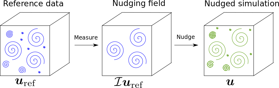
Figure 1: Diagram outlining the nudging algorithm. In our numerical experiments the reference data comes from a well controlled direct numerical simulation, and the process of measuring is summarized by the filtering operation $\mathcal{I}$.

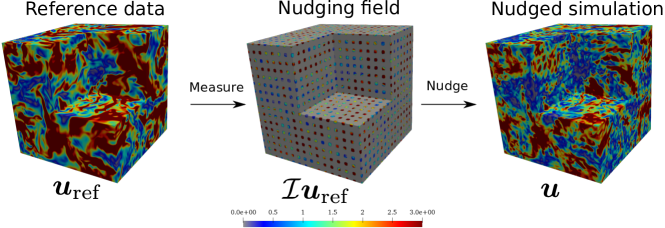
Figure 2: First row: visualizations of (left) reference fields ${\bm{u}}_{\rm ref}$, (middle) filtered/nudging fields $\mathcal{I}{\bm{u}}_{\rm ref}$, and (right) nudged/reconstructed fields ${\bm{u}}$ for Eulerian nudging. The parameters are $\alpha t_{\eta}=0.40$, $\tau/t_{\eta}=25$, $\phi=0.05$. Second row the same of above but for Lagrangian nudging. The parameters are $\alpha t_{\eta}=0.40$, $\tau/t_{\eta}=25$, $\phi=0.03$.

Given the problem of trying to reconstruct the whole flow configuration out of some partial data, one may ask two crucial questions. The first one is about the quantity of information that one needs to collect in order to achieve a certain degree of reconstruction. The second one concerns how the quality, or type, of information affects the level of reconstruction that can be attained. The two main tools used in DA are based on either variational or ensemble-averaged approaches. Variational methods, best exemplified by the 4D-Var technique Talagrand and Courtier (1987); Park and Županski (2003); Rawlins et al. (2007), rely on minimizing the distance between a simulated system’s trajectory with the available data. In order to do this, the statistics of the errors are assumed to be Gaussian. Ensemble approaches work by performing Kalman filtering operations Evensen (1994, 2006); Houtekamer and Zhang (2016) on the probability distributions of different realizations of the state to be reconstructed. Similarly to the variational approaches, they also assume the statistics to be Gaussian. Both techniques have proven useful in NWP and have also been applied to mildly turbulent channel flows Bewley and Protas (2004); Suzuki (2012); Suzuki and Hasegawa (2017), but they have never been put to these in fully-developed turbulence, where the small-scale velocity statistics is intermittent with fat and non-Gaussian tails, and the system is strongly out of equilibrium. This constitutes a big hurdle to overcome also for NWP, as new technological developments in computational and measuring tools allow weather forecast centers to reach resolutions where three-dimensional turbulent convection becomes important Leutwyler et al. (2016); Yano et al. (2018), signaling we are entering an era where non-linear DA schemes have to be put to use. One possible scheme is Particle Filtering Gordon et al. (1993), which works like the Kalman filter based approaches but without employing the Gaussianity assumption. This scheme has already been put to test in two-dimensional barotropic flows van Leeuwen and Ades (2013) and weather models Poterjoy et al. (2017), showing better results than linear DA schemes, but still presenting non-trivial obstacles when scaling to high-dimensional systems.

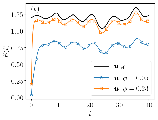
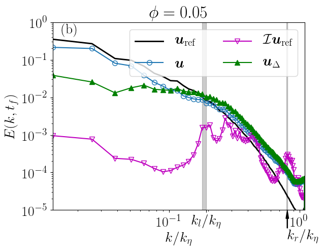
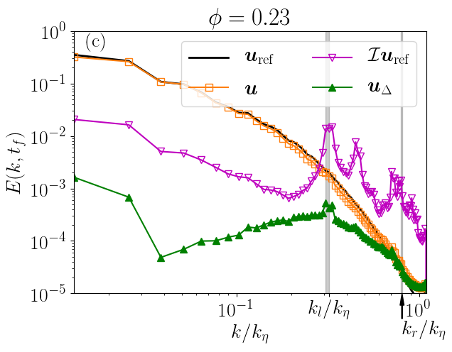
Figure 3: (a) Evolution of the total energy for the reference field and for two nudged fields with different volume fraction, before and close to full synchronization, $\phi=0.05,0.23$. Log-log plots of (b) the energy spectra for the reference field (the truth), ${\bm{u}}_{\rm ref}$), the nudging partial data, ${\cal I}{\bm{u}}_{\rm ref}$ and the nudged/reconstructed field on the whole volume ${\bm{u}}$. We also plot the spectrum of the error field, ${\bm{u}}_{\Delta}$. with $\phi=0.05$ and (c) for $\phi=0.23$. Grey regions mark the two typical wavenumbers $k_{l}$ and $k_{r}$ (see text). Notice the transition to full synchronization for panel (c) where the spectrum of the error field, ${\bm{u}}_{\Delta}$, is negligible at all scales.

In this paper, we propose to use nudging Hoke and Anthes (1976); Lakshmivarahan and Lewis (2013); Clark Di Leoni et al. (2018), a fully unbiased approach, to numerically study the problem of assimilating data into a turbulent flow which is characterized by a high (infinite) dimensional phase-space with strong non-Gaussian and intermittent multi-scale fluctuations Frisch (1995); Pope (2000). Nudging has an old and prestigious past in DA history Hoke and Anthes (1976); Lakshmivarahan and Lewis (2013). It consists of applying a penalty term to the right hand side of the evolution equations that tries to minimize the distance between the evolved flow and the observations (see Fig. 1 for a sketch). In a way, nudging can be viewed as the application of a Newton relaxation feedback to fluid flows. In the context of NWP, different formulations of nudging have been used to study the state estimation problem using finite dimensional dynamical systems and weather models Hoke and Anthes (1976); Auroux and Blum (2008); Du and Smith (2013); Pazó et al. (2016), and for boundary condition matching von Storch et al. (2000); Waldron et al. (1996); Miguez-Macho et al. (2004). In the context of turbulence, for the cases of two-dimensional Navier-Stokes Equation Farhat et al. (2016); Gesho et al. (2016); Foias et al. (2016); Biswas et al. (2017), the three-dimensional Navier-Stokes $\alpha$ model Albanez et al. (2016), and Rayleigh-Bernard convection Farhat et al. (2017, 2019), it has been rigorously proven that given a sufficient amount of input data a nudged field will eventually synchronize with its nudging field. Indeed, both DA Carrassi et al. (2008) and nudging can be framed as a synchronization problem, see Lalescu et al. (2013) for an application similar to Fourier nudging for turbulence.

Before moving on, we should note that in the current data-driven age, parameter reconstruction is another key problem for accurate flow prediction, modelling, and control. Here the goal is to recover, out of some given data, the form and/or the parameters of the underlying PDEs (or ODEs) that generated such data. Modern methods include (but are not restricted to) symbolic regression coupled with sparsity methods Brunton et al. (2016); Rudy et al. (2017), physics informed neural networks Raissi et al. (2017a, b), statistical inference Cialenco and Glatt-Holtz (2011), and minimum ignorance approaches Du and Smith (2012). Recently, we have shown that nudging can be used to infer parameters and physics even for the case of three dimensional fully developed turbulence, both isotropic and under rotation Clark Di Leoni et al. (2018). Another related problem is the one of equation-free modelling, where recent advances haven been made in high dimensional systems by using reservoir computing techniques Pathak et al. (2018); Nakai and Saiki (2018), and in turbulent flows by using artificial neural networks Mohan et al. (2019). All these problems point to the pressing need of developing data-driven techniques that can be scaled to non-linear and high-dimensional problems such as turbulence.

Our novel goal is to present nudging as a tool to probe for the key degrees of freedom of a flow and understand where and what we need to measure to ensure a certain level of reconstruction. We tackle problems such as if it is better to (i) place the probes in a regular equispaced way, (ii) follow measurements in a Lagrangian domain, along floating probes, or (iii) perform first a Fourier convolution to spread the information on the whole configuration space. Furthermore, we will also study nudging in the presence of inverse energy cascade Alexakis and Biferale (2018) with the formation of highly coherent cyclonic/anticyclonic structures in rotating turbulence. These are the questions we will answer here, and that have not been addressed before. Many others will follow, that we leave for future research: What about bounded flows Kim et al. (1987); Hwang et al. (2016)? Is it better to place the probes close to the wall or in the bulk? What about multi-field equations as in Rayleigh-Bénard Fauve and Libchaber (1981); Ahlers et al. (2009) or MHD Léorat et al. (1981); Alexakis et al. (2005)? Can we control temperature by measuring velocity in convection? or velocity by measuring the magnetic field in MHD? All these questions have applied and fundamental importance.

The paper is organized as follows: in Sec. II we outline the how the nudging protocol works, in part II.1 we write down the equations, in II.2 we give details on the numerical implementations of the technique and of the simulations performed, and in II.3 we explain the different quantities we will use to measure the performance of nudging. We will then present the results of nudging in configuration space in III.1, of nudging in Fourier space in III.2, and of nudging under the presence or large scale structures in III.3. Finally, we present our conclusions in IV.

II Methods

II.1 Nudging the Navier-Stokes equations

Our application of Nudging is based on the following protocol. Suppose we have some measurements of a reference field data, ${\bm{u}}_{\rm ref}$, available only on certain regions of space (or for certain Fourier modes) and with a certain cadence in time, $\tau$. And suppose we know that the field evolution is described by the three dimensional incompressible Navier-Stokes equations (NSE) with unit density:

$$\begin{cases}\partial_{t}{\bm{u}}_{\rm ref}+{\bm{u}}_{\rm ref}\cdot{\bm{\nabla}}{\bm{u}}_{\rm ref}=-{\bm{\nabla}}p_{\rm ref}+\nu\nabla^{2}{\bm{u}}_{\rm ref}+\bm{f}_{\rm ref},\\ {\bm{\nabla}}\cdot{\bm{u}}_{\rm ref}=0,\\ +{\rm boundary\,conditions,}\end{cases}$$ (1)

where $\bm{f}_{\rm ref}$ is a forcing mechanism and $\nu$ the viscosity. The aim is to reconstruct the whole space-time evolution of ${\bm{u}}_{\rm ref}$ by evolving a numerical simulation for another incompressible velocity field ${\bm{u}}$, which we call the nudged field, where the distance from the input data ${\bm{u}}_{\rm ref}-{\bm{u}}$ enters as a penalty term:

$$\begin{cases}\partial_{t}{\bm{u}}+{\bm{u}}\cdot{\bm{\nabla}}{\bm{u}}=-{\bm{\nabla}}p+\nu\nabla^{2}{\bm{u}}-\alpha\mathcal{I}({\bm{u}}-{\bm{u}}_{\mathrm{ref}}),\\ {\bm{\nabla}}\cdot{\bm{u}}=0\\ +{\rm boundary\,conditions,}\end{cases}$$ (2)

where $\alpha$ is the amplitude of the nudging term, and $\mathcal{I}$ is a filtering operator which projects $\bm{u}-\bm{u}_{\rm ref}$ onto the regions of space (or the Fourier scales) in which the reference data is known. We refer to $\mathcal{I}{\bm{u}}_{\rm ref}$ as the nudging field. If the cadence, $\tau$, at which the observations are available does not coincide with the time step used to evolve the nudged system, one then has to define a reference field ${\bm{u}}_{\rm ref}^{\tau}$ time interpolated between the two consecutive measurements. There are two very important aspects to be noted here. First, nudging can in principle be formulated for any dynamical system or PDE, as for example done by Azouani and Titi (2013); Azouani et al. (2014), i.e. its formulation does not depend on the application to the NSE. Second, the term $\bm{f}_{\rm ref}$ can be quite general, it does not have to be just a simple mechanical injection mechanism, it could also depend on ${\bm{u}}_{\rm ref}$ for example. The filter operator $\mathcal{I}$ can take many forms too. The first one that we address here is based on local measurements of the velocity field:

$$\mathcal{I}\bm{u}(\bm{x},t)=\sum_{i=1}^{N_{p}}\int\bm{u}(\bm{x},t)\delta({\bm{x}}-{\bm{X}}_{i}(t))dV,$$ (3)

where $\bm{X}_{i}$(t) are the positions of the $N_{p}$ probes where the input data are measured, and that can be fixed in space (Eulerian case) or moving with the flow (Lagrangian case). Our implementation of (3) will actually act on small volumes and will be referred to as “configuration space nudging” (more on this in Sec. II.2). The second family of nudging protocols that we study here is based on a Fourier filtering:

$${\cal I}{\bm{u}}(\bm{x},t)=\sum_{{\bm{k}}\in{\cal A}}\hat{{\bm{u}}}({\bm{k}},t)\exp{(i{\bm{k}}\cdot{\bm{x}})},$$ (4)

where $\hat{\bm{u}}({\bm{k}})$ are the Fourier coefficients of the field ${\bm{u}}$, and ${\cal A}$ is a given sub-set of the Fourier space where we suppose to know the evolution of the reference field coefficients, $\hat{{\bm{u}}}_{\mathrm{ref}}({\bm{k}})$. While in principle the set ${\cal A}$ can be arbitrary, in this work we will always use a low-pass filter:

$${\cal A}:\{|{\bm{k}}|<k_{n}\},$$ (5)

i.e. we will nudge a band of large-scale modes in the flow. Simulations performed using this filter will be referred to as “spectral nudging”. It is very important to notice that we are playing the reconstruction game in a fair way, without assuming to know anything about the external forcing mechanisms that has generated the reference field in (1). This is the minimal set-up if we want to be realistic (in most applications even the boundary conditions are not fully under control and certainly not the space-time configuration of the external stirring force). This set-up will prevent us from reaching any exact synchronization of the two fields because ${\bm{u}}_{\mathrm{ref}}={\bm{u}}$ is not a solution of (2) anymore, but it allow to speak about a real-life problem. The absence of a forcing stirring term in (2) also implies that without nudging the reconstructed flow would decay to zero monotonically, as we inject energy only by the information coming from the $\mathcal{I}({\bm{u}}-{\bm{u}}_{\mathrm{ref}})$ term.

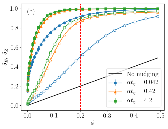
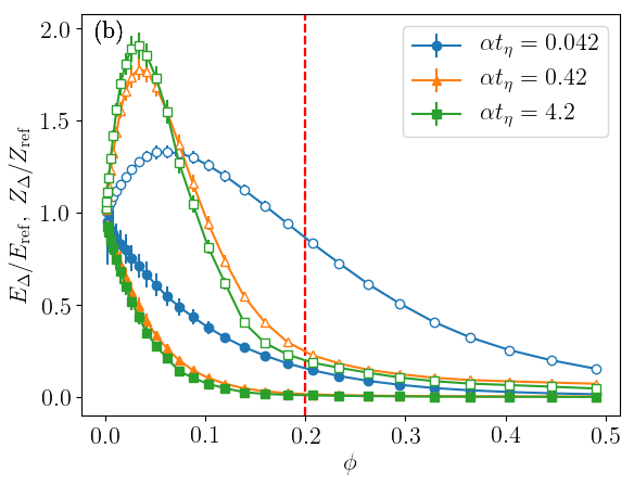
Figure 4: (a): Values of the velocity correlations $\delta_{E}$ (filled symbols) and the vorticity correlations $\delta_{Z}$ (empty symbols). (b) Values of the energy error $E_{\Delta}/E_{\rm ref}$ (filled symbols) and the enstrophy errors $Z_{\Delta}/Z_{\rm ref}$ (empty symbols). All values are plotted at changing volume fraction $\phi$ for different values of the nudging amplitude $\alpha$. Solid line in panel (a) represents the linear scaling expected for no effects of nudging (see text). The dashed red vertical lines mark the value $\phi_{c}=0.2$ as the typical estimate for transition to maximum synchronization in these sets-up. Here and in all figures error bars are always plotted, when they are not visible it means that they are smaller than the symbol size.

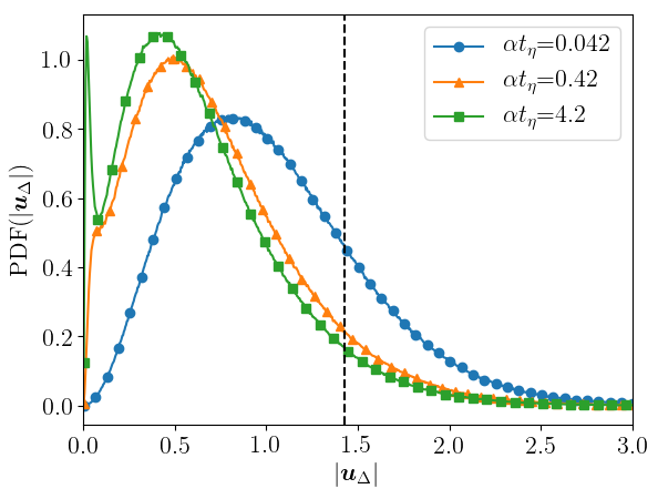
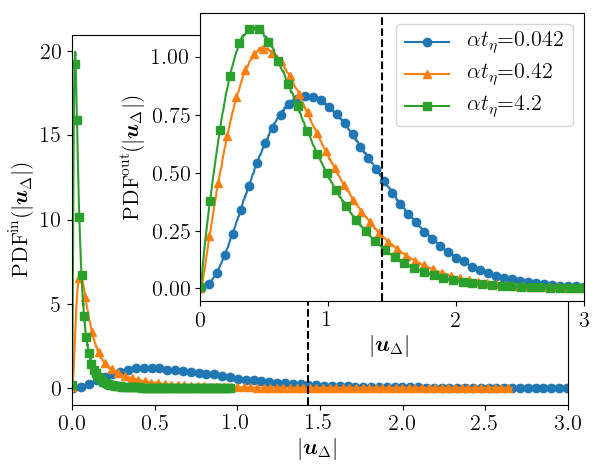
Figure 5: Histograms of the point-by-point reconstructing error $|\bm{u}_{\Delta}|$ measured in the whole volume (top), only inside the nudging regions (bottom) and only outside (inset). The vertical dashed line represent $\langle|{\bm{u}}_{\rm ref}|\rangle$.

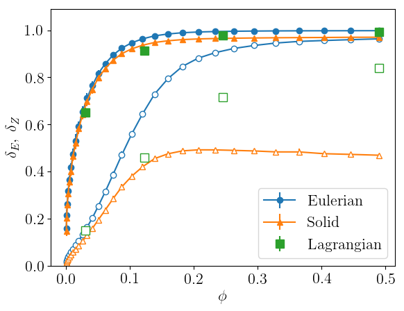
Figure 6: Values of the velocity correlations $\delta_{E}$ (filled symbols), and the vorticity correlations $\delta_{Z}$ (empty symbols) as a function of the volume fraction $\phi$ for different nudging protocols.

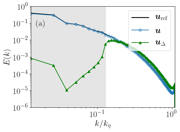
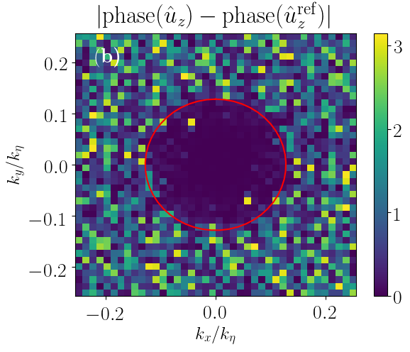
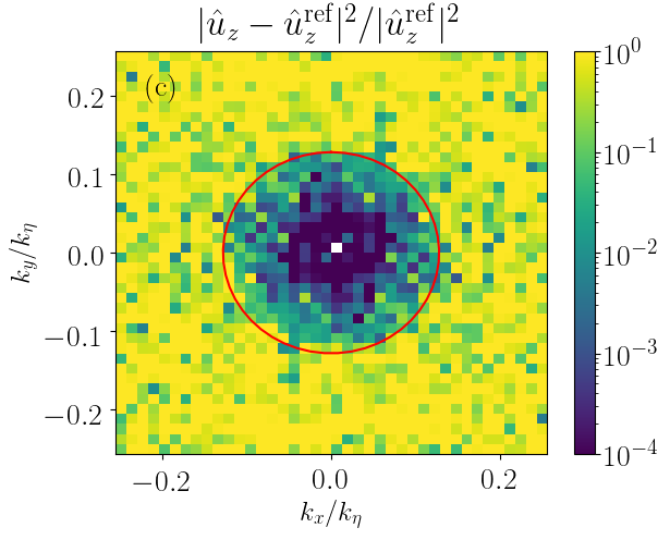
Figure 7: (a) Energy spectra for the nudged/reconstructed, ${\bm{u}}$, the reference, ${\bm{u}}_{\rm ref}$ and the error, ${\bm{u}}_{\Delta}$ fields. The grey area indicates the nudged scales, $k<k_{n}$. (b) Point-by-point error between the phases of the nudged/reconstructed field and the reference one in the $k_{z}=0$ Fourier plane. (c) The same of panel (b) but for the normalized amplitudes of the z component. The red circle defines $k_{n}$

II.2 Numerical protocols

Type	$E_{\rm ref}$	$\mathrm{Re}$	$\nu$	$t_{L}$	$t_{\eta}$	${k}_{\eta}$	$N^{3}$
RUN1	1.20	3900	0.0025	4.06	0.0042	78	$256^{3}$
RUN2	1.27	25000	0.0004	3.94	0.00062	317	$1024^{3}$

Table 1: Parameters used for the different reference simulations experiments. All the respective nudged simulations had the same parameters. The code uses a two step Adams Bashfort scheme for the time integration, and the “2/3 rule” for dealiasing. The values listed are the total kinetic energy $E=1/2\langle|{\bm{u}}_{\rm ref}|\rangle^{2}$, the Reynolds number $\mathrm{Re}=L(2E)^{1/2}/\nu$, the viscosity $\nu$, the eddy turnover time $t_{L}=L/(2E)^{1/2}$, the Kolmogorov timescale $t_{\eta}=\nu L/(2E)^{3/2}$, the Kolmogorov wavenumber $k_{\eta}=(\nu^{3}L/(2E)^{3/2})^{-1/4}$, and the number of grid points $N^{3}$. The largest scale of the flow $L$ is equal to $2\pi$ in all simulations. In both cases $\bm{f}_{\rm ref}$ is a randomly-generated, quenched in time, isotropic field with support on wavenumbers with amplitudes $k\in[1,2]$ whose Fourier coefficients are given by $\bm{\hat{f}}_{{\rm ref}}({{\bm{k}}})=f_{0}k^{-7/2}e^{i\theta_{\bm{k}}}$, where $\theta_{\bm{k}}$ are random in $[0,2\pi)$ and $f_{0}=0.02$.

In our study, the reference true data $\bm{u}_{\rm ref}$ is generated by numerically solving the Navier-Stokes equations (1), instead of using experimental measurements or field observations. The obvious advantage is that we can benchmark the reconstruction capabilities of nudging in a fully quantitative way, as we have access to the truth in every point in space and at every scale. Two different reference sets were produced, at medium and high Reynolds number (see Table 1 where all the details of the numerical methods used to solve (1) and (2) are given). In the rest of the paper, all values are made dimensionless by fixing the kinetic energy, the size of the box, and the viscosity. The exact protocol adopted is the following. Starting from rest, we evolve (1) until the system reaches a stationary state (marking this moment as $t=0$). Then we run for 10 turn over times (marking the final moment $t=T$), saving the fields at high frequency. We then solve (2) in the interval $t\in[0,T]$, using as initial condition $\mathcal{I}\bm{u}_{\rm ref}(\bm{x},t=0)$ and inputting the linearly interpolated field $\bm{u}^{\tau}_{\rm ref}$ into the nudging term. This is done for different values of $\alpha$ and $\tau$, and for the different filters $\mathcal{I}$ (Configuration Eulerian/Lagrangian or Fourier). The implementation of the point measurement based filter, (3), is a bit delicate. As we do not have any other injection mechanism in (2), nudging only in points (i.e. one grid point) makes it difficult to inject enough energy in order to maintain a stationary simulation with comparable $Re$. For this reason we actually nudge in small spheres of radius $r=1.25\eta$ centered around points $\bm{X}_{i}$. For the Eulerian set-up, these points were always placed on a uniform equispaced three dimensional grid covering the whole simulation box, so the only controlling parameter is the total number of probes $N_{p}$. The number we use to characterize each grid is the volume fraction:

$$\phi=N_{p}\frac{(4/3)\pi r^{3}}{L^{3}},$$ (6)

which is the ratio between the nudged and the total volumes. There are two useful wavenumbers that can be defined:

$$k_{l}=\frac{2\pi N^{1/3}_{p}}{L},\qquad k_{r}=\frac{2\pi}{r}.$$ (7)

where $k_{l}$ is associated with the minimum distance between probes and $k_{r}$ with the probe size. For the Lagrangian set-up, the protocol is similar with the only difference that the probe positions will move in time following the equation of a fluid tracer:

$$\bm{\dot{}}X_{i}(t)={\bm{u}}_{{\rm ref}}({\bm{X}}_{i}(t),t).$$ (8)

In Fig. 2 we give a first qualitative anticipation of both protocols, showing a 3D rendering of the reference field, of the probe distributions (nudging stations) and of the reconstructed flow for both Eulerian and Lagrangian nudging at high Reynolds. As a third variation, we will also explore nudging with spherical probes (placed on an Eulerian grid) where the velocity is fixed to have the same value of the one assumed in the center, making the filtered field $\mathcal{I}{\bm{u}}_{\rm ref}$ piece-wise constant and mimicking the results from a localized reference field measurement. We refer to this scheme as “solid” nudging.

II.3 Quantification of errors and correlations

We start by defining the difference between the two fields (error field) at every space-time point:

$$\bm{u}_{\Delta}(\bm{x},t)=\bm{u}(\bm{x},t)-{\bm{u}}_{\rm ref}(\bm{x},t).$$ (9)

Then, in order to quantify the nudging performances for turbulent DA at both large and small-scales we define the relative errors in the point-to-point energy and enstrophy reconstruction, based on the time-averaged $L_{2}$ norm:

$$\frac{E_{\Delta}}{E_{{\rm ref}}}=\frac{\langle|\bm{u}_{\Delta}|^{2}\rangle}{\langle|{\bm{u}}_{\rm ref}|^{2}\rangle},\qquad\frac{Z_{\Delta}}{Z_{\rm ref}}=\frac{\langle|{\bm{\omega}}_{\Delta}|^{2}\rangle}{\langle|{\bm{\omega}}_{\rm ref}|^{2}\rangle},$$ (10)

where ${\bm{\omega}}=\bm{\nabla}\times{\bm{u}}$ is the vorticity field and the average is defined as the mean on the whole volume, $V$, and on the whole experiment duration, $T$: $\langle\bullet\rangle=1/(T\,V)\int_{0}^{T}dt\int_{V}d{\bm{x}}\,(\bullet)$. We sometimes look at the temporal variations too, in those cases we explicitly remark that what we are showing depends on time. So, for example, the time evolution of the energy of a nudge simulation will be referred to as $E(t)$.

In order to have a scale-by-scale control of the degree of synchronization we introduce the energy spectrum of the difference between the nudged and the reference field, given by

$$E_{\Delta}(k,t)=\frac{1}{2}\sum_{k\leq|{\bm{k}}|<k+1}|\hat{\bm{u}}_{\Delta}({\bm{k}},t)|^{2}.$$ (11)

The two most informative measures of the success of reconstruction at large/small scales are based on velocity/vorticity field correlations

$$\delta_{E}=\frac{\langle\bm{u}\cdot\bm{u}_{\rm ref}\rangle}{\langle|{\bm{u}}|\rangle\langle|{\bm{u}}_{\rm ref}|\rangle},\qquad\delta_{Z}=\frac{\langle\bm{\omega}\cdot\bm{\omega}_{\rm ref}\rangle}{\langle|{\bm{\omega}}|\rangle\langle|{\bm{\omega}}_{\rm ref}|\rangle}.$$ (12)

Both quantities, will give a good account of how much the nudged fields is close to the reference one independently of the absolute values of each field (see later). Evidently, we have:

$$-1\leq\delta_{E},\delta_{Z}\leq 1.$$ (13)

Finally, it will be instructive to look also at the probability distribution function (PDF) of the point-wise error, $|{\bm{u}}_{\Delta}({\bm{x}},t)|$ in order to understand specific issues connected to worst-case scenarios and/or whether there are spatial and/or topological structures that are better reconstructed. The latter point might not be so relevant for isotropic turbulence but it is a key issue in non-isotropic conditions, like in the presence of boundaries or large scale shear, as often happens in nature or in applied turbulent realizations.

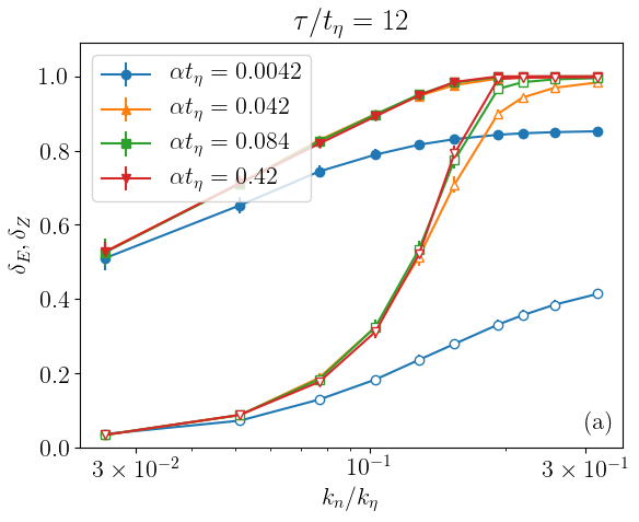
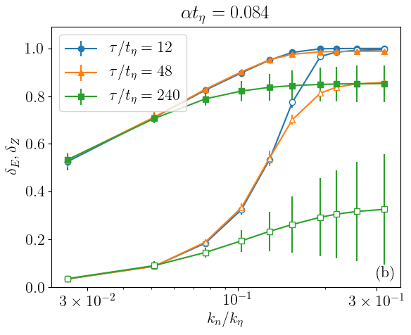
Figure 8: Values of the velocity correlations $\delta_{E}$ (filled symbols), and the vorticity correlations $\delta_{Z}$ (empty symbols) as a function of the maximum nudged wavenumber, $k_{n}$, for different values of the nudging amplitude, $\alpha$, and the interpolation time, $\tau$. In (a) $\tau/t_{\eta}=12$, in (b) $\alpha t_{\eta}=0.084$.

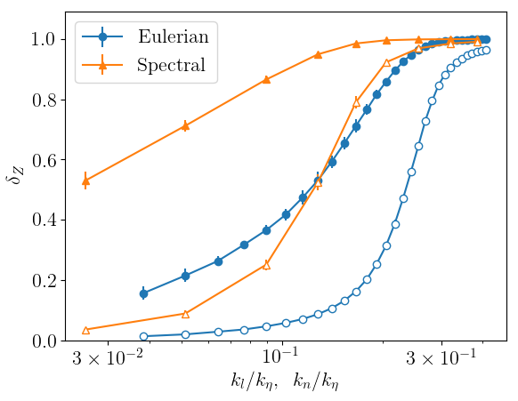
Figure 9: Values of the velocity correlations, $\delta_{E}$ (filled symbols), and the vorticity correlations, $\delta_{Z}$ (empty symbols), as a function of the maximum nudged wavenumber, $k_{n}$ (spectral case), or the mean nudged wavelength, $k_{l}$ (Eulerian case).

III Results

III.1 Nudging in configuration space

We start by studying the case of nudging in configuration space, where the penalty term acts in confined regions in space. From Fig. 2 we qualitatively see that the nudged flows (right panels) develop large-scale structures very close to the reference fields (left), even though nudging only acts locally. In this section we will focus on the effects of varying the nudging amplitude $\alpha$ and the nudged volume fraction $\phi$. In all simulations, the temporal interpolation $\tau/t_{\eta}=25$ and only data from RUN1 were used (see Table 1). We will study the response at varying the time-interpolation cadence, $\tau$, in Sec. III.2.

In Fig. 3a we show the evolution of the total energy for two nudged simulations, with $\phi=0.05$ and $\phi=0.23$. Both have $\alpha t_{\eta}=0.42$. The evolution of the total reference energy is also shown. As explained above, the initial condition of the nudged simulations is given by filtered reference at $t=0$, so they would look just like the middle panel in Fig. 2. It takes about one eddy turn over time for the nudged simulations to reach the stationary state, and to synchronize with the reference evolution, as seen in Fig. 3a. The evolution of the energy shows some very interesting features. First, the energy of the nudged field is always smaller than that of the reference field. Second, nudging a higher volume fraction does indeed inject more energy and make the nudged system resemble the reference one more closely. It is important to remember that aside from the nudging term, no energy is being injected in the simulations as there is no external forcing mechanism present in (2). Third –and probably most striking–, the nudged simulations is always able to follow the dynamical fluctuations of the reference field even in the presence of an appreciable amplitude mismatch. The latter, is the indication that we can have good statistical correlations among the two fields without complete synchronization. This will be put in more quantitative terms below.

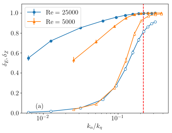
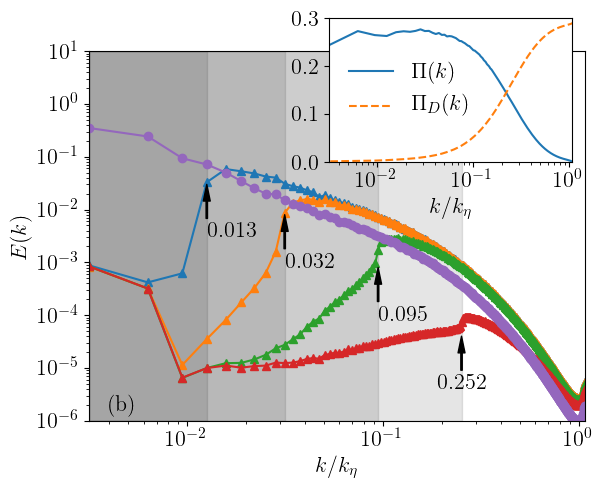
Figure 10: (a) Values of the velocity correlations $\delta_{E}$ (filled symbols), and the vorticity correlations $\delta_{Z}$ (empty symbols) as a function of the maximum nudged wavenumber $k_{n}$ for different values of the nudging amplitude $\alpha$ and the interpolation time $\tau$. Red dashed line marks the $k_{c}\sim 0.2k_{\eta}$ value where transition-to-synchronization is obtained (b) Energy spectra of the reference simulation RUN2 (round markers) and spectra of the difference field $u_{\Delta}$ at different $k_{n}$ (triangular markers). The value of $k_{n}/k_{\eta}$ for each nudged simulation is annotated with arrows. Inset: non-linear and viscous contributions to the energy fluxes for the reference simulation RUN2.

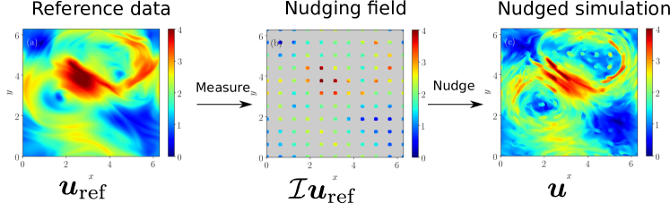
Figure 11: Visualizations of the local energy field of (a) a reference simulation ${\bm{u}}_{\rm ref}$, (b) a filtered field $\mathcal{I}{\bm{u}}_{\rm ref}$, (c) and a nudged simulation ${\bm{u}}$ of a rotating turbulent flow for $\phi=0.15$, $\alpha t_{\eta}=0.3$, and $\tau/t_{\eta}=33$. The reference simulation has $E_{\rm ref}=1.3$, $\nu=0.002$, $N^{3}=256^{3}$, $L=2\pi$, $t_{L}=3.89$, $t_{\eta}=0.003$, $\mathrm{Re}=5000$, and $\mathrm{Ro}=0.06$. The forcing, $\bm{f}_{\rm ref}$, is a randomly-generated, quenched in time, isotropic field with support on wavenumbers with amplitudes $k\in[1,2]$ whose Fourier coefficients are given by $\bm{\hat{f}}_{{\rm ref}}({{\bm{k}}})=f_{0}k^{-7/2}e^{i\theta_{\bm{k}}}$, where $\theta_{\bm{k}}$ are random in $[0,2\pi)$ and $f_{0}=0.005$.

In Figs. 3b and 3c we compare the instantaneous energy spectra of (i) the total reference field, ${\bm{u}}_{\mathrm{ref}}$; (ii) the filtered reference field used for nudging, $\mathcal{I}{\bm{u}}_{\mathrm{ref}}$; (iii) the resulting nudged field, ${\bm{u}}$ and the one which quantify the synchronization error (11) for two different nudging volume fractions $\phi=0.05$ and $\phi=0.23$, respectively. First, let us notice that the spectrum of $\mathcal{I}{\bm{u}}_{\mathrm{ref}}$ is mainly concentrated at small scales (large wavenumbers), with peaks in correspondence of the minimum distance between probes, $k_{l}$, and of the probe size, $k_{r}$, indicating that we are not supplying a large amount of information concerning the global large-scale motion (small wavenumbers). Despite of this, the scale-by-scale synchronization error, $E_{\Delta}(k,t)$, is smaller at large scales (small wavenumbers) than at small scales (large wavenumbers). Furthermore, in the case with $\phi=0.23$ (panel c) the errors remain small across all scales, indicating a very good global reconstruction and a transition to full synchronization already for such relatively small volume fraction.

In Fig. 4 we show, for 3 different values of $\alpha$, the correlations $\delta_{E}$ and $\delta_{Z}$, given by (12) and the normalized errors $E_{\Delta}/E_{\rm ref},Z_{\Delta}/Z_{\rm ref}$ given by (10) as a function of $\phi$. Good correlations and small relative errors in both the velocity and vorticity fields can be achieved with small nudged volume fractions. As one can see from the panel (a), already at $\phi\sim 0.2$ and for a nudging coefficient strong enough ($\alpha t_{\eta}\sim 0.5$) we can reconstruct both total energy and total enstrophy with an accuracy close to $90\%$. As expected, $\delta_{E}$ converges faster than $\delta_{Z}$, as it is determined by the large scales. For very small volume fractions, $\phi\ll 0.1$, the error is large, $E_{\Delta}/E_{\rm ref}=Z_{\Delta}/Z_{\rm ref}=1$, as the nudging field is almost equal to zero due to the fact that very little energy is injected into the system. As more energy is injected, $\phi\sim 0.05$ the relative error in the enstrophy increase at the beginning while the one in the energy always decreases. This is because the velocity field can generate correlations more easily, while the vorticity field does not, so for $\phi\ll 0.1$ one gets:

$$\frac{Z_{\Delta}}{Z_{\rm ref}} =\frac{\langle|{\bm{\omega}}-{\bm{\omega}}_{\rm ref}|^{2}\rangle}{\langle|{\bm{\omega}}_{\rm ref}|^{2}\rangle}\approx\frac{\langle|{\bm{\omega}}|^{2}\rangle+|\langle{\bm{\omega}}_{\rm ref}|^{2}\rangle}{\langle|{\bm{\omega}}_{\rm ref}|^{2}\rangle}\approx 2,$$

where we have used that $\langle{\bm{\omega}}\cdot{\bm{\omega}}_{\rm ref}\rangle\approx 0$ and that $\langle|{\bm{\omega}}|^{2}\rangle\approx\langle|{\bm{\omega}}_{\rm ref}|^{2}\rangle$. By comparing the behaviour for the three different values of $t_{\eta}\alpha$ one sees that by increasing $\alpha$ the transition to synchronization becomes sharper and little improvement is obtained as soon as $\alpha$ is of the same order of the highest frequency in the turbulent flow, $\sim 1/t_{\eta}$. The key parameter that drives the transition to synchronization is the volume fraction, and we can estimate the saturation to maximum achievable reconstruction for

$$\phi_{c}\sim 0.2$$

. In Fig. 4 we also plot the naive expectation obtained by supposing that nudging works only where we supply the information and gives fully uncorrelated results otherwise. In this case, the correlation coefficients would just scale as the volume fraction, $\phi$ (solid line in Fig. 4a).

In Fig. 5 we show the PDF for the point-by-point error, $|{\bm{u}}_{\Delta}|=|{\bm{u}}-{\bm{u}}_{\rm ref}|$, with the statistics taken over the whole volume (top panel), only inside the nudged regions (bottom panel), and only outside the nudged regions (inset), for different values of $\alpha t_{\eta}$ and with $\phi=0.05$. In accordance with Fig. 2, the errors inside the nudged regions are usually quite small, especially if compared with the mean $\langle|{\bm{u}}_{\rm ref}|\rangle$, denoted by the dashed vertical line in each figure. The statistics outside the nudged regions dominate the statistics over the whole volume, as the volume fraction is small. Increasing $\alpha$ pushes the mean and the mode of the errors closer to zero, without producing any fat tails in the distribution.

Finally, in Fig. 6 we compare the three different ways of performing nudging in configuration space described in Sec. II.1, Eulerian nudging, Solid nudging, and Lagrangian nudging, by looking $\delta_{E}$ and $\delta_{Z}$ as function of the nudging volume fraction. In all three cases $\alpha t_{\eta}=0.40$ and $\tau/t_{\eta}=25$. As one can see from $\delta_{E}$, the velocity field gets well reconstructed by all schemes. On the other hand, $\delta_{Z}$ indicates that vorticity reconstruction does not work well for the ”solid” schemes, as one could have expected because of the lack of small-scales information for this case. Surprisingly, also Lagrangian nudging performs slightly worse. One possible explanation is that the movement of the probes does not leave enough time for the flow synchronization at each point. One possible way to fix this problem could be to implement delayed-coordinates nudging, where the past history of the data is also used at each instant to guide the reconstruction, as was proposed for much simpler dynamical systems in Pazó et al. (2016) and never applied to turbulence up to now.

III.2 Nudging in Fourier space

We now turn to characterize how nudging in Fourier space works. We analyze the effects of varying the nudging amplitude $\alpha$, the interpolation time $\tau$ and the maximum nudged wavenumber $k_{n}$ in (5). To get a first glimpse of spectral nudging, we show in Fig. 7a the instantaneous energy spectrum for the full reference field, ${\bm{u}}_{\rm ref}$, that of the corresponding nudged/reconstructed field, ${\bm{u}}$, and the scale-by-scale synchronization error, $E_{\Delta}(k,t)$, for a simulation with $\alpha t_{\eta}=0.042$, $\tau/t_{\eta}=25$, and $k_{n}/k_{\eta}=0.13$. The grey region indicate the nudged window $k\in[0:k_{n}]$. Nudging is able to synchronize the nudged scales correctly as seen by the fact that $E_{\Delta}(k,t)$ is very small for $k<k_{n}$, and also in Figs. 7b and  7c, where the synchronization error for an instantaneous realization of Fourier phases and amplitudes are shown, respectively. The red circle in Figs. 7b and  7c denotes the maximum nudged wavenumber $k_{n}$. Concerning the transition to synchronization we study now what happens at changing $k_{n}$. Figure 8 shows the equivalent of Fig. 4 but for Fourier nudging, i.e. $\delta_{E}$ and $\delta_{Z}$, as a function of $k_{n}/k_{\eta}$ for different values of $\alpha$ while keeping $\tau$ fixed (panel a), and for different values of $\tau$ while keeping $\alpha$ fixed (panel b). Velocity field correlations start at high values, already for small $k_{n}$, as the smallest wavenumbers contain most of the energy, but vorticity field correlations require a larger amount of modes to be nudged in order to build up. At around

$$k_{n}=k_{c}\approx 0.2k_{\eta},$$

both $\delta_{E}$ and $\delta_{Z}$ show perfect synchronization being both equal to one.

By looking at Fig. 7a, one recognize that $k/k_{\eta}=0.2$ is around the end of the inertial range, indicating that one has to nudge everything but the viscous modes in order to reach the transition-to-synchronization limit. A similar result was found by Lalescu et al. (2013), where, at difference from here, synchronization was studied by imposing the nudged modes to be equal to the reference ones (something similar to $\alpha\to\infty$) and by supplying also the exact external forcing field. It is important to remark that the $\#_{dof}$ necessary to control for full synchronization, $k_{c}\sim 0.2k_{\eta}$ implies that the number of modes being nudged is still much smaller compared to the total number of dof, around $1\%$ actually, as the system is three dimensional. From Fig. 8 we also see that similar to the case of nudging in configuration space, increasing $\alpha$ has a positive effect. As expected, decreasing $\tau$ has a negative effect. The smaller the scales that we nudge, the more sensitive they become to the choice of $\tau$. This is because each Fourier mode has a characteristic correlation time, given the sweeping time $\tau_{s}(k)\sim 1/(\sqrt{2E}k)$ Chen and Kraichnan (1989); Clark di Leoni et al. (2014, 2015), that becomes shorter the higher the wavenumber. So if the correlation time of a particular mode becomes shorter than the interpolation time $\tau$, the interpolation starts to introduce unwanted errors. In Figure 9 we show the value of $\delta_{E}$ and $\delta_{Z}$ for Fourier nudging as a function of $k_{n}/k_{\eta}$ and for configurations space nudging as a function of $k_{l}/k_{\eta}$. The functional behaviour is very similar, indicating that both Fourier and configuration degrees of freedoms play a similar role in driving the chaotic evolution of isotropic turbulence. In other words, there are not preferred leading variables that drive the global and local flow configuration. The situation can be obviously very different, whenever the flow is driven by boundary effects as in channel turbulence, external fields, as for convection and MHD or influenced by the global set-up as for rotation (see Sec. III.3).

The effect of increasing the Reynolds number is studied in Fig. 10a, where we compare velocity and vorticity correlations for RUN1 and RUN2 (see Table 1) as a function of $k_{n}/k_{\eta}$. The fact that these two scans collapse on top of each other when plotting against $k_{n}/k_{\eta}$ shows that $k_{\eta}$ is the determining scale here. This can be understood better when looking at the energy spectra and flux. Figure 10b shows the energy spectra when nudging at different $k_{n}$ for the high Reynolds case. We see that when correlations are high, the spectra of the differences stays small for non-nudged wavenumbers. The inset of the figure shows the non-linear, $\Pi(k)$, and dissipative, $\Pi_{D}(k)$ contributions to the energy flux Alexakis and Biferale (2018) for the reference simulation (RUN2). The value of $k_{n}/k_{\eta}$ for which synchronization is achieved is the same value at which the dissipation flux and the energy flux become equivalent, but it is smaller than that at which dissipation completely dominates. This certifies that one has to nudge all the scales dominated by inertial effects in order to have a complete synchronization of the nudged flow with respect to the reference data. It is important to note that the Reynolds number of RUN2 is quite high, specially compared to the standard simulations done in other studies of Data Assimilation.

Figure 12: Values of the velocity correlations $\delta_{E}$, and the vorticity correlations $\delta_{Z}$ (empty symbols) as a function of the volume fraction $\phi$ for homogeneous and isotropic turbulence (HIT) or under rotation. The HIT simulations have $\alpha t_{\eta}=0.42$ and $\tau/t_{\eta}=25$, and the rotating turbulnce ones have $\alpha t_{\eta}=0.3$, and $\tau/t_{\eta}=33$.

III.3 Nudging under the presence of large scale structures

Finally, we show the results of nudging a system where large scale structures are present. As we mentioned in Sec. III.1, it is reasonable to expect that different systems can show different sensitivity to a given nudging scheme. Homogeneous and isotropic turbulence can be considered the worst case scenario as it lacks large scale coherent structures. In order to show that nudging can indeed be more efficient in the presence of some coherency into the system, we applied it to a rotating turbulent flow. Rotating turbulence is known for generating large columnar vortices with a strong translational symmetry in the direction parallel to the rotation axis Davidson (2013); Sen et al. (2012); Campagne et al. (2015); Biferale et al. (2016). It is known that nudging can reconstruct the inverse cascade present in rotating flows Clark Di Leoni et al. (2018), although this was shown only for spectral nudging. Equations (1) and (2) were modified by adding a Coriolis term of the form $-2\Omega\hat{{\bm{z}}}\times{\bm{u}}$, with $\Omega$ being the rotation frequency (see caption of Fig. 11 for more details on the simulations)). Figure 11 shows a visualization of horizontal slices of the energy of the full reference field, of the filtered/nudging field, and of the nudged/reconstructed field with applications of the protocol on the configuration domain. The aforementioned large scale structures are quite easy to spot, and it is evident how nudging works better in this scenario. Figure 12 compares the value of $\delta_{E}$ and $\delta_{Z}$ for one of the previous cases with nudging homogeneous isotropic turbulence and one case of nudging rotating turbulence. When the flow is under rotation, nudging is able to synchronize both the velocity and vorticity fields to the reference data at much lower volume fractions. This indicates that nudging can be a very powerful tool in problems that have large scale structures but are still nonlinear and chaotic.

IV Conclusions

We have presented the first systematic application of nudging to three dimensional homogeneous and isotropic turbulence for big-data assimilation (high Reynolds number regime). We have investigated the transition to full or scale-by-scale synchronization at changing the quantity and the quality (type) of information used. In particular, we have implemented nudging with measurements of (i) field values on a fixed number of spatial locations (Eulerian case), (ii) Fourier coefficients of the fields on a fixed range of wavenumbers (Fourier case), or (iii) field values along a set of moving probes inside the flow (Lagrangian case). Concerning the quantity of information we have shown that full synchronization is achieved as soon as the $\#_{dof}$ supplied by the nudging field covers a range of scales that is about one quarter of the dissipative Kolmogorov wavenumber (i.e. the largest wavenumber where non-linear inertial degrees-of-freedom are still active), coinciding with the scale at where inertial and viscous fluxes match each other. We have tested this at both moderate and high Reynolds numbers, where $k_{\eta}\sim k_{0}Re^{3/4}$, and $k_{0}$ is the energy containing scale. Similarly for nudging in configuration space, the critical volume fraction to reach synchronization is $\phi_{c}\sim 0.2$. We found that nudging in Fourier space improves data reconstruction, although paying the price that is more difficult to apply in realistic field-data applications. Concerning the quality of information we found that inputting Lagrangian data tends to deteriorate the ability to reconstruct but opens a much more flexible tools for environmental applications. It is also important to note that the fields be reconstruct have many points (in the order of $10^{7}$), so even at high volume fractions, applying a smooth three dimensional interpolation scheme in order to try to reconstruct the fields could be prohibtely expensive. Finally, we applied nudging to a turbulent rotating flow, we showed that despite the dynamics being richer with a split forward and backward energy cascade Alexakis and Biferale (2018); Davidson (2013); Pope (2000), the presence of large scale coherent structures helps nudging to reconstruct the reference flow at lower volume fractions than in the isotropic case, an important fact for many potential applications.

It is important to remark that our implementation of nudging is different from the usual one, because we do not supply information about the external forcing mechanisms in the nudge/reconstructed field evolution. This is done on purpose, to broaden its applicability to realistic conditions that are often encountered in the labs or in the open fields. Furthermore, the application of nudging to big-data goes well beyond the data-assimilation scope, as it can be seen as an unbiased equation-informed tool for classification of complex fields Clark Di Leoni et al. (2018) and/or as a tool to highlight hierarchy of correlations inside fluid turbulent applications, thanks to the mapping from input to output data mediated by the equations of motion. For example, it is tempting to imagine that nudging could be used in thermal Rayleigh-Bénard convection and in MHD to understand the casual correlation between temperature or magnetic fields with the velocity field and in bounded flows to disentangle the relative importance of near-wall regions wrt to bulk for driving the scale and location dependent turbulent fluctuations. Work in this direction will be reported elsewhere.