Influence of transverse field on the spin-3/2 Blume-Capel model on rectangular lattice

Abstract

Transverse field effect on thermodynamic properties of the spin-3/2 Blume-Capel model on rectangular lattice in which the interactions in perpendicular directions differ in signs is studied within the mean field approximation. Phase diagrams in the (transverse field, temperature) plane are constructed for various values of single-ion anisotropy.

1 Introduction

Modern statistical theory of condensed media pays great attention to studies of the Ising model extensions that include single-ion anisotropy and higher-order types of exchange interactions. The strong interest in these models arises partly on account of the rich phase transition (PT) behaviour they display [1, 2, 3, 4, 5, 6, 7, 8, 9, 10, 11, 12, 13] and partly due to the fact that they find applications to a wide class of real objects [14, 15]. Thus, the spin-3/2 Blume-Emery-Griffiths model was proposed to explain phase transition in DyVO₄ qualitatively [16] and was proved to be useful to describe tricritical properties in ternary fluid mixtures [17]. The spin-3/2 Blume-Capel (BC) model, which is the partial case of the spin-3/2 Blume-Emery-Griffiths model, can be applied to study KEr(MoO₄)₂ [18, 19].

The spin-3/2 Ising-type models has been investigated by different techniques: using the mean field approximation (MFA) [16, 20, 17, 8, 12, 13]; two-particle cluster approximation as well as the Bethe approximation (the exact results for Bethe lattices) [21, 10, 11]; the effective field theory [23, 22]; the renormalization-group method [24]; Monte-Carlo simulations [20, 9, 25]; the transfer-matrix finite-size-scaling calculations [9].

It should be separately mentioned the papers where the spin-3/2 Ising-type models in transverse field were investigated. In [26] the ground state of the spin-3/2 BC model with transverse field was studied within the framework of the MFA and effective-field theory. Transverse field and single-ion anisotropy dependencies of magnetization were calculated and the phase diagram in the (transverse field, single-ion anisotropy) plane were constructed within the both methods. Within the effective-field theory with correlations the spin-3/2 BC model [27] and the spin-3/2 Ising model in a random longitudinal field [28] were investigated in the presence of transverse field.

All the works know to us on the spin-3/2 Ising model consider lattices with either ferromagnetic bilinear interactions or antiferromagnetic bilinear interactions. In this work we will investigate within the MFA the transverse field influence on thermodynamical characteristics of the spin-3/2 Blume-Capel model

$$H=-\sum_{i=1}^{L}\sum_{j=1}^{L}\Big{[}\Gamma^{z}S_{i,j}^{z}+\Gamma^{x}S_{i,j}^{x}+D(S_{i,j}^{z})^{2}\Big{]}$$ (1)

$$-\sum_{i=1}^{L}\sum_{j=1}^{L}\Big{[}K^{\rm F}S_{i,j}^{z}S_{i+1,j}^{z}+K^{\rm AF}S_{i,j}^{z}S_{i,j+1}^{z}\Big{]}$$

on the rectangular lattice with the ferromagnetic bilinear short-range interaction ($K^{\rm F}>0$) in one direction and the antiferromagnetic one ($K^{\rm AF}<0$) in the perpendicular direction (as in KEr(MoO₄)₂). $\Gamma^{z}$ and $\Gamma^{x}$ are the longitudinal and transverse magnetic fields, $D$ is the single-ion anisotropy.

2 Mean field approximation

Within the mean field approximation [26, 29, 30, 31] Hamiltonian (1) can be expressed as

$$H=\sum_{i_{A}=1}^{N/2}H_{i_{A}}+\sum_{i_{B}=1}^{N/2}H_{i_{B}}+{\textstyle\frac{N}{2}}K^{\rm F}(m_{A}^{2}+m_{B}^{2})+NK^{\rm AF}m_{A}m_{B}.$$ (2)

Here $A$ and $B$ refer to two sublattices, $N=L^{2}$ is the total number of spins, $m_{A}=\langle S^{z}_{i_{A}}\rangle$ and $m_{B}=\langle S^{z}_{i_{B}}\rangle$ are magnetizations of the sublattices, $H_{i_{A}}$ and $H_{i_{B}}$ are the so-called one-particle Hamiltonians

$$H_{i_{\alpha}}=-\varkappa_{\alpha}S^{z}_{i_{\alpha}}-\Gamma^{x}S^{x}_{i_{\alpha}}-D(S^{z}_{i_{\alpha}})^{2},$$ (3)

$$\varkappa_{\alpha}=\Gamma^{z}+2K^{\rm F}m_{\alpha}+2K^{\rm AF}m_{\beta},\qquad(\alpha,\beta=A,B).$$ (4)

In order to obtain the free energy

$$F=-{\textstyle\frac{N}{2}}k_{B}T\;\!{\rm ln}Z_{1_{A}}-{\textstyle\frac{N}{2}}k_{B}T\;\!{\rm ln}Z_{1_{B}}+{\textstyle\frac{N}{2}}K^{\rm F}(m_{A}^{2}+m_{B}^{2})+NK^{\rm AF}m_{A}m_{B},$$ (5)

$$Z_{1_{\alpha}}={\rm Sp}\;\!{\rm e}^{-H_{1_{\alpha}}/(k_{\rm B}T)}$$ (6)

of model (1) within MFA we need to calculate first the one-particle partition functions $Z_{1_{\alpha}}$. One-particle Hamiltonian (3) is defined on a one-spin basis which consists of four eigenstates of the $S_{i}^{z}$ operator.

$$|1\rangle \left(\!\!\begin{array}[]{c}1\\ 0\\ 0\\ 0\end{array}\!\!\right) |2\rangle \left(\!\!\begin{array}[]{c}0\\ 1\\ 0\\ 0\end{array}\!\!\right) |3\rangle \left(\!\!\begin{array}[]{c}0\\ 0\\ 1\\ 0\end{array}\!\!\right) |4\rangle \left(\!\!\begin{array}[]{c}0\\ 0\\ 0\\ 1\end{array}\!\!\right)$$ 3/2 1/2 -1/2 -3/2
(25)

In this representation, the one-particle Hamiltonian reads

$$\langle i|H_{1_{\alpha}}|j\rangle=-\left(\!\begin{array}[]{cccc}-{\textstyle\frac{3}{2}}\varkappa_{\alpha}\!-\!{\textstyle\frac{9}{4}}D&{}-\!{\textstyle\frac{\sqrt{3}}{2}}\Gamma^{x}&{}0&{}0\vspace{0.25cm}\\ \!\!\!-{\textstyle\frac{\sqrt{3}}{2}}\Gamma^{x}&\!\!\!{}-\!{\textstyle\frac{1}{2}}\varkappa_{\alpha}\!-\!{\textstyle\frac{1}{4}}D&{}-\Gamma^{x}&{}0\vspace{0.25cm}\\ 0&\!\!\!\!\!\!{}-\Gamma^{x}&\!\!{}{\textstyle\frac{1}{2}}\varkappa_{\alpha}\!-\!{\textstyle\frac{1}{4}}D&{}-\!{\textstyle\frac{\sqrt{3}}{2}}\Gamma^{x}\vspace{0.25cm}\\ 0&{}\!\!0&\!\!\!{}-\!{\textstyle\frac{\sqrt{3}}{2}}\Gamma^{x}&\;{}{\textstyle\frac{3}{2}}\varkappa_{\alpha}\!-\!{\textstyle\frac{9}{4}}D\end{array}\!\right).$$ (30)

Based on (6) and (LABEL:f5) we obtain

$$Z_{1_{\alpha}}=\sum_{\nu=1}^{4}{\rm e}^{-(E_{\alpha})_{\nu}/(k_{\rm B}T)}\;,$$ (31)

where the eigenvalues $(E_{\alpha})_{\nu}$ of matrix (LABEL:f5) are roots of the following equation of the 4^th order

$$E_{\alpha}^{4}+5DE_{\alpha}^{3}+a_{\alpha}E_{\alpha}^{2}+b_{\alpha}E_{\alpha}+c_{\alpha}=0.$$ (32)

Here we use the notations:

$$a_{\alpha}={\textstyle\frac{59}{8}}D^{2}-{\textstyle\frac{5}{2}}\varkappa_{\alpha}^{2}-{\textstyle\frac{5}{2}}(\Gamma^{x})^{2},$$ (33)

$$b_{\alpha}=D[{\textstyle\frac{45}{16}}D^{2}-{\textstyle\frac{9}{4}}\varkappa_{\alpha}^{2}-{\textstyle\frac{33}{4}}(\Gamma^{x})^{2}],$$

$$c_{\alpha}={\textstyle\frac{81}{256}}D^{4}-{\textstyle\frac{45}{32}}D^{2}\varkappa_{\alpha}^{2}+{\textstyle\frac{9}{8}}(\Gamma^{x})^{2}\varkappa_{\alpha}^{2}-{\textstyle\frac{189}{32}}D^{2}(\Gamma^{x})^{2}+{\textstyle\frac{9}{16}}\varkappa_{\alpha}^{4}+{\textstyle\frac{9}{16}}(\Gamma^{x})^{4}.$$

It should be noted that the roots $(E_{\alpha})_{\nu}$ depend on both $m_{\alpha}$ and $m_{\beta}$ (see (4) and (33)).

Within the MFA the thermal expectation values $m_{\alpha}=\langle S^{z}_{i_{\alpha}}\rangle$ can be determined [19, 29, 30, 31, 32] from the conditions of extremum of the free energy with respect to them ($\partial F/\partial m_{A}=\partial F/\partial m_{B}=0$). These conditions yield the following system of equations for $m_{\alpha}$:

$$\frac{\varkappa_{A}}{Z_{1_{A}}}\sum_{\nu=1}^{4}{\rm e}^{-(E_{A})_{\nu}/(k_{\rm B}T)}(R_{A})_{\nu}+2m_{A}=0,$$ (34)

$$\frac{\varkappa_{B}}{Z_{1_{B}}}\sum_{\nu=1}^{4}{\rm e}^{-(E_{B})_{\nu}/(k_{\rm B}T)}(R_{B})_{\nu}+2m_{B}=0,$$

where

$$(R_{\alpha})_{\nu}=\frac{10(E_{\alpha})_{\nu}\!{}^{2}+9D(E_{\alpha})_{\nu}+{\textstyle\frac{45}{8}}D^{2}-{\textstyle\frac{9}{2}}(\Gamma^{x})^{2}-{\textstyle\frac{9}{2}}\varkappa_{\alpha}^{2}}{4(E_{\alpha})_{\nu}\!{}^{3}+15D(E_{\alpha})_{\nu}\!{}^{2}+2a_{\alpha}(E_{\alpha})_{\nu}+b_{\alpha}}\;.$$ (35)

3 Numerical analysis results

In this section we discuss the results of numerical calculation of model (1) for the case $\Gamma^{z}=0$ within the MFA.

Let us introduce the quantity $x$ which characterizes coupling between the interactions $K^{\rm AF}$ and $K^{\rm F}$:

$$K^{\rm F}=K(1+x),\qquad K^{\rm AF}=K(-1+x),\qquad x\in]-1,1[.$$ (36)

We emphasize that in a general case the solutions of the system of equations (34) corresponding to extrema of the free energy (5) depend on $x$. However, the solutions corresponding to the absolute minimum of the free energy (the sublattice magnetizations) do not depend on $x$ in the absence of the longitudinal magnetic field. This means that the MFA results for thermodynamic characteristics of model (1) with $\Gamma^{z}=0$ do not depend on $x$.

Let us explain this statement. It can be seen from the symmetry of Hamiltonian (1) at $\Gamma^{z}=0$ that there exists such a canonical transformation (inversion of all spins of one sublattice) which enable us to reduce the problem with $K^{\rm F}>0$ and $K^{\rm AF}<0$ to the one with two ferromagnetic interactions ${K}^{\rm F1}=K^{\rm F}$ and ${K}^{\rm F2}=-K^{\rm AF}$. This means that if the problem with the both ferromagnetic interactions is substituted by the one with the ferromagnetic and antiferromagnetic interactions the phase diagram does not change except the ferromagnetic phase is replaced by the antiferromagnetic one. Thus the antiferromagnetic ordering can only be realized in model (1) at $\Gamma^{z}=0$ (the antiferrimagnetic and ferrimagnetic orderings can exist only at $\Gamma^{z}\neq 0$).

On the other hand the MFA results (5) - (34) for model (1) at $m_{A}=-m_{B}$ (which takes place for solutions of system of equations (34) corresponding to absolute minima of free energy (5)) coincide with their counterparts (38) - (41) for the spin-3/2 BC model in transverse field on a rectangular lattice in which both interactions are antiferromagnetic (see appendix). This can be checked analytically. The MFA results for the latter model contain interactions $K_{1}$ and $K_{2}$ only in combination $K_{1}+K_{2}$. Thus the results for thermodynamic characteristics of model (1) at $\Gamma^{z}=0$ within the MFA depend on $K^{\rm AF}-K^{\rm F}$ (do not depend on $x$).

It should be noted that in cases (1) and (37) the lattices are divisible into sublattices in different manner.

In this section we shall use the following notation for the relative quantities (see also (36)):

$$t\!=k_{\rm B}T/K,\qquad d=D/K,\qquad h^{x}=\Gamma^{x}/K,$$

and the following three phases will be distinguished (see Refs. [8, 9, 11, 12, 13, 20, 22, 24, 25]):

$\bullet$ antiferromagnetic-3/2 phase (AF_3/2);

$\bullet$ antiferromagnetic-1/2 phase (AF_1/2);

$\bullet$ paramagnetic phase (P).

Here the identification of phases AF_3/2 and AF_1/2 has not a robust criterion as in the case of zero transverse field, because increase of $|h^{x}|$ leads to decrease of magnetizations of sublattices (at $t=0$ also). Thus at $h^{x}>0$ in the ground state the magnetizations $m_{A}$ and $m_{B}$ do not reach their “asymptotic” values $m_{A}=-m_{B}=3/2$ or $m_{A}=-m_{B}=1/2$ as it happens at $h^{x}=0$. In the ground state absolute values of magnetizations of sublattices correspond to the indices in the names of phases only at $h^{x}=0$.

It should be mentioned that such a classification of the ordered phases not only is far from perfection at $h^{x}\neq 0$, but also makes sense, basically, only in studies of the temperature dependencies of sublattice magnetizations. Moreover, sometimes we can not distinguish between phases AF_3/2 and AF_1/2. In this case we will denote this phase as AF.

We are able to distinguish these antiferromagnetic phases AF_3/2 and AF_1/2 in the following cases:

(i) in the ground state at $h^{x}=0$;

(ii) in the ground state at $h^{x}\neq 0$ in particular cases, provided that we have graphs of temperature dependencies of sublattice magnetizations in a sufficiently wide temperature interval and respective phase diagrams;

(iii) near the phase transition AF_3/2 $\leftrightarrow$ AF_1/2;

(iv) at $t>0$ outside of the phase transition AF_3/2 $\leftrightarrow$ AF_1/2 region in particular cases only (provided that we have graphs of temperature dependencies of magnetizations in a sufficiently wide temperature interval and respective phase diagrams).

Let us note that within the MFA for the $\Gamma^{z}=0$ case phase transitions between different antiferromagnetic phases can be only of the first order and transitions between antiferromagnetic and paramagnetic phases can be only of the second order.

It will be easier to understand the effects produced by the transverse field, if we at first briefly consider the results obtained for the case of zero transverse field [20, 33]. In Fig. 1 we present the phase diagram in the $(d,t)$ plane obtained within the MFA. The diagram contains a critical point (CP) inside the AF phase at $d=d_{\rm CP}\approx-1.95$ and a ground state phase boundary point (0P) inside the AF phase at $d=d_{\rm 0P}=-2.0$. For $d<d_{\rm 0P}$ the system undergoes the phase transition AF_1/2 $\rightarrow\;$P on increasing temperature. For $d\in[d_{\rm 0P},d_{\rm CP}]$ two PTs AF_3/2 $\rightarrow\;$AF_1/2 and AF $\rightarrow\;$P take place. For $d>d_{\rm CP}$ the temperature PT AF $\rightarrow\;$P is expected by the MFA (at $d\gg d_{\rm CP}$ we can only determine this transition as AF_3/2 $\rightarrow\;$P).

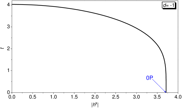
Figure 2: The $h^{x}$ vs $t$ phase diagram at $d=-1$. Thick solid line indicates the PT antiferromagnetic $\rightarrow\;$paramagnetic phase of the second order. The special point is the phase boundary point in the ground state (0P).

For $d\gg d_{\rm CP}$ (see Fig. 1) the topology of the $(h^{x},t)$ phase diagrams is the same as the topology of the diagram given in Fig. 2. At $|h^{x}|<h^{x}_{0P}$ ($h^{x}=h^{x}_{0P}$ is the coordinate of the ground state phase boundary point) the system undergoes the PT AF_3/2 $\rightarrow\;$P on increasing temperature. At $|h^{x}|>h^{x}_{0P}$ no temperature PT is expected by MFA.

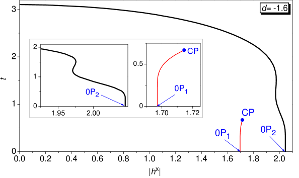
Figure 4: The $h^{x}$ vs $t$ phase diagram at $d=-1.6$. Thick solid line indicates the PT antiferromagnetic $\rightarrow\;$paramagnetic phase of the second order. Thin solid line indicates the first order PT between different antiferromagnetic phases. The special points are the critical point (CP) and the phase boundary points in the ground state (0P₁, 0P₂).

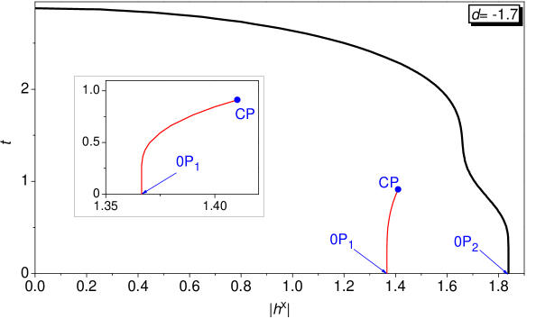
Figure 5: The same as in Fig. 4, but $d=-1.7$.

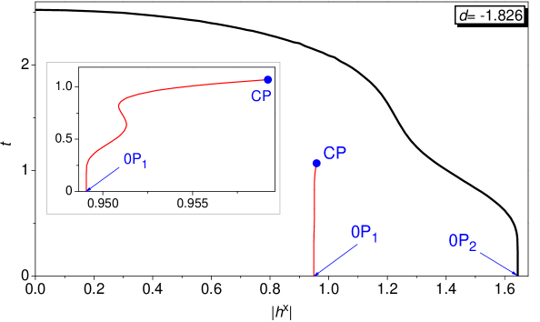
Figure 6: The same as in Fig. 4, but $d=-1.826$.

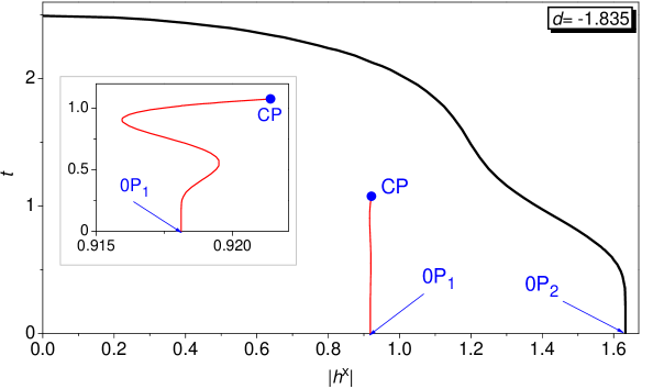
Figure 7: The same as in Fig. 4, but $d=-1.835$.

If single-ion anisotropy is close to $d_{\rm CP}$ and $d_{\rm 0P}$ (see Fig. 1) the topology of $(h^{x},t)$ phase diagrams can be of nine different types. Figs. 3 – 11 illustrate the major aspect of the changes in the topologies of $(h^{x},t)$ phase diagrams as we change $d$.

The phase diagram presented in Fig. 3 has a double re-entrant topology. A cascade of temperature phase transitions AF_3/2 $\rightarrow\;$P $\rightarrow\;$AF_3/2 $\rightarrow\;$P is possible at $h^{x}\in[2.269,2.281]$. For $h^{x}<2.269$ and $h^{x}\in]2.281,h^{x}_{0P}]$ the MFA yields single PT AF_3/2 $\rightarrow\;$P. For $h^{x}>h^{x}_{0P}$ no temperature PT is expected.

The $(h^{x},t)$ phase diagram for $d=-1.6$ (Fig. 4) has a double re-entrant topology and the CP inside the AF phase. The system undergoes the temperature PT AF_3/2 $\rightarrow\;$P at $|h^{x}|<h^{x}_{0P_{1}}$, two PTs AF_1/2 $\rightarrow\;$AF_3/2 and AF $\rightarrow\;$P at $|h^{x}|\in[h^{x}_{0P_{1}},h^{x}_{CP}]$ ($h^{x}=h^{x}_{CP}$ is a coordinate of the critical point), one PT AF $\rightarrow\;$P at $|h^{x}|\in]h^{x}_{CP},1.971]$, a cascade of transitions AF $\rightarrow\;$P $\rightarrow\;$AF $\rightarrow\;$P at $|h^{x}|\in]1.971,1.975]$ and one PT AF_1/2 $\rightarrow\;$P at $|h^{x}|\in]1.975,h^{x}_{0P_{2}}]$. At $|h^{x}|>h^{x}_{0P_{2}}$ PT is absent. It should be noted that in this case the AF $\rightarrow\;$P phase transition can be identified as AF_3/2 $\rightarrow\;$P or AF_1/2 $\rightarrow\;$P only at those values of $|h^{x}|$, which are much lower or much higher than $h^{x}_{CP}$, respectively.

At $d=-1.7$ the $(h^{x},t)$ phase diagram contains the CP inside the AF phase (see Fig. 5). The MFA yields the temperature PT AF $\rightarrow\;$P at $|h^{x}|<h^{x}_{0P_{1}}$, two transitions AF_1/2 $\rightarrow\;$AF_3/2 and AF $\rightarrow\;$P at $|h^{x}|\in[h^{x}_{0P_{1}},h^{x}_{CP}$], one PT AF $\rightarrow\;$P at $|h^{x}|\in]h^{x}_{CP},h^{x}_{0P_{2}}]$ and no PT at $|h^{x}|>h^{x}_{0P_{2}}$. In this case (as in the case $d=-1.6$) only at $|h^{x}|\ll h^{x}_{CP}$ and at $|h^{x}|\gg h^{x}_{CP}$ we can determine AF $\rightarrow\;$P phase transitions as AF_3/2 $\rightarrow\;$P and AF_1/2 $\rightarrow\;$P, respectively.

At $d=-1.826$ and $d=-1.835$ the $(h^{x},t)$ phase diagrams have a double re-entrant topology with the CP inside the AF phase (see Figs. 6, 7). But the changes of sublattice magnetizations temperature dependencies with changing $h^{x}$ are different for these both cases. For $d=-1.826$ and $d=-1.835$ at $|h^{x}|<h^{x}_{0P_{1}}$ and $|h^{x}|<0.916$, respectively, the system undergoes the temperature PT AF $\rightarrow\;$P. It should be noted that at sufficiently small values of $|h^{x}|$ we can determine it as AF_3/2 $\rightarrow\;$P. At $|h^{x}|\in[h^{x}_{0P_{1}},0.951]$ for the case $d=-1.826$ the system undergoes two phase transitions AF_1/2 $\rightarrow\;$AF_3/2 and AF $\rightarrow\;$P. At $|h^{x}|\in[0.916,h^{x}_{0P_{1}}]$ for the case $d=-1.835$ the system exhibits re-entrant behaviour AF_3/2 $\rightarrow\;$AF_1/2 $\rightarrow\;$AF_3/2 at low temperatures and undergoes the PT AF $\rightarrow\;$P at hight temperatures. For the both cases $d=-1.826$ and $d=-1.835$ at $|h^{x}|\in]0.951,0.9513]$ and at $|h^{x}|\in]h^{x}_{0P_{1}},0.9195$], respectively, the system exhibits in low temperature region double re-entrant behaviour AF_1/2 $\rightarrow\;$AF_3/2 $\rightarrow\;$AF_1/2 $\rightarrow\;$AF_3/2 and has the AF $\rightarrow\;$P phase transition in high temperature region. At $|h^{x}|\in]0.9513,h^{x}_{CP}]$ for the case $d=-1.826$ as well as at $|h^{x}|\in]0.9195,h^{x}_{CP}]$ for the case $d=-1.835$ the system undergoes two PTs AF_1/2 $\rightarrow\;$AF_3/2 and AF $\rightarrow\;$P. At $|h^{x}|\in]h^{x}_{CP},h^{x}_{0P_{2}}]$ for the cases $d=-1.826$ and $d=-1.835$ the PT AF $\rightarrow\;$P takes place. At sufficiently large values of $|h^{x}|$ we can determine this PT as AF_1/2 $\rightarrow\;$P. For the both cases at $|h^{x}|>h^{x}_{0P_{2}}$ the system is in the paramagnetic phase at any temperature.

The $(h^{x},t)$ phase diagram for $d=-1.845$ (Fig. 8) has topology with two re-entrant regions and the CP inside the AF phase. In this case the MFA yields the temperature PT AF $\rightarrow\;$P at $|h^{x}|<0.875$, a cascade of PTs AF_3/2 $\rightarrow\;$AF_1/2 $\rightarrow\;$AF_3/2 and AF $\rightarrow\;$P at $|h^{x}|\in[0.875,h^{x}_{CP}]$, two transitions AF_3/2 $\rightarrow\;$AF_1/2 and AF $\rightarrow\;$P at $|h^{x}|\in]h^{x}_{CP},h^{x}_{0P_{1}}]$, a cascade of PTs AF_1/2 $\rightarrow\;$AF_3/2 $\rightarrow\;$AF_1/2 and AF $\rightarrow\;$P at $|h^{x}|\in]h^{x}_{0P_{1}},0.884$], one PT AF $\rightarrow\;$P at $|h^{x}|\in]0.884,h^{x}_{0P_{2}}]$ and no PT at $|h^{x}|>h^{x}_{0P_{2}}$. In this case (as in those described below) we can only at sufficiently small values of $|h^{x}|$ ($|h^{x}|\ll h^{x}_{CP}$) and at sufficiently large values of $|h^{x}|$ ($|h^{x}|\gg h^{x}_{CP}$) determine AF $\rightarrow\;$P phase transitions as AF_3/2 $\rightarrow\;$P and AF_1/2 $\rightarrow\;$P transitions, respectively.

The phase diagram presented in Fig. 9 ($d=-1.9$) has topology with re-entrant region and the CP inside the AF phase. The system undergoes the temperature PT AF $\rightarrow\;$P at $|h^{x}|<h^{x}_{CP}$, two PTs AF_3/2 $\rightarrow\;$AF_1/2 and AF $\rightarrow\;$P at $|h^{x}|\in[h^{x}_{CP},h^{x}_{0P_{1}}]$, a cascade of three transitions AF_1/2 $\rightarrow\;$AF_3/2 $\rightarrow\;$AF_1/2 and AF $\rightarrow\;$P at $|h^{x}|\in]h^{x}_{0P_{1}},0.68136$], one PT AF $\rightarrow\;$P at $|h^{x}|\in]0.68136,h^{x}_{0P_{2}}]$ and no PT at $|h^{x}|>h^{x}_{0P_{2}}$.

In the case $d=-1.945$ (see Fig. 10) the $(h^{x},t)$ phase diagram has topology with the CP inside the AF phase and in the case $d=-1.96$ (Fig. 11) it has topology without a CP. In the case $d=-1.945$ at $|h^{x}|<h^{x}_{CP}$ the system undergoes the PT AF $\rightarrow\;$P. In the cases $d=-1.945$ and $d=-1.96$ at $|h^{x}|\in[h^{x}_{CP},h^{x}_{0P_{1}}]$ and $|h^{x}|\leq h^{x}_{0P_{1}}$, respectively, the system undergoes two transitions AF_3/2 $\rightarrow\;$AF_1/2 and AF $\rightarrow\;$P. At $|h^{x}|\in]h^{x}_{0P_{1}},h^{x}_{0P_{2}}]$ for $d=-1.945$ and $d=-1.96$ one PT AF $\rightarrow\;$P takes place. At $|h^{x}|>h^{x}_{0P_{2}}$ for the both cases the temperature transitions are absent.

For $d\ll d_{\rm CP}$ (see Fig. 1) the topology of the $(h^{x},t)$ phase diagrams within the MFA is the same as that of the diagram given in Fig. 12. At $|h^{x}|<h^{x}_{0P}$ the system undergoes the temperature PT AF_1/2 $\rightarrow\;$P. At $|h^{x}|>h^{x}_{0P}$ no temperature PT is expected by MFA.

Finally, let us briefly consider re-entrant phenomena. In our opinion the re-entrant and double re-entrant transitions both between ordered and disordered phases of the second order and between different ordered phases of the first order are caused by the competitions of the bilinear interactions (which in the considered model are described only by one parameter $K$) with the transverse field and the negative single-ion anisotropy. A similar re-entrances have been found, for example, in Refs. [2, 3, 4, 8, 12, 13, 28, 34] (see also [35]) within various techniques for different Ising models with spin $S>1/2$.

During the detailed investigation we have found that re-entrant and double re-entrant temperature PTs considered in this work occur in narrow regions (ranges) of parameters $h^{x}$ and $d$ (for the double re-entrant transitions between ordered and disordered phases of the second order see Fig. 13). They appear due to the cooperative effect: competition between $K$ and $\Gamma^{x}$ as well as competition between $K$ and negative $D$. There is no dominative contribution and none of the mentioned competitions leads to the re-entrant behaviour in its own right.

It should be noted that re-entrant topologies are equally well defined on the phase diagrams both in ($h^{x},t$) and in ($d,t$) planes (for the case of double re-entrant temperature PTs between ordered and disordered phases of the second order see the insert in Fig. 13).

Only a part of the phase diagram projection on the ($h^{x},d$) plane is presented in Fig. 13, where a region with cascades of double re-entrant phase transitions between ordered and disordered phases of the second order is marked. The regions, where re-entrant and double re-entrant temperature PTs between different ordered phases of the first order occur, have a qualitative appearance similar to the one shown in Fig. 13.

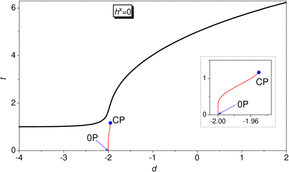
Figure 1: The $d$ vs $t$ phase diagram at $h^{x}=0$. Thick solid line indicates the PT antiferromagnetic $\rightarrow\;$paramagnetic phase of the second order. Thin solid line indicates the first order PT between different antiferromagnetic phases. The special points are the critical point (CP) and the phase boundary point in the ground state (0P).

Figure 3: The same as in Fig. 2, but $d=-1.5$.

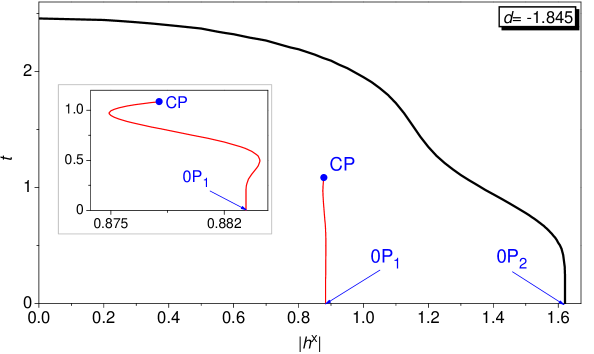
Figure 8: The same as in Fig. 4, but $d=-1.845$.

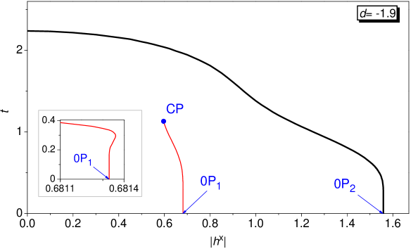
Figure 9: The same as in Fig. 4, but $d=-1.9$.

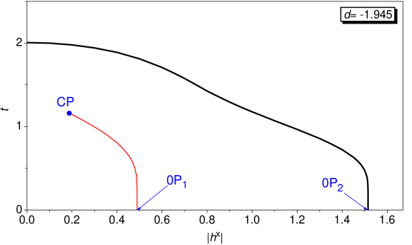
Figure 10: The same as in Fig. 4, but $d=-1.945$.

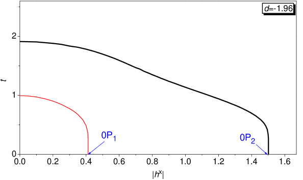
Figure 11: The same as in Fig. 4, but $d=-1.96$.

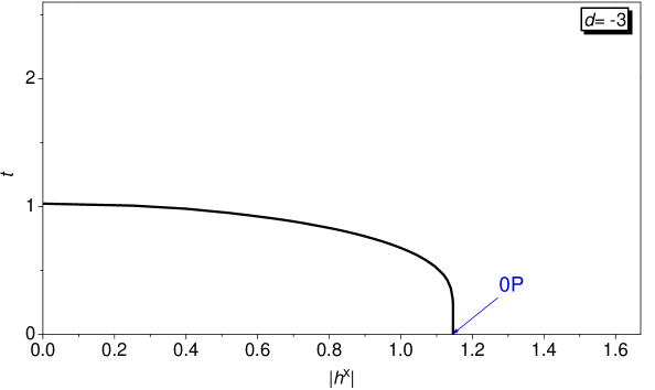
Figure 12: The same as in Fig. 2, but $d=-3$.

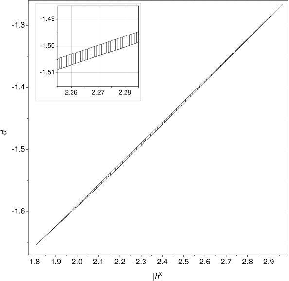
Figure 13: A part of the phase diagram projection on the $(h^{x},d)$ plane with a marked region (shaded area), where double re-entrant temperature phase transitions of the second order between ordered and disordered phases occur (see also Fig. 3).

4 Conclusions

The spin-3/2 Blume-Capel model with the transverse field on the rectangular lattice in which the interactions in perpendicular directions are of different signs has been studied within the mean field approximation. The transverse field vs temperature phase diagrams at different values of single-ion anisotropy are obtained in the absence of the longitudinal field. The phase diagrams presented in this paper illustrate the major aspects of the changes in topologies of the phase diagrams in the (transverse field, temperature) plane with changing the single-ion anisotropy.

It is established that in the case of zero longitudinal field the results for thermodynamic characteristics depend on the sum of absolute values of the interactions $|K^{\rm AF}|+K^{\rm F}$ and are independent on their ratio $K^{\rm AF}/K^{\rm F}$ if $|K^{\rm AF}|+K^{\rm F}$ is constant. Moreover, we ascertain also that the sublattice magnetization results of the investigated model coincide at $\Gamma^{z}=0$ with those of the spin-3/2 Blume-Capel model in transverse field on the rectangular lattice with both antiferromagnetic interactions (except that in these models the lattices are divisible into sublattices in different manner).

It is shown that at certain values of model parameters the double re-entrant temperature phase transitions AF_3/2 $\rightarrow\;$P $\rightarrow\;$AF_3/2 $\rightarrow\;$P and AF_1/2 $\rightarrow\;$AF_3/2 $\rightarrow\;$AF_1/2 $\rightarrow\;$AF_3/2 are possible.

Appendix A

Let us present the MFA result for the spin-3/2 Blume-Capel model

$$H=-\sum_{i=1}^{L}\sum_{j=1}^{L}\Big{[}\Gamma^{z}S_{i,j}^{z}+\Gamma^{x}S_{i,j}^{x}+D(S_{i,j}^{z})^{2}\Big{]}$$ (37)

$$\hskip 19.91692pt-\sum_{i=1}^{L}\sum_{j=1}^{L}\Big{[}K_{1}S_{i,j}^{z}S_{i+1,j}^{z}+K_{2}S_{i,j}^{z}S_{i,j+1}^{z}\Big{]}$$

on the rectangular lattice with the antiferromagnetic bilinear short-range interactions $K_{1}<0$ and $K_{2}<0$.

The free energy of model (37) within the MFA reads:

$$F=-{\textstyle\frac{N}{2}}k_{\rm B}T\;\!{\rm ln}Z_{1_{A}}-{\textstyle\frac{N}{2}}k_{\rm B}T\;\!{\rm ln}Z_{1_{B}}+2NKm_{A}m_{B}.$$ (38)

Here $K={\textstyle\frac{1}{2}}(K_{1}+K_{2})$, $m_{\alpha}=\langle S^{z}_{i_{\alpha}}\rangle$ and $Z_{1_{\alpha}}$ are one-particle partition functions (31) in which $(E_{\alpha})_{\nu}$ are roots of equation (32) with notations (33). However, in the case of model (37) the field $\varkappa_{\alpha}$ depends only on the magnetization of other sublattice $\beta$:

$$\varkappa_{\alpha}=\Gamma^{z}+4Km_{\beta}\qquad(\alpha,\beta=A,B).$$ (39)

It should be noted that in the case of two antiferromagnetic interactions the MFA results depend only on the sum $(K_{1}+K_{2})$ while $(E_{\alpha})_{\nu}$ depends on the magnetization of other sublattice $m_{\beta}$ (see (32), (33), and (39)).

For the sublattice magnetization $m_{A}$ we have the equation:

$$\frac{\varkappa_{A}}{Z_{1_{A}}}\sum_{\nu=1}^{4}{\rm e}^{-(E_{A})_{\nu}/(k_{\rm B}T)}(R_{A})_{\nu}+2m_{A}=0.$$ (40)

This equation contains $m_{B}$ which, in its turn, is expressed via $m_{A}$ as:

$$m_{B}=-\frac{\varkappa_{B}}{2Z_{1_{B}}}\sum_{\nu=1}^{4}{\rm e}^{-(E_{B})_{\nu}/(k_{\rm B}T)}(R_{B})_{\nu}.$$ (41)

Here we use the notation (35).

Thus, due to the fact that the field $\varkappa_{\alpha}$ depends only on the magnetization of sublattice $\beta$, we have the equation for $m_{A}$ and the expression for $m_{B}$, but not a system of equations for the sublattice magnetizations.

References

- [1] K. Takahashi, M. Tanaka, J. Phys. Soc. Japan 48 (1980) 1423.
- [2] W. Hoston, A. N. Berker, Phys. Rev. Lett. 67 (1991) 1027.
- [3] K. Kasono, I. Ono, Z. Phys. B – Condensed Matter 88 (1992) 205.
- [4] R. R. Netz, A. N. Berker, Phys. Rev. B 47 (1993) 15019.
- [5] O. R. Baran, R. R. Levitskii, Phys. Stat. Sol. (b) 219 (2000) 357.
- [6] O. R. Baran, R. R. Levitskii, Phys. Rev. B 65 (2002) 172407.
- [7] R. R. Levitskii, O. R. Baran, B. M. Lisnii, Eur. Phys. J. B 50 (2006) 439.
- [8] A. Bakchich, S. Bekhechi, A. Benyoussef, Physica A 210 (1994) 415.
- [9] S. Bekhechi, A. Benyoussef, Phys. Rev. B 56 (1997) 13954.
- [10] C. Ekiz, E. Albayrak, M. Keskin, J. Magn. Magn. Mater. 256 (2003) 311.
- [11] C. Ekiz, J. Magn. Magn. Mater. 284 (2004) 409.
- [12] M. Keskin, M. Ali Pinar, A. Erdinç, O. Canko, Phys. Lett. A 353 (2006) 116.
- [13] M. Keskin, M. Ali Pinar, A. Erdinç, O. Canko, Physica A 364 (2006) 263.
- [14] J. Sivardiére, Critical and multicritical points in fluids and magnets, in: Proc. Internat. Conf. Static critical phenomena in inhomogeneous systems, Karpacz 1984, Lecture notes in physics Vol. 206, Springer-Verlag, Berlin, 1984, pp. 247–289.
- [15] E. L. Nagaev, Magnetics with complicated exchange interaction, Izd. Nauka, Moscow, 1988 (In Russian).
- [16] J. Sivardiére, M. Blume, Phys. Rev. B 5 (1972) 1126.
- [17] S. Krinsky, D. Mukamel, Phys. Rev. B 11 (1975) 399.
- [18] D. Horváth, A. Orendáčová, M. Orendáč, M. Jaščur, B. Brutovský, A. Feher, Phys. Rev. B 60 (1999) 1167.
- [19] A. Orendáčová, D. Horváth, M. Orendáč, E. Čižmár, M. Kačmár, V. Bondarenko, A.G. Anders, A. Feher, Phys. Rev. B 65 (2001) 014420.
- [20] F. C. Sá Baretto, O. F. De Alcantara Bonfim, Physica A 172 (1991) 378.
- [21] J. W. Tucker, J. Magn. Magn. Mater. 214 (2000) 121.
- [22] A. Bakkali, M. Kerouad, M. Saber, Physica A 229 (1996) 563.
- [23] T. Kaneyoshi, M. Jašcur, Phys. Lett. A 177 (1993) 172.
- [24] A. Bakchich, A. Bassir, A. Benyoussef, Physica A 195 (1993) 188.
- [25] J. C. Xavier, F. C. Alcaraz, D. Penâ Lara, J. A. Plascak, Phys. Rev. B 57 (1998) 11575.
- [26] G. Z. Wei, H. Miao, J. Liu, A. Du, J. Magn. Magn. Mater. 315 (2007) 71.
- [27] W. Jiang, L. Q. Guo, G. Z. Wei, A. Du, Physica B 307 (2001) 15.
- [28] Y. Q. Liang, G. Z. Wei, Q. Zhang, Z. H. Xin, G. L. Song, J. Magn. Magn. Mater. 284 (2004) 47.
- [29] J.S. Smart, Effective field theories of magnetism (Philadelphia-London, W.B. Saunders company, 1996), p. 188.
- [30] H.H. Chen, P.M. Levy, Phys. Rev. B 7 (1973) 4267.
- [31] M. Blume, V.J. Emery, R.B. Griffiths, Phys. Rev. A 4 (1971) 1071.
- [32] H. Yoshizawa, D.P. Belanger, Phys. Rev. B 30 (1984) 5220.
- [33] J. A. Plascak, J. G. Moreira, F. C. Sá Baretto, Phys. Lett. A 173 (1993) 360.
- [34] O.F. de Alcantara Bonfim, C.H. Obcemea, Z. Phys. B – Condensed Matter 64 (1986) 469.
- [35] K. Kasono, I. Ono, Z. Phys. B – Condensed Matter 88 (1992) 213.