Vignetted-aperture correction for spectral cameras with integrated thin-film Fabry-Pérot filters

Spectral cameras with integrated thin-film Fabry-Pérot filters have become increasingly important in many applications. These applications often require the detection of spectral features at specific wavelengths or to quantify small variations in the spectrum. This can be challenging since thin-film filters are sensitive to the angle of incidence of the light. In prior work we modeled and corrected for the distribution of incident angles for an ideal finite aperture. Many real lenses however experience vignetting. Therefore in this article we generalize our model to the more common case of a vignetted aperture, which changes the distribution of incident angles. We propose a practical method to estimate the model parameters and correct undesired shifts in measured spectra. This is experimentally validated for a lens mounted on a visible to near-infrared spectral camera. © 2019 Optical Society of America.

https://doi.org/10.1364/AO.58.001789

1 Introduction

Spectral imaging is a technique that combines photography and spectroscopy to obtain a spatial image of a scene and for each point in that scene and also sample the electromagnetic spectrum at many wavelengths. This spectrum can be used as a ’fingerprint’ to identify different materials in the scene.

In some applications, small differences in the spectrum have to be quantified. Spectral imaging is required if these differences are too small to be detected with RGB color cameras. Other applications require the detection of spectral features at specific wavelengths [1]. Therefore, spectral imaging has the potential to increase selectivity in machine learning applications. Also, having a spectrum enables physical interpretation of the acquired spectral data (e.g. for material identification) [2, 3].

In recent years spectral cameras have been developed with integrated thin-film Fabry-Pérot filters on each pixel of an image sensor [4, 5]. To obtain an image, the sensor array is placed in the image plane of an objective lens which focuses light from the scene onto each pixel.

Focused light from a finite aperture widens and shifts the transmittance peak of thin-film Fabry-Pérot filters because these filters are angle-dependent [6]. This angle-dependent property causes undesired shifts in the measured spectra which limit the accuracy of the spectral imaging technology. Therefore correcting these shifts is important for improving the performance of many applications including machine learning.

In previous work we proposed a model that was used to successfully correct the undesired shifts in measured spectra [6]. However, this model is only valid for a lens that shows no significant optical vignetting.

In this article we generalize our original model to allow for an aperture with optical vignetting. We also propose a practical algorithm to estimate the model parameters. The results are therefore of great practical importance since optical vignetting is a common phenomenon. Even more so for very compact and less expensive lenses. Hence this paper enables the use of such lenses and enables spectral imaging for more price sensitive applications.

2 Theory and methods

In this section, we discuss how a spectral camera can be modeled (Subsection 2.1) and how the effect of an ideal finite aperture was modeled in earlier work (Subsection 2.2). We extend the model to include optical vignetting (Subsection 2.4 and 2.5) and how to correct for it (Subsection 2.6). We conclude with an algorithm to estimate the model parameters (Subsection 2.7).

2.1 Spectral imaging model

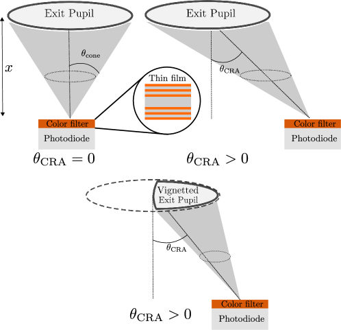
Figure 1: A schematic representation of how an aperture focuses light on the spectral imaging sensor with integrated thin-film optical filters. In the case of vignetting, part of the exit pupil is cut off. Only the vignetted exit pupil then contributes to focusing the light.

The imaging system used in this article consists of an objective lens with a finite aperture (exit pupil) which focuses the light onto pixels of an imaging sensor with integrated thin-film interference filters (Fig. 1). The output DN (Digital Number) of a pixel with integrated filters can be modeled as

$$\text{DN}=\int_{\lambda_{\mathrm{l}}}^{\lambda_{\mathrm{r}}}T(\lambda)\cdot L(\lambda)\,\textup{d}\lambda.$$ (1)

Here $L(\lambda)$ is the irradiance spectrum of the light incident at the pixel and $T(\lambda)$ is the transmittance of the filter measured under orthogonal collimated light conditions. The gain factors are assumed to be equal to 1 and are therefore omitted [7]. The limits of the integral describe the bandpass range of the spectral camera.

For a given f-number (characterized by half-cone angle $\theta_{\text{cone}}$) and chief ray angle $\theta_{\text{CRA}}$, the effect of the aperture and optical vignetting on the filter with central wavelength $\lambda_{\text{cwl}}$ is modeled as a convolution of $T(\lambda)$ with a kernel $K_{\theta_{\text{cone}},\,\theta_{\text{CRA}}}(\lambda)$ such that

$$\text{DN}=\int_{\lambda_{\mathrm{l}}}^{\lambda_{\mathrm{r}}}(K_{\theta_{\text{cone}},\,\theta_{\text{CRA}}}*T)(\lambda)\cdot L(\lambda)\,\textup{d}\lambda,$$ (2)

with $*$ being the convolution operator and the f-number being the ratio of the effective focal length to the diameter of the entrance pupil.

Below in Table 1, the most important symbols are summarized.

Table 1: List of the main symbols and their meaning.

Symbol	unit	Meaning
T($\lambda$)		Transmittance of a filter under
		orthogonal collimated conditions
$\lambda_{\text{cwl}}$	nm	central wavelength of filter
$f_{\#}$		f-number
$f_{\#,W}$		working f-number
$x$	mm	distance from pixel to exit pupil plane
$d$	mm	distance from optical axis
$\theta_{\text{CRA}}$	rad	chief ray angle
$\theta_{\text{cone}}$	rad	half-cone angle of the image side
		light cone
$R$	mm	Radius of the circular exit pupil
$P$	mm	Radius of the projected vignetting circle
$h$	mm	Distance of exit pupil to entrance circle

2.2 Finite aperture correction

In spectral camera designs where interference filters are spatially arranged behind an objective lens, understanding the impact of focused light from a finite aperture becomes essential. In this section we discuss the effect of the angle of incidence on thin-film Fabry-Pérot filters and the main results of prior work on the effect of focused light.

Thin-film Fabry-Pérot filters are constructed by combining multiple layers of a high and a low refractive index material [8]. The filters approximate behavior of the ideal Fabry-Pérot etalon.

The transmittance characteristics of interference filters change with the angle of incidence of the light. The larger the angle of incidence, the more the transmittance peak shifts towards shorter wavelengths.

The angle-dependent behavior of multilayer thin-film filters can be simulated using the transfer-matrix method [8]. However, for angles up to 40 degrees it was shown that the filter can be modeled as an ideal Fabry-Pérot etalon [9, 8]. This idealized etalon has an effective cavity material with an effective refractive index $n_{\text{eff}}$ which depends on the materials used.

The shift in central wavelength of a thin-film Fabry-Pérot filter with effective refractive index $n_{\text{eff}}$ for an incident angle $\phi$ is well approximated by $\Delta(\phi)$ which is defined as

$$\Delta(\phi)=-\lambda_{\text{cwl}}\left(1-\sqrt{1-\dfrac{\sin^{2}\phi}{n_{\text{eff}}^{2}}}\right),$$ (3)

with $\lambda_{\text{cwl}}$ the central wavelength of the transmittance peak. We have changed the sign convention compared to Eq. (3) in [6]. It is natural to consider a negative shift because the central wavelength becomes shorter.

This shift in central wavelength can also be modeled as a convolution of the initial transmittance $T(\lambda)$ with a shifted Dirac distribution such that

$$T_{\phi}(\lambda)\sim T(\lambda)*\delta\left(\lambda-\Delta(\phi)\right).$$ (4)

To model the effect of a finite aperture, focused light can be interpreted as a distribution of incident angles characterized by two parameters: the cone angle $\theta_{\text{cone}}$ (or f-number) and chief ray angle $\theta_{\text{CRA}}$ (Fig. 1). The analysis can be simplified by decomposing the focused beam of light in contributions of equal angles of incidence. In earlier work we have shown that the effect of the aperture can be modeled by a convolution of the transmittance of the filter with a kernel $K_{\theta_{\text{cone}},\,\theta_{\text{CRA}}}(\lambda)$ [6]. The kernel was defined as

$$K_{\theta_{\text{cone}},\,\theta_{\text{CRA}}}(\lambda)\sim\dfrac{2\,n_{\text{eff}}^{2}}{\lambda_{\text{cwl}}}\cdot\dfrac{\displaystyle\eta\left(n_{\text{eff}}\sqrt{-\dfrac{2\lambda}{\lambda_{\text{cwl}}}}\right)}{\pi\tan^{2}\theta_{\text{cone}}},$$ (5)

as used in Eq. (2) and with $\eta$ as it will be defined in Eq. (15). The changes in the transmittance of the filters cause undesired shifts in the measured spectra.

Two differences to the corresponding Eq. (15) in [6] must be pointed out. First, because of the change in sign convention (see Eq. (3)), there is a sign difference under the square root sign. Second, in this equation, the symbol $\eta$ is equal to $\gamma$ as used in Eq. (15) in [6], where it was used for the case without vignetting. In this article, the symbol $\gamma$ will be reserved for the more general case of vignetting.

In prior work we showed that the mean value $\bar{\lambda}$ of the kernel can quantify the shift in central wavelength. The mean value of the kernel was asymptotically equivalent to

$$\bar{\lambda}\sim-\lambda_{\text{cwl}}\left(\dfrac{\theta_{\text{cone}}^{2}}{4n_{\text{eff}}^{2}}+\dfrac{\theta_{\text{CRA}}^{2}}{2n_{\text{eff}}^{2}}\right),\ \text{for }\theta_{\text{cone}},\theta_{\text{CRA}}\rightarrow 0.$$ (6)

This formula can be used to correct the measured spectra. The wavelength at which the response of each pixel is plotted is updated as

$$\lambda_{\text{cwl}}^{\text{new}}=\lambda_{\text{cwl}}+\bar{\lambda}=\lambda_{\text{cwl}}\left(1-\dfrac{\theta_{\text{cone}}^{2}}{4n_{\text{eff}}^{2}}-\dfrac{\theta_{\text{CRA}}^{2}}{2n_{\text{eff}}^{2}}\right).$$ (7)

In this article an important extension of the above analysis is presented. The model is generalized to include optical vignetting which is a common phenomenon in many real lenses.

2.3 Vignetting

Vignetting is the fall-off in intensity that is observed in an image that was taken of a uniformly illuminated scene. There are many types of vignetting that can occur simultaneously. Examples are the cosine-fourth fall-off, optical vignetting, mechanical vignetting, pixel vignetting and pupil aberrations.

The ’cosine-fourth’ fall-off, also called natural vignetting is an effect intrinsic to even ideal thin lenses. It is caused by projected areas of the lens and pixels and the inverse square law. It implies that, under certain assumptions, the intensity of the light will be scaled by a factor $\cos^{4}\theta_{\text{CRA}}$ [10]. In wide-angle lenses the effect is more pronounced and is often corrected for by design [11, 12].

Optical vignetting occurs due to the physical length of a lens system or the position of a limiting aperture somewhere in the optical path [12, 13]. In essence, lens elements can shade other lens elements (Fig. 2). This causes part of the light beam to be cut off. The amount of optical vignetting depends on the aperture size and is less pronounced for smaller apertures (high f-numbers).

Figure 2: Illustration of optical vignetting. The off-axis point does not receive light from the complete aperture stop (lens B). This optical vignetting is caused by the limited diameter of lens A, causing lens B to be partially shaded [12].

In mechanical vignetting part of the scene is externally obstructed by for example the lens hood. This can cause the entrance pupil to be partially shaded [13]. In the proposed model there will be no fundamental difference with optical vignetting.

Pixel vignetting is an effect in CMOS digital cameras where the photodiode is positioned at the end of a tunnel in the back end of line of the image sensor [14]. Light can only reach the photodiode via the tunnel which when illuminated at oblique incidence, casts a shadow on the photodiode. Pixel vignetting behaves similar to optical vignetting since it also cuts of part of the light beam.

Pupil aberrations describe how the aperture is not uniformly illuminated [15]. Other types of aberrations cause the exit pupil to move or change in size [16, 17].

In the remainder of this article it is assumed that optical and mechanical vignetting are the dominant effects. Unless when specified, we will use the term ’vignetting’ and ’vignetted aperture’ to imply optical and mechanical vignetting.

2.4 Modeling a vignetted aperture

A vignetted aperture is an aperture that is partially cut off as a result of optical or mechanical vignetting. This aperture will be seen as a differently shaped exit pupil for each pixel (Fig. 1). In this article the ’exit pupil’ is the image of the aperture stop (full circle) and the ’vignetted exit pupil’ is the part of the exit pupil still focuses light onto the pixel.

An insightful approach to understand the shape of a vignetted aperture is provided by the variable cone model [11]. This model assumes that there is one finite aperture (exit pupil) that is encapsulated in a tube with length $h$ and an entrance circle of radius $P$ (Fig. 3). It also assumes that the incident light is collimated.

The exit pupil is the image of the limiting aperture (aperture stop) somewhere in the lens system. The second most limiting aperture will be responsible for most of the vignetting. The image of this second aperture is modeled by the entrance circle of radius $P$ of the tube in Fig. 3. The projection of this entrance circle onto the plane of the exit pupil is called the projected vignetting circle.

Because of its physical dimensions, the tube casts a shadow onto the exit pupil plane. The part of the exit pupil that still contributes to focusing the light is then the intersection of the exit pupil and the projected vignetting circle (red area in Fig. 3). This remaining part we will call the ’vignetted exit pupil’.

The assumption of collimated light simplifies the analysis. In real lens systems however, the light might not be collimated. Yet, even in these cases the exit pupil is still cut off by some circle [12]. The assumption will therefore only impact the fitted values for $P$ and $h$.

Figure 3: Optical vignetting is modeled with a finite aperture (exit pupil) encapsulated in a tube illuminated with collimated light. The tube has an opening of radius $P$ at a distance $h$. The vignetted exit pupil is the overlapping area between the exit pupil and the projected vignetting circle. Only the vignetted exit pupil still focuses light.

To calculate the shape of the vignetted exit pupil, the distances $d$ and $d_{v}$ need to be defined (Fig. 3). The position of a pixel $d$ is characterized by the distance to the optical axis such that

$$d=x\tan\theta_{\text{CRA}}.$$ (8)

The position $d_{v}$ of the center of the projected vignetting circle

$$d_{v}=h\tan\theta_{\text{CRA}}.$$ (9)

From Eq. (8) and Eq. (9) it follows that the relative size of $h$ and $x$ causes qualitative differences. This is discussed in the next section.

The variable cone model offers useful intuition about the behavior of optical vignetting. The larger the radius $P$ relative to $R$, the larger $d_{v}$ (and hence $\theta_{\text{CRA}}$) needs to become before part of the exit pupil is cut off. This intuitively explains why for smaller apertures (small R), there is less optical vignetting.

The variable cone model has been used before to model the intensity fall off. However, it has never been used to calculate the distribution of incident angles. Therefore, in the next section, we calculate how the shape of the vignetted exit pupil changes the distribution of incident angles for each pixel. We then calculate how this distribution impacts the transmittance of the integrated thin-film Fabry-Pérot filters.

2.5 Focused light from a vignetted aperture

Each filter has a transmittance $T(\lambda)$ when illuminated under orthogonal, collimated conditions. When used with a lens, and because of vignetting, each filter on the sensor array sees a different distribution of incident angles. The resulting transmittance is defined as $\hat{T}_{\theta_{\text{cone}},\,\theta_{\text{CRA}}}(\lambda)$.

To analyze the focused light beam from the vignetted aperture, the light beam can be decomposed in contributions of equal angle of incidence $\phi$ (Fig. 4). Each contribution can then be treated separately using the tilt angle model from Eq. (4).

The resulting transmittance is a linear combination of contributions of the form of Eq. (4), each representing a different angle of incidence. The weight of each contribution is the infinitesimal area $\textup{d}A$ of the aperture that contributes to the same angle of incidence $\phi$ (marked by blue in Fig. 4). The transmittance thus becomes

$$\hat{T}_{\theta_{\text{cone}},\,\theta_{\text{CRA}}}(\lambda)=\dfrac{\displaystyle\iint\limits_{\tiny\begin{subarray}{c}\text{Vignetted}\\ \text{exit pupil}\end{subarray}}T_{\phi}(\lambda)\,\textup{d}A}{\displaystyle\iint\limits_{\tiny\begin{subarray}{c}\text{Vignetted}\\ \text{exit pupil}\end{subarray}}\,\textup{d}A},$$ (10)

where the normalization is required because of conservation of energy.

Figure 4: For each $\theta_{\text{CRA}}$, the light beam is decomposed in contributions with equal angles of incidence. The weight of a contribution is measured by the length of the blue arc within the aperture. Parts of the blue arc can be cut off by the projected vignetting circle.

Because of linearity of the operators, $\hat{T}_{\theta_{\text{cone}},\,\theta_{\text{CRA}}}(\lambda)$ can be written as a convolution of the transmittance $T(\lambda)$ at orthogonal collimated conditions with a kernel $K_{\theta_{\text{cone}},\,\theta_{\text{CRA}}}(\lambda)$ such that

$$\hat{T}_{\theta_{\text{cone}},\,\theta_{\text{CRA}}}(\lambda) = T(\lambda)*\dfrac{\displaystyle\iint\limits_{\tiny\begin{subarray}{c}\text{Vignetted}\\ \text{exit pupil}\end{subarray}}\delta(\lambda-\Delta(\phi))\,\textup{d}A}{\displaystyle\iint\limits_{\tiny\begin{subarray}{c}\text{Vignetted}\\ \text{exit pupil}\end{subarray}}\,\textup{d}A}$$ (11)

$$= T(\lambda)*\dfrac{\displaystyle\iint\limits_{\tiny\begin{subarray}{c}\text{Vignetted}\\ \text{exit pupil}\end{subarray}}\delta(\lambda-\Delta(\phi))\,\textup{d}A}{A(\theta_{\text{cone}},\theta_{\text{CRA}})}$$ (12)

$$= T(\lambda)*K_{\theta_{\text{cone}},\,\theta_{\text{CRA}}}(\lambda).$$ (13)

Here $A(\theta_{\text{cone}},\theta_{\text{CRA}})$ is the area of the exit pupil which, because of vignetting, also changes with the chief ray angle (see Appendix A).

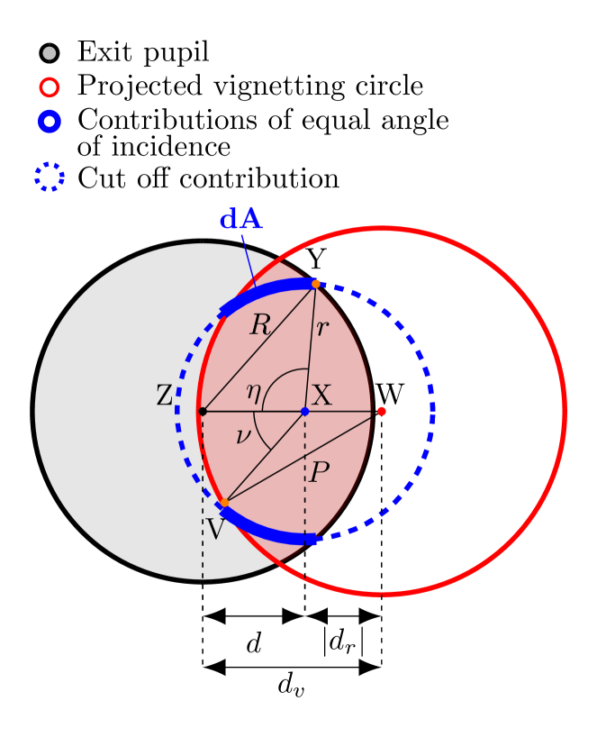
(a) Top view of the exit pupil plane for $h\geq x$ or equivalently $d_{v}\geq d$. A part of the contributions of equal angle of incidence is cut off so that only the thick blue line remains.

(b) Top view of the exit pupil plane for $h<x$ or equivalently $d_{v}<d$. The part cut off by the vignetting circle is qualitatively different than in Fig. 5(a).

Figure 5: Decomposition of the light cone from the aperture in contributions of equal angle of incidence $\phi$. The weight of each contribution is the infinitesimal area $\,\textup{d}A$ (blue). Here $d$ is the distance to the pixel from the optical axis.

The set of all possible rays that have the same incident angle on a pixel is a hollow cone with half-cone angle $\phi$ (the blue cone in Fig. 4). The intersection of this cone with the exit pupil plane is a circle with radius $r=x\tan\phi$.

In reality there are only rays coming from within the exit pupil. This subset is the part of the blue circle that lies within the exit pupil (Fig. 4). Its contribution is calculated as the infinitesimal area $\textup{d}A$ of a ring segment (Fig. 5(a)):

$$\textup{d}A=2\gamma(\arctan\dfrac{r}{x})r\textup{d}r=2\gamma(\phi)r\textup{d}r,$$ (14)

with $\gamma(\phi)$ being the angle of the arc within the exit pupil that contributes to the same angle of incidence $\phi=\arctan\frac{r}{x}$.

The angle $\gamma$ will be defined as a function of two other angles: $\eta$ and $\nu$. The angle $\eta$ is the angle that describes the contribution in the absence of vignetting (Fig. 5(a)). It is only limited by the area of the exit pupil. The effect of vignetting will be that only a subsection of the arc described by $\eta$ will be relevant. This relevant part is calculated using the angle $\nu$. It is the angle that describes what part of the arc is cut off (Fig. 5(a)) or kept (Fig. 5(b)) by the vignetting circle.

Taking into account that $r=x\tan\phi$, the angle $\eta(\phi)$ is determined by the law of cosines in $\Delta\text{XYZ}$ (Fig. 5(a)) as

$$\eta(\phi)=\text{Re}\left(\textup{arccos}\dfrac{d^{2}-R^{2}+r^{2}}{2dr}\right).$$ (15)

By taking the real part of the inverse cosine, the case in which there is a complete contributing circle within the aperture is also modeled (Fig. 4) [6]. This is because $\text{Re}(\arccos z)=\pi,\,\text{for}\,z\leq-1$.

Similarly, $\nu(\phi)$ is defined by applying the law of cosines in $\Delta\text{XWV}$ (Fig. 5) such that for $h\geq x$,

$$\nu(\phi)=\pi-\text{Re}\left(\textup{arccos}\dfrac{d_{r}^{2}-P^{2}+r^{2}}{2|d_{r}|r}\right).$$ (16)

By defining $d_{r}=d-d_{v}$, the above expression can be simplified as

$$\nu(\phi)=\text{Re}\left(\textup{arccos}\dfrac{d_{r}^{2}-P^{2}+r^{2}}{2d_{r}r}\right),$$ (17)

which covers both $h\geq x$ and $h<x$.

From these definitions and Fig. 5(a) it follows that the resulting contributing arc is defined as

$$\gamma(\phi)=\begin{cases}\max(\eta(\phi)-\nu(\phi),0)&h\geq x\\ \min(\eta(\phi),\nu(\phi))&h<x\end{cases},$$ (18)

where $\nu(\phi)$ is the angle that is either cut off or kept, depending on the relative size of $h$ and $x$. In the case $h\geq x$, $\nu$ represents the angle that is cut off by the vignetting circle (Fig. 5(a)). Therefore it must be subtracted from $\eta$. The $\max$ operator is needed because there is either a positive contribution or no contribution. A negative angle for $\gamma$ has no physical meaning.

In the case $h<x$, $\nu$ represents the angle of the arc that is not cut off (Fig. 5(b)). This is modeled by taking the mininum of $\eta$ and $\nu$.

To work with the angle of incidence $\phi$, $r$ is substituted with $r=x\tan\phi$ such that

$$\textup{d}A=2x^{2}\gamma(\phi)\dfrac{\tan\phi}{\cos^{2}\phi}\textup{d}\phi.$$ (19)

The integral then becomes

$$K_{\theta_{\text{cone}},\,\theta_{\text{CRA}}}(\lambda)=\dfrac{\displaystyle\int_{\phi_{\text{min}}}^{\phi_{\text{max}}}2x^{2}\gamma(\phi)\dfrac{\tan\phi}{\cos^{2}\phi}\delta(\lambda-\Delta(\phi))\,\textup{d}\phi}{A(\theta_{\text{cone}},\theta_{\text{CRA}})}.$$ (20)

Here $\phi_{\text{min}}$ and $\phi_{\text{max}}$ are the smallest and largest incident angles coming from the aperture (See Appendix B).

An asymptotic approximation of the kernel is

$$K_{\theta_{\text{cone}},\,\theta_{\text{CRA}}}(\lambda)\sim\displaystyle\frac{2\,n_{\text{eff}}^{2}}{\lambda_{\text{cwl}}}\cdot\dfrac{\gamma\left(n_{\text{eff}}\sqrt{-\dfrac{2\lambda}{\lambda_{\text{cwl}}}}\right)}{A(\theta_{\text{cone}},\theta_{\text{CRA}})}x^{2},$$ (21)

as used in Eq. (2). For the derivation see Appendix A.

Initially, the kernel in Eq. (21) is equivalent to the kernel in the ideal finite aperture case (Eq. (5)). After the onset of vignetting, the kernel is cut-off (Fig. 6). Because the kernel is less wide, the resulting transmittance will be shifted less. In the next section we derive how to calculate this shift.

Figure 6: The shape of the kernel is qualitatively shown for different regimes of $\theta_{\text{CRA}}$ and $\theta_{\text{cone}}$. Vignetting causes the kernel to be cut off. The dotted line continues the shape of the kernel in the absence of vignetting.

2.6 Wavelength correction method

Each filter has been designed to sense a specific wavelength. This wavelength is defined as the central wavelength $\lambda_{\text{cwl}}$ of the transmittance when illuminated in orthogonal collimated conditions. To plot the spectrum, the response for each filter is plotted at this central wavelength $\lambda_{\text{cwl}}$.

As discussed however, the actual central wavelength of the filter depends on the angular distribution of the incident light. Thus, to correctly plot a spectrum, the central wavelength needs to be corrected for each filter, taking its physical position into account.

The shift in central wavelength can be quantified by the mean of the kernel (when interpreted as a distribution) [6]. The mean is defined as

$$\bar{\lambda}_{\theta_{\text{cone}},\,\theta_{\text{CRA}}} = \dfrac{\displaystyle\int_{\lambda_{\text{min}}}^{\lambda_{\text{max}}}\lambda K_{\theta_{\text{cone}},\,\theta_{\text{CRA}}}(\lambda)\,\textup{d}\lambda}{\displaystyle\int_{\lambda_{\text{min}}}^{\lambda_{\text{max}}}K_{\theta_{\text{cone}},\,\theta_{\text{CRA}}}(\lambda)\,\textup{d}\lambda}$$ (22)

$$\stackrel{{\scriptstyle\tiny\tiny\text{(normalized)}}}{{=}} \displaystyle\int_{\lambda_{\text{min}}}^{\lambda_{\text{max}}}\lambda K_{\theta_{\text{cone}},\,\theta_{\text{CRA}}}(\lambda)\,\textup{d}\lambda.$$

In Appendix B we explain how to numerically approximate this integral.

To calculate the new central wavelength of the filter the mean value $\bar{\lambda}$ is added to the original central wavelength such that

$$\lambda_{\text{cwl}}^{\text{new}} = \lambda_{\text{cwl}}+\bar{\lambda}_{\theta_{\text{cone}},\,\theta_{\text{CRA}}}.$$ (23)

The negative mean value is added because the shifts are towards shorter wavelengths.

2.7 Model parameter estimation

In this section a practical algorithm is presented to estimate the model parameters based on the vignetting profile.

The vignetting profile can be measured by illuminating the entrance pupil uniformly with diffuse light from an integrating sphere.

The vignetting profile does not only describe optical vignetting. Natural vignetting, pixel vignetting and pupil aberrations might also be present. An algorithm is therefore required to isolate the contribution of optical and mechanical vignetting.

Optical vignetting is characterized by an abrupt change in the vignetting profile [11]. This abrupt change is caused by the vignetting circle which suddenly starts cutting off part of the exit pupil. This discontinuity can be exploited to isolate optical vignetting from other contributions to the intensity fall-off.

The onset of optical vignetting is when the vignetting circle just touches the border of the aperture. This happens when the the vignetting circle has moved a distance equal to the difference in radii such that

$$d_{v}=P-R.$$ (24)

Rearranging gives

$$P-d_{v}=P-h\tan\theta_{\text{CRA}}=R=x\tan\theta_{\text{cone}}.$$ (25)

For each vignetting profile measured at a different f-number, an equation of the form of Eq. (25) can be written down. The corresponding chief ray angles are obtained from the vignetting profile at the point where the abrupt change starts.

The unknown model parameters $P$ and $h$ can then be estimated from solving the (possibly overdetermined) linear system

$$\begin{bmatrix}1&-\tan(\theta_{\text{CRA},1})\\ \vdots&\vdots\\ 1&-\tan(\theta_{\text{CRA},n})\\ \end{bmatrix}\begin{pmatrix}P\\ h\end{pmatrix}=\begin{pmatrix}R_{1}\\ \vdots\\ R_{n}\end{pmatrix}.$$ (26)

To determine the radius $R$ of the exit pupil, the working f-number $f_{\#,W}$ must be used. The working f-number is calculated as ([18])

$$f_{\#,W}\approx\left(1+\frac{m}{m_{P}}\right)f_{\#},$$ (27)

with $m$ and $m_{P}$ being the linear and pupil magnification respectively.

The definition of the f-number then implies that

$$R=x\tan\theta_{\text{cone}}=\dfrac{x}{2f_{\#,W}}.$$ (28)

3 Experimental validation

In this section, we estimate the model parameters and demonstrate that using Eq. (23) the shifted spectra in measurements can be corrected.

3.1 Experimental setup

We make use of Imec’s VNIR Snapscan camera [19]. In the Snapscan the image sensor is placed behind the lens and its position can be controlled using an automated translation stage. This makes the system ideally suited for controlling the chief ray angles. The Snapscan is used with an Edmund Optics 16 mm C Series VIS-NIR fixed focal length lens because it has large chief ray angles and has considerable vignetting.

To efficiently compare different points in the scene, a color filter was placed in front of the lens. The scene was filled with a uniform white reference tile (Fig. 7(a)). The combination of the filter and white reference effectively creates a scene-filling uniform spectral target.

The transmittance of the color filter is calculated using a flat-fielding approach. This requires taking three images: a dark image (no light) and two images of the white reference tile, one with and one without color filter. Using the notation of the spectral imaging model (Eq. (2)), the transmittance is then calculated as

$$\text{transmittance}=\dfrac{\text{DN}_{\text{filter}}-\text{DN}_{\text{dark}}}{\text{DN}_{\text{white}}-\text{DN}_{\text{dark}}}.$$ (29)

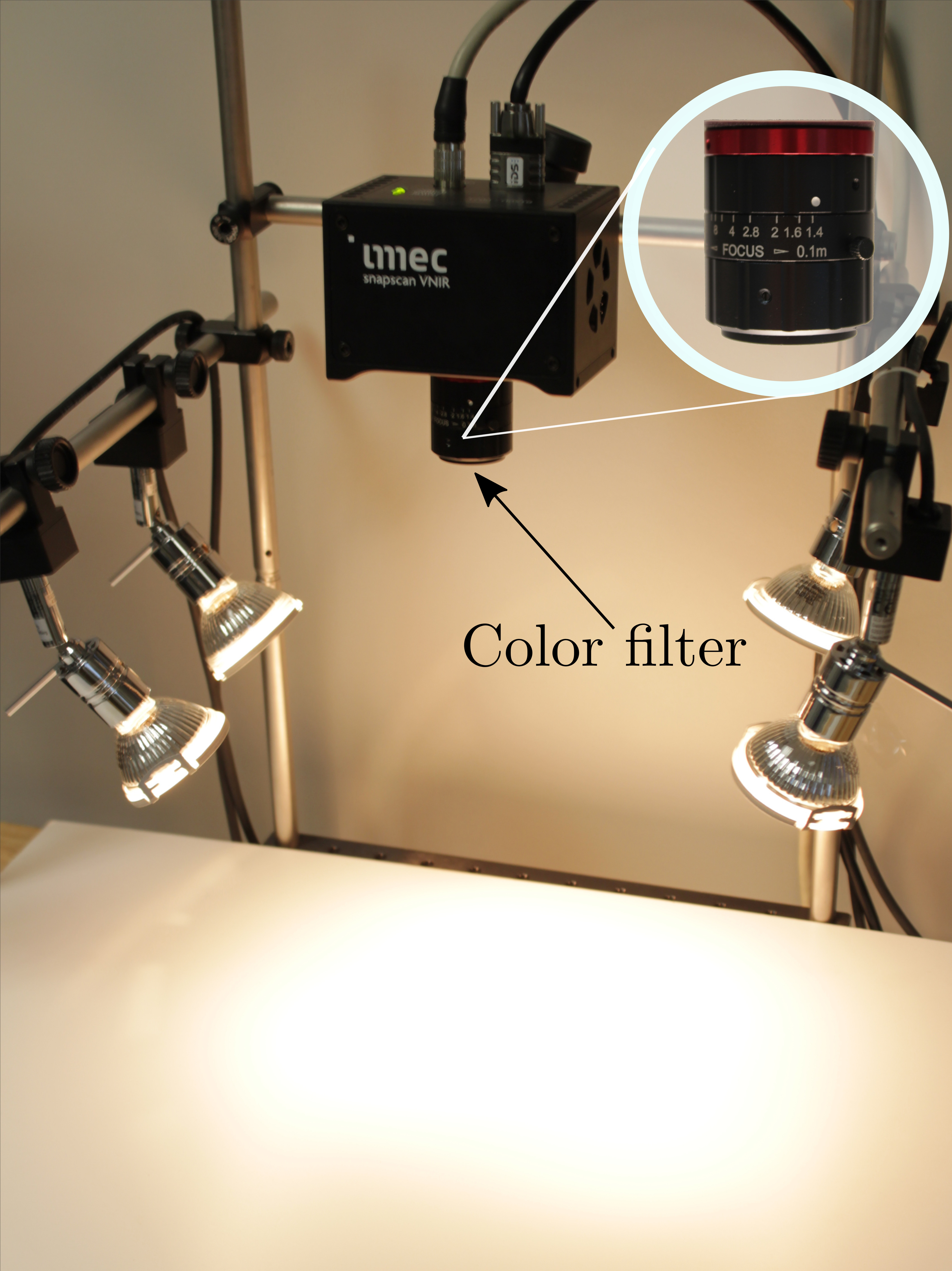
(a) Imec’s Visible Near-Infrared Snapscan camera.

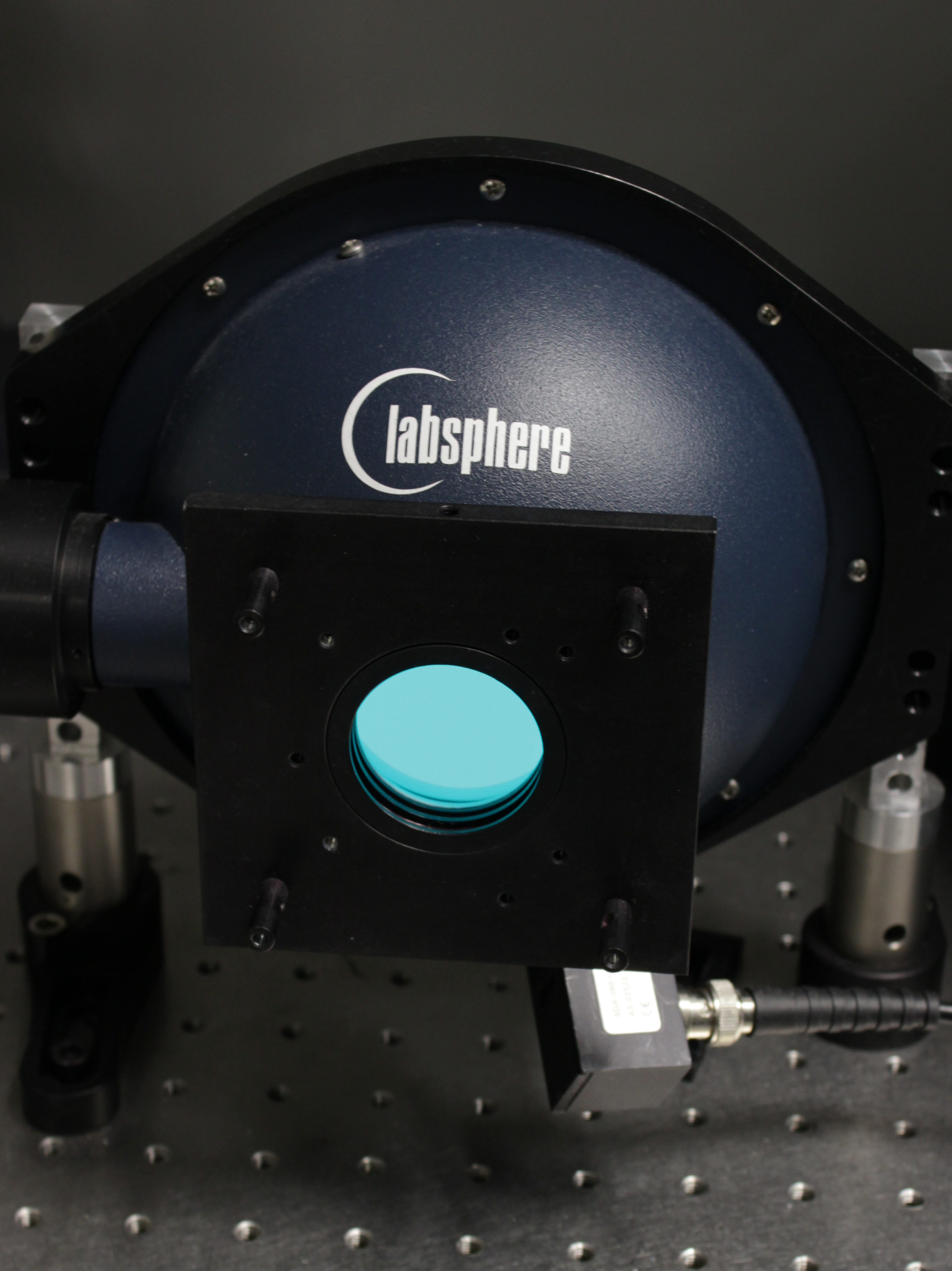
(b) Integrating sphere to measure vignetting profiles.

Figure 7: Experimental setups.

The Edmund Optics 16 mm lens is focused at the target surface (approx. 24 mm from the lens).

3.2 Model parameter estimation

We apply the model parameter estimation method from Eq. (26) to an Edmund Optics 16 mm lens. The exit pupil $x=21\,\text{mm}$, linear magnification $m=0.06$ and pupil magnification $m_{P}=1.3$. The filters have an effective refractive index of $n_{\text{eff}}=1.7$.

The vignetting fall-off profiles were measured using a camera with a panchromatic image sensor. The camera was illuminated with uniform light from an integrating sphere (Fig. 7(b)). In the vignetting profiles there are several discontinuities, marked by black dots in Fig. 8. To isolate the discontinuities in the vignetting profile we found that they are best visualized when the vignetting profile is divided by the profile measured for a high f-number (Fig. 8). Since for this high f-number there is no optical vignetting, this approach seems to cancel out some of the other contributions. This operation is merely for visualization purposes and does not impact the fitting procedure since the position of the discontinuities remain unchanged.

From Fig. 8 and Eq. (26) it follows that the following overdetermined system must be solved:

$$\begin{bmatrix}1&-\tan(0.38^{\circ})\\ 1&-\tan(9^{\circ})\\ 1&-\tan(13^{\circ})\\ 1&-\tan(15.4^{\circ})\end{bmatrix}\begin{pmatrix}P\\ h\end{pmatrix}=\begin{pmatrix}7.1715\\ 5.0201\\ 3.5858\\ 2.5100\end{pmatrix}.$$ (30)

Where each angle corresponds to a black dot on Fig. 8. And $R_{i}$ was determined using Eq. (28).

The solution of the overdetermined system, using the Moore–Penrose inverse, is

$$\begin{pmatrix}P\\ h\end{pmatrix}=\begin{pmatrix}7.4236\\ 16.991\end{pmatrix}.$$ (31)

We are in the $h<x$ regime because $16.99<21$ mm.

The deviations from the model prediction mean that there are other effects that contribute to the vignetting profile. Nevertheless, the onset of vignetting, as marked by the black dots, can be predicted very well. The deviations might be due to the fact that natural vignetting changes with the aperture size [10] or because of pupil aberrations. However, as we will see in the results, these deviations have little impact on the correction of the shifted spectra.

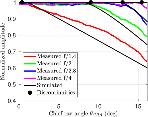
Figure 8: Vignetting profile for Edmund Optics 16 mm lens measured for different f-numbers. Using the estimated model parameters from Eq. (31), the vignetting profile is predicted (black line).

3.3 Experiment and data analysis

In each experiment, transmittance images (Eq. (29)) are taken at different f-numbers using the setup shown in Fig. 7(a). For each f-number, the spectrum is plotted at three chosen positions that correspond to chief ray angles of $1.9^{\circ}$, $10.3^{\circ}$ and $17.4^{\circ}$.

To plot the spectra, the output (Eq. (29)) for each pixel is plotted at the original central wavelength $\lambda_{\text{cwl}}$ of the deposited filter. Because of this, the shifts of the filters towards shorter wavelengths creates the illusion that the spectra move towards longer wavelengths. The actual spectrum of the incident light, of course, does not change.

We plot three graphs. The first is the uncorrected transmittance for all the samples. The second is the transmittance corrected assuming an ideal finite aperture (Eq. (7)). The third is the transmittance corrected using the vignetting model (Eq. (23)).

For comparison, we also simulate the results of the experiment. The simulation is done by combining Eq. (2) and Eq. (29).

For each plot we also display two metrics that quantify the improvement: the correlation coefficient and the maximum error. These quantities were calculated for each pair of spectra. Only the worst values are displayed on the graph.

3.4 Results

The uncorrected transmittances show clear variations compared to the reference measured at $f/8$ (Fig. 9(a)). The variations are plotted for each f-number separately in (Fig. 10)

The different spectra measured at $f/1.4$ are shifted less compared to the higher f-numbers (Fig. 10). Intuitively one would expect larger deviations for smaller f-numbers. Without vignetting at $f/1.4$, the spread between the measured spectra for filters centered at 700 nm should be about 11 nm while the measured spread is about 2 nm.

Therefore, if one ignores the presence of optical vignetting and uses Eq. (7) to correct the central wavelengths, the shifts are significantly overcorrected (Fig. 9(b) and 10(b)). Because optical vignetting is more pronounced for smaller f-numbers, these are overcorrected the most.

If the vignetting model is used to correct the central wavelengths using Eq. (23), the different spectra align very well, as desired (Fig. 9(c)).

In the simulation, very similar results are obtained (Fig. 11). This shows that the model can also be used to predict the impact of a lens with optical vignetting on the measurements. It also shows that even in simulation some variation remains after correction (Fig. 11(c)). This is because the kernel does not only shift the filters but also changes their shape (Fig. 6).

The differences between Fig. 9(b) and Fig. 9(c) can be better understood by comparing $Eq.\eqref{eq:idealmean}$ and $Eq.\eqref{eq:expectedvalue}$ visually (Fig. 12). This figure summarizes the effect of vignetting on the shift of the filters. It shows that after the onset of vignetting, Eq. (6) starts to overestimate the shift. The near constant value of the red curve also explains why the spread in shift for $f/1.4$ is only about 2 nm.

(a) Measured transmittance (uncorrected)

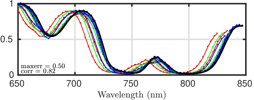
(b) Corrected using Eq. (7)

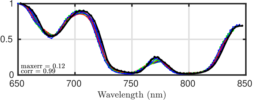
(c) Corrected using vignetting model Eq. (23)

Figure 9: Edmund Optics 16 mm lens. The uncorrected reflectance values demonstrate position and f-number dependent shifts. The spectrum is plotted at three chosen positions that correspond to chief ray angles of $1.9^{\circ}$, $10.3^{\circ}$ and $17.4^{\circ}$. Without considering vignetting, the model overcorrects the shifts (Fig. 9(b)). Using Eq. (23) with the estimated model parameters, the correction is significantly improved.

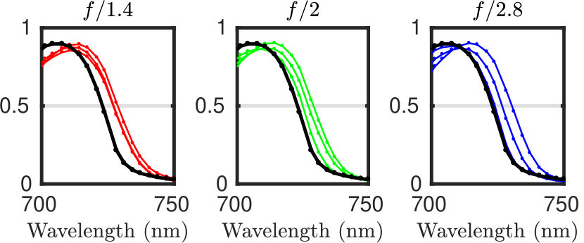
(a) Measured transmittance (uncorrected)

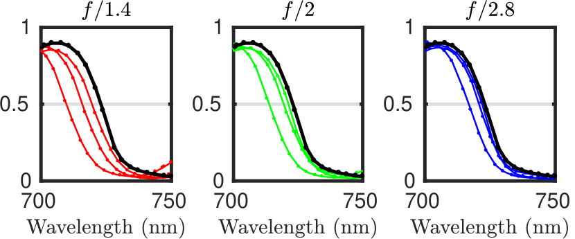
(b) Corrected using Eq. (7)

Figure 10: Close-up of a region in Fig. 9 for each separate f-number. The spread of the spectra for $f/1.4$ is smaller than for larger f-numbers. The correction with Eq. (23) is not shown here.

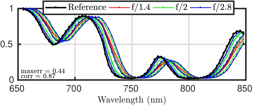
(a) Measured transmittance (uncorrected)

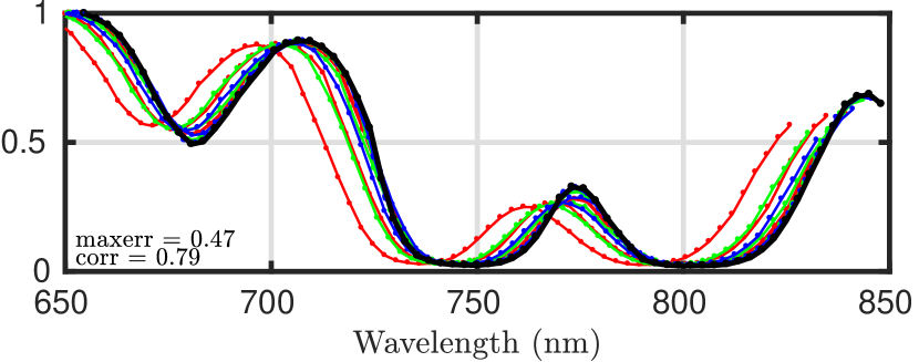
(b) Corrected using Eq. (7)

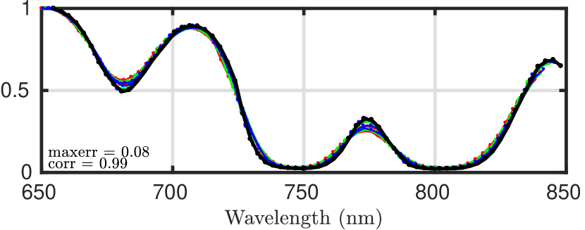
(c) Corrected using vignetting model Eq. (23)

Figure 11: Simulated Edmund Optics 16 mm lens. This is a simulation of the experimental conditions of Fig. 9. The shifts in the uncorrected and corrected spectra (Eq. (23)) are nearly identical to the real measurements.

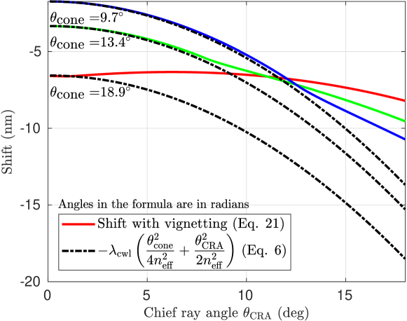
Figure 12: Numerical approximation of the mean value compared to the asymptotic approximation Eq. (6). The asymptotic approximation remains valid until the onset of optical vignetting. Simulated for $\lambda_{\text{cwl}}=700$ nm at f-numbers $f/1.4$ (red), $f/2$ (green) and $f/2.8$ (blue).

4 Discussion

The results demonstrate that the proposed method can be used to correct undesired shifts in measurements in the presence of optical or mechanical vignetting.

Correcting these position-dependent shifts is important for improving the performance of machine learning applications. And because vignetting is a common phenomenon, our method will be relevant for many practical applications.

The method is powerful since it can treat a lens as a black-box. This is important since often a complete physical model of the lens is unavailable. But even when a full model is available, it is still unpractical to get an idea of the dominant effects and how to correct for them. Our method offers a very practical way to isolate the effect of optical vignetting and estimate the model parameters to predict and correct it.

To make the effect of optical vignetting more understandable, more analytical studies on the subject are needed. Currently, the mean of the kernel is calculated numerically. An analytical approximation of the mean in the vignetting regime would be useful for intuitive understanding and quick calculations.

The vignetting model presented in this paper successfully generalizes the model from prior work [6]. However, the model also has some potential limitations which are discussed below.

First, there is the assumption that the vignetting circle moves proportional to $\tan\theta_{\text{CRA}}$ (Eq. (9)). This might not be a good approximation for some lenses. The equation however can be easily substituted without major changes to the correction method.

Second, pupil aberrations might cause changes in the radii of the exit pupil and projected vignetting circle. Pupil aberrations will be the topic of future work.

Third, theoretically there can multiple projected vignetting circles simultaneously present in the system. This means that the aperture is cut off in more complex ways. One example is pixel vignetting, which also limits the cone of light that can reach the photodiode. This effect was not studied in this article. However, in Fig. 8, for f/1.4, there is arguably a second discontinuity around $\theta_{\text{CRA}}\approx 11^{\circ}$. The extension to multiple vignetting circles could be investigated further. However, in our experiments the additional gains would be negligible.

5 Conclusion

In many applications it is important that the measured spectra are independent of the lens and the position of the target in the scene.

Shifts in the measured spectra are caused by the sensitivity of the filters to the angle of incidence and must be corrected for. In previous work we demonstrated this for real lenses that exhibited no vignetting.

Vignetting, however, is a common phenomenon in real lenses and must be taken into account for accurate correction. Thus, in this article we generalized our model for a vignetted aperture. We demonstrated that this generalization is vital for correcting the observed shifts in measured spectra.

Because vignetting is so common, our method has the potential to improve the performance of many spectral imaging applications. These will mostly be applications that use fast lenses (large aperture) or low cost lenses but still require high spectral accuracy.

Appendix

Appendix A Closed-form solution of the kernel

In this section we derive a closed-form solution of the kernel and derive the analytical approximation given in Eq. (21).

The derivation of the closed-form solution is identical to derivation presented in prior work (see [6]) up to a few minor modifications. First, the shape of the exit pupil changes and therefore also the distribution of incident angles. Thus $\gamma$ is defined by Eq. (18) instead of $\gamma(\phi)=\eta(\phi)$. Second, the area of the vignetted exit pupil changes. Therefore the kernel should be normalized accordingly. Therefore

$$\begin{array}[]{lcl}K_{\theta_{\text{cone}},\,\theta_{\text{CRA}}}(\lambda)&=&\dfrac{\displaystyle\int_{\phi_{\text{min}}}^{\phi_{\text{max}}}2x^{2}\gamma(\phi)\dfrac{\tan\phi}{\cos^{2}\phi}\delta(\lambda-\Delta(\phi))\,\textup{d}\phi}{\displaystyle\iint\limits_{\tiny\begin{subarray}{c}\text{Vignetted}\\ \text{exit pupil}\end{subarray}}\,\textup{d}A},\\ &=&\dfrac{\displaystyle\int_{\phi_{\text{min}}}^{\phi_{\text{max}}}2x^{2}\gamma(\phi)\dfrac{\tan\phi}{\cos^{2}\phi}\delta(\lambda-\Delta(\phi))\,\textup{d}\phi}{A(\theta_{\text{cone}},\theta_{\text{CRA}})},\\ \end{array}$$ (32)

with $\Delta(\phi)$ defined in Eq. (3) and $A(\theta_{\text{cone}},\theta_{\text{CRA}})$ being the area of the vignetted exit pupil which is defined as [11]

$$A(\theta_{\text{cone}},\theta_{\text{CRA}})=P^{2}(\alpha-\sin(\alpha)\cos(\alpha))+R^{2}(\beta-\sin(\beta)\cos(\beta)),$$ (33)

with

$$\alpha = \text{Re}\left(\arccos\dfrac{P^{2}-R^{2}+d_{v}^{2}}{2Pd_{v}}\right)$$ (34)

$$\beta = \text{Re}\left(\arccos\dfrac{R^{2}-P^{2}+d_{v}^{2}}{2Rd_{v}}\right),$$ (35)

and $d_{v}=h\tan\theta_{\text{CRA}}$ and $R=x\tan\theta_{\text{cone}}$.

The integral in Eq. (32) can be rewritten using the Heaviside function $H(\cdot)$. If we define $\Pi(\phi)=H(\phi-\phi_{\text{min}})-H(\phi-\phi_{\text{max}})$, then

$$\begin{array}[]{lcl}K_{\theta_{\text{cone}},\,\theta_{\text{CRA}}}(\lambda)&=&\dfrac{\displaystyle\int_{-\infty}^{\infty}2x^{2}\gamma(\phi)\dfrac{\tan\phi}{\cos^{2}\phi}\delta(\lambda-\Delta(\phi))\Pi(\phi)\,\textup{d}\phi}{A(\theta_{\text{cone}},\theta_{\text{CRA}})}.\end{array}$$ (36)

To proceed we use the same steps as described in Appendix A of [6], the only difference being the difference in sign convention for shift. The closed-form analytical solution to Eq. (36) can be formulated as

$$K_{\theta_{\text{cone}},\theta_{\text{CRA}}}(\lambda)=\dfrac{g(\lambda)\gamma(\Delta^{-1}(\lambda))}{A(\theta_{\text{cone}},\theta_{\text{CRA}})}x^{2}\Pi\left(\Delta^{-1}(\lambda)\right),$$ (37)

with $\gamma$ as defined in Eq. (18) and the function $g(\lambda)$ containing all remaining terms:

$$g(\lambda) = \dfrac{2n_{\text{eff}}^{2}}{\lambda_{\text{cwl}}}\cdot\dfrac{\left(1+\dfrac{\lambda}{\lambda_{\text{cwl}}}\right)}{\left(1+2n_{\text{eff}}^{2}\dfrac{\lambda}{\lambda_{\text{cwl}}}+n_{\text{eff}}^{2}\dfrac{\lambda^{2}}{\lambda_{\text{cwl}}^{2}}\right)^{2}}$$ (38)

$$= \frac{2\,n_{\text{eff}}^{2}}{\lambda_{\text{cwl}}}+\mathcal{O}\left(\dfrac{\lambda}{\lambda_{\text{cwl}}}\right),\quad\text{for }\dfrac{\lambda}{\lambda_{\text{cwl}}}\rightarrow 0.$$ (39)

The notation $\mathcal{O}(\cdot)$ is the Big O notation which describes the limiting behavior of the error term of the approximation.

Combining the approximation in Eq. (38) with

$$\begin{array}[]{l}\Delta^{-1}(\lambda)=\arcsin\left(n_{\text{eff}}\sqrt{-\dfrac{\lambda}{\lambda_{\text{cwl}}}\left(2+\dfrac{\lambda}{\lambda_{\text{cwl}}}\right)}\right)\\ =n_{\text{eff}}\sqrt{-\dfrac{2\lambda}{\lambda_{\text{cwl}}}}+\mathcal{O}\left(\dfrac{\lambda^{3/2}}{\lambda_{\text{cwl}}^{3/2}}\right),\quad\text{for }\dfrac{\lambda}{\lambda_{\text{cwl}}}\rightarrow 0,\end{array}$$ (40)

the kernel can be approximated as

$$K_{\theta_{\text{cone}},\,\theta_{\text{CRA}}}(\lambda)\sim\dfrac{2\,n_{\text{eff}}^{2}}{\lambda_{\text{cwl}}}\cdot\dfrac{\displaystyle\gamma\left(n_{\text{eff}}\sqrt{-\dfrac{2\lambda}{\lambda_{\text{cwl}}}}\right)}{A(\theta_{\text{cone}},\theta_{\text{CRA}})}x^{2}.$$ (41)

The only difference with the result from earlier work (Eq. (21)) is the value of $\gamma$ and that the area of the vignetted exit pupil now also varies with $\theta_{\text{CRA}}$.

Appendix B Calculating the mean of the kernel

The mean $\bar{\lambda}$ is required in the central wavelength correction formula of Eq. (23). The mean is defined by the integral

$$\int_{\lambda_{\text{min}}}^{\lambda_{\text{max}}}\lambda K_{\theta_{\text{cone}},\,\theta_{\text{CRA}}}(\lambda)\,\textup{d}\lambda.$$ (42)

In this article we numerically approximated the mean value and used this value for correction. For this, the limits $\lambda_{\text{min}}$ and $\lambda_{\text{max}}$ of the integral need to be known. By construction $\gamma(\phi)$ becomes zero where needed (Eq. (18)). Because of this and the fact the shift is always less than or equal to zero, the upper limit can always be taken zero in numerical integration. Therefore $\lambda_{\text{max}}=0$.

The lower integration limit however should be known exactly since there is no theoretical limit to its negative value.

For each case, there are two options. The maximal radius is constrained by either the exit pupil or the projected vignetting circle. If it is constrained by the exit pupil, $r_{\text{max}}=R+d$. If it is constrained by the vignetting circle, the result depends on whether $h\geq x$ or $h<x$.

In the case that $h>x$, the kernel becomes zero if $\eta=\nu$. The maximal radius if found by equating Eq. (15) and Eq. (17) and solve to r such that

$$r=\pm\frac{\sqrt{(d-d_{r})[d(P^{2}-d_{r}^{2})+d_{r}(d^{2}-R^{2})]}}{d-d_{r}},$$ (43)

of which only the positive solution is meaningful. For $h<x$, the maximal radius is $r=P+d_{r}$.

The maximal radius $r_{\text{max}}$ for all cases can be formulated compactly as

$$r_{\text{max}}=\begin{cases}\min(R+d,P+d_{r})&h<x\\ \min\left(R+d,\frac{\sqrt{(d-d_{r})[d(P^{2}-d_{r}^{2})+d_{r}(d^{2}-R^{2})]}}{d-d_{r}}\right)&h\geq x\end{cases}.$$ (44)

The min function models that either the exit pupil or the projected vignetting circle is the limiting circle.

From $r_{\text{max}}$, the maximal incident angle $\phi_{\text{max}}$ can be calculated. By definition, $\phi_{\text{max}}=\arctan\dfrac{r_{\text{max}}}{x}$. And finally, using Eq. (3),

$$\lambda_{\text{min}}=\Delta(\phi_{\text{max}}).$$ (45)

Using the chosen integration limits, the solution is then approximated using a left Riemann sum. A step size = 0.01 nm was used.

However for small values of $\theta_{\text{cone}}$, the kernel will converge to a Dirac distribution. Therefore a much smaller step size might be required. Instead it is advised to use the asymptotic approximation Eq. (6). In the presence of optical vignetting the asymptotic approximation is valid for $d_{v}<P-R$. Or alternatively,

$$\theta_{\text{CRA}}<\arctan\dfrac{P-R}{h}.$$ (46)

This condition specifies the onset of vignetting, after which the numerical solution should be used. The numerical solution and the asymptotic approximation are both plotted in Fig. 12.

This method is implemented in Code 1. A usage example is given in Code 2.

References

- [1] P. Shippert, “Why Use Hyperspectral Imagery?” \JournalTitleEarth Science 70, 377–379 (2004).
- [2] G. Lu and B. Fei, “Medical hyperspectral imaging: a review.” \JournalTitleJournal of biomedical optics 19, 10901 (2014).
- [3] A. Gowen, C. O’Donnell, P. Cullen, G. Downey, and J. Frias, “Hyperspectral imaging – an emerging process analytical tool for food quality and safety control,” \JournalTitleTrends in Food Science & Technology 18, 590–598 (2007).
- [4] B. Geelen, N. Tack, and A. Lambrechts, “A compact snapshot multispectral imager with a monolithically integrated per-pixel filter mosaic,” \JournalTitleProc. SPIE 8974, 89740L (2014).
- [5] N. Tack, A. Lambrechts, P. Soussan, and L. Haspeslagh, “A compact, high-speed, and low-cost hyperspectral imager,” \JournalTitleProc. SPIE 8266, Silicon Photonics VII 32, 82660Q (2012).
- [6] T. Goossens, B. Geelen, J. Pichette, A. Lambrechts, and C. Van Hoof, “Finite aperture correction for spectral cameras with integrated thin-film Fabry-Perot filters,” \JournalTitleAppl. Opt. 57, 7539–7549 (2018).
- [7] J. R. Janesick, Photon transfer (SPIE press San Jose, 2007).
- [8] H. A. Macleod, Thin-film optical filters (CRC press, 2001).
- [9] C. R. Pidgeon and S. D. Smith, “Resolving Power of Multilayer Filters in Nonparallel Light,” \JournalTitleJournal of the Optical Society of America 54, 1459 (1964).
- [10] I. C. Gardner, “Validity of the cosine-fourth-power law of illumination,” \JournalTitleJournal of the National Bureau of Standards 39, 213–219 (1947).
- [11] N. Asada, A. Amano, and M. Baba, “Photometric calibration of zoom lens systems,” \JournalTitleProceedings - International Conference on Pattern Recognition 1, 186–190 (1996).
- [12] W. J. Smith, Modern Optical Engineering (2000).
- [13] S. F. Ray, Applied Photographic Optics: Lenses and Optical Systems for Photography, Film, Video, Electronic and Digital Imaging (Focal, 2002).
- [14] P. B. Catrysse and B. a. Wandell, “Optical efficiency of image sensor pixels.” \JournalTitleJournal of the Optical Society of America. A, Optics, image science, and vision 19, 1610–1620 (2002).
- [15] M. Aggarwal, H. Hua, and N. Ahuja, “On cosine-fourth and vignetting effects in real lenses,” \JournalTitleInternational Conference on Computer Vision 1, 472–479 (2001).
- [16] L. Hazra, “Introduction to Aberrations in Optical Imaging Systems by José Sasián,” \JournalTitleJournal of Optics 42, 293–294 (2013).
- [17] J. Sasian, “Interpretation of pupil aberrations in imaging systems,” \JournalTitleProc. SPIE 6342, 6342 – 6342 – 4 (2006).
- [18] R. Kingslake, Optics in Photography, vol. 6 (SPIE Press Monograph, 1992).
- [19] J. Pichette, W. Charle, and A. Lambrechts, “Fast and compact internal scanning CMOS-based hyperspectral camera: the Snapscan,” \JournalTitleProc. SPIE 10110, 1011014 (2017).