Faraday instability on a sphere:
Floquet analysis

Abstract

Standing waves appear at the surface of a spherical viscous liquid drop subjected to radial parametric oscillation. This is the spherical analogue of the Faraday instability. Modifying the Kumar & Tuckerman (1994) planar solution to a spherical interface, we linearize the governing equations about the state of rest and solve the resulting equations by using a spherical harmonic decomposition for the angular dependence, spherical Bessel functions for the radial dependence, and a Floquet form for the temporal dependence. Although the inviscid problem can, like the planar case, be mapped exactly onto the Mathieu equation, the spherical geometry introduces additional terms into the analysis. The dependence of the threshold on viscosity is studied and scaling laws are found. It is shown that the spherical thresholds are similar to the planar infinite-depth thresholds, even for small wavenumbers for which the curvature is high. A representative time-dependent Floquet mode is displayed.

published in Journal of Fluid Mechanics 805, 591-610 (2016)

1 Introduction

The dynamics of oscillating drops are of interest to researchers in pattern formation and dynamical systems as well as having practical applications over a wide variety of scales, in areas as diverse as astroseismology, containerless material processing for high purity crystal growth and drug delivery and mixing in microfluidic devices.

Surface tension is responsible for the spherical shape of a drop. In the absence of external forces, if the drop is slightly perturbed, it will recover its spherical shape through decaying oscillations. This problem was first considered by Kelvin (1863) and Rayleigh (1879), who described natural oscillations of drops of inviscid fluids. Rayleigh (1879) and Lamb (1932) derived the now-classic resonance mode frequency resulting from the restoring force of surface tension:

$$\omega^{2}=\frac{\sigma}{\rho}\frac{\ell(\ell-1)(\ell+2)}{R^{3}}$$ (1)

where $\omega$ is the frequency, $\sigma$ and $\rho$ the surface tension and density, $R$ is the radius, and $\ell$ is the degree of the spherical harmonic

$$Y_{\ell}^{m}=P_{\ell}^{m}(\cos\theta)e^{im\phi}$$ (2)

describing the perturbation. Linear analyses including viscosity were carried out by Reid (1960), Chandrasekhar (1961) and Miller & Scriven (1968). These authors demonstrated the equivalence of this problem to that of a fluid globe oscillating under the influence of self-gravitation, generalizing the previous conclusion of Lamb. Chandrasekhar showed that the return to a spherical shape could take place via monotonic decay as well as via damped oscillations. The problem was further investigated by Prosperetti (1980) using an initial-value code. Weakly nonlinear effects in inviscid fluid drops were investigated by Tsamopoulos & Brown (1983) using a Poincaré-Lindstedt expansion technique.

The laboratory realization of any configuration with only spherically symmetric radially directed forces is difficult. Indeed such experiments have been sent into space, e.g. (Wang et al., 1996; Futterer et al., 2013) and in parabolic flight (Falcón et al., 2009) in order to eliminate or reduce the perturbing influence of the gravitational field of the Earth. Wang et al. (1996) were able to confirm the decrease in frequency with increasing oscillation amplitude predicted by Tsamopoulos & Brown (1983). Wang et al. (1996) mention, however, that the treatment of viscosity is not exact. Falcón et al. (2009) produced spherical capillary wave turbulence and compared its spectrum with theoretical predictions.

In the laboratory, drops have been levitated by using acoustic or magnetic forces and excited by periodic electric modulation (Shen et al., 2010); drops and puddles weakly pinned on a vibrating substrate (Brunet & Snoeijer, 2011) have produced star-like patterns. One of the purposes of such experiments is to provide a measurement of the surface tension. Trinh et al. (1982) visualized the shapes and internal flow of vibrating drops and compared the frequencies to those of Lamb (1932) and the damping coefficients to those derived by Marston (1980). These experimental procedures cannot produce a perfectly spherical base state, and indeed, Trinh & Wang (1982) and Cummings & Blackburn (1991) discuss differences between oscillating oblate and prolate drops, and the resulting deviations from (1). Because the experimentally observed frequencies remain close to (1), it seems likely that the results of our stability analysis are also only mildly affected by a departure from perfect spherical symmetry.

Here, and in a companion paper, we consider a viscous drop under the influence of a time-periodic radial bulk force and of surface tension. Our investigation relies on a variety of mathematical and computational tools. Here, we solve the linear stability problem by adapting to spherical coordinates the Floquet method of Kumar & Tuckerman (1994). At the linear level, the instability depends only on the spherical wavenumber $\ell$ of (2) as illustrated by the Lamb-Rayleigh relation (1). Thus, perturbations which are not axisymmetric ($m\neq 0$ in (2)) have the same thresholds as the corresponding axisymmetric ($m=0$) perturbations. Indeed, the theoretical and numerical investigations listed above have assumed that the drop shape remains axisymmetric. The fully nonlinear Faraday problem, however, usually leads to patterns which are non-axisymmetric. In our complementary investigation (Ebo-Adou et al., 2019), we will describe the results of full three-dimensional simulations which calculate the interface motion and the velocity field inside and outside the parametrically forced drop and interpret them in the context of the theory of pattern formation.

2 Governing equations

2.1 Equations of motion

We consider a drop of viscous, incompressible liquid bounded by a spherical free surface that separates the liquid from the exterior in the presence of an uniform radial oscillatory body force. The fluid motion inside the drop satisfies the Navier-Stokes equations

$$\rho\left[\frac{\partial}{\partial t}+(\mathbf{U}\cdot\nabla)\right]\mathbf{U} =-\nabla P+\eta\nabla^{2}\mathbf{U}-\rho G(r,t)\vec{e}_{r}$$ (3a)

$$\nabla\cdot\mathbf{U} =0$$

where $\mathbf{U}$ is the velocity, $P$ the pressure, $\rho$ the density and $\eta$ the dynamic viscosity. $G(r,t)$ is an imposed radial parametric acceleration given by

$$G(r,t)=\left(g-a\cos(\omega t)\right)\frac{r}{R}$$ (4)

which is regular at the origin.

The interface is located at

$$r=R+\zeta(\theta,\phi,t)$$ (5)

Conservation of volume leads to the requirement that the integral of $\zeta$ over the sphere must be zero.

The boundary conditions applied at the interface are the kinematic condition, which states that the interface is advected by the fluid

$$\left[\frac{\partial}{\partial t}+\left(\mathbf{U}\cdot\nabla\right)\right]\zeta=U_{r}|_{r=R+\zeta}$$ (6)

and the interface stress balance equation, which is given by

$$\mathbf{n}\cdot\mathbf{\hat{\Pi}}-\mathbf{n}\cdot\mathbf{\Pi}=\sigma\mathbf{n}(\nabla\cdot\mathbf{n})-\nabla\sigma$$ (7)

where $\sigma$ is the surface tension coefficient and $\mathbf{n}$ represents the unit outward normal to the surface, both defined only on the interface. The tensors $\mathbf{\Pi}$ (drop) and $\mathbf{\hat{\Pi}}$ (medium) denote the stress tensor in each fluid and are defined by

$$\mathbf{\Pi}=-P\mathbf{I_{d}}+\eta\left[\nabla\mathbf{U}+\left(\nabla\mathbf{U}\right)^{T}\right].$$ (8)

For simplicity, we consider a situation in which the outer medium has no effect on the drop, and so we set the density, pressure and stress tensor $\mathbf{\hat{\Pi}}$ outside the drop to zero. The boundary conditions corresponding to the case of drop forced in a medium are described in the appendix. We assume that the surface tension is uniform, so $\nabla\sigma=0$. The tangential stress balance equation at the free surface then reduces to

$$\mathbf{n}\cdot\mathbf{\Pi}\cdot\mathbf{t}=0$$ (9)

for both unit tangent vectors $\mathbf{t}$.

The normal stress jump boundary condition determines the curvature of the deformed interface. The Laplace formula relates the normal stress jump to the divergence of the normal field, which is in turn equal to the mean curvature:

$$-\mathbf{n}\cdot\mathbf{\Pi}\cdot\mathbf{n}=\sigma\nabla\cdot\mathbf{n}=\sigma\left(\frac{1}{R_{1}}+\frac{1}{R_{2}}\right)$$ (10)

with $R_{1}$ and $R_{2}$ the principal radii of curvature at a given point of the surface.

For a sphere, $R_{1}=R_{2}=R$ and equation (10) becomes

$$P|_{r=R}=2\frac{\sigma}{R}$$ (11)

and the solution to the governing equations (3a) and boundary conditions (6), (9), (10) is the motionless equilibrium spherical state at $r=R$ with

$$\bar{\mathbf{U}} =0$$ (12a)

$$\bar{P}(r,t) =2\frac{\sigma}{R}-\int_{r}^{R}\rho G(r^{\prime},t)dr^{\prime}$$ (12b)

where $\bar{P}$ is continuously differentiable at the origin because $G(0,t)=0$.

2.2 Linearizing the governing equations

We linearize the Navier-Stokes equations about the unperturbed state (12) by decomposing the velocity and the pressure

$$\mathbf{U} =\bar{\mathbf{U}}+\mathbf{u}$$ (13a)

$$P =\bar{P}+p$$ (13b)

which leads to the equation for the perturbation fields $\mathbf{u}$ and $p$

$$\rho\frac{\partial\mathbf{u}}{\partial t} =-\nabla p+\eta\nabla^{2}\mathbf{u}$$ (14a)

$$\nabla\cdot\mathbf{u} =0$$ (14b)

We write the definitions in spherical coordinates of various differential operators:

$$\nabla_{H}\cdot \equiv\frac{1}{r\sin\theta}\frac{\partial}{\partial\theta}\sin\theta\,\hat{e}_{\theta}\cdot+\frac{1}{r\sin\theta}\frac{\partial}{\partial\phi}\hat{e}_{\phi}\cdot$$ (15a)

$$\nabla_{H} \equiv\frac{\hat{e}_{\theta}}{r}\frac{\partial}{\partial\theta}+\frac{\hat{e}_{\phi}}{r\sin\theta}\frac{\partial}{\partial\phi}$$ (15b)

$$\nabla^{2}_{H} \equiv\frac{1}{r\texttwosuperior\sin\theta}\frac{\partial}{\partial\theta}\left(\sin\theta\frac{\partial}{\partial\theta}\right)+\frac{1}{r\texttwosuperior\sin\texttwosuperior\theta}\frac{\partial\texttwosuperior}{\partial\phi\texttwosuperior}$$ (15c)

For a solenoidal field satisfying (14b), definitions (15c) lead to

$$(\mathbf{\nabla}^{2}\mathbf{u})_{r} =\left(\frac{1}{r^{2}}\frac{\partial}{\partial r}r^{2}\frac{\partial}{\partial r}+\nabla^{2}_{H}-\frac{2}{r^{2}}\right)u_{r}-\frac{2}{r}\nabla_{H}\cdot\mathbf{u}_{H}$$

$$=\left(\frac{1}{r^{2}}\frac{\partial}{\partial r}r^{2}\frac{\partial}{\partial r}-\frac{2}{r^{2}}+\frac{2}{r^{3}}\frac{\partial}{\partial r}r^{2}+\nabla^{2}_{H}\right)u_{r}$$

$$=\left(\frac{1}{r^{3}}\frac{\partial}{\partial r}r^{2}\frac{\partial}{\partial r}r+\nabla^{2}_{H}\right)u_{r}\equiv\widetilde{\mathcal{L}}^{2}u_{r}$$ (15d)

We can then eliminate the horizontal velocity ${\bf u}_{H}=(u_{\theta},u_{\phi})$ and the pressure $p$ from (14a) in the usual way by operating with $\vec{e}_{r}\cdot\nabla\times\nabla\times$ on (14a), leading to:

$$\widetilde{\mathcal{L}}^{2}\left(\frac{\partial}{\partial t}-\nu\widetilde{\mathcal{L}}^{2}\right)u_{r}=0$$ (16)

Since we are interested in the linear stability of the interface located at $r=R+\zeta$ with $\zeta\ll R$, we Taylor expand the fields and their radial derivatives around $r=R$ and retain only the lowest-order terms, which are evaluated at $r=R$. The kinematic condition (6) becomes

$$\frac{\partial}{\partial t}\zeta=u_{r}|_{r=R}$$ (17)

We now wish to apply the stress balance equations at $r=R$. The components of the stress tensor which we will need are

$$\Pi_{r\theta} =\eta\left(\frac{1}{r}\frac{\partial u_{r}}{\partial\theta}+r\frac{\partial}{\partial r}\left(\frac{u_{\theta}}{r}\right)\right)$$ (18a)

$$\Pi_{r\phi} =\eta\left(\frac{1}{r\sin\theta}\frac{\partial u_{r}}{\partial\phi}+r\frac{\partial}{\partial r}\left(\frac{u_{\phi}}{r}\right)\right)$$ (18b)

$$\Pi_{rr} =2\frac{\partial u_{r}}{\partial r}$$ (18c)

We have from (9) that the tangential stress components must vanish at $r=R$, leading to:

$$\Pi_{r\theta}|_{r=R}=\Pi_{r\phi}|_{r=R}=0$$ (19)

Taking the horizontal divergence of $\Pi_{r\theta}\,\hat{e}_{\theta}+\Pi_{r\phi}\,\hat{e}_{\phi}$ leads to

$$0 =\left[\nabla_{H}\cdot(\Pi_{r\theta}\,\hat{e}_{\theta}+\Pi_{r\phi}\,\hat{e}_{\phi})\right]_{r=R}$$

$$=\eta\left[\nabla_{H}\cdot\left(\frac{1}{r}\frac{\partial u_{r}}{\partial\theta}\,\hat{e}_{\theta}+\frac{1}{r\sin\theta}\frac{\partial u_{r}}{\partial\phi}\,\hat{e}_{\phi}\right)+\nabla_{H}\cdot\left(r\frac{\partial}{\partial r}\left(\frac{u_{\theta}}{r}\right)\hat{e}_{\theta}+r\frac{\partial}{\partial r}\left(\frac{u_{\phi}}{r}\right)\hat{e}_{\phi}\right)\right]_{r=R}$$

$$=\eta\left[\nabla_{H}\cdot\nabla_{H}u_{r}+\frac{\partial}{\partial r}\nabla_{H}\cdot\left(u_{\theta}\hat{e}_{\theta}+u_{\phi}\hat{e}_{\phi}\right)\right]_{r=R}=\eta\left[\left(\nabla_{H}^{2}-\frac{\partial}{\partial r}\frac{1}{r^{2}}\frac{\partial}{\partial r}r^{2}\right)u_{r}\right]_{r=R}$$ (20)

which is the form of the tangential stress continuity equation that we impose.

We now wish to linearize the normal stress balance equation:

$$-\left[\mathbf{n}\cdot\mathbf{\Pi}\cdot\mathbf{n}\right]_{r=R+\zeta}=\left[\mathbf{n}\cdot\left(P\mathbf{I_{d}}-\eta\left[\nabla\mathbf{U}+\left(\nabla\mathbf{U}\right)^{T}\right]\right)\cdot\mathbf{n}\right]_{r=R+\zeta}=\sigma\left(\frac{1}{R_{1}}+\frac{1}{R_{2}}\right)$$ (21)

The right-hand side of (21) is $\sigma$ times the curvature of a deformed interface and can be shown (Lamb, 1932, §275) to be, up to first order in $\zeta$,

$$\sigma\left(\frac{1}{R_{1}}+\frac{1}{R_{2}}\right)_{r=R+\zeta}\approx\frac{2\sigma}{R}-\left(\frac{2}{R^{2}}+\nabla_{H}^{2}\right)\zeta$$ (22)

For the left-hand side of (21), we use (12) to expand the pressure as

$$\left(\bar{P}+p\right)_{r=R+\zeta}\approx\left(\bar{P}+p\right)_{r=R}+\left(\frac{\partial\bar{P}}{\partial r}\right)_{r=R}\zeta=2\frac{\sigma}{R}+p|_{r=R}-\rho G(R,t)\zeta$$ (23)

Adding the term resulting from the viscosity leads to

$$-\mathbf{n}\cdot\mathbf{\Pi}\cdot\mathbf{n}|_{r=R+\zeta}\approx 2\frac{\sigma}{R}+p|_{r=R}-\rho G(R,t)\zeta-2\eta\left(\frac{\partial u_{r}}{\partial r}\right)_{r=R}$$ (24)

Setting (22) equal to (24) leads to the desired linearized form:

$$p|_{r=R}-\rho G(R,t)\zeta-2\eta\left(\frac{\partial u_{r}}{\partial r}\right)_{r=R}=-\sigma\left(\frac{2}{R^{2}}+\nabla_{H}^{2}\right)\zeta$$ (25)

It will be useful to take the horizontal Laplacian of (25):

$$\nabla_{H}^{2}p|_{r=R}=2\eta\nabla_{H}^{2}\frac{\partial}{\partial r}u_{r}|_{r=R}+\rho G(R,t)\nabla_{H}^{2}\zeta-\sigma\nabla_{H}^{2}\left(\frac{2}{R^{2}}+\nabla_{H}^{2}\right)\zeta$$ (26)

We can derive another expression for $\nabla_{H}^{2}p|_{r=R}$ by taking the horizontal divergence of (14a):

$$\nabla^{2}_{H}p=\frac{1}{r^{2}}\left(\rho\frac{\partial}{\partial t}-\eta\nabla^{2}\right)\frac{\partial}{\partial r}(r^{2}u_{r})$$ (27)

Setting equal the right-hand sides of equations (27) and (26), we obtain the pressure jump condition

$$\left[\frac{1}{r^{2}}\left(\rho\frac{\partial}{\partial t}-\eta\nabla^{2}\right)\frac{\partial}{\partial r}(r^{2}u_{r})-2\eta\nabla_{H}^{2}\frac{\partial}{\partial r}u_{r}\right]_{r=R}=\rho G(R,t)\nabla_{H}^{2}\zeta-\sigma\nabla_{H}^{2}\left(\frac{2}{R^{2}}+\nabla_{H}^{2}\right)\zeta\\$$ (28)

This is the only equation in which the parametrical external forcing appears explicitly; note that only the value $G(r=R,t)$ on the sphere is relevant. We now have a set of linear equations (16), (17), (20) and (28) involving only $u_{r}(r,\theta,\phi,t)$ and $\zeta(\theta,\phi,t)$, which reduce to those for the planar case (Kumar & Tuckerman, 1994) in the limit of $R\rightarrow\infty$.

3 Solution to linear stability problem

3.1 Spherical harmonic Decomposition

The equations simplify somewhat when we use the poloidal-toroidal decomposition

$$\mathbf{u}=\nabla\times(f_{T}\vec{e}_{r})+\nabla\times\nabla\times(f\vec{e}_{r})$$ (29)

The radial velocity component $u_{r}$ depends only on the poloidal field $f$ and is given by

$$u_{r}(r,\theta,\phi,t)=-\nabla_{H}^{2}f(r,\theta,\phi,t)$$ (30)

Using

$$\underbrace{\left(\frac{1}{r^{3}}\frac{\partial}{\partial r}r^{2}\frac{\partial}{\partial r}r+\nabla^{2}_{H}\right)}_{\widetilde{\mathcal{L}}^{2}}\nabla^{2}_{H}=\nabla^{2}_{H}\underbrace{\left(\frac{\partial^{2}}{\partial r^{2}}+\nabla^{2}_{H}\right)}_{\mathcal{L}^{2}}$$ (31)

we express (16) in terms of the poloidal field

$$\nabla_{H}^{2}\left(\frac{\partial}{\partial t}-\nu\mathcal{L}^{2}\right)\mathcal{L}^{2}f=0$$ (32)

Functions are expanded in series of spherical harmonics $Y_{\ell}^{m}(\theta,\phi)=P_{\ell}^{m}(\cos\theta)e^{im\phi}$ satisfiying

$$\nabla^{2}_{H}Y_{\ell}^{m}(\theta,\phi)=-\frac{\ell(\ell+1)}{r^{2}}Y_{\ell}^{m}(\theta,\phi)$$ (33)

We write the deviation of the interface $\zeta(t,\theta,\phi)$ and the scalar function $f$ as

$$\zeta(t,\theta,\phi)=\sum_{\ell=1}^{\infty}\sum_{m=-\ell}^{\ell}\zeta_{\ell}^{m}(t)Y_{\ell}^{m}(\theta,\phi)\quad\mbox{and}\quad f(r,\theta,\phi,t)=\sum_{\ell=1}^{\infty}\sum_{m=-\ell}^{\ell}f_{\ell}^{m}(r,t)Y_{\ell}^{m}(\theta,\phi)$$ (34)

The equations do not couple different spherical modes $(\ell,m)$, allowing us to consider each mode separately. The term multiplying $\sigma\nabla_{H}^{2}\zeta$ in the normal stress equation (28) becomes

$$\left(\frac{2}{R^{2}}+\nabla_{H}^{2}\right)\zeta_{\ell}^{m}=\left(\frac{2}{R^{2}}-\frac{\ell(\ell+1)}{R^{2}}\right)\zeta_{\ell}^{m}=-\frac{(\ell-1)(\ell+2)}{R^{2}}\zeta_{\ell}^{m}$$ (35)

The value $\ell=0$ corresponds to an overall expansion or contraction of the sphere, which is forbidden by mass conservation and is therefore excluded from (34). The value $\ell=1$ corresponds to a shift of the drop, rather than a deformation of the interface, so that surface tension cannot act as a restoring force; it is included in this study only when the surface tension $\sigma$ is zero and the constant radial bulk force $g$ is non-zero.

The complete linear problem given by equations (32), (17), (20) and (28) is expressed in terms of $f_{\ell}^{m}(r,t)$ and $\zeta_{\ell}^{m}(t)$ as:

$$\left(\frac{\partial}{\partial t}-\nu\mathcal{L}_{\ell}^{2}\right)\mathcal{L}_{\ell}^{2}f_{\ell}^{m}=0$$ (36)

$$\frac{\partial}{\partial t}\zeta_{\ell}^{m}=\frac{\ell(\ell+1)}{R^{2}}f_{\ell}^{m}|_{r=R}$$ (37)

$$\left(\mathcal{L}^{2}_{\ell}-\frac{2}{r}\frac{\partial}{\partial r}\right)f_{\ell}^{m}|_{r=R}=0$$ (38)

$$\left[\left(\rho\frac{\partial}{\partial t}\frac{\partial}{\partial r}-\eta\left(\frac{\partial^{3}}{\partial r^{3}}+\frac{2}{r}\frac{\partial^{2}}{\partial r^{2}}-\ell(\ell+1)\left(\frac{3}{r^{2}}\frac{\partial}{\partial r}-\frac{4}{r^{3}}\right)\right)\right)f_{\ell}^{m}\right]_{r=R}=$$

$$-\left(\rho G(R,t)+\sigma\frac{(\ell-1)(\ell+2)}{R^{2}}\right)\zeta_{\ell}^{m}$$ (39)

where we have used (30), (33) and

$$\mathcal{L}^{2}_{\ell}\equiv\frac{\partial^{2}}{\partial r^{2}}-\frac{\ell(\ell+1)}{r^{2}}$$ (40)

and have divided through by $\ell(\ell+1)/R^{2}$.

The value of $m$ does not appear in these equations, in much the same way as the Cartesian linear Faraday problem depends only on the wavenumber $k$ and not on its orientation.

3.2 Floquet Solution

The presence of the time-periodic term in (39) means that (36), (37), (38), (39) comprise a Floquet problem. To solve it, we follow the procedure of Kumar & Tuckerman (1994), whereby $\zeta_{\ell}^{m}$ and $f_{\ell}^{m}$ are written in the Floquet form:

$$\zeta_{\ell}^{m}(t)=e^{(\mu+i\alpha)t}\sum_{n}\zeta_{n}e^{in\omega t}\quad\mbox{and}\quad f_{\ell}^{m}(r,t)=e^{(\mu+i\alpha)t}\sum_{n}f_{n}(r)e^{in\omega t}$$ (41)

where $\mu+i\alpha$ is the Floquet exponent and we have omitted the indices $(\ell,m)$. Substituting the Floquet expansions (41) into (36) gives, for each temporal frequency $n$

$$\left(\mu+i(n\omega+\alpha)-\nu\mathcal{L}^{2}_{\ell}\right)\mathcal{L}^{2}_{\ell}f_{n}=0$$ (42)

or

$$\left(\mathcal{L}^{2}_{\ell}-q_{n}^{2}\right)\mathcal{L}^{2}_{\ell}f_{n}(r)=0$$ (43)

where

$$q_{n}^{2}\equiv\frac{\mu+i(n\omega+\alpha)}{\nu}$$ (44)

In order to solve the fourth-order differential equation (43), we first solve the homogeneous second-order equation

$$\left(\mathcal{L}^{2}_{\ell}-q_{n}^{2}\right)\tilde{f}_{n}=0$$ (45)

which is a modified spherical Bessel, or Riccati-Bessel, equation (Abramowitz & Stegun, 1965). The general solutions are of the form

$$\tilde{f}_{n}(r)=\tilde{B}_{n}r^{\frac{1}{2}}J_{\ell+\frac{1}{2}}(iq_{n}r)+\tilde{D}_{n}^{2}r^{\frac{1}{2}}J_{-(\ell+\frac{1}{2})}(iq_{n}r)$$ (46)

where $J_{\ell+\frac{1}{2}}$ is the spherical Bessel function of half-integer order $\ell+\frac{1}{2}$.

The remaining second-order differential equation is

$$\mathcal{L}^{2}_{\ell}f_{n}=\tilde{f}_{n}$$ (47)

whose solutions are the general solutions of (43) and are given by

$$f_{n}(r)=A_{n}r^{\ell+1}+B_{n}r^{\frac{1}{2}}J_{\ell+\frac{1}{2}}(iq_{n}r)+C_{n}r^{-\ell}+D_{n}r^{\frac{1}{2}}J_{-(\ell+\frac{1}{2})}(iq_{n}r)$$ (48)

Note that $u_{r}\sim f_{n}/r^{2}$ satisfies (16). Eliminating the solutions in (48) which diverge at the centre, we are left with:

$$f_{n}(r)=A_{n}r^{\ell+1}+B_{n}r^{\frac{1}{2}}J_{\ell+\frac{1}{2}}(iq_{n}r)$$ (49)

The constants $A_{n}$ and $B_{n}$ can be related to $\zeta_{n}$ by using the kinematic condition (37) and the tangential stress condition (38) which, for Floquet mode $n$, are

$$(\mu+i(n\omega+\alpha)) \zeta_{n}=\frac{\ell(\ell+1)}{R^{2}}f_{n}|_{r=R}$$ (50)

$$\left(\frac{\partial^{2}}{\partial r^{2}}-\frac{2}{r}\frac{\partial}{\partial r}+\frac{\ell(\ell+1)}{r^{2}}\right) f_{n}|_{r=R}=0$$ (51)

Appendix A gives more details on the determination of these constants and also presents the solution and boundary conditions in the case for which the exterior of the drop is a fluid rather than a vacuum.

There remains the normal stress (pressure jump) condition (39), the only equation which couples temporal Floquet modes for different $n$. Writing

$$a\cos(\omega t)\sum_{n}\zeta_{n}e^{in\omega t}=a\frac{e^{i\omega t}+e^{-i\omega t}}{2}\sum_{n}\zeta_{n}e^{in\omega t}=\frac{a}{2}\sum_{n}(\zeta_{n+1}+\zeta_{n-1})e^{in\omega t}$$ (52)

and inserting the Floquet decomposition (41) into (39) leads to

$$\left[\left(\rho(\mu+i(n\omega+\alpha))\frac{\partial}{\partial r}\right.\right. \left.\left.-\eta\left(\frac{\partial^{3}}{\partial r^{3}}+\frac{2}{r}\frac{\partial^{2}}{\partial r^{2}}-\ell(\ell+1)\left(\frac{3}{r^{2}}\frac{\partial}{\partial r}-\frac{4}{r^{3}}\right)\right)\right)f_{n}\right]_{r=R}$$

$$+\left(\rho g+\sigma\frac{(\ell-1)(\ell+2)}{R^{2}}\right)\zeta_{n}=\rho\frac{a}{2}(\zeta_{n+1}+\zeta_{n-1})$$ (53)

Using (83) and (84) to express the partial derivatives of $f_{n}$ as multiples of $\zeta_{n}$, (53) can be written as an eigenvalue problem with eigenvalues $a$ and eigenvectors $\{\zeta_{n}\}$

$$\mathcal{A}\zeta =a\mathcal{B}\zeta$$ (54)

The usual procedure for a stability analysis is to fix the wavenumber (here the spherical mode $\ell$) and the forcing amplitude $a$, to calculate the exponents $\mu+i\alpha$ of the growing solutions and to select that whose growth rate $\mu(\ell,a)$ is largest. Following Kumar & Tuckerman (1994), we instead fix $\mu=0$ and restrict consideration to two kinds of growing solutions, harmonic with $\alpha=0$ and subharmonic with $\alpha=\frac{\omega}{2}$. We then solve the problem (54) for the eigenvalues $a$ and eigenvectors $\{\zeta_{n}\}$ and select the smallest, or several smallest, real positive eigenvalues $a$. These give the marginal stability curves $a(\ell,\mu=0,\alpha=\frac{\omega}{2}$ and $a(\ell,\mu=0,\alpha=0)$ without interpolation. Our computations require no more than 10 Fourier modes in representation (41). This method can be used to solve any Floquet problem for which the overall amplitude of the time-periodic terms can be varied. The detailed procedure for the solution of the eigenvalue problem (54) is described in Kumar & Tuckerman (1994); Kumar (1996).

4 Ideal fluid case and non-dimensionalization

For an ideal fluid drop ($\nu=0$) and for a given spherical harmonic $Y_{\ell}^{m}$, system (36) reduces to

$$\frac{\partial}{\partial t}\mathcal{L}^{2}_{\ell}f(r,t)=0$$ (55)

We make the customary assumption that $\mathcal{L}^{2}_{\ell}f(r,t)$ is not only constant, as implied by (55), but zero. In this case, the solution which does not diverge at the drop centre is of the form

$$f(r,t)=F(t)r^{\ell+1}$$ (56)

As the tangential stress is purely viscous in origin, only the kinematic condition (37) and the pressure jump condition across the interface (39) are applied. Using (56), these are reduced to:

$$\dot{\zeta}(t)=\frac{\ell(\ell+1)}{R^{2}}F(t)R^{\ell+1}$$ (57)

$$(\ell+1)\dot{F}(t)R^{\ell}=-\left(G(R,t)+\frac{\sigma}{\rho}\frac{(\ell-1)(\ell+2)}{R^{2}}\right)\zeta_{\ell}^{m}(t)$$ (58)

By differentiating (57) with respect to time and substituting into (58), we arrive at

$$\ddot{\zeta}=-\left(g\frac{\ell}{R}+\frac{\sigma}{\rho}\frac{\ell(\ell-1)(\ell+2)}{R^{3}}-a\frac{\ell}{R}\cos(\omega t)\right)\zeta$$ (59)

Focusing for the moment on the unforced equation, we define:

$$\omega_{0}^{2} \equiv\left(g\frac{\ell}{R}+\frac{\sigma}{\rho}\frac{\ell(\ell-1)(\ell+2)}{R^{3}}\right)$$ (60)

Equation (60) is the spherical analogue of the usual dispersion relation for gravity-capillary waves in a plane layer of infinite depth, with the modifications

$$gk \rightarrow g\frac{\ell}{R}$$ (61a)

$$\frac{\sigma}{\rho}k^{3} \rightarrow\frac{\sigma}{\rho}\frac{\ell(\ell-1)(\ell+2)}{R^{3}}$$ (61b)

The transformation (61a) can be readily understood by the fact that the wavelength of a spherical mode $\ell$ is $2\pi R/\ell$. The transformation (61b) must be understood in light of the fact that an unperturbed sphere, unlike a planar surface, has a non-zero curvature term proportional to $2\sigma/R$, from which (61b) is derived as a deviation via (35). In the absence of a bulk force, $g=0$, (60) becomes the formula of Rayleigh (1879) or Lamb (1932) for the eigenfrequencies of capillary oscillation of a spherical drop perturbed by a deformation characterized by spherical wavenumber $\ell$.

Using definitions (60) and

$$a_{0}\equiv\frac{R\omega_{0}^{2}}{\ell}$$ (62)

and non-dimensionalizing time via $\hat{t}\equiv t\omega$, equation (59) can be converted to the Mathieu equation

$$\frac{d^{2}\zeta}{d\hat{t}^{2}}=-\left(\frac{\omega_{0}}{\omega}\right)^{2}\left(1-\frac{a}{a_{0}}\cos\hat{t}\right)\zeta$$ (63)

combining the multiple parameters $g$, $R$, $\sigma$, $\rho$, $a$, $\omega$ and $\ell$ into only two, $\omega/\omega_{0}$ and $a/a_{0}$. The stability regions of (63) are bounded by tongues which intersect the $a=0$ axis at

$$\omega=\frac{2}{n}\omega_{0}$$ (64)

Thus the inviscid spherical Faraday linear stability problem reduces to the Mathieu equation, as it does in the planar case (Benjamin & Ursell, 1954). In a Faraday wave experiment or numerical simulation, $\ell$, unlike the other parameters, is not known a priori. Instead, in light of (60), equation (64) is a cubic equation which determines $\ell$ given the other parameters. Since $\omega_{0}$ and $a_{0}$ are functions of $\ell$, both of the variables $\omega/\omega_{0}$ and $a/a_{0}$ contain the unknown $\ell$ and so cannot be interpreted as simple non-dimensionalizations of $\omega$ and $a$. (For the purely gravitational case, $a_{0}=g$ is independent of $\ell$.)

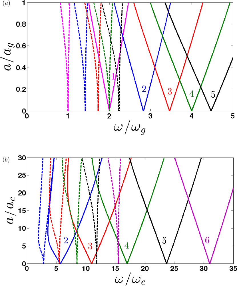
Figure 1: Instability tongues of an inviscid fluid drop due to oscillatory forcing with amplitude $a$ and angular frequency $\omega$. Solid curves bound subharmonic tongues and dashed curves bound harmonic tongues. (a) Tongues corresponding to gravitational instability with spherical wavenumbers $\ell=1$, 2, 3, 4 originate at $\omega/\omega_{g}=2\sqrt{\ell}/n$. (b) Tongues corresponding to capillary instability with spherical wavenumbers $\ell=2$, 3, 4, 5 originate at $\omega/\omega_{c}=2\sqrt{\ell(\ell-1)(\ell+2)}/n$, with $n$ odd (even) for subharmonic (harmonic) tongues.

Figure 2: Same data as in figure 1, but scaled by $\omega_{0}$ and $a_{0}$. The tongues for the gravitational and the capillary cases and for all values of $\ell$ all collapse onto a single set of tongues. Solid curves bound subharmonic tongues and dashed curves bound harmonic tongue.

It is useful to examine (60) and (62) in the two limits of gravity and capillary waves. We first define non-dimensional angular frequencies and oscillation amplitudes which do not depend on $\ell$:

$$\omega_{g}^{2}\equiv\frac{g}{R} \qquad a_{g}\equiv R\omega_{g}^{2}=g$$ (65)

$$\omega_{c}^{2}\equiv\frac{\sigma}{\rho R^{3}} \qquad a_{c}\equiv R\omega_{c}^{2}$$ (66)

so that

$$\omega_{0}^{2} = \omega_{g}^{2}\;\ell+\omega_{c}^{2}\;\ell(\ell-1)(\ell+2)$$ (67)

$$a_{0} = a_{g}+a_{c}(\ell-1)(\ell+2)$$ (68)

The Bond number measuring the relative importance of the two forces can be written as:

$$Bo\equiv\frac{\rho gR^{2}}{\sigma}=\frac{\omega_{g}^{2}}{\omega_{c}^{2}}$$ (69)

In the gravity-dominated regime (large $Bo$), we write (64) as

$$\omega^{2}=\left(\frac{2}{n}\right)^{2}\omega_{g}^{2}\;\left[\ell+\frac{1}{Bo}\ell(\ell-1)(\ell+2)\right]$$ (70)

The stability boundaries for $1/Bo=0$ are given in figure 1(a). The subharmonic and harmonic tongues originate at $\omega/\omega_{g}=2\sqrt{\ell}$ and $\omega/\omega_{g}=\sqrt{\ell}$.

In the capillary-dominated regime (small $Bo$) it is more appropriate to write (64) as

$$\omega^{2}=\left(\frac{2}{n}\right)^{2}\omega_{c}^{2}\left[\ell(\ell-1)(\ell+2)+Bo\;\ell\right]$$ (71)

The stability boundaries for $Bo=0$ are given in figure 1(b) in terms of $\omega/\omega_{c}$ and $a/a_{c}$. These consist of families of tongues, which originate on the $a=0$ axis at $\omega/\omega_{c}=2\sqrt{\ell(\ell-1)(\ell+2)}/n$ for $\ell=2$, 3, 4, 5 and for $n=1$, 2, … within which the drop has one of the spatial forms corresponding to the spherical wavenumber $\ell$ and oscillates like $e^{in\omega t/2}$. The solid curves bound the first subharmonic instability tongues, which orginate on the $a=0$ axis at $\omega/\omega_{c}=2\sqrt{\ell(\ell-1)(\ell+2)}$ for $\ell=2$, 3, 4, 5, within which the drop oscillates like $e^{i\omega t/2}$. The dashed curves bound the first harmonic tongues, originating at $\omega/\omega_{c}=\sqrt{\ell(\ell-1)(\ell+2)}$ describing a response like $e^{i\omega t}$. Tongues for higher $n$ are located at still lower values of $\omega$.

The curves in figure 1 for different $\ell$, $g$, $\sigma/\rho$, $R$ all collapse onto a single set of tongues when they are plotted in terms of $\omega/\omega_{0}$ and $a/a_{0}$. This is shown in figure 2, in which the various tongues correspond to the temporal harmonic index $n$. In order to use figure 2 to determine whether the drop is stable against perturbations with spherical wavenumber $\ell$ when a radial force with amplitude $a$ and angular frequency $\omega$ is applied, the following procedure must be used.

For each $\ell$, formulas (60) and (62) are used to determine the values of $(\omega_{0},a_{0})$, If $(\omega/\omega_{0},a/a_{0})$ is inside one of the instability tongues (usually, but not always, that corresponding to an $\omega/2$ response with $n=1$) then the drop is unstable to perturbations of that $\ell$. The drop is stable if $(\omega/\omega_{0},a/a_{0})$ lies outside the tongues for all $\ell$ and all $n$. This is the procedure described by Benjamin & Ursell (1954) and carried out by Batson et al. (2013) in a cylindrical geometry.

Because $(\omega/\omega_{0},a/a_{0})$ depends on the unknown $\ell$, an experimental or numerical choice of parameters cannot immediately be assigned to a point in figure 2, rendering its interpretation somewhat more obscure. It is perhaps because of this that investigations of the Faraday instability are often presented in dimensional terms. Figures like 1(a) and (b), in which the two axes are non-dimensional quantities defined in terms of known parameters, represent a good compromise between universality and ease of use. This treatment can also be applied to non-spherical geometries in which the unperturbed surface is flat and the depth is finite.

5 Viscous fluids and scaling laws

We now return to the viscous case. For a viscous fluid, it is not possible to reduce the governing equations to a Mathieu equation even with the addition of a damping term (Kumar & Tuckerman, 1994). As described in section 3.2, the governing equations and boundary conditions are reduced to an eigenvalue problem, whose solution gives the critical oscillation amplitude $a$ as an eigenvalue.

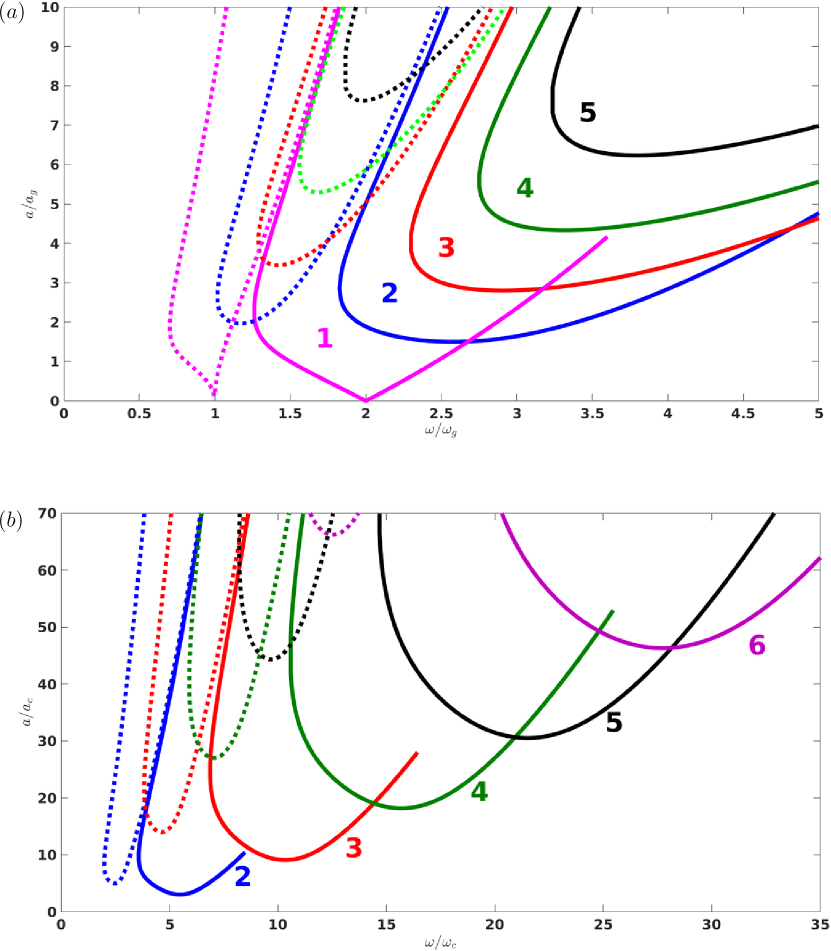
Figure 3: Instability tongues due to oscillatory forcing of amplitude $a$ and angular frequency $\omega$ for a viscous fluid drop. Solid curves bound subharmonic tongues and dashed curves bound harmonic tongues. (a) Tongues corresponding to gravitational instability with viscosity $\nu/\sqrt{gR^{3}}=0.08$. Spherical wavenumbers are $\ell=1$ (magenta), 2 (blue), 3 (red), 4 (green), 5 (black). (b) Tongues correspond to capillary instability with viscosity $\nu/\sqrt{\sigma R/\rho}=0.08$. Spherical wavenumbers are $\ell=2$ (blue), 3 (red), 4 (green), 5 (black), 6 (purple).

Figure 3 displays the regions of instability of a viscous drop using the same conventions as we did for the ideal fluid case, i.e. treating capillary and gravitational instability separately and plotting the stability boundaries in units of $\omega_{c}$, $\omega_{g}$, $a_{c}$, $a_{g}$. Viscosity smoothes the instability tongues and displaces the critical forcing amplitude towards higher values, with a displacement which increases with $\ell$. The viscosity used in figure 3 is $\nu/\sqrt{\sigma R/\rho}=0.08$ and $\nu/\sqrt{gR^{3}}=0.08$ the Ohnesorge number and the inverse square root of the Galileo number for the capillary and the gravitational cases, respectively. This value is chosen to be high enough to show the important qualitative effect of viscosity, but low enough to permit the first few tongues to be shown on a single diagram. It can be seen that the effect of viscosity is greater on tongues with higher $\ell$; this important point will be discussed below. For low enough frequency, i.e. $\omega/\omega_{c}\lesssim 1.2$ in figure 3(a) and $\omega/\omega_{g}\lesssim 4$ in figure 3(b), it can be seen that the instability is harmonic rather than subharmonic, as discussed by Kumar (1996).

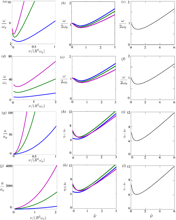
Figure 4: Viscosity dependence of $\omega$ (rows 1 and 2) and $a$ (rows 3 and 4) at threshold. Gravitational (rows 1 and 3) and capillary (rows 2 and 4) Faraday instability shown for $\ell=2$ (blue), 4 (green), and 6 (purple). Leftmost column (a,d,g,j) $\omega$ and $a$ non-dimensionalized in terms of experimentally imposed quantities $\omega_{g}$, $\omega_{c}$, $a_{g}$ and $a_{c}$. Non-dimensionalization of middle column (b,e,h,k) uses (4a) and (4a). It can be seen that $a\sim\nu$ for $\nu$ small. Right column (c,f,i,l) shows analogous quantities for the planar infinite-depth case, calculated using (4b) and (4b); the scaling is seen to be exact in this case.

Figure 4 shows the variation with viscosity of the Faraday threshold, more specifically of the coordinates $(\omega,a)$ of the minimum of the primary subharmonic tongue, for $\ell=2,4,6$ for the capillary and gravitational Faraday instability. The first column shows this dependence using non-dimensional quantities that are independent of $\ell$. (We explained the motivation for such a choice in section 4, namely that $\ell$ is not known a priori in an experiment or full numerical simulation.) The second column shows the non-dimensionalization that best fits the data for all values of $\ell$. The appropriate choice for the non-dimensionalization of viscosity is

$$\tilde{\nu}\equiv\frac{\nu\ell(\ell+1)}{R^{2}\omega_{0}}\qquad\mbox{or}\qquad\tilde{\nu}\equiv\frac{\nu k^{2}}{\omega_{0}}$$ (72a,b)

in the spherical or planar geometries, respectively, based on the wavelength. See Bechhoefer et al. (1995), who studied the influence of viscosity on Faraday waves. The choice of (4) is guided by comparing the viscous and oscillatory terms in (53) and corroborated by the fact that the curves in the second column have only a weak dependence on $\ell$ and on $\tilde{\nu}$. We recall that the ratio of the horizontal (angular) wavelength $2\pi R/\ell$ to the depth (radius) $R$ goes to zero as $\ell$ increases, and the curvature of the sphere is less manifested over a horizontal wavelength. With increasing $\ell$, the curves for the spherical case can be seen to approach the corresponding quantities in the planar infinite-depth case, shown in the third column, despite the fact that we are far from the large $\ell$ limit.

Figures 4(a)-(f) show that the frequency $\omega$ which favours waves (corresponding to the bottom of the tongue) is a non-monotonic function of $\nu$, for which an explanation is proposed by Kumar & Tuckerman (1994). At lower viscosities, the flow is assumed to be irrotational, as in (56), and equation (60) is modified merely by subtracting a term proportional to $\nu^{2}$. This leads to a decrease in the critical $\omega$ from $2\omega_{0}$. At higher viscosities, it is assumed that the response time $4\pi/\omega$ approaches the viscous time scale, here $O(\ell(\ell+1)R^{2}/\nu)$, leading to an increase in $\omega$ with $\nu$ when the other parameters are fixed. Experimental values for $\tilde{nu}$ are, however, rarely greater than one.

Concerning the oscillation amplitude $a$, we find that the appropriate choice for non-dimensionalization is

$$\tilde{a}\equiv\frac{a\ell}{R\omega_{0}^{2}}\qquad\mbox{or}\qquad\tilde{a}\equiv\frac{ak}{\omega_{0}^{2}}$$ (73a,b)

This non-dimensionalization causes all six curves of figure 4(g) and (j) to collapse. For small viscosities, $\tilde{a}$ increases linearly with $\tilde{\nu}$; see Bechhoefer et al. (1995). For this reason we plot

$$\frac{\tilde{a}}{\tilde{\nu}}=\frac{a\ell}{R\omega_{0}^{2}}\left(\frac{\nu\ell(\ell+1)}{R^{2}\omega_{0}}\right)^{-1}=\frac{aR}{\nu\omega_{0}(\ell+1)}\qquad\mbox{or}\qquad\frac{\tilde{a}}{\tilde{\nu}}=\frac{a}{\nu\omega_{0}k}$$ (74a,b)

in figures 4(h,i,k,l). The form of this curve for higher viscosities shows that $\tilde{a}$ contains terms of higher order in $\tilde{\nu}$, as demonstrated by Vega et al. (2001).

The viscosity dependence of $\omega$ and $a$, once they are non-dimensionalized, are practically identical for the capillary and gravitational cases. The difference between these, as well as the dependence on $\ell$, is taken into account exclusively via $\omega_{0}(\ell)$, just as it is for the inviscid problem.

6 Eigenmodes

Thus far, we have not discussed the spatial form of the eigenmodes on the interface, beyond stating that they are spherical harmonics. Visualizations of the spherical harmonics, while common, are inadequate or incomplete for depicting the behaviour of the interface in this problem for a number of reasons. First, as stated in the introduction, the linear stability problem is degenerate: the $2\ell+1$ spherical harmonics which share the same $\ell$ all have the same linear growth rates and threshold. Second, for $\ell\geq 4$, the patterns actually realized in experiments or numerical simulations, which are determined by the nonlinear terms, are not individual spherical harmonics, but particular combinations of them. Finally, in a Floquet problem, the motion of the interface is time dependent.

Figure 5 shows the spherical harmonics for $\ell=4$. Spherical harmonics can be classified as zonal ($m=0$, independent of $\phi$, nodal lines which are circles of constant latitude), sectoral ($m=\pm\ell$, independent of $\theta$, nodal lines which are circles of constant longitude), or tesseral ($m\neq 0,\pm\ell$, checkered). Figure 6 depicts the pattern that is realized in numerical simulations for $\ell=4$. The pattern oscillates between a cube and an octahedron and is a combination of $Y_{4}^{0}$ and $Y_{4}^{4}$. This pattern is the result of nonlinear selection; at the linear level, many other patterns could be realized. Our companion paper is devoted to a comprehensive description of the motion of the interface and of the velocity field for $\ell$ between 1 and 6.

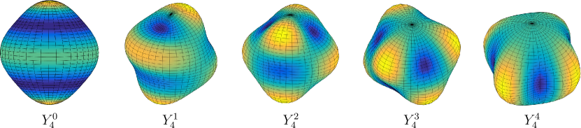
Figure 5: Spherical harmonics for $\ell=4$.

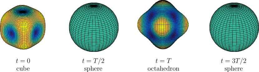
Figure 6: Subharmonic $\ell=4$ standing wave pattern oscillates in time between cubic and octahedral shapes.

7 Discussion

We have considered a configuration similar to the classic problem of freely oscillating liquid drops, that of a viscous drop under the influence of a time-periodic radial bulk force and of surface tension. Here, we have carried out a linear stability analysis, while in a companion paper Ebo-Adou et al. (2019), we describe the results of a full numerical simulation. We believe both of these investigations to be the first of their kind.

Our investigation relies on a variety of mathematical and computational tools. We have solved the linear stability problem by adapting to spherical coordinates the Floquet method of Kumar & Tuckerman (1994). The solution method uses a spherical harmonic decomposition in the angular directions and a Floquet decomposition in time to reduce the problem to a series of radial equations, whose solutions are monomials and spherical Bessel functions. We find that the equations for the inviscid case reduce exactly to the Mathieu equation, as they do for the planar case Benjamin & Ursell (1954), with merely a reassignment of the parameter definitions. In contrast, for the viscous case, there are additional terms specific to the spherical geometry.

The forcing parameters for which the spherical drop is unstable are organized into tongues. The effect of viscosity is to raise, to smooth, and to distort the instability tongues, both with increasing $\nu$ and also with increasing spherical wavenumber $\ell$. Our computations have demonstrated the appropriate scaling for the critical oscillation frequency and amplitude with viscosity, substantially reducing the large parameter space of the problem.

The nonlinear problem is fully three-dimensional and must be treated numerically. In our companion paper (Ebo-Adou et al., 2019), we will describe and analyse the patterns corresponding to various values of $\ell$ that we have computed by forcing a viscous drop at appropriate frequencies.

Acknowledgements

We thank Stéphan Fauve and David Quéré for helpful discussions.

Appendix A Appendix

A.1 Boundary conditions for the two-fluid case

We describe here the modifications necessary in order to take into account the fluid medium surrounding the drop of radius $R$, occupying either a finite sphere of radius $R_{\rm out}$ or an infinite domain. The inner and outer density, dynamic viscosity and poloidal fields are denoted by $\rho_{j}$, $\eta_{j}$, and $f^{(j)}$ for $j=1,2$. $\Delta\Psi\equiv\left[\Psi^{(2)}-\Psi^{(1)}\right]_{r=R}$ denotes the jump of any quantity $\Psi$ across the interface and applies to all quantities to its right within a term. For each spherical harmonic wavenumber $\ell$ and each Floquet mode $n$, the poloidal fields $f_{n}^{(j)}$ given in (48) are as follows:

$$f_{n}^{(1)}(r) =A_{n}^{(1)}r^{\ell+1}+B_{n}^{(1)}r^{\frac{1}{2}}J_{\ell+\frac{1}{2}}(iq_{n}^{(1)}r)$$ (75a)

$$f_{n}^{(2)}(r) =A_{n}^{(2)}r^{\ell+1}+B_{n}^{(2)}r^{\frac{1}{2}}J_{\ell+\frac{1}{2}}(iq_{n}^{(2)}r)+C_{n}^{(2)}r^{-\ell}+D_{n}^{(2)}r^{\frac{1}{2}}J_{-\left(\ell+\frac{1}{2}\right)}(iq_{n}^{(2)}r)$$ (75b)

where

$$q_{n}^{(j)}\equiv\left[\frac{\mu+i(n\omega+\alpha)}{\nu_{j}}\right]^{1/2}$$ (76)

The introduction of four more constants requires four additional conditions. Two of these are provided by the exterior boundary conditions. The relations

$$0 =u_{r}=\frac{\ell(\ell+1)}{r^{2}}f$$ (77a)

$$0 =\nabla_{H}\cdot\mathbf{u}_{H}=\frac{1}{r^{2}}\frac{\partial}{\partial r}r^{2}u_{r}=\frac{1}{r^{2}}\frac{\partial}{\partial r}\ell(\ell+1)$$ (77b)

imply that both $f^{(2)}_{n}$ and its radial derivative must vanish at $R_{\rm out}$:

$$0=f^{(2)}_{n}(R_{\rm out})=f^{(2)\prime}_{n}(R_{\rm out})$$ (78)

If the exterior is infinite, then $A_{n}^{(2)}=B_{n}^{(2)}=0$; otherwise equations (78) couple the six constants. Continuity of the velocity at $r=R$, together with (77) provides the remaining two additional conditions:

$$0=\Delta f=\Delta f^{\prime}$$ (79)

The kinematic condition (50) remains unchanged:

$$(\mu+i(n\omega+\alpha)) \zeta_{n}=\frac{\ell(\ell+1)}{R^{2}}f_{n}|_{r=R}$$ (80)

since $f$ is continuous across the interface, while the tangential stress condition (51) becomes

$$0=\Delta\left[\eta\left(\frac{\partial^{2}}{\partial r^{2}}-\frac{2}{r}\frac{\partial}{\partial r}+\frac{\ell(\ell+1)}{r^{2}}\right)f_{n}\right]$$ (81)

The pressure jump condition (53) becomes

$$0=\Delta\left[\rho(\mu+i(n\omega+\alpha))\frac{\partial}{\partial r}\right. \left.-\eta\left(\frac{\partial^{3}}{\partial r^{3}}+\frac{2}{r}\frac{\partial^{2}}{\partial r^{2}}-\ell(\ell+1)\left(\frac{3}{r^{2}}\frac{\partial}{\partial r}-\frac{4}{r^{3}}\right)\right)f_{n}\right.$$

$$+\left.\left(\rho g+\sigma\frac{(\ell-1)(\ell+2)}{R^{2}}\right)\zeta_{n}-\rho\frac{a}{2}(\zeta_{n+1}+\zeta_{n-1})\right]$$ (82)

where $\rho$, $\eta$, $\partial^{2}f/\partial r^{2}$ and $\partial^{3}f/\partial r^{3}$ are all discontinuous across the interface.

A.2 Differentiation relations

We express the governing equations in terms of the constants $A_{n}$, $B_{n}$, $C_{n}$, $D_{n}$ via

$$f_{n}(r) =A_{n}r^{\ell+1}+B_{n}r^{\frac{1}{2}}J_{+}+C_{n}r^{-\ell}+D_{n}r^{\frac{1}{2}}J_{-}$$ (83a)

$$\frac{\partial}{\partial r}f_{n}(r) =A_{n}(l+1)r^{\ell}+B_{n}\left(\frac{1}{2}r^{-\frac{1}{2}}J_{+}+iq_{n}r^{\frac{1}{2}}J_{+}^{\prime}\right)$$

$$-C_{n}\ell r^{-\ell-1}+D_{n}\left(\frac{1}{2}r^{-\frac{1}{2}}J_{-}+iq_{n}r^{\frac{1}{2}}J_{-}^{\prime}\right)$$ (83b)

$$\frac{\partial^{2}}{\partial r^{2}}f_{n}(r) =A_{n}\ell(\ell+1)r^{\ell-1}+B_{n}\left(-\frac{1}{4}r^{-\frac{3}{2}}J_{+}+iq_{n}r^{-\frac{1}{2}}J_{+}^{\prime}-q_{n}^{2}r^{\frac{1}{2}}J_{+}^{\prime\prime}\right)$$

$$+C_{n}\ell(\ell+1)r^{-\ell-2}+D_{n}\left(-\frac{1}{4}r^{-\frac{3}{2}}J_{-}+iq_{n}r^{-\frac{1}{2}}J_{-}^{\prime}-q_{n}^{2}r^{\frac{1}{2}}J_{-}^{\prime\prime}\right)$$ (83c)

$$\frac{\partial^{3}}{\partial r^{3}}f_{n}(r) =A_{n}(\ell+1)\ell(\ell-1)r^{\ell-2}+B_{n}\left(\frac{3}{8}r^{-\frac{5}{2}}J_{+}-\frac{3}{4}iq_{n}r^{-\frac{3}{2}}J_{+}^{\prime}-\frac{3}{2}q_{n}^{2}r^{-\frac{1}{2}}J_{+}^{\prime\prime}-iq_{n}^{3}r^{\frac{1}{2}}J_{+}^{\prime\prime\prime}\right)$$

$$-C_{n}\ell(\ell+1)(\ell+2)r^{-\ell-3}+D_{n}\left(\frac{3}{8}r^{-\frac{5}{2}}J_{-}-\frac{3}{4}iq_{n}r^{-\frac{3}{2}}J_{-}^{\prime}-\frac{3}{2}q_{n}^{2}r^{-\frac{1}{2}}J_{-}^{\prime\prime}-iq_{n}^{3}r^{\frac{1}{2}}J_{-}^{\prime\prime\prime}\right)$$ (83d)

where $J_{+}$ and $J_{-}$ denote $J_{\ell+\frac{1}{2}}$ and $J_{-\left(\ell+\frac{1}{2}\right)}$, respectively, to be evaluated at $iq_{n}^{(j)}R$. To evaluate the derivatives of the Bessel functions, we use the recurrence relations:

$$J^{\prime}_{\nu}(z) =\frac{1}{2}\left(J_{\nu-1}(z)-J_{\nu+1}(z)\right)$$ (84a)

$$J^{\prime\prime}_{\nu}(z) =\frac{1}{4}\left(J_{\nu-2}(z)-2J_{\nu}(z)+J_{\nu+2}(z)\right)$$ (84b)

$$J^{\prime\prime\prime}_{\nu}(z) =\frac{1}{8}\left(J_{\nu-3}(z)-3J_{\nu-1}(z)+3J_{\nu+1}(z)-J_{\nu+3}(z)\right)$$ (84c)

For the two-fluid case, we express the seven conditions (78), (79), (80), (81) and (82) in terms of the constants $A^{(j)}_{n}$, $B^{(j)}_{n}$, $C^{(j)}_{n}$, $D^{(j)}_{n}$, and $\zeta_{n}$. For the single-fluid case, we express the three conditions (50), (51), (53) in terms of $A_{n}$, $B_{n}$, and $\zeta_{n}$. Omitting the pressure jump condition leads to a $6\times 6$ (finite outer sphere), $4\times 4$ (infinite outer sphere), or $2\times 2$ (single-fluid) system which can be inverted to obtain values for all of the constants as multiples of $\zeta_{n}$. The pressure jump condition is then a Floquet problem in $\{\zeta_{n}\}$, solved as described in section 3.2.

References

- Abramowitz & Stegun (1965) Abramowitz, M. & Stegun, I.A. 1965 Handbook of Mathematical Functions. Dover Publications.
- Batson et al. (2013) Batson, W., Zoueshtiagh, F. & Narayanan, R. 2013 The Faraday threshold in small cylinders and the sidewall non-ideality. J. Fluid Mech. 729, 496–523.
- Bechhoefer et al. (1995) Bechhoefer, J., Ego, V., Manneville, S. & Johnson, B. 1995 An experimental study of the onset of parametrically pumped surface waves in viscous fluids. J. Fluid Mech. 288, 325–350.
- Benjamin & Ursell (1954) Benjamin, T. B. & Ursell, F. 1954 The stability of the plane free surface of a liquid in vertical periodic motion. Proc. R. Soc. Lond. 225, 505–515.
- Brunet & Snoeijer (2011) Brunet, P. & Snoeijer, J. H. 2011 Star-drops formed by periodic excitation and on an air cushion–a short review. Eur. Phys. J. Special Topics 192 (1), 207–226.
- Chandrasekhar (1961) Chandrasekhar, S. 1961 Hydrodynamic and Hydromagnetic Stability. Oxford University Press.
- Cummings & Blackburn (1991) Cummings, D. L. & Blackburn, D. A. 1991 Oscillations of magnetically levitated aspherical droplets. J. Fluid Mech. 224, 395–416.
- Ebo-Adou et al. (2019) Ebo-Adou, A., Tuckerman, L.S., Shin, S., Chergui, J. & Juric, D. 2019 Faraday instability on a sphere: Numerical simulation. J. Fluid Mech. 870, 433–459.
- Falcón et al. (2009) Falcón, C., Falcon, E., Bortolozzo, U. & Fauve, S. 2009 Capillary wave turbulence on a spherical fluid surface in low gravity. Europhys. Lett. 86, 14002.
- Futterer et al. (2013) Futterer, B., Krebs, A., Plesa, A. C., Zaussinger, F., Hollerbach, R., Breuer, D. & Egbers, C. 2013 Sheet-like and plume-like thermal flow in a spherical convection experiment performed under microgravity. J. Fluid Mech. 735, 647–683.
- Kelvin (1863) Kelvin, Sir Lord 1863 Elastic spheroidal shells and spheroids of incompressible liquid. Philos. Trans. R. Soc. London 153, 583.
- Kumar (1996) Kumar, K. 1996 Linear theory of Faraday instability in viscous fluids. Proc. R. Soc. Lond. 452, 1113–1126.
- Kumar & Tuckerman (1994) Kumar, K. & Tuckerman, L. S. 1994 Parametric instability of the interface between two fluids. J. Fluid Mech. 279, 49–68.
- Lamb (1932) Lamb, H. 1932 Hydrodynamics. Cambridge University Press.
- Marston (1980) Marston, P. L. 1980 Shape oscillation and static deformation of drops and bubbles driven by modulated radiation stresses-—theory. J. Acoust. Soc. Am. 67 (1), 15–26.
- Miller & Scriven (1968) Miller, C. A. & Scriven, L. E. 1968 The oscillations of a fluid droplet immersed in another fluid. J. Fluid Mech. 32, 417–435.
- Prosperetti (1980) Prosperetti, A. 1980 Normal-mode analysis for the oscillations of a viscous liquid drop in an immiscible liquid. J. Mec. 19, 149–182.
- Rayleigh (1879) Rayleigh, Lord 1879 On the capillary phenomena of jets. Proc. R. Soc. Lond. 29, 71–97.
- Reid (1960) Reid, W. H. 1960 The oscillations of a viscous liquid drop. Q. Appl. Math. 18, 86–89.
- Shen et al. (2010) Shen, C. L., Xie, W. J. & Wei, B 2010 Parametrically excited sectorial oscillation of liquid drops floating in ultrasound. Phys. Rev. E 81 (4), 046305.
- Trinh & Wang (1982) Trinh, E. & Wang, T. G. 1982 Large-amplitude free and driven drop-shape oscillations: experimental observations. J. Fluid Mech. 122, 315–338.
- Trinh et al. (1982) Trinh, E, Zwern, A & Wang, T. G. 1982 An experimental study of small-amplitude drop oscillations in immiscible liquid systems. J. Fluid Mech. 115, 453–474.
- Tsamopoulos & Brown (1983) Tsamopoulos, J. A. & Brown, R. A. 1983 Nonlinear oscillations of inviscid drops and bubbles. J. Fluid Mech. 127, 514–537.
- Vega et al. (2001) Vega, J. M., Knobloch, E. & Martel, C. 2001 Nearly inviscid Faraday waves in annular containers of moderately large aspect ratio. Physica D 154, 313–336.
- Wang et al. (1996) Wang, T. G., Anilkumar, A. V. & Lee, C. P. 1996 Oscillations of liquid drops: results from USML-1 experiments in space. J. Fluid Mech. 308, 1–14.