Reconstruction-Aware Imaging System Ranking by use of a Sparsity-Driven Numerical Observer Enabled by Variational Bayesian Inference

Abstract

It is widely accepted that optimization of imaging system performance should be guided by task-based measures of image quality (IQ). It has been advocated that imaging hardware or data-acquisition designs should be optimized by use of an ideal observer (IO) that exploits full statistical knowledge of the measurement noise and class of objects to be imaged, without consideration of the reconstruction method. In practice, accurate and tractable models of the complete object statistics are often difficult to determine. Moreover, in imaging systems that employ compressive sensing concepts, imaging hardware and sparse image reconstruction are innately coupled technologies. In this work, a sparsity-driven observer (SDO) that can be employed to optimize hardware by use of a stochastic object model describing object sparsity is described and investigated. The SDO and sparse reconstruction method can therefore be “matched” in the sense that they both utilize the same statistical information regarding the class of objects to be imaged. To efficiently compute the SDO test statistic, computational tools developed recently for variational Bayesian inference with sparse linear models are adopted. The use of the SDO to rank data-acquisition designs in a stylized example as motivated by magnetic resonance imaging (MRI) is demonstrated. This study reveals that the SDO can produce rankings that are consistent with visual assessments of the reconstructed images but different from those produced by use of the traditionally employed Hotelling observer (HO).

I Introduction

The development of methodologies for optimizing imaging system performance remains an important and actively investigated topic. It is widely accepted that optimization of imaging system performance should be guided by task-based measures of image quality (IQ) [1, 2, 3, 4, 5, 6, 7]. Signal detection tasks [8, 9], such as tumor detection, are ubiquitous and relevant to a wide range of medical imaging modalities [10]. An upper performance bound for a binary detection task is achieved by the Bayesian ideal observer (IO) [1, 8, 11], which is a numerical observer that employs complete knowledge of the object and the noise statistics. Henceforth, any reference to IOs refers to Bayesian IOs.

It has been widely advocated to use IO performance, evaluated by use of an ensemble of experimental or simulated measurement data, as a figure-of-merit (FOM) to guide optimization of imaging hardware and data-acquisition parameters for signal-detection tasks. A rationale for this is that the IO detection performance can be interpreted as a measure of the ability of the imaging system to record a signal optimally distinguished from the background structures and measurement noise. The IO has also been employed to assess the efficiency of human observers on signal detection tasks[12].

The IO performs the likelihood-ratio test for a classification task and thus the test statistic is a ratio of posterior probability distributions under competing hypotheses. This alone is a substantial impediment to using the true IO because it requires knowledge of the full probability density function (PDF) that describes the ensemble of objects to be imaged. Henceforth, this PDF will be referred to as a stochastic object model (SOM). While SOMs have been proposed for applications that include nuclear medicine imaging[13, 14] and breast imaging[15], accurate and tractable models of object statistics generally are not available for most imaging applications. Moreover, even if a suitable SOM is available, computation of the likelihood ratio, in general, is not analytically tractable and remains computationally burdensome.

Markov chain Monte Carlo (MCMC) techniques [16] have been proposed to compute IO performance for a specific class of object model such as the lumpy or clustered lumpy object models or parameterized phantoms[17]. In principle, the MCMC methods can provide unbiased results; however, their application is limited by long computation time, sometimes extending to weeks. Another disadvantage is that considerable expertise is required to run the MCMC simulations properly. We are unaware of any convergence diagnostics that are simple to use or even widely accepted. In practice, due to these complications, application of MCMC methods has been limited to relatively simple stochastic object models and relatively small image sizes.

In recent years, motivated by the theory of compressive sensing, there has been a paradigm shift in the way that images are formed in computed imaging systems. Modern sparse reconstruction methods exploit the fact that many objects of interest can typically be described by use of sparse representations. Sparse reconstruction methods have proven to be highly effective at reconstructing images from under-sampled measurement data in a wide range of medical imaging systems including magnetic resonance imaging (MRI) [18, 19, 20] and X-ray computed tomography (CT)[21, 22, 23].

While a vast amount of research has been conducted on the development of sparse reconstruction methods, very little research has addressed the problem of how to optimize data-acquisition designs for specific diagnostic tasks when sparse reconstruction methods are employed. The minimum amount and quality of measurement data required for estimation of an image of prescribed accuracy or utility is affected by the sparsity properties of the object and the specification of the sparse reconstruction method [7]. Intuitively, this is to be expected because different sparse reconstruction methods exploit different a priori information about the object. The sparsity-promoting regularization penalties employed by a reconstruction method can be associated with SOMs (i.e., object priors) within a Bayesian framework. However, this seems inconsistent with the conventional notion [1, 3] that suggests that hardware and data-acquisition designs should be optimized by use of an IO and the measurement data, independent of the choice of image reconstruction method. A potential explanation for this inconsistency is that, in modern imaging systems that employ compressive sensing concepts, imaging hardware and sparse image reconstruction are innately coupled technologies.

In this work, a new numerical observer is developed for signal-known-exactly (SKE) detection tasks that can be employed to optimize data-acquisition designs for computed imaging systems when sparse reconstruction methods are employed. The new numerical observer is referred to as a sparsity-driven observer (SDO). Similar to other approximated IOs, the SDO acts on the measurement data and employs the likelihood ratio as test statistics. The key difference is that where traditional IOs (and approximations thereof) are predicated upon comprehensive statistical knowledge of the objects imaged, the SDO assumes an SOM that describes only the sparsity properties of the class of objects. In this way, the SDO and sparse reconstruction method will be “matched” in the sense that they both utilize the same statistical information regarding the class of objects to be imaged. This information is already known to be useful for sparse reconstruction methods. As such, the use of the SDO will permit task-specific optimization of data-acquisition designs with consideration of the (non-linear) sparse reconstruction method to-be-employed.

The remainder of the article is organized as follows. In Section II, necessary background from signal detection theory and sparse image reconstruction is provided. The SDO for the case of i.i.d. Gaussian measurement noise is defined in Section III and a semi-analytic procedure for computing it based on variational Bayesian inference for sparse linear models is presented. The validity of the variational approximation employed to compute the SDO test statistic is investigated in Section IV. In Section V, the use of the SDO to rank-order data-acquisition designs in a stylized example motivated by magnetic resonance imaging (MRI) is demonstrated. Finally, the article concludes with a discussion of the SDO in Section VI.

II Background

II-A The Likelihood Ratio Calculation for Binary Classification Tasks

Consider a discrete-to-discrete linear imaging model (see sec 7.4 in [1])

$$\mathbf{g}=\mathbf{H}\mathbf{f}+\mathbf{n},$$ (1)

which we will consider to be an accurate approximation of the true continuous-to-discrete tomographic imaging model. Here, $\mathbf{H}:\mathbb{E}^{N}\rightarrow\mathbb{E}^{M}$ denotes the system matrix. The vectors $\mathbf{g}\in\mathbb{E}^{M}$ and $\mathbf{n}\in\mathbb{E}^{M}$ denote the discrete measurement data and random noise, respectively. In this preliminary study, $\mathbf{n}$ corresponds to a random vector whose components are independent and identically distributed (i.i.d.) Gaussian random variables with zero mean and variance $\sigma^{2}$. The vector $\mathbf{f}\in\mathbb{E}^{N}$ represents a finite-dimensional approximation of the measured object’s property distribution.

A signal-known-exactly (SKE) and background-known-statistically (BKS) binary detection task is considered[1]. The object vector $\mathbf{f}$ will be expressed as $\mathbf{f}=\mathbf{f}_{b}+\mathbf{f}_{s}$, where $\mathbf{f}_{s}$ denotes the known signal and $\mathbf{f}_{b}$ denotes the random background. The binary signal-detection task requires deciding between the signal absent and signal present hypotheses, denoted as $\mathcal{H}_{0}$ and $\mathcal{H}_{1}$:

$$\mathcal{H}_{0}:\,\mathbf{g}=\mathbf{H}\mathbf{f}_{b}+\mathbf{n};\,\,\mathcal{H}_{1}:\,\mathbf{g}=\mathbf{H}(\mathbf{f}_{b}+\mathbf{f}_{s})+\mathbf{n}.$$ (2)

Because we have not introduced notation to differentiate random from non-random vectors, it should be emphasized that, in the SKE-BKS detection task, $\mathbf{f}_{b}$, $\mathbf{n}$, and $\mathbf{g}$ are random vectors, while $\mathbf{f}_{s}$ is non-random.

To make a decision, the IO employs a test statistic corresponding to the likelihood ratio:

$$\Lambda(\mathbf{g})=\frac{P(\mathbf{g}|\mathcal{H}_{1})}{P(\mathbf{g}|\mathcal{H}_{0})},$$ (3)

where $P(\mathbf{g}|\mathcal{H}_{i})$ denotes the conditional PDF of the data vector under the hypothesis $\mathcal{H}_{i}$ ($i=0,1$). It is well-known that the IO decision strategy is optimal in the sense that it yields the best possible receiver operating characteristics (ROC) curve[24, 4, 3].

For a SKE/BKS detection task, the likelihood ratio test statistic can be calculated as (see [16] and Sec 13.2 in [1])

$$\Lambda(\mathbf{g})=\int\mathop{}\!\mathrm{d}\mathbf{f}_{b}\,\Lambda_{BKE}(\mathbf{g}|\mathbf{f}_{b})P(\mathbf{f}_{b}|\mathbf{g},\mathcal{H}_{0}),$$ (4)

where $\Lambda_{BKE}(\mathbf{g}|\mathbf{f}_{b})$ is the likelihood ratio for the background-known-exactly (BKE) case, where only the noise vector $\mathbf{n}$ in Eqs. (2) is random, and $P(\mathbf{f}_{b}|\mathbf{g},\mathcal{H}_{0})$ is the posterior PDF that describes $\mathbf{f}_{b}$ under hypothesis $\mathcal{H}_{0}$. Note that the posterior PDF that appears in Eq. (4) can be expressed as

$$P(\mathbf{f}_{b}|\mathbf{g},\mathcal{H}_{0})=\frac{P(\mathbf{f}_{b})P(\mathbf{g}|\mathbf{f}_{b},\mathcal{H}_{0})}{P(\mathbf{g}|\mathcal{H}_{0})}=\frac{P(\mathbf{f}_{b})P(\mathbf{g}|\mathbf{f}_{b},\mathcal{H}_{0})}{\int\mathop{}\!\mathrm{d}\mathbf{f}_{b}P(\mathbf{f}_{b})P(\mathbf{g}|\mathbf{f}_{b},\mathcal{H}_{0})},$$ (5)

where $P(\mathbf{f}_{b})$ denotes the stochastic object model and $P(\mathbf{g}|\mathbf{f}_{b},\mathcal{H}_{0})$ describes the measurement noise under the signal absent hypothesis.

II-B Challenges in Computing the Likelihood Ratio Test Statistic

Except for special cases, a closed form solution for the likelihood ratio test statistic given by Eq. (4) is generally unavailable. A key challenge is determination of the posterior distribution $P(\mathbf{f}_{b}|\mathbf{g},\mathcal{H}_{0})$. To analytically compute this posterior distribution via Eq. (5), closed form expressions for the stochastic object model $P(\mathbf{f}_{b})$ and measurement noise $P(\mathbf{g}|\mathbf{f}_{b},\mathcal{H}_{0})$ must be available. While simple forms for $P(\mathbf{g}|\mathbf{f}_{b},\mathcal{H}_{0})$ may be available – such as with the Gaussian measurement noise model assumed later in this work – simple forms for $P(\mathbf{f}_{b})$ are rarely available. Additionally, the high-dimensional integrals present in Eqs. (4) and (5) may be difficult to compute. When analytical formula are not available for the posterior distribution, sampling methods such as the MCMC method can be employed[16]. However, this method can be computationally intensive and can require expertise to run properly as noted in the introduction.

II-C Maximum a Posteriori (MAP) Estimation Using Sparsity-Promoting Priors

Over the last decade, sparsity has emerged as a widely employed concept in signal processing and image reconstruction[25, 18, 23, 22]. A vector $\mathbf{f}$ is said to be sparse if most of its components are equal to zero. Medical images are, in general, not strictly sparse, but often can be accurately approximated as such in an appropriate transform domain. Expansion coefficients that represent an image in linear transform spaces typically have super-Gaussian distributions (peaked, heavy-tailed) [26].

Sparse reconstruction algorithms employ a simple and well-known statistical model to describe object sparseness. Let $\mathbf{B}\in\mathbb{E}^{N}\rightarrow\mathbb{R}^{Q}$ be a sparsifying transform that maps an object vector $\mathbf{f}\in\mathbb{E}^{N}$ into a transform space as

$$\mathbf{w}=\mathbf{B}\mathbf{f}\in\mathbb{R}^{Q},$$ (6)

where $\mathbf{w}$ is the transformed vector that is designed to be approximately sparse. The dimension $Q$ of the transformed space depends on the sparsifying matrix chosen. Commonly employed choices for $\mathbf{B}$ in the image processing literature include wavelet transforms and discrete first derivatives. The statistical properties of the object that are related to sparsity can be described by an i.i.d. Laplacian distribution[26]:

$$P(\mathbf{f})=\frac{\tau}{2}\prod_{i=1}^{Q}\exp(-\tau|w_{i}|).$$ (7)

Here, $w_{i}$ denotes the $i$-th component of $\mathbf{w}$ and $\tau\geq 0$ is a scale parameter of the Laplacian distribution. The value of $\tau$ determines how peaked about the origin the distribution is, which, in effect, reflects the sparsity of $\mathbf{w}$. For a given ensemble of objects, this parameter can be empirically determined as described in Appendix B. For a suitable choice of $\mathbf{B}$, Eq. (7) will represent a sparse statistical prior.

A sparse statistical prior can be utilized to regularize the image reconstruction problem when maximum a posteriori (MAP) estimation is employed. A MAP estimate of $\mathbf{f}$ is defined as

$$\mathbf{\hat{f}}=\arg\underset{\mathbf{f}}{\max}\,P(\mathbf{f}|\mathbf{g})=-\arg\underset{\mathbf{f}}{\min}\,\log\left[P(\mathbf{g}|\mathbf{f})P(\mathbf{f})\right].$$ (8)

For the special case of i.i.d. Gaussian noise considered below, the likelihood function $P(\mathbf{g}|\mathbf{f})$ is given by

$$P(\mathbf{g}|\mathbf{f}) =\mathcal{N}(\mathbf{g}|\mathbf{H}\mathbf{f},\sigma^{2}\mathbf{I})$$

$$=(2\pi\sigma^{2})^{-M/2}\exp\left(-{||\mathbf{g}-\mathbf{H}\mathbf{f}||^{2}}/{2\sigma^{2}}\right),$$ (9)

where $\sigma^{2}$ denotes the noise variance that is assumed to be object-independent and $\mathbf{I}$ is the $M\times M$ identity matrix. Generalization to a more complex noise model is discussed in Sec. VI. Based on Eqs. (7) and (II-C), the MAP estimate can be computed as

$$\mathbf{\hat{f}}=\arg\underset{\mathbf{f}}{\min}\,\left({||\mathbf{g}-\mathbf{H}\mathbf{f}||^{2}}+2\sigma^{2}\tau\sum_{i=1}^{Q}|w_{i}|\right).$$ (10)

Equation (10) describes a penalized least squares (PLS) estimate of $\mathbf{f}$ that employs an $l_{1}$-norm-based penalty term. This demonstrates the connection between sparse object priors of the form given in Eq. (7) and commonly employed sparse image reconstruction methods.

III Computation of the Sparsity-Driven Observer Test Statistic

Below, the test statistic for the SDO is defined for the case of independent identically distributed (i.i.d.) Gaussian measurement noise. A semi-analytic procedure for computing it based on variational Bayesian inference for sparse linear models is presented subsequently.

III-A Definition of the SDO Test Statistic

Formally, the SDO test statistic is defined by Eq. (4) when the stochastic object model $P(\mathbf{f}_{b})$ that appears in Eq. (5) is specified by a sparse prior of the form given in Eq. (7). In this way, the SDO and sparse reconstruction method described by Eq. (10) will be matched in the sense that they both assume the same statistical information about the class of objects to be imaged.

In this work, we will assume that the components of the noise vector $\mathbf{n}$ are i.i.d. Gaussian random variables having zero mean and variance $\sigma^{2}$. Thus, $\Lambda_{BKE}(\mathbf{g}|\mathbf{f}_{b})$ is given by

$$\Lambda_{BKE}(\mathbf{g}|\mathbf{f}_{b})=\frac{\mathcal{N}(\mathbf{g}|\mathbf{H}(\mathbf{f}_{b}+\mathbf{f}_{s}),\sigma^{2}\mathbf{I})}{\mathcal{N}(\mathbf{g}|\mathbf{H}\mathbf{f}_{b},\sigma^{2}\mathbf{I})}$$

$$=\exp\left[({2\mathbf{g}^{\dagger}\mathbf{H}\mathbf{f}_{s}-\|\mathbf{H}\mathbf{f}_{b}+\mathbf{H}\mathbf{f}_{s}\|^{2}+\|\mathbf{H}\mathbf{f}_{b}\|^{2}})/{2\sigma^{2}}\right],$$ (11)

where $\dagger$ denotes the adjoint.

In order to compute the SDO test statistic according to Eq. (4), the posterior distribution $P(\mathbf{f}_{b}|\mathbf{g},\mathcal{H}_{0})$ needs to be determined for the case where the sparse prior in Eq. (7) and noise model in Eq. (II-C) are assumed. To accomplish this, methods for variational Bayesian inference are employed as described next.

III-B Estimation of $P(\mathbf{f}_{b}|\mathbf{g},\mathcal{H}_{0})$ by use of a Variational Approximation

To circumvent the aforementioned challenges associated with determining $P(\mathbf{f}_{b}|\mathbf{g},\mathcal{H}_{0})$, computational tools developed for variational Bayesian inference with large-scale sparse linear models were employed[27, 28]. Variational inference methods employ an analytical approximation to the posterior probability distribution, and represent alternatives to computationally cumbersome MCMC methods for inference over complicated distributions that are difficult to evaluate or sample. Whereas the MCMC methods provide a numerical approximation to the exact posterior by use of a set of samples, variational Bayesian methods provide a locally optimal, exact analytical solution to an approximation of the posterior distribution[29, 30, 31]. Moreover, compared with the MCMC methods, variational methods have better scalability as the size of the problem increases [16] and can potentially reduce computation times by several orders of magnitude.

By use of the sparse prior in Eq. (7) and likelihood function in Eq. (II-C), the posterior distribution can be expressed as

$$P(\mathbf{f}_{b}|\mathbf{g},\mathcal{H}_{0})_{P(\mathbf{f}_{b})}=Z^{-1}\mathcal{N}(\mathbf{g}|\mathbf{H}\mathbf{f}_{b},\sigma^{2}\mathbf{I})\prod_{i=1}^{Q}\exp(-\tau|w_{i}|),$$ (12)

with

$$Z=\int\mathop{}\!\mathrm{d}\mathbf{f}_{b}\mathcal{N}(\mathbf{g}|\mathbf{H}\mathbf{f}_{b},\sigma^{2}\mathbf{I})\prod_{i=1}^{Q}\exp(-\tau|w_{i}|).$$ (13)

Here, the notation $P(\mathbf{f}_{b}|\mathbf{g},\mathcal{H}_{0})_{P(\mathbf{f}_{b})}$ indicates that this is the posterior distribution corresponding to the prior $P(\mathbf{f}_{b})$. The variational sparse Bayesian inference method proposed by Seeger and colleagues[27, 28] can be used to approximate the true posterior distribution by a Gaussian distribution where the marginal variances are determined by use of the measured data $\mathbf{g}$ as described below. To accomplish this, an approximation to the Laplacian prior can be employed. It has been demonstrated[27, 28] that, based on Cauchy inequality, the sparse prior in Eq. (7) can be lower bounded by a parameterized Gaussian distribution of the form

$$\tilde{P}(\mathbf{f}_{b};\boldsymbol{\gamma})=\prod_{i=1}^{Q}\frac{\tau}{2}\exp\left(-\frac{\tau^{2}\gamma_{i}}{2}\right)\exp\left(-\frac{w_{i}^{2}}{2\gamma_{i}}\right),$$ (14)

where $\boldsymbol{\gamma}=[\gamma_{1},\gamma_{2},...,\gamma_{Q}]$, with $\gamma_{i}>0$ ($i=1,2,...,Q$) denoting parameters that define the shape of the distribution. These parameters specify the marginal variances of the Gaussian distribution that will be determined by use of the measured data $\mathbf{g}$. Note that the distribution is not normalized, however, this does not affect the posterior sought because the normalization constant ultimately cancels out.

Based on this approximation of the prior distribution, an approximation of the posterior distribution can be expressed as

$$P(\mathbf{f}_{b}|\mathbf{g},\mathcal{H}_{0})_{\tilde{P}(\mathbf{f}_{b};\boldsymbol{\gamma})}=Z_{a}^{-1}\mathcal{N}(\mathbf{g}|\mathbf{H}\mathbf{f}_{b},\sigma^{2}\mathbf{I})\exp\left(-{\mathbf{w}^{T}\boldsymbol{\Gamma}^{-1}\mathbf{w}}/2\right),$$ (15)

where

$$Z_{a}=\int\mathop{}\!\mathrm{d}\mathbf{f}_{b}\, \mathcal{N}(\mathbf{g}|\mathbf{H}\mathbf{f}_{b},\sigma^{2}\mathbf{I})\exp\left(-{\mathbf{w}^{T}\boldsymbol{\Gamma}^{-1}\mathbf{w}}/2\right).$$ (16)

Here, $\boldsymbol{\Gamma}$ is a $Q\times Q$ diagonal matrix whose diagonal elements are specified by the components of the $\boldsymbol{\gamma}$ and $P(\mathbf{f}_{b}|\mathbf{g},\mathcal{H}_{0})_{\tilde{P}(\mathbf{f}_{b};\boldsymbol{\gamma})}$ denotes the posterior distribution corresponding to the approximated prior $\tilde{P}(\mathbf{f}_{b};\boldsymbol{\gamma})$ defined in Eq. (14). In this work, as shown below, the approximate posterior $P(\mathbf{f}_{b}|\mathbf{g},\mathcal{H}_{0})_{\tilde{P}(\mathbf{f}_{b};\boldsymbol{\gamma})}$ will be useful because it can be employed to semi-analytically compute the SDO test statistic.

Finally, the parameter vector $\boldsymbol{\gamma}$ needs to be determined in a way that renders $P(\mathbf{f}_{b}|\mathbf{g},\mathcal{H}_{0})_{\tilde{P}(\mathbf{f}_{b};\boldsymbol{\gamma})}$ a close approximation of the true posterior distribution $P(\mathbf{f}_{b}|\mathbf{g},\mathcal{H}_{0})_{P(\mathbf{f}_{b})}$. This can be accomplished by determining $\boldsymbol{\gamma}$ such that the Kullback-Leibler (KL) divergence between the two distributions is minimized:

$$\boldsymbol{\hat{\gamma}}(\mathbf{g})=\arg\underset{\boldsymbol{\gamma}}{\min}\,KL[P(\mathbf{f}_{b}|\mathbf{g},\mathcal{H}_{0})_{P(\mathbf{f}_{b})}||P(\mathbf{f}_{b}|\mathbf{g},\mathcal{H}_{0})_{\tilde{P}(\mathbf{f}_{b};\boldsymbol{\gamma})}],$$ (17)

where $KL[a||b]$ denotes the KL divergence from $b$ to $a$ [32]. The matrix $\boldsymbol{\hat{\Gamma}}(\mathbf{g})$ denotes the corresponding estimate of $\boldsymbol{\Gamma}$, whose diagonal elements are specified by the components of $\boldsymbol{\hat{\gamma}}(\mathbf{g})$. It is important to note that the estimated parameter vector $\boldsymbol{\hat{\gamma}}$, and hence the explicit form of the approximated posterior distribution $P(\mathbf{f}_{b}|\mathbf{g},\mathcal{H}_{0})_{\tilde{P}(\mathbf{f}_{b};\boldsymbol{\hat{\gamma}})}$, depends on the measured data $\mathbf{g}$. As such, this variational approach is not equivalent to simply replacing the sparse prior by a Gaussian one. This fact is key to the effectiveness of the approach.

Fortunately, tools from convex optimization can be employed to solve Eq. (17). Specifically, it has been established that Eq. (17) corresponds to a convex optimization problem that can be efficiently solved by use of a double-loop optimization algorithm[33, 34, 35]. Details of the algorithm are provided in the Appendix A.

III-C Calculation of the SDO Test Statistic

An estimate of the SDO test statistic can be obtained by use of Eq. (4) when $P(\mathbf{f}_{b}|\mathbf{g},\mathcal{H}_{0})$ is replaced by $P(\mathbf{f}_{b}|\mathbf{g},\mathcal{H}_{0})_{\tilde{P}(\mathbf{f}_{b};\boldsymbol{\hat{\gamma}})}$. In this case, the integral in Eq. (4) can be analytically computed and the test statistic is given by

$$\Lambda(\mathbf{g})=\exp\left[(\mathbf{g}-\frac{1}{2}\mathbf{H}\mathbf{f}_{s})^{\dagger}\boldsymbol{\Sigma}_{n}^{-1}(\mathbf{H}\mathbf{f}_{s}-\mathbf{H}\boldsymbol{\Sigma}(\mathbf{g})\mathbf{H}^{\dagger}\boldsymbol{\Sigma}_{n}^{-1}\mathbf{H}\mathbf{f}_{s})\right],$$ (18)

where

$$\boldsymbol{\Sigma}(\mathbf{g})=\{\mathbf{H}^{\dagger}\boldsymbol{\Sigma}_{n}^{-1}\mathbf{H}+\mathbf{B}^{\dagger}[\boldsymbol{\hat{\Gamma}}(\mathbf{g})]^{-1}\mathbf{B}\}^{-1},$$ (19)

$\boldsymbol{\Sigma}_{n}=\sigma^{2}\boldsymbol{I}$ is the noise covariance matrix, and $\mathbf{B}$ is defined as in Eq. (6).

Note that $\boldsymbol{\Sigma}(\mathbf{g})$ is defined as a matrix inversion that can be challenging to evaluate. Thus, instead of directly calculating $\mathbf{\hat{f}}_{s}=\boldsymbol{\Sigma}(\mathbf{g})\mathbf{H}^{\dagger}\boldsymbol{\Sigma}_{n}^{-1}\mathbf{H}\mathbf{f}_{s}$, a system of linear equations

$$[\boldsymbol{\Sigma}(\mathbf{g})]^{-1}\mathbf{\hat{f}}_{s}=\mathbf{H}^{\dagger}\boldsymbol{\Sigma}_{n}^{-1}\mathbf{H}\mathbf{f}_{s}$$ (20)

can be solved for $\mathbf{\hat{f}}_{s}$. Because $[\boldsymbol{\Sigma}(\mathbf{g})]^{-1}$ has an explicit analytical formula as provided by Eq. (19) and is positive-definite, this system of linear equations can be solved efficiently by use of a linear conjugate gradient (CG) algorithm. Substitution from Eq. (19) into Eq.  (20) yields

$$\mathbf{H}\mathbf{H}^{\dagger}(\mathbf{\hat{f}}_{s}-\mathbf{f}_{s})-\mathbf{B}^{\dagger}[\boldsymbol{\Sigma}_{n}^{-1}\boldsymbol{\hat{\Gamma}}(\mathbf{g})]^{-1}\mathbf{B}\mathbf{\hat{f}}_{s}=0.$$ (21)

The solution to this equation can be computed as

$$\mathbf{\hat{f}}_{s}=\arg\underset{\mathbf{x}}{\min}\,\frac{1}{2}(\mathbf{x}-\mathbf{f}_{s})^{\dagger}\mathbf{H}^{\dagger}\mathbf{H}(\mathbf{x}-\mathbf{f}_{s})+\frac{1}{2}\mathbf{x}^{\dagger}\mathbf{B}^{\dagger}[\boldsymbol{\Sigma}_{n}^{-1}\boldsymbol{\hat{\Gamma}}(\mathbf{g})]^{-1}\mathbf{B}\mathbf{x}.$$ (22)

In this way, evaluation of Eq. (18) involves only matrix-vector multiplications related to $\mathbf{B}$, $\mathbf{H}$ and the adjoints thereof, which are routinely employed in iterative image reconstruction algorithms and can be calculated efficiently on-the-fly.

In summary, the SDO test statistic can be computed as[36]:

$$\Lambda(\mathbf{g})=\exp\left[(\mathbf{g}-\frac{1}{2}\mathbf{H}\mathbf{f}_{s})^{\dagger}\boldsymbol{\Sigma}_{n}^{-1}\mathbf{H}(\mathbf{f}_{s}-\mathbf{\hat{f}}_{s})\right],$$ (23)

where

$$\mathbf{\hat{f}}_{s}=\arg\underset{\mathbf{x}}{\min}\,||\mathbf{H}\mathbf{x}-\mathbf{H}\mathbf{f}_{s}||^{2}+||[\boldsymbol{\Sigma}_{n}^{-1}\boldsymbol{\hat{\Gamma}}(\mathbf{g})]^{-1/2}\mathbf{B}\mathbf{x}||^{2}.$$ (24)

IV Investigation of the Accuracy of the Variational Approximation

While the variational approximation utilized to establish the approximate posterior distribution in Eq. (15) is useful in the sense that it permits semi-analytic calculation of the SDO test statistic, it is important to ensure that it can produce an accurate estimate of the posterior distribution corresponding to the sparse prior specified by Eq. (7). Quantification of the accuracy of results obtained via variational Bayesian methods can be difficult and is not routinely reported in the literature. Some validation studies have been performed to evaluate the accuracy of the approximation in a more general context[37]. In this section, two specially designed studies are presented to suggest that the variational approximation employed in Sec. III can yield accurate estimates of the posterior distribution and thus the SDO test statistic in this application.

IV-A Stylized One-Dimensional Problem

It is generally difficult to evaluate the accuracy of a variational approximation in a high dimensional space. Below, a one-dimensional (1D) stylized problem corresponding to a Laplacian prior was considered first. By design, an analytical form for the exact posterior distribution of this problem exists. The exact posterior distribution was compared directly to the approximate posterior distribution produced by use of the variational method in Sec. III-B.

Consider a 1D model of the form

$$y=x+\tilde{n},$$ (25)

where the random variable $y$ describes the measurement, the random variable $x$ describes the object property sought, and the random variable $\tilde{n}$ describes Gaussian measurement noise with zero mean and variance $\sigma^{2}$. The variable $x$ is assumed to follow a Laplacian distribution:

$$P(x)=\frac{\tau}{2}\exp(-\tau|x|).$$ (26)

Given a measured value $y$, the true posterior distribution and the approximated posterior distribution obtained by use of the variational Bayesian method will be compared.

IV-A1 Posterior distributions

The true posterior distribution can be calculated analytically in this simple 1D problem:

$$P(x|y)=\frac{2}{\sigma\sqrt{2\pi}}{\exp\left(-\tau|x|\right)\exp\left(-{(y-x)^{2}}/({2\sigma^{2}})\right)}/C,$$ (27)

where

$$C= \exp\left(({\tau^{2}\sigma^{2}-2\tau y})/{2}\right)\left(1+\text{erf}({-\mu_{1}}/({\sqrt{2}\sigma}))\right)$$

$$+\exp\left(({\tau^{2}\sigma^{2}+2\tau y})/{2}\right)\left(1+\text{erf}({-\mu_{2}}/({\sqrt{2}\sigma}))\right).$$ (28)

and erf$()$ is the Gauss error function. The variational Bayesian method approximates the prior distribution by a Gaussian distribution as

$$\tilde{P}(x)=\frac{\tau}{2}\exp\left(-\frac{\tau^{2}\gamma}{2}\right)\exp\left(-\frac{x^{2}}{2\gamma}\right),$$ (29)

where $\gamma$ is the variational parameter to be determined. Subsequently, an approximate PDF describing $y$ can be calculated as

$$\tilde{P}(x|y) =\frac{1}{\sigma}\sqrt{\frac{1+\sigma^{2}/\gamma}{2\pi}}$$ (30)

$$\times\exp\left\{-\frac{1}{2\sigma^{2}}\left[(1+\sigma^{2}/\gamma)x^{2}-2xy+\frac{y^{2}}{1+\sigma^{2}/\gamma}\right]\right\}.$$

The variational Bayesian inference method minimizes the KL-divergence between the two posterior distributions with respect to $\gamma$. The process can be proven to be equivalent to maximizing[37]

$$\tilde{P}(y)= \frac{\tau}{2\sqrt{1+\sigma^{2}/\gamma}}$$

$$\times\exp\left(-\frac{\tau^{2}\gamma}{2}-\frac{y^{2}}{2\sigma^{2}}+\frac{y^{2}}{2\sigma^{2}(1+\sigma^{2}/\gamma)}\right)$$ (31)

with respect to $\gamma$, given the observed value of $y$. The optimization problem in this 1D case can be solved by the simplex search method[38]. The approximated posterior distribution can be determined based on the estimated $\gamma$.

IV-A2 Unbiased observation

First, an unbiased scenario was investigated in which the observation $y$ is exactly the same as the most likely $x$ value. Given the Laplacian distribution of $x$, an unbiased observation requires $y=0$. The standard deviation for the Gaussian noise was $\sigma=1$. The true posterior distributions and the approximated posterior distributions corresponding to three different prior Laplacian distributions are plotted in Fig. 1, with the $\tau$ value being $0.14,0.7$, and $1.9$ respectively. It can be seen in Fig. 1 that the true and approximated posterior distributions are close to each other in terms of the shape of the distribution.

Furthermore, the KL-divergence was employed to quantitatively measure the distance between the true and approximated posterior distribution. The KL-divergences for the three cases are $0.0006,0.014$, and $0.070$ respectively. It was observed that the approximation is more accurate if the signal is less sparse ($\tau$ is smaller) as expected.

Figure 1: The true posterior distribution and the approximated posterior distribution with different $\tau$ values. The KL-divergences are 0.0006, 0.014, 0.070 respectively.

IV-A3 Biased observation

A biased scenario was also investigated in which the observation $y$ is different from 0, which is the most likely value for $x$. In this study, we changed the observation $y$ to be $2$ and $4$, which reflects that the observation was affected by the signal randomness and measurement noise and thus became biased. The parameters for the Laplacian distribution and the Gaussian noise distribution were $\tau=0.7$ and $\sigma=1$. The true posterior distributions and the approximated posterior distributions corresponding to the two measurement $y$ values as well as the unbiased observation of $y=0$ are plotted in Fig. 2, from which we can see that the true and approximated posterior distributions have similar peak shape and location. The KL-divergences for these three cases are $0.014,0.026$, and $0.031$ respectively, indicating that the approximation is more accurate in a less biased observation.

Figure 2: The true posterior distribution and the approximated posterior distribution with different observations. The KL-divergences are 0.014, 0.026, 0.031 respectively.

In conclusion, given a Laplacian (sparse) prior assumption, the approximated posterior distribution obtained by use of Eq. (30) was found to be close to the true posterior distribution.

IV-B Impact of Variational Approximation on Reconstructed Images

When extending the approximation from 1-dimensional space to $N$-dimensional space, it is no longer possible to compare the entire true and approximated distributions. Luckily, it is possible to locate and compare the modes of the distributions, which are exactly the MAP estimates. As such, to further investigate the accuracy of the variational approximation utilized to establish the approximate posterior distribution in Eq. (15), image reconstruction studies were conducted. Images were reconstructed by use of three different PLS estimators. First, the PLS estimate described in Eq. (10) was computed. In this case, the $\ell_{1}$-norm-based penalty term employed by the sparse reconstruction method corresponds to the logarithm of the sparse prior given in Eq. (7). The sparsifying transform in Eq. (6) was specified as a level-4 Haar wavelet transform and the parameter $\tau$ was empirically estimated by the method described in Appendix B. Next, a second PLS estimate was computed in which the $\ell_{1}$-norm-based penalty was replaced by the logarithm of its variational approximation given in Eq. (14). The parameter vector $\boldsymbol{\gamma}$ that specified the Gaussian approximation was determined as described in Sec. III-B. These estimates will be referred to as the PLS-$\ell_{1}$ and PLS-$\ell_{1}-approx$, respectively. If the variational approximation to the sparse prior is sufficiently accurate, it can be expected that the PLS-$\ell_{1}$ and PLS-$\ell_{1}-approx$ estimates should be similar. Additionally, a conventional PLS estimate that utilized an $\ell_{2}$-norm-based penalty term was also computed. These estimates will be referred to as the PLS-$\ell_{1}$, PLS-$\ell_{1}-approx$, and PLS-$\ell_{2}$, estimates, respectively.

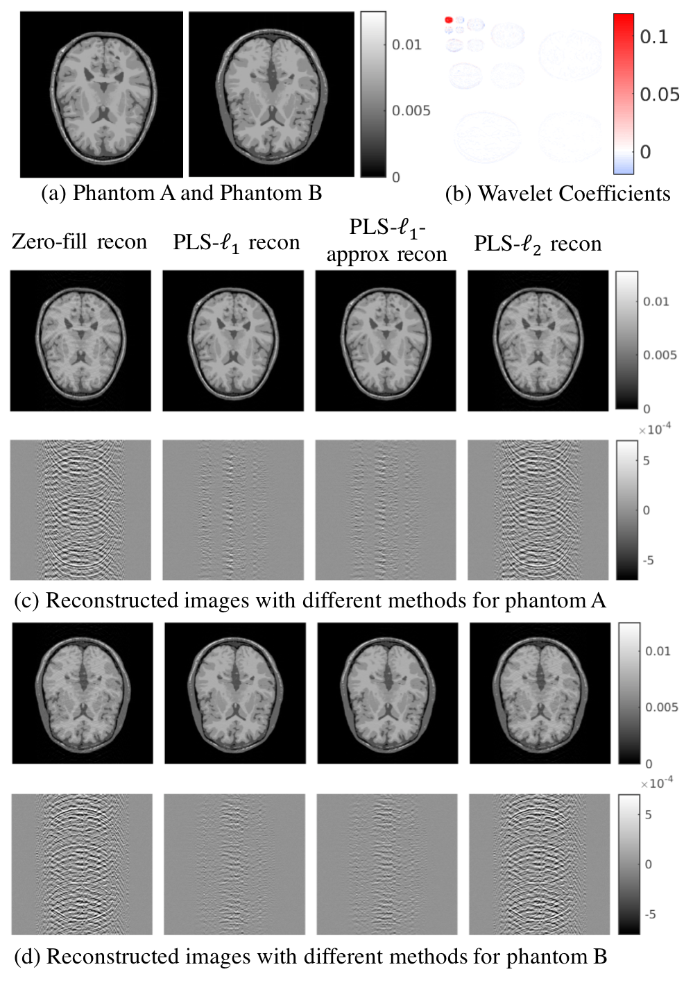
Figure 3: The reconstructed images for two different phantoms (shown in (a)) and different reconstruction methods. Subfigure (b) shows the wavelet coefficients for the first phantom. Zeros are denoted by the white color. The widespread white region in the wavelet image demonstrates the sparseness in the wavelet domain. Subfigures (c) and (d) show reconstructed images for the two different phantoms. In both (c) and (d), the first row shows the reconstructed images and the second row shows the difference images between the reconstructed images and the true phantom. In each row, from left to right are zero-filling reconstruction, PLS-$\ell_{1}$ reconstruction, PLS-$\ell_{1}-approx$ reconstruction, and PLS-$\ell_{2}$ reconstruction.

The estimates above were computed from computer-simulated data corresponding to a stylized two-dimensional (2D) MRI example in which the imaging system sampled random lines from k-space. Two different head phantoms were employed to represent the to-be-imaged object, which are displayed in Figs. 3-(a). The sparsity of the phantom in the wavelet domain is demonstrated in Figs. 3-(b). Additional details regarding these numerical phantoms are described later in Sec. V-A. To demonstrate the impact of under-sampling in the simulated measurement data, images were reconstructed by zero-filling the missing k-space regions and applying an inverse 2D discrete Fourier transform (DFT). This method is also known as the pseudoinverse method [18]. The resulting images, shown in the first rows and second columns of Figs. 3-(c) and (d), contain aliasing artifacts. The artifacts are clearly visible in the difference images that are shown in the second rows and first columns of Figs. 3-(c) and (d), which were formed by subtracting the reconstructed images from the corresponding true phantoms.

The images corresponding to the PLS-$\ell_{1}$, PLS-$\ell_{1}-approx$, and PLS-$\ell_{2}$ estimates are displayed in the second, third, and fourth columns of the top rows in Figs. 3-(c) and (d). The corresponding difference images are shown in the lower row of each subfigure. Note that the PLS-$\ell_{2}$ estimate contains significant artifacts that are similar in nature to those produced by the zero-filling-inverse DFT approach. Tuning the regularization parameter did not change this observation. On the other hand, the PLS-$\ell_{1}$ and PLS-$\ell_{1}-approx$ estimates have significantly reduced artifact levels as compared to the PLS-$\ell_{2}$ estimate. This is expected, as sparsity-promoting regularization methods are known to be more effective for mitigating data incompleteness than $\ell_{2}$-based methods. Moreover, it is observed that the PLS-$\ell_{1}$ and PLS-$\ell_{1}-approx$ image estimates are nearly indistinguishable. Namely, the magnitude and spatial distribution of errors in these two image estimates, as reflected in the difference images, are almost the same. This suggests that the approximated prior in Eq. (14) promotes (wavelet-domain) sparsity is a manner very similar to how the exact sparse prior Eq. (7) does. This is evidence of the accuracy of the variational approximation that underlies the proposed method for computing the SDO test statistic.

V System Rank-Ordering Study

An important application of numerical observers is the rank-ordering of imaging system or data-acquisition designs. In this section, the SDO will be applied to rank four different data-acquisition designs via performance in a tumor-detection task in a stylized 2D MRI example.

V-A Study Design

Four MRI data-acquisition designs were considered for comparison. Each design sampled different 256 phase-encoding lines that were uniformly-spaced between the highest positive (+$k_{\text{max}}=500$ m^-1) and negative (-$k_{\text{max}}=-500$ m^-1) spatial frequencies, as shown in Fig. 4. Among the four candidate patterns, the full scan (FS) sampling pattern (not shown) comprises all 256 phase-encoding lines in k-space and serves as a reference. All three of other patterns are half-scan schemes that each contain 144 sampled phase-encoding lines. The uniform half-scan (UH) sampling pattern comprises 72 lines within a low-frequency region of k-space with an 72 additional lines uniformly spaced in the rest of k-space; the random half-scan (RH) sampling pattern comprises the same low-frequency 72 lines and 72 additional lines sampled randomly; the low-pass half-scan (LH) sampling pattern has all 144 lines in a low-frequency region.

(a) UH

(b) RH

(c) LH

Figure 4: Sampling patterns of half-scan candidate data-acquisition designs: (a) UH: uniform half-scan; (b) RH: random half-scan; (c) LH: low-pass half-scan. The white lines are the sampled phase-encoding lines in k-space while the black lines are un-sampled. The center of the image corresponds to low-frequency components.

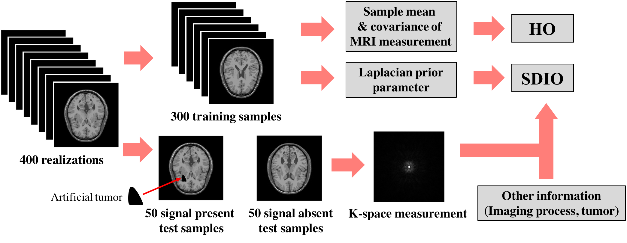
(a)

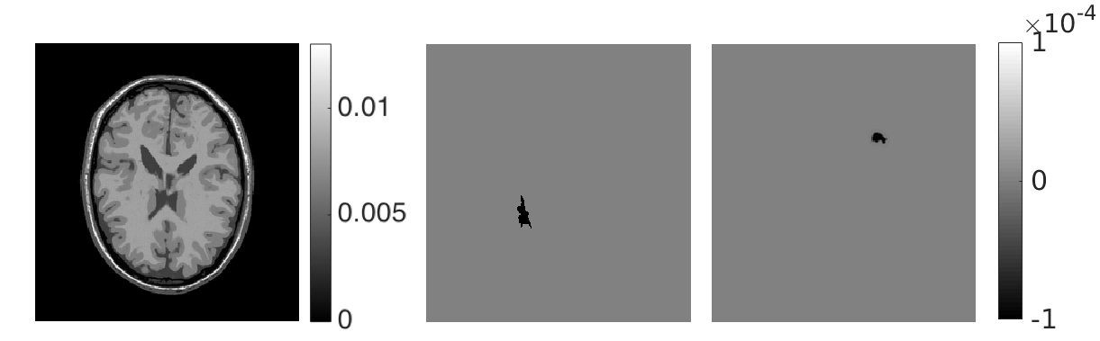
(b)

Figure 5: (a) The flowchart of generating the simulated data for the observers. (b) From left to right: a sample background head phantom, tumor phantom 1, tumor phantom 2.

The process of ranking the candidate designs is illustrated in Fig. 5(a). Numerical real-valued brain phantoms were obtained from an online phantom library[39]. These phantoms were designed to represent reconstructed T1-weighted brain images while considering some limitations of the imaging process such as the partial volume effect and limited receiver bandwidth. This means that a zoomed-in region of the phantom may contain subtle features that resemble artifacts; however, within the context of our study these will simply represent components of the phantom. Out of the available 20 digital 3D brain phantoms, which depicted normal brain anatomies, we extracted 400 2D brain slices that each contained $256\times 256$ pixels with each pixel having a dimension of 1 mm. The phantoms were organized into two sets: 300 phantoms were randomly chosen to form a training set and the remaining 100 phantoms formed a testing set. The samples in the training set were employed to estimate the first and second order statistics required in the Hotelling observer (HO) and the Laplacian parameter $\tau$ for SDO. The 100 testing images were further divided into 50 signal present test images and 50 signal absent test images to assess tumor-detection performance for both the SDO and the HO. To produce the 50 signal present images, a simulated tumor phantom (tumor phantom 1) was generated (Fig. 5(b), middle panel) and superimposed on a slice of the brain phantom. Idealized k-space measurement data were produced corresponding to the four sampling patterns. Zero-mean i.i.d. complex Gaussian noise of standard deviation $\sigma=2\times 10^{-5}$ was added to the measurements to create noisy data sets, generated by creating real-valued Gaussian noise with a standard deviation of $\sigma^{\prime}=\sigma/\sqrt{2}$ for the real and imaginary parts separately. This noise level corresponds to 20% of the maximum value of the tumor signal. Finally, the SDO test statistic was computed by use of the k-space data corresponding to each phantom in the testing set and ROC curves were generated. The implementation details of the SDO test statistical calculation are given in Appendix A. The Hotelling observer implementation follows a standard procedure[36]. All ROC curves were fit based on the semi-parametric binormal model[40]. The area under the curves (AUC) were computed as a figure-of-merit for signal detection performance. The procedure above was repeated by use of second tumor phantom (tumor phantom 2), as shown in Fig. 5(b), right panel. The contrast of this signal was the same as that of the first signal, with only the size, shape, and location of the signal being different. In this second study, the training and testing sets were re-formed by random sampling.

The effect of the training set size on the performance of the numerical observers was considered. In the implementation of the SDO, the sparsifying transform $\mathbf{B}$ was selected to be a four-level Haar wavelet transform. Haar wavelet is the simplest wavelet basis and four-level decomposition is a fair choice for this study where the discretized object size is $256\times 256$. In this case, $\mathbf{B}$ is a square matrix and thus the dimension of the transformed linear space $Q=N=65536$, which is the dimension of the object vector $\mathbf{f}$. The parameter $\tau$ was estimated by use of the training samples as described in Appendix B. It was observed that changing the number of training samples from 1 to 300 lead to a maximum fluctuation of only $0.01$% in the estimated $\tau$ value. This suggests that, in the case considered, the number of training samples did not significantly change the estimated $\tau$ value and hence did not affect strongly the SDO performance. Consequently, here, $\tau$ was estimated from only one training sample. In other situations when the training set comes from multiple sources and has larger ensemble variation, multiple training samples may be necessary to accurately estimate $\tau$; however, as long as the training images are on the same order of magnitude, the required number of training samples remains low because only one parameter needs to be estimated. On the other hand, the number of training samples employed to estimate the background covariance matrix can significantly affect HO performance. In this study, all 300 training samples were utilized for this purpose. For a comparison, a second, limited data situation was simulated by training the HO by use of only 100 training samples.

V-B Rank-Ordering of Data Acquisition Designs

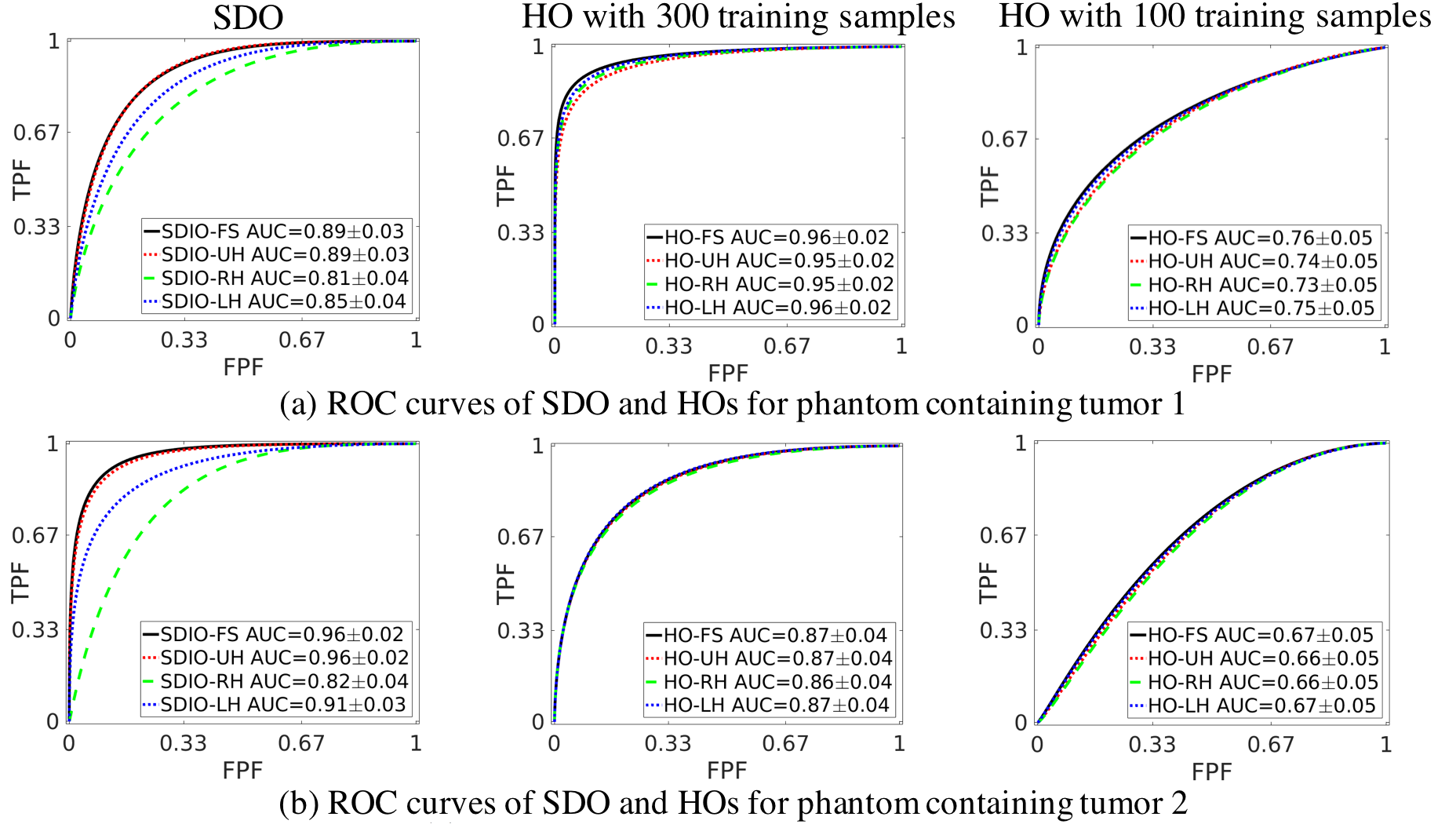
Figure 6: ROC curves and AUC values for different data-acquisition designs. Subfigures (a) and (b) correspond to use of phantoms that contain tumors 1 and 2. In each subfigure, the numerical observers employed were the SDO (left panel), HO with 300 training images (middle panel), and HO with 100 training images (right panel). The curves corresponding to different colors correspond to the different designs: black: full scan (FS); red: uniform half-scan (UH); green: random half-scan (RH); blue: low-pass half-scan (LH). The SDO yields a larger separation between ROC curves than does the HO, which facilitates their rank ordering.

The ROC curves generated for each of the four candidate data-acquisition designs are shown in Fig. 6. Subfigures (a) and (b) correspond to the use of tumor phantom 1 and tumor phantom 2, as described above. As shown in Fig. 6a, the half-scan ROC curves that describe the SDO performance are separated and provide a distinguishable ranking according to the AUC values: FS $\approx$ UH $>$ LH $>$ RH. On the other hand, the ROC curves that describe the HO performance are quite close to each other, and not separated as much as the curves for the SDO. Moreover, the AUC values describing HO performance suggest a different ranking of half-scan designs: FS $>$ LH $>$ UH $>$ RH (HO with 100 training samples) or FS $>$ LH $>$ RH $>$ UH (HO with 300 training samples). The ROC curves in Fig. 6b yield similar observations. However, in that case, the four ROC curves corresponding to the HO appear nearly indistinguishable, so no clear rank-ordering can be achieved.

In summary, it is expected that the FS data-acquisition design should yield the best signal-detection performance, and the results produced by use of both the SDO and HO confirm this. When restricted to a half-scan design, the SDO ranks the the UH as best while the HO ranks the LH as best (when it is still capable of producing a ranking). This demonstrates that the SDO, which utilizes a reconstruction prior, and HO, which ignores image reconstruction entirely, can produce different rank orderings of designs.

V-C Visual Inspection of Images

To gain insights into the quality of the conflicting optimal half-scan data-acquisition designs identified by use of the SDO and HO, images were reconstructed. Firstly, for each of the phantoms, PLS-$\ell_{1}$ image estimates were computed from the k-space data corresponding to the UH and LH data-acquisition designs. As described above, these correspond to the optimal half-scan designs identified by use of the SDO and HO, respectively. The penalty term employed in the PLS-$\ell_{1}$ estimator was defined to be consistent with the sparse object prior in Eq. (7), as described in Sec. IV-B, where the sparsifying transform was the Haar Wavelet transform introduced in Sec. V-A for SDO test statistic calculations. The object was constrained to be real-valued. The reconstructed images are displayed in Fig. 7 and reveal that, in the case of the UH design, the reconstructed tumor signal possesses have high contrast and clear boundaries. On the other hand, in the case of the LH design, the reconstructed tumor signal possesses lower contrast and distorted boundaries. These observations suggest that the UH design that was identified as optimal by the SDO may be a better choice for the specified signal-detection task than the LH design identified by the HO. The structural similarity (SSIM)[41] values, also displayed in Fig. 7, indicate that the images corresponding to the UH design are more similar to the true phantom than those corresponding to the LH design.

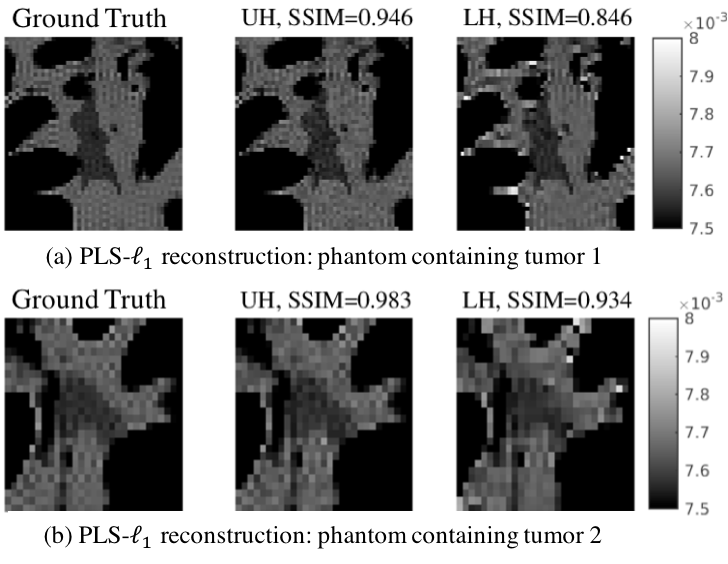
Figure 7: ROIs from images reconstructed by use of the PLS-$\ell_{1}$ estimator. Subfigures (a) and (b) correspond to use of phantoms that contain tumors 1 and 2. In each subfigure, the image in the left panel represents the phantom (ground truth). The images in the center and right panels were reconstructed from data corresponding to the UH and LH designs.

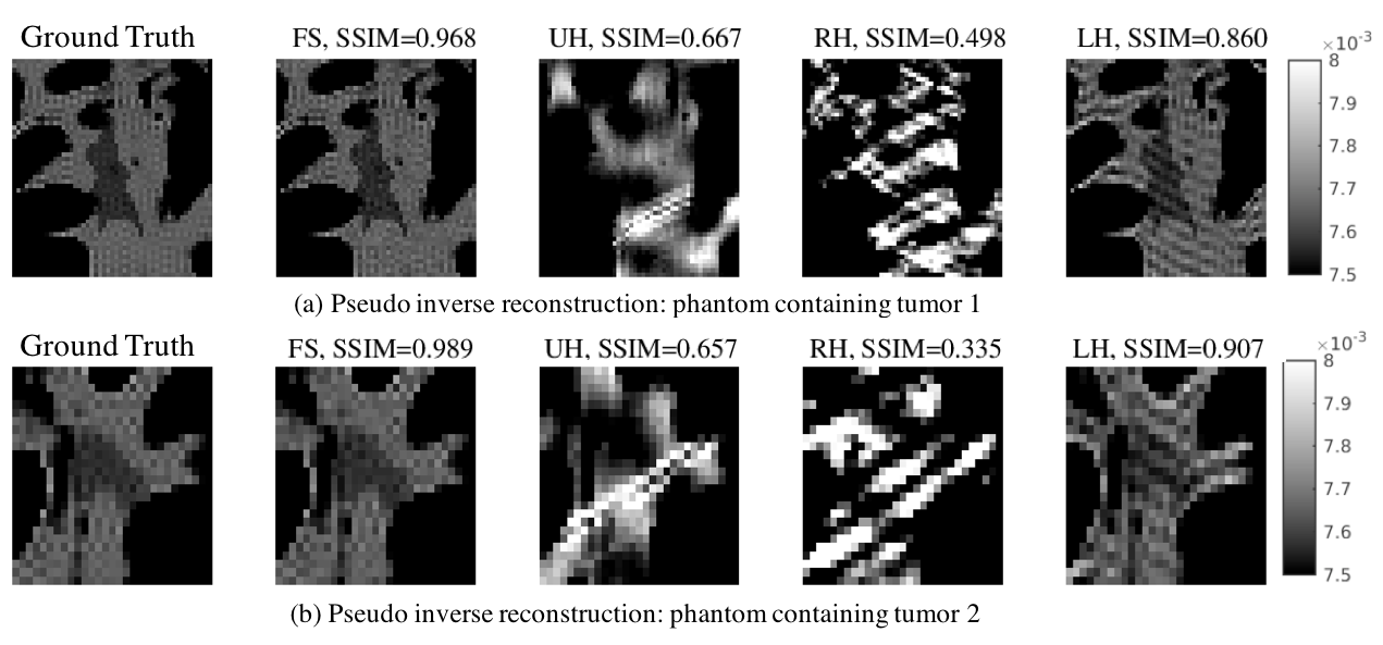
Figure 8: ROIs from images reconstructed by use of the pseudoinverse reconstruction method. Subfigures (a) and (b) correspond to use of phantoms that contain tumors 1 and 2. In each subfigure, the image in the far-left panel represents the phantom (ground truth). The remaining images, from left-to-right, were reconstructed from k-space data corresponding to the FS, UH, RH, and LH, designs, respectively.

To further investigate the role of image reconstruction algorithm on design rank orderings, images were re-reconstructed by use of a pseudoinverse method [18] instead of the sparse reconstruction method. The reconstructed images are displayed in Fig. 8. As observed with the PLS-$\ell_{1}$ estimator and reflected by the SSIM values, the images reconstructed from data corresponding to the FS design were the most similar to the true phantoms. However, the visual appearance rankings of the images corresponding to the half-scan designs are distinct from the the case where the PLS-$\ell_{1}$ estimator was employed. Namely, in terms of visual appearances and SSIM values, the images corresponding to the LH design are now superior to the other designs. Note that the images corresponding to the UH design (the optimal design according to the SDO), are highly distorted and therefore likely to lead to compromised signal-detection performance. This occurs because of a mismatch in the information that is utilized by the SDO and pseudoinverse reconstruction method; the SDO employed information regarding the object sparsity that was not exploited by the pseudoinverse reconstruction method. It should also be noted that the images reconstructed by use of the PLS-$\ell_{1}$ method corresponding to the UH design (Fig. 7a and b, center panels) are more similar to the phantoms than are the images reconstructed by use of the pseudoinverse method (Fig. 8a and b, right-most panel) corresponding to the LH design. These observations support our conjecture that, when attempting to mitigate data incompleteness by use of a sparse image reconstruction method, matching statistical information utilized by the observer and reconstruction method can be advantageous for optimizing system designs.

VI Discussion and conclusion

The SDO represents a new type of numerical observer that will find application in optimizing the performance of modern computed imaging systems that employ sparse reconstruction methods. Unlike a traditional IO that is predicated upon comprehensive statistical knowledge of the class of objects to-be-imaged, the SDO assumes a stochastic and data-driven object model that describes only the sparsity properties of the class of objects. As such, the SDO and sparse reconstruction method both utilize the same statistical information related to the sparsity properties of the class of objects to-be-imaged. This information is already known to be useful for sparse reconstruction methods. As such, the use of the SDO will permit task-specific optimization of data-acquisition and system designs with consideration of the sparse reconstruction method to be employed.

An important contribution of this work was the development and implementation of a method for computing the SDO test statistic for the case of i.i.d. Gaussian measurement noise. To circumvent the computational burden of MCMC methods, a variational method for approximating the required posterior distribution was adopted. Subsequently, the test statistic could be computed semi-analytically; this can reduce computation times by orders of magnitude compared with MCMC methods. To the best of our knowledge, this represents the first application of a variational Bayesian inference method for estimating an likelihood ratio test statistic.

Many existing methods for imaging system optimization prescribe that imaging hardware or data-acquisition designs should be optimized by use of an IO that exploits full statistical knowledge of the measurement noise and class of objects to-be-imaged, without consideration of the reconstruction method [1, 42]. The numerical studies presented in this work suggest that the notion may not always be applicable to modern imaging systems that employ sparse image reconstruction methods. Firstly, in a stylized MRI study, it was demonstrated that the SDO and HO yielded different rank orderings of data-acquisition designs. When a sparse reconstruction method was employed, the optimal design predicted by the SDO resulted in reconstructed images with decreased artifact levels as compared to the images corresponding to the optimal HO-specified design. Moreover, it is possible that the optimal system design can change when the sparse reconstruction method is changed. Secondly, from the rank ordered data-acquisition designs described above, images were re-reconstructed by use of a pseudo inverse method instead of the sparse reconstruction method. In this case, the optimal design predicted by the HO resulted in reconstructed images with significantly decreased artifact levels as compared to the images corresponding to the optimal SDO-specified design. These studies suggest that it can be important to consider the image reconstruction method to be employed when adopting a numerical observer to optimize the performance of computed imaging systems that employ sparse reconstruction methods. More specifically, in such applications, it can be important for the numerical observer and reconstruction method to be statistically matched.

There remain numerous topics for future investigation. In terms of technical developments, there is a need to extend the presented work to address other measurement noise models such as a generalized Gaussian noise model or a Poisson noise model. To accomplish this, additional approximations may be required and the impact of the approximations on the accuracy of estimated posterior distribution should be studied systematically. It may also be important to generalize the method to address more complicated signal-detection tasks, such as signal-known-statistically tasks. To further reduce the computational burden of the method for use with three-dimensional imaging systems, a channelized version [5] of the SDO can also be explored. Finally, it will be important to identify real-world applications for which imaging system performance can be improved by use of the SDO.

Appendix A Computation of the SDO Test Statistic

The SDO test statistic was computed as described by the pseudocode presented in Alg. 1. First, the parameter $\tau$ for the Laplacian distribution was estimated based on the statistics of the training samples. Second, for each test sample, $\gamma_{i}$ ($i=1,2,...,Q$) values were chosen to minimize the KL-divergence between the approximated Gaussian distribution in Eq. (15) and the true posterior distribution in Eq. (5). The optimization problem can be solved by a double loop algorithm [35] shown in Alg. 2. The iterations should stop when the $\gamma_{i}$ values converge. In our implementation, a fixed maximum iteration number $k_{0}$ was empirically selected to be 16. Finally, the likelihood ratios were calculated.

Note that a real-valued object model was assumed in this study. In other words, $\mathbf{f}\in\mathbb{R}^{N}$. Thus in the double-loop algorithm, the variance vector $\mathbf{z}$, object vector $\mathbf{f}$ and the matrix $\boldsymbol{\Gamma}$ corresponding the approximated prior are all real-valued. Extension to complex-valued object models is also possible by modeling the real and imaginary components of the objects separately by different Laplacian priors. More details are available in literature[33, 35].

Algorithm 1 SDO test statistic calculation for one test sample

1:  Estimate the parameter $\tau$ for the Laplacian distribution based on the test samples

2:  Calculate the $\gamma_{i}^{(0)}$ ($i=1,2,...,Q$) values by use of the double loop algorithm

3:  Solve the optimization problem in Eq. (24)

4:  Calculate the likelihood ratio based on Eq. (23)

Algorithm 2 Double loop algorithm

1:  Initialize $\gamma_{i}^{(0)}$ ($i=1,2,...,Q$) to a large number ($1000$ in our implementation) and form the diagonal matrix $\boldsymbol{\Gamma}^{(0)}$

2:  for $k$=1,2,…$k_{0}$ do

3:     Calculate $\mathbf{A}^{(k)}=\mathbf{B}^{\dagger}(\boldsymbol{\Gamma}^{(k-1)})^{-1}\mathbf{B}+\mathbf{H}^{\dagger}\boldsymbol{\Sigma}_{n}^{-1}\mathbf{H}$

4:     Calculate $\mathbf{z}^{(k)}=$ diag${}^{-1}(\mathbf{B}[\mathbf{A}^{(k)}]^{-1}\mathbf{B}^{\dagger})$

5:     Solve the optimization problem using a gradient descent algorithm (the inner-loop)

$$\mathbf{f}^{(k)}=\arg\min_{\mathbf{f}}\sigma^{-2}\|\mathbf{Hf-g}\|^{2}+2\tau\sqrt{z_{i}^{(k)}+[\mathbf{Bf}]_{i}^{2}}$$

6:     Calculate $[\gamma^{(k)}]_{i}=\tau^{-1}\sqrt{z_{i}^{(k)}+[\mathbf{Bf}^{(k)}]_{i}^{2}}$. Form the diagonal matrix $\boldsymbol{\Gamma}^{(k)}$

7:  end for

Appendix B Estimation of Laplacian Distribution Parameter

The Laplacian distribution parameter $\tau$ was chosen based on a training dataset. For the sparse prior assumed in Eq. (7), the variance of the Laplacian distribution is $2/\tau^{2}$. Thus, the Laplacian parameter was specified as

$$\tau=\sqrt{2/\text{var}(w)},$$ (32)

where $w$ denotes an element in the transformed sparse vector $\mathbf{w}$ obtained by Eq. (6), and var$(w)$ denote the sample variance of $w$, estimated by

$$\text{var}(w)=E(w^{2})-E(w)^{2}.$$ (33)

Here, $E(w)$ and $E(w^{2})$ denote the expectations of $w$ and $w^{2}$, respectively. Both of the expectations were empirically estimated based on a pool of sparse vector element samples formed by stacking together all the transformed vector elements from training images.

In our study, the wavelet transform was employed as the sparsifying transform. Thus, $w$ denotes a wavelet coefficient. Note that in this case, there can be outliers that lead to underestimation of $\tau$. To circumvent this, the wavelet coefficients were subjected to a threshold that removed outliers prior to estimating $\tau$ via Eq. (32). The threshold value was selected empirically. We varied $\tau$ within a range of values that yielded visually reasonable reconstructed images (data not shown); the conclusions related to the ranking of the data-acquisition designs was not altered.

Appendix C Inversion of a Large Matrix

The inversion of a large matrix can be a bottleneck in the computation of numerical observers [43]. In the present case, the inversion of $\mathbf{A}$ is the most computationally challenging task in the double loop algorithm. The sparsifying matrix $\mathbf{B}$ is full rank and $\mathbf{B}^{-1}=\mathbf{B}^{\dagger}$. Thus we have $\mathbf{B}[\mathbf{A}^{(k)}]^{-1}\mathbf{B}^{\dagger}=[\mathbf{B}\mathbf{A}^{(k)}\mathbf{B}^{\dagger}]^{-1}$. Denote $\mathbf{C}=\mathbf{B}\mathbf{A}^{(k)}\mathbf{B}^{\dagger}$. It follows that $\mathbf{C}=[(\boldsymbol{\Gamma}^{(k-1)})^{-1}+\mathbf{B}\mathbf{H}^{\dagger}\boldsymbol{\Sigma}_{n}^{-1}\mathbf{H}\mathbf{B}^{\dagger}]^{-1}$. Thus, steps 3 and 4 in Alg. 2 can be combined into one step, where the matrix $\mathbf{C}$ is inverted, and only the diagonal elements of the inverse matrix are needed. In this study, a parallel sparse direct solver called MUMPS [44, 45] was employed for this calculation. For the MRI application in our study, the matrix $\mathbf{C}$ contains many small values; as such, the $\mathbf{C}$ matrix can be thresholded to form a new sparse matrix $\mathbf{C}_{\text{approx}}$ that closely approximates the original $\mathbf{C}$ matrix. Consequently, the inverse of the approximated matrix $(\mathbf{C}_{\text{approx}})^{-1}$ can be regarded as a close approximation of the original matrix’s inverse $\mathbf{C}^{-1}$. However, $\mathbf{C}_{\text{approx}}$ is much easier to invert because it is sparse. The MUMPS solver is designed purposefully to compute any desired element in the inverse of a sparse matrix and thus was employed to obtain the diagonal elements of $(\mathbf{C}_{\text{approx}})^{-1}$. In our study, a threshold of $0.01$ was employed. In practice, the diagonal elements of $\mathbf{C}$ are preserved in $\mathbf{C}_{\text{approx}}$ to prevent solving an ill-conditioned inverse problem.

Appendix D Derivation of SDO test statistics (Eq. (18))

Below, the derivation of the SDO test statistic considered in this work is provided. As mentioned in Sec. III-B, by approximating the Laplacian priors using parameterized Gaussian priors, the corresponding approximated posterior distribution is given by Eq. (15):

$$P(\mathbf{f}_{b}|\mathbf{g},\mathcal{H}_{0})_{Q(\mathbf{f}_{b};\boldsymbol{\gamma})}=Z_{a}^{-1}\mathcal{N}(\mathbf{g}|\mathbf{H}\mathbf{f}_{b},\sigma^{2}\mathbf{I})\exp\left(-{\mathbf{w}^{T}\boldsymbol{\Gamma}^{-1}\mathbf{w}}/2\right)$$

$$=Z_{a}^{-1}(2\pi)^{\frac{n}{2}}|\boldsymbol{\Sigma}_{n}|^{\frac{1}{2}}\exp\left\{-\frac{1}{2}(\mathbf{g}-\mathbf{Hf}_{b})^{\dagger}\boldsymbol{\Sigma}_{n}^{-1}(\mathbf{g}-\mathbf{Hf}_{b})\right\}\times\exp\left(\frac{1}{2}\mathbf{f}_{b}^{\dagger}\mathbf{B}^{\dagger}\boldsymbol{\hat{\Gamma}}(\mathbf{g})^{-1}\mathbf{B}\mathbf{f}_{b}\right)$$

$$\propto\exp\left\{-\frac{1}{2}(\mathbf{g}-\mathbf{Hf}_{b})^{\dagger}\boldsymbol{\Sigma}_{n}^{-1}(\mathbf{g}-\mathbf{Hf}_{b})-\frac{1}{2}\mathbf{f}_{b}^{\dagger}\mathbf{B}^{\dagger}\boldsymbol{\hat{\Gamma}}(\mathbf{g})^{-1}\mathbf{Bf}_{b}\right\}$$

$$\propto\exp\left\{-\frac{1}{2}\left[\mathbf{g}\boldsymbol{\Sigma}_{n}^{-1}\mathbf{g}-2\mathbf{g}^{\dagger}\boldsymbol{\Sigma}_{n}^{-1}\mathbf{Hf}_{b}+\mathbf{f}_{b}^{\dagger}\mathbf{H}^{\dagger}\boldsymbol{\Sigma}_{n}^{-1}\mathbf{Hf}_{b}+\mathbf{f}_{b}^{\dagger}\mathbf{B}^{\dagger}\boldsymbol{\hat{\Gamma}}(\mathbf{g})^{-1}\mathbf{Bf}_{b}\right]\right\}$$

$$\propto\exp\left(-\frac{1}{2}\mathbf{g}^{\dagger}\boldsymbol{\Sigma}_{n}^{-1}\mathbf{g}\right)\exp\left\{-\frac{1}{2}\left[\mathbf{f}_{b}^{\dagger}\mathbf{H}^{\dagger}\boldsymbol{\Sigma}_{n}^{-1}\mathbf{H}\mathbf{f}_{b}-2\mathbf{g}^{\dagger}\boldsymbol{\Sigma}_{n}^{-1}\mathbf{Hf}_{b}+\mathbf{f}_{b}^{\dagger}\mathbf{B}^{\dagger}\boldsymbol{\hat{\Gamma}}(\mathbf{g})^{-1}\mathbf{Bf}_{b}\right]\right\}$$

$$\propto\exp\left\{-\frac{1}{2}\left[\mathbf{f}_{b}^{\dagger}\left(\mathbf{H}^{\dagger}\boldsymbol{\Sigma}_{n}^{-1}\mathbf{H}+\mathbf{B}^{\dagger}\boldsymbol{\hat{\Gamma}}(\mathbf{g})^{-1}\mathbf{B}\right)\mathbf{f}_{b}-2\mathbf{g}^{\dagger}\boldsymbol{\Sigma}_{n}^{-1}\mathbf{Hf}_{b}\right]\right\}$$

$$\propto\exp\left[-\frac{1}{2}(\mathbf{f}_{b}-\mathbf{f}_{x})^{\dagger}\boldsymbol{\Sigma}(\mathbf{g})^{-1}(\mathbf{f}_{b}-\mathbf{f}_{x})\right],$$ (34)

where

$$\left\{\begin{array}[]{l}\boldsymbol{\Sigma}(\mathbf{g})=\left[\mathbf{H}^{\dagger}\boldsymbol{\Sigma}_{n}^{-1}\mathbf{H}+\mathbf{B}^{\dagger}\boldsymbol{\hat{\Gamma}}(\mathbf{g})^{-1}\mathbf{B}\right]^{-1}\\ \mathbf{f}_{x}=\boldsymbol{\Sigma}(\mathbf{g})^{\dagger}\mathbf{H}^{\dagger}\boldsymbol{\Sigma}_{n}^{-1}\mathbf{g}\end{array}\right.$$ (35)

and terms independent of $\mathbf{f}_{b}$ are omitted in the derivation. Based on the fact that the distribution is normalized,

$$P(\mathbf{f}_{b}|\mathbf{g},\mathcal{H}_{0})_{Q(\mathbf{f}_{b};\boldsymbol{\gamma})}=Z_{1}^{-1}\exp\left[-\frac{1}{2}(\mathbf{f}_{b}-\mathbf{f}_{x})^{\dagger}\boldsymbol{\Sigma}(\mathbf{g})^{-1}(\mathbf{f}_{b}-\mathbf{f}_{x})\right],$$ (36)

where $Z_{1}=(2\pi)^{\frac{n}{2}}\left|\boldsymbol{\Sigma}(\mathbf{g})\right|^{\frac{1}{2}}$.

The BKE likelihood ratio is given by Eq. (11):

$$\Lambda_{BKE}(\mathbf{g}|\mathbf{f}_{b})=\exp\left[\left(\mathbf{g}-\mathbf{Hf}_{b}-\frac{1}{2}\mathbf{Hf}_{s}\right)^{\dagger}\boldsymbol{\Sigma}_{n}^{-1}\mathbf{Hf}_{s}\right].$$ (37)

By taking Eq. (36) and Eq. (37) into the integral form of ideal observer test statistics in Eq. (4), one obtains

$$\Lambda(\mathbf{g})=\int\mathop{}\!\mathrm{d}\mathbf{f}_{b}\Lambda_{BKE}(\mathbf{g}|\mathbf{f}_{b})P(\mathbf{f}_{b}|\mathbf{g},\mathcal{H}_{0})_{Q(\mathbf{f}_{b};\boldsymbol{\gamma})}$$

$$=\int\mathop{}\!\mathrm{d}\mathbf{f}_{b}\exp\left\{\left(\mathbf{g}-\mathbf{Hf}_{b}-\frac{1}{2}\mathbf{Hf}_{s}\right)^{\dagger}\boldsymbol{\Sigma}_{n}^{-1}\mathbf{Hf}_{s}\right\}Z_{1}^{-1}\exp\left\{-\frac{1}{2}(\mathbf{f}_{b}-\mathbf{f}_{x})^{\dagger}\boldsymbol{\Sigma}(\mathbf{g})^{-1}(\mathbf{f}_{b}-\mathbf{f}_{x})\right\}$$

$$=Z_{1}^{-1}\int\mathop{}\!\mathrm{d}\mathbf{f}_{b}\exp\left\{\left(\mathbf{g}-\frac{1}{2}\mathbf{Hf}_{s}\right)^{\dagger}\boldsymbol{\Sigma}_{n}^{-1}\mathbf{Hf}_{s}-(\mathbf{Hf}_{b})^{\dagger}\boldsymbol{\Sigma}_{n}^{-1}\mathbf{Hf}_{s}\right\}$$

$$\qquad\exp\left\{-\frac{1}{2}\left[\mathbf{f}_{b}^{\dagger}\boldsymbol{\Sigma}(\mathbf{g})^{-1}\mathbf{f}_{b}-\mathbf{f}_{b}^{\dagger}\boldsymbol{\Sigma}(\mathbf{g})^{-1}\mathbf{f}_{x}-\mathbf{f}_{x}^{\dagger}\boldsymbol{\Sigma}(\mathbf{g})^{-1}\mathbf{f}_{b}+\mathbf{f}_{x}^{\dagger}\boldsymbol{\Sigma}(\mathbf{g})^{-1}\mathbf{f}_{x}\right]\right\}$$

$$=Z_{1}^{-1}\exp\left[(\mathbf{g}-\frac{1}{2}\mathbf{Hf}_{s})^{\dagger}\boldsymbol{\Sigma}_{n}^{-1}\mathbf{Hf}_{s}\right]\exp\left[-\frac{1}{2}\mathbf{f}_{x}^{\dagger}\boldsymbol{\Sigma}(\mathbf{g})^{-1}\mathbf{f}_{x}\right]$$

$$\qquad\times\int\mathop{}\!\mathrm{d}\mathbf{f}_{b}\exp\left\{-\frac{1}{2}\left[\mathbf{f}_{b}^{\dagger}\boldsymbol{\Sigma}(\mathbf{g})^{-1}\mathbf{f}_{b}-2\mathbf{f}_{x}^{\dagger}\boldsymbol{\Sigma}(\mathbf{g})^{-1}\mathbf{f}_{b}+2(\mathbf{Hf}_{s})^{\dagger}\boldsymbol{\Sigma}_{n}^{-1}\mathbf{Hf}_{b}\right]\right\}.$$ (38)

Let $A=\exp\left[(\mathbf{g}-\frac{1}{2}\mathbf{Hf}_{s})^{\dagger}\boldsymbol{\Sigma}_{n}^{-1}\mathbf{Hf}_{s}\right]\exp\left[-\frac{1}{2}\mathbf{f}_{x}^{\dagger}\boldsymbol{\Sigma}(\mathbf{g})^{-1}\mathbf{f}_{x}\right]$:

$$\centering\Lambda(\mathbf{g})\@add@centering =Z_{1}^{-1}A\int\mathop{}\!\mathrm{d}\mathbf{f}_{b}\exp\left\{-\frac{1}{2}\left[\mathbf{f}_{b}^{\dagger}\boldsymbol{\Sigma}(\mathbf{g})^{-1}\mathbf{f}_{b}-2\left(\mathbf{f}_{x}^{\dagger}\boldsymbol{\Sigma}(\mathbf{g})^{-1}-(\mathbf{Hf}_{s})^{\dagger}\boldsymbol{\Sigma}_{n}^{-1}\mathbf{H}\right)\mathbf{f}_{b}\right]\right\}$$

$$=Z_{1}^{-1}A\int\mathop{}\!\mathrm{d}\mathbf{f}_{b}\exp\left\{-\frac{1}{2}\left[\mathbf{f}_{b}^{\dagger}\boldsymbol{\Sigma}(\mathbf{g})^{-1}\mathbf{f}_{b}-2\mathbf{f}_{y}^{\dagger}\boldsymbol{\Sigma}(\mathbf{g})^{-1}\mathbf{f}_{b}\right]\right\}$$ (39)

where $\mathbf{f}_{y}=\mathbf{f}_{x}-\boldsymbol{\Sigma}(\mathbf{g})^{\dagger}\mathbf{H}^{\dagger}\boldsymbol{\Sigma}_{n}^{-1}\mathbf{Hf}_{s}$. Equation (39) can further be written as:

$$\Lambda(\mathbf{g}) =Z_{1}^{-1}A\int\mathop{}\!\mathrm{d}\mathbf{f}_{b}\exp\left\{-\frac{1}{2}\left[\mathbf{f}_{b}^{\dagger}\boldsymbol{\Sigma}(\mathbf{g})^{-1}\mathbf{f}_{b}-2\mathbf{f}_{y}^{\dagger}\boldsymbol{\Sigma}(\mathbf{g})^{-1}\mathbf{f}_{b}+\mathbf{f}_{y}^{\dagger}\boldsymbol{\Sigma}(\mathbf{g})^{-1}\mathbf{f}_{y}\right]\right\}\exp\left[\frac{1}{2}\mathbf{f}_{y}^{\dagger}\boldsymbol{\Sigma}(\mathbf{g})^{-1}\mathbf{f}_{y}\right]$$

$$=Z_{1}^{-1}A\exp\left[\frac{1}{2}\mathbf{f}_{y}^{\dagger}\boldsymbol{\Sigma}(\mathbf{g})^{-1}\mathbf{f}_{y}\right]\times\int\mathop{}\!\mathrm{d}\mathbf{f}_{b}\exp\left[-\frac{1}{2}(\mathbf{f}_{b}-\mathbf{f}_{y})^{\dagger}\boldsymbol{\Sigma}(\mathbf{g})^{-1}(\mathbf{f}_{b}-\mathbf{f}_{y})\right]$$

$$=A\exp\left[\frac{1}{2}\mathbf{f}_{y}^{\dagger}\boldsymbol{\Sigma}(\mathbf{g})^{-1}\mathbf{f}_{y}\right],$$ (40)

Therefore, Eq. (40) can be further simplified as:

$$\Lambda(\mathbf{g})=\exp\Biggl{\{} (\mathbf{g}-\frac{1}{2}\mathbf{Hf}_{s})^{\dagger}\boldsymbol{\Sigma}_{n}^{-1}\mathbf{Hf}_{s}+\frac{1}{2}\big{[}(\mathbf{g}-\mathbf{Hf}_{s})^{\dagger}\boldsymbol{\Sigma}_{n}^{-1}\mathbf{H}\boldsymbol{\Sigma}(\mathbf{g})\mathbf{H}^{\dagger}\boldsymbol{\Sigma}_{n}^{-1}(\mathbf{g}-\mathbf{Hf}_{s})-\mathbf{g}^{\dagger}\boldsymbol{\Sigma}_{n}^{-1}\mathbf{H}\boldsymbol{\Sigma}(\mathbf{g})\mathbf{H}^{\dagger}\boldsymbol{\Sigma}_{n}^{-1}\mathbf{g}\big{]}\Biggr{\}}$$

$$=\exp\biggl{\{} (\mathbf{g}-\frac{1}{2}\mathbf{Hf}_{s})^{\dagger}[\mathbf{I}-\boldsymbol{\Sigma}_{n}^{-1}\mathbf{H}\boldsymbol{\Sigma}(\mathbf{g})\mathbf{H}^{\dagger}]\boldsymbol{\Sigma}_{n}^{-1}\mathbf{Hf}_{s}\biggr{\}},$$ (41)

which is same as Eq. (18).

References

- [1] H. H. Barrett and K. J. Myers, Foundations of Image Science. John Wiley & Sons, 2013.
- [2] C. E. Metz, R. F. Wagner, D. G. Brown, R. M. Nishikawa, K. J. Myers et al., “Toward consensus on quantitative assessment of medical imaging systems,” Medical Physics, vol. 22, no. 7, pp. 1057–1061, 1995.
- [3] W. Vennart, “ICRU Report 54: Medical imaging - the assessment of image quality: Isbn 0-913394-53-x. april 1996, maryland, usa,” 1997.
- [4] R. F. Wagner and D. G. Brown, “Unified SNR analysis of medical imaging systems,” Physics in Medicine and Biology, vol. 30, no. 6, p. 489, 1985.
- [5] X. He and S. Park, “Model observers in medical imaging research,” Theranostics, vol. 3, no. 10, p. 774, 2013.
- [6] G. J. Gang, J. W. Stayman, T. Ehtiati, and J. H. Siewerdsen, “Task-driven image acquisition and reconstruction in cone-beam ct,” Physics in Medicine and Biology, vol. 60, no. 8, p. 3129, 2015.
- [7] E. Y. Sidky and X. Pan, “In-depth analysis of cone-beam ct image reconstruction by ideal observer performance on a detection task,” in Nuclear Science Symposium Conference Record, 2008. NSS’08. IEEE. IEEE, 2008, pp. 5161–5165.
- [8] E. Clarkson and H. H. Barrett, “Approximations to ideal-observer performance on signal-detection tasks,” Applied Optics, vol. 39, no. 11, pp. 1783–1793, 2000.
- [9] A. A. Sanchez, E. Y. Sidky, and X. Pan, “Task-based optimization of dedicated breast ct via hotelling observer metrics,” Medical Physics, vol. 41, no. 10, 2014.
- [10] J. A. Swets, Signal detection theory and ROC analysis in psychology and diagnostics: Collected papers. Psychology Press, 2014.
- [11] W. S. Geisler, “Ideal observer analysis,” The visual neurosciences, vol. 10, no. 7, pp. 12–12, 2003.
- [12] Z. Liu, D. C. Knill, and D. Kersten, “Object classification for human and ideal observers,” Vision Research, vol. 35, no. 4, pp. 549–568, 1995.
- [13] M. A. Kupinski, E. Clarkson, J. W. Hoppin, L. Chen, and H. H. Barrett, “Experimental determination of object statistics from noisy images,” JOSA A, vol. 20, no. 3, pp. 421–429, 2003.
- [14] K. Gross, M. A. Kupinski, and J. Y. Hesterman, “A fast model of a multiple-pinhole spect imaging system,” in Proc. of SPIE Vol, vol. 5749, 2005, p. 119.
- [15] C. G. Graff, T. Flohr, and J. Luo, “A new, open-source, multi-modality digital breast phantom,” Physics of Medical Imaging SPIE, p. 978309, 2016.
- [16] M. A. Kupinski, J. W. Hoppin, E. Clarkson, and H. H. Barrett, “Ideal observer computation in medical imaging with use of Markov-chain Monte Carlo techniques,” JOSA A, vol. 20, no. 3, pp. 430–438, 2003.
- [17] X. He, B. S. Caffo, and E. C. Frey, “Toward realistic and practical ideal observer (io) estimation for the optimization of medical imaging systems,” IEEE Transactions on Medical Imaging, vol. 27, no. 10, pp. 1535–1543, 2008.
- [18] M. Lustig, D. Donoho, and J. M. Pauly, “Sparse MRI: The application of compressed sensing for rapid mr imaging,” Magnetic Resonance in Medicine, vol. 58, no. 6, pp. 1182–1195, 2007.
- [19] M. Lustig, D. L. Donoho, J. M. Santos, and J. M. Pauly, “Compressed sensing MRI,” IEEE Signal Processing Magazine, vol. 25, no. 2, pp. 72–82, 2008.
- [20] S. Ramani and J. A. Fessler, “An accelerated iterative reweighted least squares algorithm for compressed sensing MRI,” in Biomedical Imaging: From Nano to Macro, 2010 IEEE International Symposium. IEEE, 2010, pp. 257–260.
- [21] E. Y. Sidky and X. Pan, “Image reconstruction in circular cone-beam computed tomography by constrained, total-variation minimization,” Physics in Medicine and Biology, vol. 53, no. 17, p. 4777, 2008.
- [22] J. Bian, J. H. Siewerdsen, X. Han, E. Y. Sidky, J. L. Prince, C. A. Pelizzari, and X. Pan, “Evaluation of sparse-view reconstruction from flat-panel-detector cone-beam ct,” Physics in Medicine and Biology, vol. 55, no. 22, p. 6575, 2010.
- [23] J. Stayman, W. Zbijewski, Y. Otake, A. Uneri, S. Schafer, J. Lee, J. Prince, and J. Siewerdsen, “Penalized-likelihood reconstruction for sparse data acquisitions with unregistered prior images and compressed sensing penalties,” in Proc. SPIE, vol. 7961, 2011, p. 79611L.
- [24] H. H. Barrett, C. K. Abbey, and E. Clarkson, “Objective assessment of image quality. iii. roc metrics, ideal observers, and likelihood-generating functions,” JOSA A, vol. 15, no. 6, pp. 1520–1535, 1998.
- [25] M. Elad, M. A. Figueiredo, and Y. Ma, “On the role of sparse and redundant representations in image processing,” Proceedings of the IEEE, vol. 98, no. 6, pp. 972–982, 2010.
- [26] J.-L. Starck, F. Murtagh, and J. M. Fadili, Sparse Image and Signal Processing: Wavelets, Curvelets, Morphological diversity. Cambridge university press, 2010.
- [27] M. W. Seeger, “Bayesian inference and optimal design for the sparse linear model,” Journal of Machine Learning Research, vol. 9, no. Apr, pp. 759–813, 2008.
- [28] M. W. Seeger and H. Nickisch, “Large scale bayesian inference and experimental design for sparse linear models,” SIAM Journal on Imaging Sciences, vol. 4, no. 1, pp. 166–199, 2011.
- [29] C. W. Fox and S. J. Roberts, “A tutorial on variational bayesian inference,” Artificial intelligence review, pp. 1–11, 2012.
- [30] D. G. Tzikas, A. C. Likas, and N. P. Galatsanos, “The variational approximation for bayesian inference,” IEEE Signal Processing Magazine, vol. 25, no. 6, pp. 131–146, 2008.
- [31] M. W. Seeger and D. P. Wipf, “Variational bayesian inference techniques,” IEEE Signal Processing Magazine, vol. 27, no. 6, pp. 81–91, 2010.
- [32] S. Kullback and R. A. Leibler, “On information and sufficiency,” The annals of mathematical statistics, vol. 22, no. 1, pp. 79–86, 1951.
- [33] M. Seeger, “Speeding up magnetic resonance image acquisition by bayesian multi-slice adaptive compressed sensing,” in Advances in Neural Information Processing Systems, 2009, pp. 1633–1641.
- [34] ——, “Gaussian covariance and scalable variational inference,” in Proceedings of the 27th International Conference on Machine Learning, no. EPFL-CONF-161304. Omnipress, 2010.
- [35] M. Seeger, H. Nickisch, R. Pohmann, and B. Schölkopf, “Optimization of k-space trajectories for compressed sensing by Bayesian experimental design,” Magnetic Resonance in Medicine, vol. 63, no. 1, pp. 116–126, 2010.
- [36] K. Wang, Y. Lou, M. A. Kupinski, and M. A. Anastasio, “Sparsity-driven Ideal observer for computed medical imaging systems,” in Proc. SPIE, vol. 9416, 2015, pp. 94 161C–94 161C–6. [Online]. Available: http://dx.doi.org/10.1117/12.2082316
- [37] H. Nickisch, “Bayesian inference and experimental design for large generalised linear models.” Ph.D. dissertation, Berlin Institute of Technology, 2010.
- [38] J. C. Lagarias, J. A. Reeds, M. H. Wright, and P. E. Wright, “Convergence properties of the nelder–mead simplex method in low dimensions,” SIAM Journal on Optimization, vol. 9, no. 1, pp. 112–147, 1998.
- [39] D. L. Collins, A. P. Zijdenbos, V. Kollokian, J. G. Sled, N. J. Kabani, C. J. Holmes, and A. C. Evans, “Design and construction of a realistic digital brain phantom,” IEEE Transactions on Medical Imaging, vol. 17, no. 3, pp. 463–468, 1998.
- [40] C. E. Metz and H. B. Kronman, “Statistical significance tests for binormal ROC curves,” Journal of Mathematical Psychology, vol. 22, no. 3, pp. 218–243, 1980.
- [41] Z. Wang, A. C. Bovik, H. R. Sheikh, and E. P. Simoncelli, “Image quality assessment: from error visibility to structural similarity,” IEEE transactions on image processing, vol. 13, no. 4, pp. 600–612, 2004.
- [42] R. Zeng, S. Park, P. R. Bakic, and K. J. Myers, “Is the outcome of optimizing the system acquisition parameters sensitive to the reconstruction algorithm in digital breast tomosynthesis?” in International Workshop on Digital Mammography. Springer, 2012, pp. 346–353.
- [43] H. H. Barrett, K. J. Myers, B. D. Gallas, E. Clarkson, and H. Zhang, “Megalopinakophobia: its symptoms and cures,” in Medical Imaging 2001: Physics of Medical Imaging, vol. 4320. International Society for Optics and Photonics, 2001, pp. 299–308.
- [44] P. R. Amestoy, I. S. Duff, J. Koster, and J.-Y. L’Excellent, “A fully asynchronous multifrontal solver using distributed dynamic scheduling,” SIAM Journal on Matrix Analysis and Applications, vol. 23, no. 1, pp. 15–41, 2001.
- [45] P. R. Amestoy, A. Guermouche, J.-Y. L’Excellent, and S. Pralet, “Hybrid scheduling for the parallel solution of linear systems,” Parallel Computing, vol. 32, no. 2, pp. 136–156, 2006.