Elementary numerical methods for double integrals

Abstract

Approximations to the integral $\int_{a}^{b}\int_{c}^{d}f(x,y)\,dy\,dx$ are obtained under the assumption that the partial derivatives of the integrand are in an $L^{p}$ space, for some $1\leq p\leq\infty$. We assume ${\lVert f_{xy}\rVert}_{p}$ is bounded (integration over $[a,b]\times[c,d]$), assume ${\lVert f_{x}(\cdot,c)\rVert}_{p}$ and ${\lVert f_{x}(\cdot,d)\rVert}_{p}$ are bounded (integration over $[a,b]$), and assume ${\lVert f_{y}(a,\cdot)\rVert}_{p}$ and ${\lVert f_{y}(b,\cdot)\rVert}_{p}$ are bounded (integration over $[c,d]$). The methods are elementary, using only integration by parts and Hölder’s inequality. Versions of the trapezoidal rule, composite trapezoidal rule, midpoint rule and composite midpoint rule are given, with error estimates in terms of the above norms.

1 Introduction

In this paper, we derive versions of the trapezoidal rule and midpoint rule for double integrals over finite rectangles. In order to generate an error estimate for a quadrature rule, it is necessary to assume something about the integrand other than mere integrability. If $f$ is a real-valued function on the rectangle $\Omega=[a,b]\times[c,d]$, then we give numerical integration formulas for $\int_{a}^{b}\int_{c}^{d}f(x,y)\,dy\,dx$ under the assumption that the mixed partial derivative $f_{xy}$ is in one of the Lebesgue spaces $L^{p}(\Omega)$ for some $1\leq p\leq\infty$. (When $p=\infty$, this includes the case of continuously differentiable $f$.) We also assume the first order partial derivatives $f_{x}$ and $f_{y}$ are in an $L^{p}$ space when integrated over just $x$ or $y$, respectively. The methods being presented are elementary, depending only on Hölder’s inequality and integration by parts.

Our results are stated for Lebesgue integrals. A suitable reference is [1]. By considering $f$ to have continuous second partial derivatives the reader can easily transfer results to the Riemann integral.

The basis of our method is to take $\phi$ to be a function smooth enough so that we can carry out integration by parts on $\int_{a}^{b}\int_{c}^{d}f_{xy}(x,y)\phi(x,y)\,dy\,dx$. If $\phi$ is chosen so that $\phi_{xy}\!=\!1$, then this leads to a formula relating $\int_{a}^{b}\int_{c}^{d}f(x,y)dydx$ to integrals of derivatives of $f$ multiplied by $\phi$ or its derivatives (Proposition 2.1). Hölder’s inequality then gives estimates of the error in terms of $L^{p}$ norms of $f_{x}$, $f_{y}$, and $f_{xy}$. Various choices for $\phi$ lead to a double integral version of the trapezoidal rule, composite trapezoidal rule (Section 3), midpoint rule, and composite midpoint rule (Section 4). In Section 5, we show that when $1<p<\infty$ the unique choice of $\phi$ that minimizes the error coefficient of $\lVert f_{xy}\rVert_{p}$ is the same as the choice that gives the trapezoidal rule.

The literature on one-variable numerical integration is vast; however, the literature on several-variable numerical integration is sparse.​ General overviews to the problems of numerical approximation of multiple integrals are contained in [5] and [12]. Three sources that use the integration by parts method are Mikeladze [7], Sard [9], and Stroud [10]. We extend the results in these papers by considering $f_{xy}\in L^{p}(\Omega)$ for all $1\leq p\leq\infty$, by computing error estimates, and by establishing conditions under which the error is minimized.

2 Background

First we present the basic integration by parts formula that will be used throughout the paper. Then we look at minimal conditions under which it holds.

Proposition 2.1 (Integration by Parts).

Suppose $f$ and $\phi$ are $C^{2}$ functions on $[a,b]\times[c,d]$, then

$$\int_{a}^{b}\int_{c}^{d}f(x,y)\phi_{xy}(x,y)\,dy\,dx$$ (1)

$$\qquad=f(a,c)\phi(a,c)+f(b,d)\phi(b,d)-f(a,d)\phi(a,d)-f(b,c)\phi(b,c)$$ (2)

$$\qquad+\int_{a}^{b}\left[f_{x}(x,c)\phi(x,c)-f_{x}(x,d)\phi(x,d)\right]dx$$ (3)

$$\qquad+\int_{c}^{d}\left[f_{y}(a,y)\phi(a,y)-f_{y}(b,y)\phi(b,y)\right]dy$$ (4)

$$\qquad+\int_{a}^{b}\int_{c}^{d}f_{xy}(x,y)\phi(x,y)\,dy\,dx.$$ (5)

The proposition is proved using integration by parts and the Fubini–Tonelli theorem. See Proposition 2.3 below for weaker conditions under which it holds.

If we now choose $\phi$ such that $\phi_{xy}=1$, then (1) and (2) give a quadrature formula for $\int_{a}^{b}\int_{c}^{d}f(x,y)\,dy\,dx$ with error in (3)–(5). To estimate the integrals in the error we assume $f_{x}$, $f_{y}$ and $f_{xy}$ are in $L^{p}$ spaces.

What are the solutions of the partial differential equation $\phi_{xy}=1$? They are $\phi(x,y)=xy+\alpha(x)+\beta(y)$ where $\alpha$ and $\beta$ are differentiable functions of one variable. We will make different choices for $\alpha$ and $\beta$ to derive trapezoidal and midpoint rules and also to minimize the resulting error terms.

Error estimates arise from Hölder’s inequality. We use the $p$-norms

$$\lVert f\rVert_{p}=\left(\int_{a}^{b}\int_{c}^{d}\lvert f(x,y)\rvert^{p}\,dy\,dx\right)^{1/p}$$

for $1\leq p<\infty$ and $\lVert f\rVert_{\infty}={\rm ess\,sup}_{(x,y)\in[a,b]\times[c,d]}\lvert f(x,y)\rvert$ in the case $p=\infty$. This reduces to the maximum of $\lvert f(x,y)\rvert$ when $f$ is continuous. Also, the one-variable norms for $1\leq p<\infty$ are

$$\lVert f(\cdot,e_{2})\rVert_{p}=\left(\int_{a}^{b}\lvert f(x,e_{2})\rvert^{p}\,dx\right)^{1/p}\!\!\text{ and }\lVert f(e_{1},\cdot)\rVert_{p}=\left(\int_{c}^{d}\lvert f(e_{1},y)\rvert^{p}\,dy\right)^{1/p}$$

where $e_{2}\in[c,d]$ and $e_{1}\in[a,b]$, with similar definitions when $p=\infty$.

Denote the absolutely continuous functions on $[a,b]$ by $AC[a,b]$ and the absolutely continuous functions on $[c,d]$ by $AC[c,d]$.

If $1<p<\infty$, then $p$ and $q$ are conjugate exponents if $1/p+1/q=1$. The pairs $(p,q)=(1,\infty)$ and $(\infty,1)$ are also conjugate.

Proposition 2.2.

Suppose $f$ and $\phi$ satisfy the conditions of Proposition 2.3 and for some $1\leq p\leq\infty$ the following norms exist: $\lVert f_{xy}\rVert_{p}$, $\lVert f_{x}(\cdot,c)\rVert_{p}$, $\lVert f_{x}(\cdot,d)\rVert_{p}$, $\lVert f_{y}(a,\cdot)\rVert_{p}$, and $\lVert f_{y}(b,\cdot)\rVert_{p}$. Suppose $\phi(x,y)=xy+\alpha(x)+\beta(y)$ for $\alpha\in AC[a,b]$ and $\beta\in AC[c,d]$. Then

$$\int_{a}^{b}\int_{c}^{d}f(x,y)\,dy\,dx$$

$$\quad=f(a,c)\phi(a,c)+f(b,d)\phi(b,d)-f(a,d)\phi(a,d)-f(b,c)\phi(b,c)+E(f,\phi)$$

where

$$E(f,\phi)=\int_{a}^{b}\left[f_{x}(x,c)\phi(x,c)-f_{x}(x,d)\phi(x,d)\right]dx$$

$$\quad+\int_{c}^{d}\left[f_{y}(a,y)\phi(a,y)-f_{y}(b,y)\phi(b,y)\right]dy+\int_{a}^{b}\int_{c}^{d}f_{xy}(x,y)\phi(x,y)\,dy\,dx$$

and

$$\lvert E(f,\phi)\rvert \leq \lVert f_{x}(\cdot,c)\rVert_{p}\lVert\phi(\cdot,c)\rVert_{q}+\lVert f_{x}(\cdot,d)\rVert_{p}\lVert\phi(\cdot,d)\rVert_{q}+\lVert f_{y}(a,\cdot)\rVert_{p}\lVert\phi(a,\cdot)\rVert_{q}$$

$$\quad+\lVert f_{y}(b,\cdot)\rVert_{p}\lVert\phi(b,\cdot)\rVert_{q}+\lVert f_{xy}\rVert_{p}\lVert\phi\rVert_{q}.$$

Here, $p$ and $q$ are conjugate exponents.

Proof.

This follows from Proposition 2.1, Proposition 2.3, and Hölder’s inequality. ∎

Now we consider weaker conditions under which the formula in Proposition 2.1 holds. Note that the integration by parts formula $\int_{a}^{b}f^{\prime}(x)\phi(x)\,dx=f(b)\phi(b)-f(a)\phi(a)-\int_{a}^{b}f(x)\phi^{\prime}(x)\,dx$ holds for Lebesgue integrals when $f$ and $\phi$ are in $AC[a,b]$. See [1, Theorem 4.6.3].

If $f_{xy}\in L^{1}([a,b]\times[c,d])$ and if $\phi\in L^{\infty}([a,b]\times[c,d])$, then, by the Fubini–Tonelli Theorem, the two iterated integrals equal the double integral:

$$\int_{a}^{b}\left(\int_{c}^{d}f_{xy}(x,y)\phi(x,y)\,dy\right)dx = \int_{c}^{d}\left(\int_{a}^{b}f_{xy}(x,y)\phi(x,y)\,dx\right)dy$$

$$= \int_{a}^{b}\int_{c}^{d}f_{xy}(x,y)\phi(x,y)\,dy\,dx.$$

From now on we can omit the parentheses in iterated integrals. We also assume $f\in L^{1}(\Omega)$.

A sufficient condition for equality $f_{xy}=f_{yx}$ almost everywhere on $\Omega$ is that $f_{x}$ and $f_{y}$ exist on $\Omega$ and $f_{xx}$, $f_{xy}$, $f_{yx}$ and $f_{yy}$ exist almost everywhere. This condition is due to Currier [3]. Continuity of the mixed partial derivatives also ensures their equality everywhere.

For fixed $x\in[a,b]$, we can integrate by parts to get

$$\int_{c}^{d}f_{xy}(x,y)\phi(x,y)\,dy$$ (6)

$$\qquad=f_{x}(x,d)\phi(x,d)-f_{x}(x,c)\phi(x,c)-\int_{c}^{d}f_{x}(x,y)\phi_{y}(x,y)\,dy.$$ (7)

By the Fundamental Theorem of Calculus for Lebesgue integrals, this holds if

$$f_{x}(x,\cdot),\phi(x,\cdot)\in AC[c,d]\quad\text{ for almost all }x\in(a,b).$$ (8)

We would now like to integrate (6) and (7) over $x\in[a,b]$. Since $f_{xy}\in L^{1}(\Omega)$ and $\phi\in L^{\infty}(\Omega)$, we know we can do this in (6). Hence, we can also do this in (7). To integrate each term in (7) separately, we also assume $f_{x}\in L^{1}(\Omega)$ and $\phi_{y}\in L^{\infty}(\Omega)$. We then get

$$\quad\int_{a}^{b}\int_{c}^{d}f_{xy}(x,y)\phi(x,y)\,dy\,dx = \int_{a}^{b}\left[f_{x}(x,d)\phi(x,d)-f_{x}(x,c)\phi(x,c)\right]dx$$ (9)

$$\quad-\int_{a}^{b}\int_{c}^{d}f_{x}(x,y)\phi_{y}(x,y)\,dy\,dx.$$

Since $f_{x}\in L^{1}(\Omega)$ and $\phi_{y}\in L^{\infty}(\Omega)$, the Fubini–Tonelli Theorem allows us to reverse the integration order in (9). If $f(\cdot,y),\phi(\cdot,y)\in AC[a,b]$ for almost all $y\in[c,d]$, then we can integrate by parts:

$$\int_{a}^{b}\int_{c}^{d}f_{x}(x,y)\phi_{y}(x,y)\,dy\,dx=\int_{c}^{d}\int_{a}^{b}f_{x}(x,y)\phi_{y}(x,y)\,dx\,dy$$ (10)

$$\qquad=\int_{c}^{d}[f(b,y)\phi_{y}(b,y)-f(a,y)\phi_{y}(a,y)]\,dy$$

$$\qquad\qquad-\int_{c}^{d}\int_{a}^{b}f(x,y)\phi_{xy}(x,y)\,dx\,dy.$$ (11)

We have also integrated (10) and (11) over $x\in[a,b]$. This is valid under the assumptions $f\in L^{1}(\Omega)$ and $\phi_{xy}\in L^{\infty}(\Omega)$.

These conditions are collected in the following proposition, noting that we could have performed the initial integration by parts over $x$ instead of over $y$.

Proposition 2.3.

Consider the following properties:

1. $g_{x}\in L^{1}(\Omega)$; $g_{x}(x,\cdot)\in AC[c,d]$ for almost all $x\in[a,b]$; $g(\cdot,y)\in AC[a,b]$ for almost all $y\in[c,d]$,

2. $g_{y}\in L^{1}(\Omega)$; $g_{y}(\cdot,y)\in AC[a,b]$ for almost all $y\in[c,d]$; $g(x,\cdot)\in AC[c,d]$ for almost all $x\in[a,b]$.

Assume $f_{x}$ and $f_{y}$ exist on $\Omega$ such that $f_{xx}$, $f_{xy}$, $f_{yx}$, and $f_{yy}$ exist almost everywhere. Then $f_{xy}=f_{yx}$ almost everywhere. Assume also that $f,f_{xy}\in L^{1}(\Omega)$ and $\phi,\phi_{xy}\in L^{\infty}(\Omega)$. Now suppose if $f$ satisfies (i), then $\phi$ satisfies (ii), and if $f$ satisfies (ii), then $\phi$ satisfies (i). Then the formula in Proposition 2.1 holds.

Note that since our rectangle is finite, we have $L^{s}\subset L^{r}$ when $s>r$. When we write $\phi(x,y)=xy+\alpha(x)+\beta(y)$, all of the conditions on $\phi$ are satisfied when $\alpha\in AC[a,b]$ and $\beta\in AC[c,d]$.

If we are willing to use a Riemann–Stieltjes integral, then an integration by parts formula is $\int_{a}^{b}f^{\prime}(x)\phi(x)\,dx=f(b)\phi(b)-f(a)\phi(a)-\int_{a}^{b}f(x)\,d\phi(x)$, provided $f$ is continuous and $\phi$ is of bounded variation. There is a related formula when $f$ is merely regulated, i.e. it has left and right limits at each point. See [6]. With this formulation, the conditions on $f$ in Proposition 2.3 can be weakened as long as the conditions on $\phi$ are suitably strengthened.

3 Trapezoidal Rule

For a function of one variable, a trapezoidal rule is $\int_{a}^{b}g(x)\,dx=[g(a)+g(b)](b-a)/2+E(g)$, where $E(g)=-\int_{a}^{b}g^{\prime}(x)(x-c)\,dx$, and $c$ is the midpoint of $[a,b]$. This follows from integration by parts. See [2, Theorem 1.8]. Hölder’s inequality, then, gives the estimate

$$\lvert E(g)\rvert\leq\left\{\begin{array}[]{cl}\frac{1}{2}\lVert g^{\prime}\rVert_{1}(b-a),&p=1\\ \frac{1}{2}\left(q+1\right)^{-1/q}\lVert g^{\prime}\rVert_{p}(b-a)^{1+1/q},&1<p<\infty\\ \frac{1}{4}\lVert g^{\prime}\rVert_{\infty}(b-a)^{2},&p=\infty,\end{array}\right.$$

where, again, $p$ and $q$ are conjugate exponents. The estimate is sharp in the sense that the coefficients of the norms cannot be reduced. The paper [11] shows an integration by parts method that can be used to derive the usual trapezoidal rule when it is assumed $g^{\prime\prime}$ is bounded.

For a function of two variables, we choose $\phi$ so that $f$ is evaluated at the four corners of the rectangle $[a,b]\times[c,d]$. For this we let $m_{1}$ be the midpoint of $[a,b]$, let $m_{2}$ be the midpoint of $[c,d]$, and take $\phi(x,y)=(x-m_{1})(y-m_{2})=xy-m_{2}x-m_{1}y+m_{1}m_{2}$ so that $\alpha(x)=-m_{2}x+m_{1}m_{2}$ and $\beta(y)=-m_{1}y$.

Theorem 3.1 (Trapezoidal Rule).

Suppose $f$ satisfies the conditions of Proposition 2.3, and for some $1\leq p\leq\infty$ the following norms exist: $\lVert f_{xy}\rVert_{p}$, $\lVert f_{x}(\cdot,c)\rVert_{p}$, $\lVert f_{x}(\cdot,d)\rVert_{p}$, $\lVert f_{y}(a,\cdot)\rVert_{p}$, and $\lVert f_{y}(b,\cdot)\rVert_{p}$. Then we have that

$${\int_{a}^{b}\!\int_{c}^{d}}\!\!f(x,y)\,dy\,dx\!=\!\left[f(a,c)\!+\!f(b,d)\!+\!f(a,d)\!+\!f(b,c)\right]\frac{(b-a)(d-c)}{4}+E(f).$$

If $p=1$, then

$$\lvert E(f)\rvert \leq \left(\lVert f_{x}(\cdot,c)\rVert_{1}+\lVert f_{x}(\cdot,d)\rVert_{1}\right)\frac{(b-a)(d-c)}{4}$$

$$\quad+\left(\lVert f_{y}(a,\cdot)\rVert_{1}+\lVert f_{y}(b,\cdot)\rVert_{1}\right)\frac{(b-a)(d-c)}{4}$$

$$\quad+\frac{\lVert f_{xy}\rVert_{1}(b-a)(d-c)}{4}.$$

If $1<p<\infty$, then

$$\lvert E(f)\rvert \leq \left(\lVert f_{x}(\cdot,c)\rVert_{p}+\lVert f_{x}(\cdot,d)\rVert_{p}\right)\frac{(d-c)(b-a)^{2-1/p}}{4}\left(\frac{p-1}{2p-1}\right)^{1-1/p}$$

$$\quad+\left(\lVert f_{y}(a,\cdot)\rVert_{p}+\lVert f_{y}(b,\cdot)\rVert_{p}\right)\frac{(b-a)(d-c)^{2-1/p}}{4}\left(\frac{p-1}{2p-1}\right)^{1-1/p}$$

$$\quad+\frac{\lVert f_{xy}\rVert_{p}(b-a)^{2-1/p}(d-c)^{2-1/p}}{4}\left(\frac{p-1}{2p-1}\right)^{2(1-1/p)}.$$

If $p=\infty$, then

$$\lvert E(f)\rvert \leq \left(\lVert f_{x}(\cdot,c)\rVert_{\infty}+\lVert f_{x}(\cdot,d)\rVert_{\infty}\right)\frac{(b-a)^{2}(d-c)}{8}$$

$$\quad+\left(\lVert f_{y}(a,\cdot)\rVert_{\infty}+\lVert f_{y}(b,\cdot)\rVert_{\infty}\right)\frac{(b-a)(d-c)^{2}}{8}$$

$$\quad+\frac{\lVert f_{xy}\rVert_{\infty}(b-a)^{2}(d-c)^{2}}{16}.$$

Proof.

Putting $\phi(x,y)=(x-m_{1})(y-m_{2})$ into Proposition 2.2 yields the quadrature formula.

Let $\psi(t)=t$. Compute the norms of $\psi$ over $[-1,1]$. If $1\leq q<\infty$, then

$$\lVert\psi\rVert_{q}=\left(\int_{-1}^{1}\lvert t\rvert^{q}\,dt\right)^{1/q}=\left(2\int_{0}^{1}t^{q}\,dt\right)^{1/q}=\left(\frac{2}{q+1}\right)^{1/q}.$$

If $q=\infty$, we have

$$\lVert\psi\rVert_{\infty}=\max_{\lvert t\rvert\leq 1}\lvert t\rvert=1.$$

Hölder’s inequality and a linear change of variables give

$$\left|\int_{a}^{b}f_{x}(x,c)\phi(x,c)dx\right|\leq\lVert f_{x}(\cdot,c)\rVert_{p}\left(\int_{a}^{b}\lvert x-m_{1}\rvert^{q}\,dx\right)^{1/q}\frac{(d-c)}{2}.$$

Note that

$$\left(\int_{a}^{b}\lvert x-m_{1}\rvert^{q}\,dx\right)^{1/q}\!\!\!=\left(\int_{a-m_{1}}^{b-m_{1}}\!\!\!\!\!\!\!\!\!\!\lvert x\rvert^{q}\,dx\right)^{1/q}\!\!\!=\lVert\psi\rVert_{q}\left(\frac{b-a}{2}\right)^{1+1/q}\!\!\!=\frac{(b-a)^{1+1/q}}{2(q+1)^{1/q}}.$$

If $p=1$ we have

$$\max_{a\leq x\leq b}\lvert x-m_{1}\rvert=\max_{a-m_{1}\leq x\leq b-m_{1}}\lvert x\rvert=\max_{\lvert t\rvert\leq(b-a)/2}\lvert\psi(t)\rvert=\lVert\psi\rVert_{\infty}\frac{b-a}{2}=\frac{b-a}{2}.$$

If we observe that, for $1<p\leq\infty$,

$$\lvert E(f)\rvert \leq \left(\lVert f_{x}(\cdot,c)\rVert_{p}+\lVert f_{x}(\cdot,d)\rVert_{p}\right)\lVert\psi\rVert_{q}\left(\frac{b-a}{2}\right)^{1+1/q}\left(\frac{d-c}{2}\right)$$

$$\quad+\left(\lVert f_{y}(a,\cdot)\rVert_{p}+\lVert f_{y}(b,\cdot)\rVert_{p}\right)\lVert\psi\rVert_{q}\left(\frac{b-a}{2}\right)\left(\frac{d-c}{2}\right)^{1+1/q}$$

$$\quad+\lVert f_{xy}\rVert_{p}\lVert\psi\rVert_{q}\left(\frac{b-a}{2}\right)^{1+1/q}\left(\frac{d-c}{2}\right)^{1+1/q},$$

then the result follows upon writing $q$ in terms of $p$. For $p=1$, take the limit of the above expression as $q\to\infty$. ∎

Corollary 3.2.

If $\lvert\nabla f\rvert\leq M$ and $\lvert f_{xy}\rvert\leq N$ for some $M,N\in{\mathbb{R}}$, then

$$\lvert E(f)\rvert\leq\frac{M(b-a)^{2}(d-c)}{4}+\frac{M(b-a)(d-c)^{2}}{4}+\frac{N(b-a)^{2}(d-c)^{2}}{16}.$$

Corollary 3.3 (Trapezoidal Composite Rule).

Define a uniform partition of $[a,b]$ by $x_{i}=a+i\Delta x$ where $\Delta x=(b-a)/m$ for some $m\in{\mathbb{N}}$. Then, for $0\leq i\leq m$, we have $a=x_{0}<x_{1}<\ldots<x_{m}=b$. Define a uniform partition of $[c,d]$ by $y_{j}=c+j\Delta y$ where $\Delta y=(d-c)/n$ for some $n\in{\mathbb{N}}$. Then, for $0\leq j\leq n$, we have $c=y_{0}<y_{1}<\ldots<y_{n}=d$. Then

$$\int_{a}^{b}\int_{c}^{d}f(x,y)\,dy\,dx=\Bigg{[}f(a,c)+f(b,d)+f(a,d)+f(b,c)$$

$$\quad+\!2\sum_{j=1}^{n-1}\!f(a,y_{j})\!+\!2\sum_{j=1}^{n-1}\!f(b,y_{j})\!+\!2\sum_{i=1}^{m-1}\!f(x_{i},c)\!+\!2\sum_{i=1}^{m-1}\!f(x_{i},d)\Bigg{]}\!\frac{(b\!-\!a)(d\!-\!c)}{4mn}$$

$$\quad+E(f).$$

If $p=1$, then

$$\lvert E(f)\rvert\leq$$

$$\left(\lVert f_{x}(\cdot,c)\rVert_{1}+2\sum_{j=1}^{n}\lVert f_{x}(\cdot,y_{j})\rVert_{1}+\lVert f_{x}(\cdot,d)\rVert_{1}\right)\frac{(b-a)(d-c)}{4mn}$$

$$+\left(\lVert f_{y}(a,\cdot)\rVert_{1}+2\sum_{i=1}^{m}\lVert f_{y}(x_{i},\cdot)\rVert_{1}+\lVert f_{y}(b,\cdot)\rVert_{1}\right)\frac{(b-a)(d-c)}{4mn}$$

$$+\frac{\lVert f_{xy}\rVert_{1}(b-a)(d-c)}{4mn}.$$

If $1<p<\infty$, then

$$\lvert E(f)\rvert\leq$$

$$\left(\lVert f_{x}(\cdot,c)\rVert_{p}\!+\!2\sum_{j=1}^{n}\lVert f_{x}(\cdot,y_{j})\rVert_{p}\!+\!\lVert f_{x}(\cdot,d)\rVert_{p}\right)\!\frac{(d\!-\!c)(b\!-\!a)^{2\!-\!1/p}}{4mn}\!\left(\frac{p\!-\!1}{2p\!-\!1}\right)^{1\!-\!1/p}$$

$$\!+\!\left(\!\!\lVert f_{y}(a,\!\cdot)\rVert_{p}\!\!+\!\!2\sum_{i=1}^{m}\lVert f_{y}(x_{i},\!\cdot)\rVert_{p}+\lVert f_{y}(b,\!\cdot)\rVert_{p}\!\right)\!\!\frac{(b-a)(d-c)^{2-1/p}}{4mn}\!\!\left(\frac{p\!-\!1}{2p\!-\!1}\right)\!\!^{1\!-\!1/p}$$

$$+\frac{\lVert f_{xy}\rVert_{p}(b-a)^{2-1/p}(d-c)^{2-1/p}}{4mn}\left(\frac{p-1}{2p-1}\right)^{2(1-1/p)}.$$

If $p=\infty$, then

$$\lvert E(f)\rvert\leq$$

$$\left(\lVert f_{x}(\cdot,c)\rVert_{\infty}+2\sum_{j=1}^{n}\lVert f_{x}(\cdot,y_{j})\rVert_{\infty}+\lVert f_{x}(\cdot,d)\rVert_{\infty}\right)\frac{(d-c)(b-a)^{2}}{8mn}$$

$$+\left(\lVert f_{y}(a,\cdot)\rVert_{\infty}+2\sum_{i=1}^{m}\lVert f_{y}(x_{i},\cdot)\rVert_{\infty}+\lVert f_{y}(b,\cdot)\rVert_{\infty}\right)\frac{(b-a)(d-c)^{2}}{8mn}$$

$$+\frac{\lVert f_{xy}\rVert_{\infty}(b-a)^{2}(d-c)^{2}}{16mn}.$$

If $\lvert\nabla f\rvert\leq M$ and $\lvert f_{xy}\rvert\leq N$ for some $M,N\in{\mathbb{R}}$, then

$$\lvert E(f)\rvert \leq \frac{M(2n+1)(d-c)(b-a)^{2}}{8mn}$$

$$\quad+\frac{M(2m+1)(b-a)(d-c)^{2}}{8mn}$$

$$\quad+\frac{N(b-a)^{2}(d-c)^{2}}{16mn}.$$

Note that $(2n+1)/n\leq 3$ and $(2n+1)/n\sim 2$ as $n\to\infty$.

Proof.

To obtain the integral approximation, define $\phi(x,y)=U_{i}(x)V_{j}(y)$ where $U_{i}(x)=(x-u_{i})$ when $x\in(x_{i-1},x_{i})$ for some $1\leq i\leq m$ and $U_{i}=0$ otherwise and $V_{j}(y)=(y-v_{j})$ when $y\in(y_{j-1},y_{j})$ for some $1\leq j\leq n$ and $V_{j}=0$ otherwise. Here, $u_{i}=(x_{i-1}+x_{i})/2$ and $v_{j}=(y_{j-1}+y_{j})/2$. Now write

$$\int_{a}^{b}\int_{c}^{d}f(x,y)\,dy\,dx=\sum_{i=1}^{m}\sum_{j=1}^{n}\int_{x_{i-1}}^{x_{i}}\int_{y_{j-1}}^{y_{j}}f(x,y)\,dy\,dx,$$

and apply Proposition 2.2 to each term in the sum.

The error becomes

$$E(f) = -\sum_{i=1}^{m}\sum_{j=1}^{n}\left\{\int_{x_{i-1}}^{x_{i}}\left[f_{x}(x,y_{j-1})+f_{x}(x,y_{j})\right]U_{i}(x)\,dx\,\frac{\Delta y}{2}\right.$$

$$\quad-\int_{y_{j-1}}^{y_{j}}\left[f_{y}(x_{i-1},y)+f_{y}(x_{i},y)\right]V_{j}(y)\,dy\,\frac{\Delta x}{2}$$

$$\quad+\left.\int_{x_{i-1}}^{x_{i}}\int_{y_{j-1}}^{y_{j}}f_{xy}(x,y)U_{i}(x)V_{j}(y)\,dy\,dx\right\}$$

$$= -\int_{a}^{b}\left[f_{x}(x,c)+2\sum_{j=1}^{n}f_{x}(x,y_{j})+f_{x}(x,d)\right]U_{i}(x)\,dx\,\frac{\Delta y}{2}$$

$$\quad-\int_{c}^{d}\left[f_{y}(a,y)+2\sum_{i=1}^{m}f_{y}(x_{i},y)+f_{y}(b,y)\right]V_{j}(y)\,dy\,\frac{\Delta x}{2}$$

$$+\quad\int_{a}^{b}\int_{c}^{d}f_{xy}(x,y)U_{i}(x)V_{j}(y)\,dy\,dx.$$

The error estimate, then, follows as in the theorem. We can take limits as $p\to 1$ or $p\to\infty$ as in the theorem. ∎

4 Midpoint Rule

The midpoint rule for a function of one variable is $\int_{a}^{b}g(x)\,dx=g(m)(b-a)+E(g)$, where $m$ is the midpoint of interval $[a,b]$, $E(g)=-\int_{a}^{b}g^{\prime}(x)\omega(x)\,dx$, $\omega(x)=x-a$ for $a\leq x<m$, and $\omega(x)=x-b$ for $m<x\leq b$. This follows upon integration by parts. Since it is used only for integration, the value of $\omega$ at $m$ is irrelevant. Notice that $\omega(a)=\omega(b)=0$, $\omega$ has a jump discontinuity at $m$, and $\omega^{\prime}(x)=1$ for all $x\not=m$.

To construct a midpoint rule when integrating over $[a,b]\times[c,d]$, look at the formulas in Proposition 2.2. We would like to choose $\phi$ to vanish on the boundary of the rectangle. As in the one-variable problem, this can be done with a piecewise definition.

Theorem 4.1 (Midpoint Rule).

Suppose $f$ satisfies the conditions of Proposition 2.3 and for some $1\leq p\leq\infty$ the following norms exist: $\lVert f_{xy}\rVert_{p}$, $\lVert f_{x}(\cdot,c)\rVert_{p}$, $\lVert f_{x}(\cdot,d)\rVert_{p}$, $\lVert f_{y}(a,\cdot)\rVert_{p}$, and $\lVert f_{y}(b,\cdot)\rVert_{p}$. Let $m_{1}$ be the midpoint of $[a,b]$ and $m_{2}$ be the midpoint of $[c,d]$. Then

$$\int_{a}^{b}\int_{c}^{d}f(x,y)\,dy\,dx=f(m_{1},m_{2})(b-a)(d-c)+E(f).$$

If $p=1$, then

$$\lvert E(f)\rvert \leq \lVert f_{x}(\cdot,m_{2})\rVert_{1}\frac{(b-a)(d-c)}{2}$$

$$\quad+\lVert f_{y}(a,\cdot)\rVert_{1}\frac{(b-a)(d-c)}{2}$$

$$\quad+\frac{\lVert f_{xy}\rVert_{1}(b-a)(d-c)}{4}.$$

If $1<p<\infty$, then

$$\lvert E(f)\rvert \leq \lVert f_{x}(\cdot,m_{2})\rVert_{p}\frac{(d-c)(b-a)^{2-1/p}}{2}\left(\frac{p-1}{2p-1}\right)^{1-1/p}$$

$$\quad+\lVert f_{y}(m_{1},\cdot)\rVert_{p}\frac{(b-a)(d-c)^{2-1/p}}{2}\left(\frac{p-1}{2p-1}\right)^{1-1/p}$$

$$\quad+\frac{\lVert f_{xy}\rVert_{p}(b-a)^{2-1/p}(d-c)^{2-1/p}}{4}\left(\frac{p-1}{2p-1}\right)^{2(1-1/p)}.$$

If $p=\infty$, then

$$\lvert E(f)\rvert \leq \lVert f_{x}(\cdot,m_{2})\rVert_{\infty}\frac{(b-a)^{2}(d-c)}{4}$$

$$\quad+\lVert f_{y}(m_{1},\cdot)\rVert_{\infty}\frac{(b-a)(d-c)^{2}}{4}$$

$$\quad+\frac{\lVert f_{xy}\rVert_{\infty}(b-a)^{2}(d-c)^{2}}{16}.$$

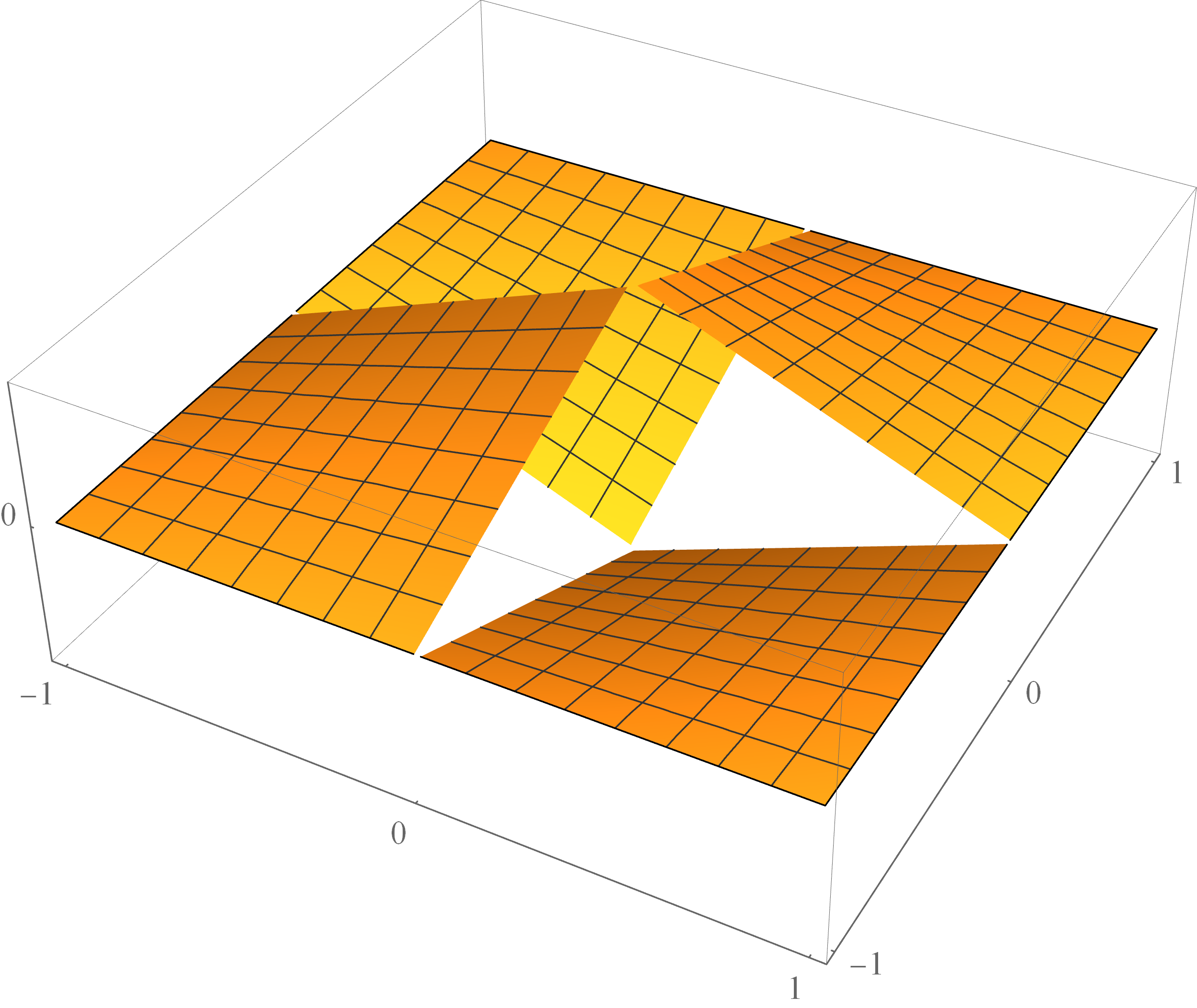
Figure 1: Midpoint rule $\phi$.

Proof.

It is simplest to first solve the normalized problem when $[a,b]\times[c,d]=[-1,1]\times[-1,1]$ and the function to be integrated is ${\tilde{f}}$. Define

$$\phi(s,t)=\left\{\begin{array}[]{lll}(s-1)(t-1);&0<s\leq 1,&0<t\leq 1\\ (s+1)(t-1);&-1\leq s<0,&0<t\leq 1\\ (s+1)(t+1);&-1\leq s<0,&-1\leq t<0\\ (s-1)(t+1);&0<s\leq 1,&-1\leq t<0.\end{array}\right.$$

See Figure 1 for a plot of $\phi$.

Consider integration in the region $[0,1]\times[0,1]$. Using Proposition 2.1,

$$\int_{0}^{1}\int_{0}^{1}{\tilde{f}}(s,t)\,dt\,ds={\tilde{f}}(0,0)-\int_{0}^{1}{\tilde{f}}_{s}(s,0)(s-1)\,ds$$

$$\qquad-\int_{0}^{1}{\tilde{f}}_{t}(0,t)(t-1)\,dt+\int_{0}^{1}\int_{0}^{1}{\tilde{f}}_{st}(s,t)(s-1)(t-1)\,dt\,ds.$$

There are similar formulas for the other three regions. We can then define $\gamma(x)=x+1$ for $x<0$ and $\gamma(x)=x-1$ for $x>0$. Next we have

$$\int_{-1}^{1}\int_{-1}^{1}{\tilde{f}}(s,t)\,dt\,ds=4{\tilde{f}}(0,0)-2\int_{-1}^{1}{\tilde{f}}_{s}(s,0)\gamma(s)\,ds$$

$$\qquad-2\int_{-1}^{1}{\tilde{f}}_{t}(0,t)\gamma(t)\,dt+\int_{-1}^{1}\int_{-1}^{1}{\tilde{f}}_{st}(s,t)\gamma(s)\gamma(t)\,dt\,ds.$$

This gives

$$\int_{-1}^{1}\int_{-1}^{1}{\tilde{f}}(s,t)\,dt\,ds=4{\tilde{f}}(0,0)+E({\tilde{f}}),$$ (12)

where

$$E({\tilde{f}}) = -2\int_{-1}^{1}{\tilde{f}}_{s}(s,0)\gamma(s)\,ds-2\int_{-1}^{1}{\tilde{f}}_{t}(0,t)\gamma(t)\,dt$$

$$\quad+\int_{-1}^{1}\int_{-1}^{1}{\tilde{f}}_{st}(s,t)\gamma(s)\gamma(t)\,dt\,ds.$$

Hölder’s inequality shows

$$\lvert E({\tilde{f}})\rvert\leq 2\lVert{\tilde{f}}_{s}(\cdot,0)\rVert_{p}\lVert\gamma\rVert_{q}+2\lVert{\tilde{f}}_{t}(0,\cdot)\rVert_{p}\lVert\gamma\rVert_{q}+\lVert{\tilde{f}}_{st}\rVert_{p}\lVert\gamma\rVert_{q}^{2},$$ (13)

where the norms are now taken over $[-1,1]$ and $[-1,1]\times[-1,1]$.

Note that if $1\leq q<\infty$, then

$$\lVert\gamma\rVert_{q}=\left(\int_{-1}^{0}(1+s)^{q}ds+\!\int_{0}^{1}(1-s)^{q}ds\right)^{1/q}\!\!\!=\left(2\!\int_{0}^{1}u^{q}du\right)^{1/q}\!\!\!=\left(\frac{2}{q+1}\right)^{1/q},$$

and, $\lVert\gamma\rVert_{\infty}=1$.

The transformation $x=(b-a)s/2+m_{1}$ and $y=(d-c)t/2+m_{2}$, maps the unit square onto $[a,b]\times[c,d]$. Let ${\tilde{f}}(s,t)=f(x,y)$. In (12),

$$\int_{-1}^{1}\int_{-1}^{1}{\tilde{f}}(s,t)\,dt\,ds=\frac{4}{(b-a)(d-c)}\int_{a}^{b}\int_{c}^{d}f(x,y)\,dy\,dx.$$ (14)

For $1\leq p<\infty$, we also have

$$\lVert{\tilde{f}}_{s}(\cdot,0)\rVert_{p} = \left(\int_{-1}^{1}\lvert{\tilde{f}}_{s}(s,0)\rvert^{p}\,ds\right)^{1/p}=\left(\int_{a}^{b}\left|\frac{\partial f(x,m_{2})}{\partial x}\frac{dx}{ds}\right|^{p}\,\frac{ds}{dx}\,dx\right)^{1/p}$$ (15)

$$= \lVert f_{x}(\cdot,m_{2})\rVert_{p}\left(\frac{dx}{ds}\right)^{1-1/p}=\lVert f_{x}(\cdot,m_{2})\rVert_{p}\left(\frac{b-a}{2}\right)^{1-1/p}.$$

And,

$$\lVert{\tilde{f}}_{s}(\cdot,0)\rVert_{\infty}=\max_{\lvert s\rvert\leq 1}\left|{\tilde{f}}_{s}(s,0)\right|=\max_{a\leq x\leq b}\left|f_{x}(x,m_{2})\frac{dx}{ds}\right|=\lVert f_{x}(\cdot,m_{2})\rVert_{\infty}(b-a)/2.$$

The other norms in (13) are handled similarly.

Now putting (15) and these other results into (14) and (13) gives the formulas in the theorem. ∎

Corollary 4.2 (Midpoint Composite Rule).

Define a uniform partition of $[a,b]$ by $x_{i}=a+i\Delta x$ where $\Delta x=(b-a)/m$ for some $m\in{\mathbb{N}}$. Then, for $0\leq i\leq m$, we have $a=x_{0}<x_{1}<\ldots<x_{m}=b$. Define a uniform partition of $[c,d]$ by $y_{j}=c+j\Delta y$ where $\Delta y=(d-c)/n$ for some $n\in{\mathbb{N}}$. Then, for $0\leq j\leq n$, we have $c=x_{0}<y_{1}<\ldots<y_{n}=d$. Let $m_{i}$ be the midpoint of $[x_{i-1},x_{i}]$, and $n_{j}$ be the midpoint of $[y_{j-1},y_{j}]$. We write

$$\int_{a}^{b}\int_{c}^{d}f(x,y)\,dy\,dx=\sum_{i=1}^{m}\sum_{j=1}^{n}f(m_{i},n_{j})\frac{(b-a)(d-c)}{mn}+E(f).$$

If $p=1$, then

$$\lvert E(f)\rvert \leq \sum_{j=1}^{n}\lVert f_{x}(\cdot,n_{j})\rVert_{1}\frac{(b-a)(d-c)}{2n}+\sum_{i=1}^{m}\lVert f_{y}(m_{i},\cdot)\rVert_{1}\frac{(b-a)(d-c)}{2m}$$

$$\quad+\frac{\lVert f_{xy}\rVert_{1}(b-a)(d-c)}{4}.$$

If $1<p<\infty$, then

$$\lvert E(f)\rvert \leq \sum_{j=1}^{n}\lVert f_{x}(\cdot,n_{j})\rVert_{p}\frac{(b-a)^{2-1/p}(d-c)}{2m^{1-1/p}n}+\sum_{i=1}^{m}\lVert f_{y}(m_{i},\cdot)\rVert_{p}\frac{(b-a)(d-c)^{2-1/p}}{2mn^{1-1/p}}$$

$$\quad+\frac{\lVert f_{xy}\rVert_{p}(b-a)^{2-1/p}(d-c)^{2-1/p}}{4(mn)^{1-1/p}}\left(\frac{p-1}{2p-1}\right)^{2(1-1/p)}.$$

If $p=\infty$, then

$$\lvert E(f)\rvert \leq \sum_{j=1}^{n}\lVert f_{x}(\cdot,n_{j})\rVert_{\infty}\frac{(b-a)^{2}(d-c)}{4mn}+\sum_{i=1}^{m}\lVert f_{y}(m_{i},\cdot)\rVert_{\infty}\frac{(b-a)(d-c)^{2}}{4mn}$$

$$\quad+\frac{\lVert f_{xy}\rVert_{\infty}(b-a)^{2}(d-c)^{2}}{4mn}.$$

If $\lvert\nabla f\rvert\leq M$ and $\lvert f_{xy}\rvert\leq N$ for some $M,N\in{\mathbb{R}}$, then

$$\lvert E(f)\rvert \leq \frac{M(b-a)^{2}(d-c)}{4m}+\frac{M(b-a)(d-c)^{2}}{4n}+\frac{N(b-a)^{2}(d-c)^{2}}{4mn}.$$

Proof.

Define

$$\phi(x,y)=\left\{\begin{array}[]{cl}(x-x_{i})(y-y_{j}),&(x,y)\in(m_{i},x_{i})\times(n_{j},y_{j})\\ (x-x_{i-1})(y-y_{j}),&(x,y)\in(x_{i-1},m_{i})\times(n_{j},y_{j})\\ (x-x_{i-1})(y-y_{j-1}),&(x,y)\in(x_{i-1},m_{i})\times(y_{j-1},n_{j})\\ (x-x_{i})(y-y_{j-1}),&(x,y)\in(m_{i},x_{i})\times(y_{j-1},n_{j}),\end{array}\right.$$

where

$$\gamma_{i}(x)=\left\{\begin{array}[]{cl}x-x_{i},&\text{ if }x\in(m_{i},x_{i})\text{ for some }1\leq i\leq m\\ x-x_{i-1},&\text{ if }x\in(x_{i-1},m_{i})\text{ for some }1\leq i\leq m\\ 0,&\text{ otherwise,}\end{array}\right.$$

$$\delta_{j}(y)=\left\{\begin{array}[]{cl}y-y_{j},&\text{ if }y\in(n_{j},y_{y})\text{ for some }1\leq j\leq n\\ y-y_{j-1},&\text{ if }y\in(y_{j-1},n_{j})\text{ for some }1\leq j\leq n\\ 0,&\text{ otherwise.}\end{array}\right.$$

Applying Proposition 2.1 to each of the four regions gives

$$\int_{x_{i-1}}^{x_{i}}\int_{y_{j-1}}^{y_{j}}f(x,y)\,dy\,dx\!\!\! =\!\!\! \frac{f(x_{i},y_{j})(b-a)(d-c)}{mn}$$ (19)

$$\quad-\frac{d-c}{n}\int_{x_{i-1}}^{x_{i}}f_{x}(x,n_{j})\gamma_{i}(x)\,dx$$

$$\quad-\frac{b-a}{m}\int_{y_{j-1}}^{y_{y}}f_{y}(m_{i},y)\delta_{j}(y)\,dy$$

$$\quad+\!\int_{x_{i-1}}^{x_{i}}\int_{y_{j-1}}^{y_{j}}f_{xy}(x,y)\gamma_{i}(x)\delta_{j}(y)\,dy\,dx.$$

Summing over $i$ and $j$, (19) gives the integral approximation.

Let $\chi_{I}$ be the characteristic function of interval $I$, that is $\chi_{I}(x)=1$ if $x\in I$ and $0$ otherwise.

From (19), with Hölder’s inequality,

$$\frac{d-c}{n}\left|\sum_{i=1}^{m}\sum_{j=1}^{n}\int_{x_{i-1}}^{x_{i}}f_{x}(x,n_{j})\gamma_{i}(x)\,dx\right|$$

$$\qquad\leq\frac{d-c}{n}\sum_{j=1}^{n}\int_{a}^{b}\lvert f_{x}(x,n_{j})\gamma_{i}(x)\chi_{(x_{i-1},x_{i})}(x)\rvert\,dx$$

$$\qquad\leq\frac{d-c}{n}\sum_{j=1}^{n}\lVert f_{x}(\cdot,n_{j})\rVert_{p}\lVert\gamma_{i}(x)\chi_{(x_{i-1},x_{i})}\rVert_{q}.$$

Note that

$$\lVert\gamma_{i}(x)\chi_{(x_{i-1},x_{i})}\rVert_{q} = \left(\sum_{i=1}^{m}\int_{x_{i-1}}^{m_{i}}\lvert x-x_{i-1}\rvert^{q}\,dx+\int_{m_{i}}^{x_{i}}\lvert x-x_{i}\rvert^{q}\,dx\right)^{1/q}$$

$$= \left(2\sum_{i=1}^{m}\int_{0}^{\Delta x/2}x^{q}\,dx\right)^{1/q}$$

$$= \left\{\begin{array}[]{cl}\frac{b-a}{2},&p=1\\ \frac{(b-a)^{2-1/p}}{2m^{1-1/p}}\left(\frac{p-1}{2p-1}\right)^{1-1/p},&1<p<\infty\\ \frac{(b-a)^{2}}{4m},&p=\infty.\end{array}\right.$$

Equation (19) is handled similarly.

With (19) we let $\Gamma(x,y)=\gamma_{i}(x)\delta_{j}(y)$ if $(x,y)\in(x_{i-1},x_{i})\times(y_{j-1},y_{j})$ for some $i$ and $j$, and $\Gamma$ is zero otherwise. Then

$$\left|\sum_{i=1}^{m}\sum_{j=1}^{n}\int_{x_{i-1}}^{x_{i}}\int_{y_{j-1}}^{y_{j}}f_{xy}(x,y)\gamma_{i}(x)\delta_{j}(y)\,dy\,dx\right| \leq \int_{a}^{b}\lvert f_{xy}(x,y)\Gamma(x,y)\rvert\,dy\,dx$$

$$\leq \lVert f_{xy}\rVert_{p}\lVert\Gamma\rVert_{q},$$

and

$$\lVert\Gamma\rVert_{q} = \left(\sum_{i=1}^{m}\sum_{j=1}^{n}\int_{x_{i-1}}^{x_{i}}\lvert\gamma_{i}(x)\rvert^{q}\,dx\int_{y_{j-1}}^{y_{j}}\lvert\delta_{j}(y)\rvert^{q}\,dy\right)^{1/q}$$

$$= \left(4\sum_{i=1}^{m}\sum_{j=1}^{n}\int_{0}^{\Delta x/2}x^{q}\,dx\int_{0}^{\Delta y/2}y^{q}\,dy\right)^{1/q}$$

$$= \left\{\begin{array}[]{cl}\frac{(b-a)(d-c)}{4},&p=1\\ \frac{(b-a)^{2-1/p}(d-c)^{2-1/p}}{4(mn)^{1-1/p}}\left(\frac{p-1}{2p-1}\right)^{2(1-1/p)},&1<p<\infty\\ \frac{(b-a)^{2}(d-c)^{2}}{4mn},&p=\infty.\end{array}\right.$$

∎

Remark.

At the end of Corollaries 3.3 and 4.2 we have estimates for the error in the trapezoidal and midpoint composite rules under the assumptions $\lvert\nabla f\rvert\leq M$ and $\lvert f_{xy}\rvert\leq N$ for some $M,N\in{\mathbb{R}}$. If we take partitions with equal number of intervals in the $x$ and $y$ direction ($m=n$) then the error estimates for both composite rules are $E(f)=O(1/n)$ as $n\to\infty$.

Note that only under the assumptions that $\lVert f_{x}(\cdot,y)\rVert_{p}$ is uniformly bounded for $c\leq y\leq d$ and $\lVert f_{y}(x,\cdot)\rVert_{p}$ is uniformly bounded for $a\leq x\leq b$ the trapezoidal rule has a better error estimate ($E(f)=O(1/n)$) than the midpoint rule ($E(f)=O(1/n^{1-1/p})$).

5 Minimizing error estimates

The error estimate in Proposition 2.2 depends on $\lVert\phi\rVert_{q}$, where $\phi(x,y)=xy+\alpha(x)+\beta(y)$. We needed to choose particular functions $\alpha$ and $\beta$ to generate the trapezoidal rule (Theorem 3.1) and the midpoint rule (Theorem 4.1). A natural question is: how can $\alpha$ and $\beta$ be chosen to minimize $\lVert\phi\rVert_{q}$? As we see below, if $1<q<\infty$, there is a unique function of this type that minimizes the norm of $\phi$ and this is the same $\phi$ as in the trapezoidal rule of Theorem 3.1. If $q=\infty$ the minimizer is not unique but the minimum norm is the same as in the trapezoidal rule. For $q=1$ we find the minimum norm but know nothing about uniqueness of the minimizing function.

First note that in a normed linear space $X$ with norm $\lVert\cdot\rVert$, if $x_{i}\in X$ are linearly independent and $z\in X$, then the problem of finding $a_{i}\in{\mathbb{R}}$ to minimize $\lVert z-a_{1}x_{1}-a_{2}x_{2}-\cdots-a_{n}x_{n}\rVert$ has a solution for each $n\in{\mathbb{N}}$. This is called the problem of best approximation. For example, [4, Theorem 7.4.1]. Whether this problem has a unique solution depends on the notion of a strictly convex normed linear space: $X$ is strictly convex if for all $x,y\in X$ with $\lVert x\rVert=\lVert y\rVert=1$ and $x\not=y$ we have $\lVert(x+y)/2\rVert<1$. Geometrically, this means the surface of a ball contains no line segments. It is known that for $1<p<\infty$ the spaces $L^{p}([-1,1]\times[-1,1])$ are strictly convex and are not strictly convex if $p=1$ or if $p=\infty$. See [8, p. 112, exercise 3]. If the elements $x_{i}$ are linearly independent in $X$, and $X$ is strictly convex, then the best approximation problem has a unique solution [4, Theorem 7.5.3].

Theorem 5.1.

Define $\phi\!:\![a,b]\times[c,d]\to{\mathbb{R}}$ by $\phi(x,y)=xy+\alpha(x)+\beta(y)$ where $\alpha$ and $\beta$ are functions of one variable in $L^{q}([-1,1])$. The minimum of $\lVert\phi\rVert_{q}$, by varying $\alpha$ and $\beta$, is

$$\lVert\phi\rVert_{q}=\left\{\begin{array}[]{cl}\left(\frac{2}{q+1}\right)^{2/q},&1<q<\infty\\ 1,&q=1\text{ or }\infty.\end{array}\right.$$

If $1<q<\infty$, then the unique minimum is given by $\phi(x,y)=(x-m_{1})(y-m_{2})$ where $m_{1}$ is the midpoint of $[a,b]$, and $m_{2}$ is the midpoint of $[c,d]$. If $q=1$, or $q=\infty$, the minimum is achieved by more than one function, but $\lVert\phi\rVert_{\infty}=1$ with $\phi(x,y)=(x-m_{1})(y-m_{2})$.

Proof.

It suffices to consider $[a,b]\times[c,d]=[-1,1]\times[-1,1]$, and then a linear transformation can be used to map the unit square onto $[a,b]\times[c,d]$.

Let $\psi(x,y)=xy$.

If $1<q<\infty$ then the $q$-norm is strictly convex. By the paragraph preceding the theorem, this means that if $x_{i}$ are fixed linearly independent functions in $L^{q}([-1,1]^{2})$, then for each $n\in{\mathbb{N}}$ the problem of choosing $a_{i}\in{\mathbb{R}}$ to minimize $\lVert\psi+a_{1}x_{1}+\ldots+a_{n}x_{n}\rVert_{q}$ has a unique solution. In our problem, the functions $x_{i}$ are functions of one variable. We first need a result on linear independence.

Suppose $\alpha_{e}$, $\alpha_{o}$, $\beta_{e}$, and $\beta_{o}$ are, respectively, non-constant even and odd functions of one variable. We claim that the set of functions $\{\alpha_{e}(s),\alpha_{o}(s),\beta_{e}(t),\\ \beta_{o}(t)\}$ is linearly independent on $[-1,1]^{2}$. Suppose $\lambda_{1}\alpha_{e}(s)+\lambda_{2}\alpha_{o}(s)+\lambda_{3}\beta_{e}(t)+\lambda_{4}\beta_{o}(t)=0$ for all $(s,t)\in[-1,1]^{2}$ for some constants $\lambda_{i}$. Then $\lambda_{1}\alpha_{e}(s)+\lambda_{2}\alpha_{o}(s)=-\lambda_{3}\beta_{e}(t)-\lambda_{4}\beta_{o}(t)$. Since $s$ and $t$ can be varied independently this shows existence of a constant $k$ so that $\lambda_{1}\alpha_{e}(s)+\lambda_{2}\alpha_{o}(s)=-\lambda_{3}\beta_{e}(t)-\lambda_{4}\beta_{o}(t)=k$ for all $s$ and $t$. Let $s\not=0$. Then $\lambda_{1}\alpha_{e}(s)-\lambda_{2}\alpha_{o}(s)=k$. Adding gives $\lambda_{1}\alpha_{e}(s)=k$. Since $\alpha_{e}$ is not constant we must have $\lambda_{1}=k=0$. Subtracting the equations now gives $\lambda_{2}\alpha_{o}(s)=0$ and $\alpha_{2}$ is not constant so $\lambda_{2}=0$. Similarly, $\lambda_{3}=\lambda_{4}=0$ and the functions are linearly independent.

With the functions $\alpha_{e}$, $\alpha_{o}$, $\beta_{e}$ and $\beta_{o}$ fixed as above consider the expression

$$\lVert\psi+a_{1}\alpha_{e}+a_{2}\alpha_{o}+a_{3}\beta_{e}+a_{4}\beta_{o}\rVert_{q}^{q}$$

$$\quad=\int_{-1}^{1}\int_{-1}^{1}\lvert st+a_{1}\alpha_{e}(s)+a_{2}\alpha_{o}(s)+a_{3}\beta_{e}(t)+a_{4}\beta_{o}(t)\rvert^{q}\,dt\,ds,$$

where $a_{1}$, $a_{2}$, $a_{3}$, $a_{4}$ are the unique constants that give the minimum. Changing variables $(s,t)\mapsto(-s,t)$ in the integral gives

$$\lVert\psi+a_{1}\alpha_{e}+a_{2}\alpha_{o}+a_{3}\beta_{e}+a_{4}\beta_{o}\rVert_{q}^{q}=\lVert\psi-a_{1}\alpha_{e}+a_{2}\alpha_{o}-a_{3}\beta_{e}-a_{4}\beta_{o}\rVert_{q}^{q}.$$

But the coefficients are unique so $a_{1}=-a_{1}$, $a_{3}=-a_{3}$ and $a_{4}=-a_{4}$. Hence, these coefficients are $0$. The change of variables $(s,t)\mapsto(s,-t)$ in the integral now shows $a_{2}=0$. Therefore, for any set of fixed even and odd functions of one variable the minimum of $\lVert\psi+a_{1}\alpha_{e}+a_{2}\alpha_{o}+a_{3}\beta_{e}+a_{4}\beta_{o}\rVert_{q}$ is $\lVert\psi\rVert_{q}$.

Now we show that we get the same result when we vary the functions. Suppose $\alpha$ and $\beta$ are any fixed functions in $L^{q}([-1,1])$. The even part of $\alpha$ is $\alpha_{e}(s)=(\alpha(s)+\alpha(-s))/2$ and the odd part is $\alpha_{o}(s)=(\alpha(s)-\alpha(-s))/2$. Similarly with $\beta$. Again, using the convention that $\alpha$ functions are evaluated at the first variable and $\beta$ functions at the second variable, we have

$$\min_{c_{1},c_{2}\in{\mathbb{R}}}\lVert\psi+c_{1}\alpha+c_{2}\beta\rVert_{q} = \min_{c_{1},c_{2}\in{\mathbb{R}}}\lVert\psi+c_{1}\alpha_{e}+c_{1}\alpha_{o}+c_{2}\beta_{e}+c_{2}\beta_{o}\rVert_{q}$$

$$\geq \min_{a_{i}\in{\mathbb{R}}}\lVert\psi+a_{1}\alpha_{e}+a_{2}\alpha_{o}+a_{3}\beta_{e}+a_{4}\beta_{o}\rVert_{q}=\lVert\psi\rVert_{q}.$$

But taking $c_{1}=c_{2}=0$ gives $\lVert\psi\rVert_{q}$ in $\lVert\psi+c_{1}\alpha+c_{2}\beta\rVert_{q}$ so this is its minimum as well.

Suppose there were functions $\xi,\eta\in L^{q}([-1,1])$ so that if $\xi$ is evaluated at the first variable and $\eta$ is evaluated at the second variable then $\lVert\psi+\xi+\eta\rVert_{q}<\lVert\psi\rVert_{q}$. Then

$$\lVert\psi+\xi+\eta\rVert_{q}=\lVert\psi+1\xi+1\eta\rVert_{q}\geq\min_{c_{1},c_{2}\in{\mathbb{R}}}\lVert\psi+c_{1}\xi+c_{2}\eta\rVert_{q}=\lVert\psi\rVert_{q}.$$

This contradiction shows that

$$\min_{\alpha,\beta\in L^{q}([-1,1])}\lVert\psi+\alpha+\beta\rVert_{q}=\lVert\psi\rVert_{q}.$$

The norm is computed following (13).

Now consider $q=\infty$. The maximum of $\psi(x,y)=xy$ on $[-1,1]\times[-1,1]$ is $\psi(1,1)=\psi(-1,-1)=1$ and the minimum is $\psi(1,-1)=\psi(-1,1)=-1$. Hence, $\lVert\psi\rVert_{\infty}=1$. For $\phi(s,t)=st+\alpha(s)+\beta(t)$ to have $\lVert\phi\rVert_{\infty}\leq\lVert\psi\rVert_{\infty}$, we must have

$$\alpha(1)+\beta(1) \leq 0,$$ (22)

$$\alpha(-1)+\beta(-1) \leq 0,$$ (23)

$$\alpha(1)+\beta(-1) \geq 0,$$ (24)

$$\alpha(-1)+\beta(1) \geq 0.$$ (25)

This is because the maximum of $\psi$ is positive, and the minimum is negative. And,

$$\eqref{ab1}\text{ and }\eqref{ab3} \beta(1)-\beta(-1)\leq 0,$$ give

$$\eqref{ab2}\text{ and }\eqref{ab4} \beta(-1)-\beta(1)\leq 0;$$ give

hence $\beta(1)=\beta(-1)$. Similarly, $\alpha(1)=\alpha(-1)$. Equations (22) and (24) now show $0\leq\alpha(1)+\beta(1)\leq 0$ and so $\alpha(1)+\beta(1)=0$. We then get $\alpha(1)=\alpha(-1)=-\beta(1)=-\beta(-1)$. But then

$$\phi(1,1) = 1+\alpha(1)+\beta(1)=1$$

$$\phi(-1,-1) = 1+\alpha(-1)+\beta(-1)=1$$

$$\phi(1,-1) = -1+\alpha(1)+\beta(-1)=-1$$

$$\phi(-1,1) = -1+\alpha(-1)+\beta(1)=-1.$$

This shows $\lVert\phi\rVert_{\infty}\geq 1=\lVert\psi\rVert_{\infty}$, so $\min_{\alpha,\beta}\lVert\phi\rVert_{\infty}=\lVert\psi\rVert_{\infty}=1$.

Now consider $q=1$. Given $\epsilon>0$, for each $\alpha,\beta\in L^{1}([-1,1])$, there are continuous functions ${\overline{\alpha}},{\overline{\beta}}$ such that $\lvert\lVert\psi+\alpha+\beta\rVert_{1}-\lVert\psi+{\overline{\alpha}}+{\overline{\beta}}\rVert_{1}\rvert<\epsilon$. Then ${\overline{\alpha}},{\overline{\beta}}\in L^{q}([-1,1])$ for each $1\leq q\leq\infty$ so

$$\lVert\psi+\alpha+\beta\rVert_{1} \geq \lVert\psi+{\overline{\alpha}}+{\overline{\beta}}\rVert_{1}-\epsilon$$

$$= \lim_{q\to 1^{+}}\lVert\psi+{\overline{\alpha}}+{\overline{\beta}}\rVert_{q}-\epsilon$$

$$\geq \lim_{q\to 1^{+}}\lVert\psi\rVert_{q}-\epsilon$$

$$= \lim_{q\to 1^{+}}\left(\int_{-1}^{1}\int_{-1}^{1}\lvert st\rvert^{q}\,dt\,ds\right)^{1/q}-\epsilon$$

$$= \lim_{q\to 1^{+}}\left(2\int_{0}^{1}s^{q}\,ds\right)^{2/q}-\epsilon$$

$$= \lim_{q\to 1^{+}}\left(\frac{2}{q+1}\right)^{2/q}-\epsilon$$

$$= 1-\epsilon.$$

Therefore, since $\epsilon>0$ is arbitrary,

$$\min_{\alpha,\beta\in L^{1}([-1,1])}\lVert\psi+\alpha+\beta\rVert_{1}\geq 1.$$

But,

$$\lVert\psi+0\alpha+0\beta\rVert_{1}=\int_{-1}^{1}\int_{-1}^{1}\lvert st\rvert\,dt\,ds=4\left(\int_{0}^{1}s\,ds\right)^{2}=1.$$

Hence,

$$\min_{\alpha,\beta\in L^{1}([-1,1])}\lVert\psi+\alpha+\beta\rVert_{1}=1.$$

An example that shows the minimizing function is not unique when $q=\infty$ is $\phi(s,t)=st-\lvert s\rvert+\lvert t\rvert$. The gradient does not vanish in any of the four open regions $(0,1)\times(0,1)$, $(-1,0)\times(0,1)$, $(-1,0)\times(-1,0)$ or $(0,1)\times(-1,0)$. The extreme values are then on the $s$-axis for $\lvert s\rvert\leq 1$, on the $t$-axis for $\lvert t\rvert\leq 1$, on one of the line segments given by $\lvert s\rvert=1$, or on one of the line segments given by $\lvert t\rvert=1$. It is then seen that the maxima and minima on these line segments are $1$ and $-1$. Hence, $\lVert\phi\rVert_{\infty}=1$. Further examples with unit norm can be obtained by considering $\phi(s,t)=st\pm u\lvert s\rvert^{v}\mp u\lvert t\rvert^{v}$ for $u,v>0$. A linear transformation then maps the unit square onto $[a,b]\times[c,d]$. ∎

We do not know of an example of non-uniqueness of the minimizing function when $q=1$.

An approach to the proof for $q=2$ that does not require facts about the uniform convexity of the norm is the following. Note that

$$\int_{-1}^{1}\int_{-1}^{1}\lvert st+\alpha(s)+\beta(t)\rvert^{2}\,dt\,ds$$

$$\qquad=\int_{-1}^{1}\int_{-1}^{1}\left\{s^{2}t^{2}+2st\alpha(s)+2st\beta(t)+[\alpha(s)+\beta(t)]^{2}\right\}\,dt\,ds$$

$$\qquad=\int_{-1}^{1}\int_{-1}^{1}\left\{s^{2}t^{2}+[\alpha(s)+\beta(t)]^{2}\right\}\,dt\,ds.$$

The norm of $\phi$ is then minimized when $\alpha(s)=-\beta(t)$. Then $\alpha$ and $\beta$ are both constant so the minimizer is $\phi(s,t)=st$.

6 Acknowledgments

The first author was partially funded by a work/study grant from the University of the Fraser Valley.

References

- [1] J.J. Benedetto and W. Czaja, Integration and modern analysis, Boston, Birkhäuser, 2009.
- [2] D. Cruz-Uribe and C.J. Neugebauer, Sharp error bounds for the trapezoidal rule and Simpson’s rule, JIPAM. J. Inequal. Pure Appl. Math. 3(2002), Article 49, 22 pp.
- [3] A.E. Currier, Proof of the fundamental theorems on second-order cross partial derivatives, Trans. Amer. Math. Soc. 35(1933), 245–253.
- [4] P.J. Davis, Interpolation and approximation, New York, Dover, 1975.
- [5] S. Haber, Numerical evaluation of multiple integrals, SIAM Rev. 12(1970), 481–526.
- [6] R.M. McLeod, The generalized Riemann integral, Washington, Mathematical Association of America, 1980.
- [7] Sh. E. Mikeladze, Numerical methods of mathematical analysis, Moscow, State Publishing House of Technical-Theoretical Literature, 1953.
- [8] W. Rudin, Real and complex analysis, New York, McGraw-Hill, 1987.
- [9] A. Sard, Linear approximation, Providence, Rhode Island, American Mathematical Society, 1963.
- [10] A.H. Stroud, Approximate calculation of multiple integrals, Englewood Cliffs, New Jersey, Prentice-Hall, 1971.
- [11] E. Talvila and M. Wiersma, Simple derivation of basic quadrature formulas, Atl. Electron. J. Math. 5(2012), 47–59.
- [12] C.W. Ueberhuber, Numerical computation, vol. II, Berlin, Springer–Verlag, 1997.