A measurement of the cosmic microwave background lensing potential and power spectrum from 500 deg² of SPTpol temperature and polarization data

Abstract

We present a measurement of the cosmic microwave background (CMB) lensing potential using 500 deg² of 150 GHz data from the SPTpol receiver on the South Pole Telescope. The lensing potential is reconstructed with signal-to-noise per mode greater than unity at lensing multipoles $L\lesssim 250$, using a quadratic estimator on a combination of CMB temperature and polarization maps. We report measurements of the lensing potential power spectrum in the multipole range of $100<L<2000$ from sets of temperature-only (T), polarization-only (POL), and minimum-variance (MV) estimators. We measure the lensing amplitude by taking the ratio of the measured spectrum to the expected spectrum from the best-fit $\Lambda$CDM model to the Planck 2015 TT+lowP+lensing dataset. For the minimum-variance estimator, we find $A_{\rm{MV}}=0.944\pm 0.058{\rm\,(Stat.)}\pm 0.025{\rm\,(Sys.)}$; restricting to only polarization data, we find $A_{\rm{POL}}=0.906\pm 0.090{\rm\,(Stat.)}\pm 0.040{\rm\,(Sys.)}$. Considering statistical uncertainties alone, this is the most precise polarization-only lensing amplitude constraint to date ($10.1\,\sigma$), and is more precise than our temperature-only constraint. We perform null tests and consistency checks and find no evidence for significant contamination.

1. Introduction

Gravitational potentials associated with large-scale structure deflect the paths of cosmic microwave background (CMB) photons as they propagate from the surface of last scattering – a process called gravitational lensing (Blanchard & Schneider, 1987). Gravitational lensing breaks the statistical isotropy of the CMB and introduces correlations across CMB temperature and polarization fluctuations on different angular scales. These correlations are proportional to the projected gravitational potentials integrated along the line of sight and therefore can be used to reconstruct the lensing potential (Lewis & Challinor, 2006). The lensing potential is a probe of the growth of large-scale structure and the geometry of the universe between the epoch of recombination and today. Thus, from CMB observations alone, we can extract information about the universe at both the redshift of last scattering ($z\simeq 1100$) and the redshifts of structure formation ($z\lesssim 3$) and dark energy domination. This makes CMB lensing a powerful tool for pursuing some of the most ambitious goals in cosmology and particle physics today (e.g. CMB-S4 Collaboration et al., 2016), including constraining the sum of neutrino masses and the amplitude of primordial gravitational waves (Lesgourgues & Pastor, 2006; Kamionkowski & Kovetz, 2016).

While using the CMB lensing measurements from this work, we will not detect the sum of neutrino masses or significantly constrain primordial gravitational waves through delensing (Manzotti et al., 2017), these measurements will nevertheless provide relevant constraints to parameters of the standard cosmological model $\Lambda$CDM. This is of particular interest currently because some optical probes of gravitational lensing are in mild tension with Planck’s CMB+lensing constraints on matter density and fluctuations (Abbott et al., 2018a; Hildebrandt et al., 2018; Hikage et al., 2019). The optical lensing measurements use the effect of gravitational lensing on the apparent shapes of background galaxies to measure the intervening gravitational potentials. Compared with using galaxies, an attractive characteristic of CMB lensing is that the source plane has nearly Gaussian statistics with a well-characterized angular power spectrum and is at a high and well-known redshift $z=1089.8\pm 0.2$ (Planck Collaboration et al., 2016a, 2018a). Owing to the high-redshift source plane, CMB lensing probes the integrated matter fluctuations to redshifts beyond optical surveys. Furthermore, CMB lensing measurements have different instrumental and astrophysical systematics compared with those from optical surveys. The use of independent probes will therefore help us investigate the source of the tension. It is thus an important goal for us to identify potential sources of instrumental and/or astrophysical systematics as the field advances the precision of CMB lensing measurements.

In the last few years, CMB lensing has entered the era of precision measurements. This lensing effect was first detected through cross correlations with radio sources (Smith et al., 2007). Since then, the CMB lensing potential power spectrum has been measured by multiple groups using temperature data only (T, Das et al. 2011; van Engelen et al. 2012; Planck Collaboration XVII 2013; Omori et al. 2017), polarization data only (POL, POLARBEAR Collaboration 2014; Keck Array et al. 2016), and combinations of temperature and polarization data (Story et al., 2015; Sherwin et al., 2017; Planck Collaboration et al., 2018b). The most precise lensing amplitude measurement, at 40 $\sigma$, comes from Planck’s minimum-variance (MV) estimator that combines both temperature and polarization estimators; in that measurement, the temperature reconstruction contributes most of the signal-to-noise ratio (S/N). More generally, in prior lensing measurements that used both temperature and polarization maps, the T estimator has always dominated the overall measurement precision. In this work, for the first time, the POL measurement is more constraining than the T measurement. Furthermore, if we consider only the statistical uncertainty, we have a $10\%$ constraint ($10.1\,\sigma$) on the lensing amplitude using polarization data alone – the tightest constraint of its kind to date.

In this work, we extend the lensing measurement to a 500 deg² field from the 100 deg² field of Story et al. (2015, hereafter S15). We build on the lensing pipeline presented in S15 with two main modifications. First, instead of including the Monte Carlo (MC) bias – the difference between the recovered lensing spectrum from simulation and the input spectrum – as a systematic uncertainty, we identify its main contributor and correct for the bias using a multiplicative correction factor. Second, instead of treating extragalactic foreground biases as negligible, we subtract an expected foreground bias from the T and MV lensing spectra.

Because the input CMB maps are of similar depths as those used in S15, we also measure lensing modes with S/N better than unity for $L\lesssim 250$. However, in this analysis, we have $\sim$5 times more sky area and therefore are able to make a more precise measurement of the lensing spectrum. With both the T and POL lensing amplitudes well constrained, we improve the precision of the MV lensing amplitude measurement from S15’s 14% to $6\%$. This is approaching the $\sim$3% precision of the lensing amplitude measurement from Planck (Planck Collaboration et al., 2018b). These two measurements arrive at their respective precisions from very different regimes: while the Planck measurement covers 67% of the sky, each lensing mode is measured with low S/N; our measurement covers only 1% of the sky, but many lensing modes are measured with high S/N. When our measurements are projected to cosmological parameter space, the constraint in the $\sigma_{8}-\Omega_{M}$ plane is only slightly weaker than those from Planck (Planck Collaboration et al., 2018b). This will be useful in illuminating the aforementioned mild tension between optical probes and Planck. In a future paper, we will present cosmological parameter constraints and comparisons with other lensing probes.

This paper is organized as follows: in Section 2, we describe the dataset used and the simulated skies generated for this analysis. In Section 3, we summarize the lensing analysis pipeline and describe new aspects. We present the lensing measurements in Section 4 and show that our measurements are robust against systematics in Section 5.1. In Section 5.2, we account for systematic uncertainties from sources that can bias the lensing measurement. We conclude in Section 6.

2. Data and Simulations

In this section, we describe the SPTpol survey, the data processing steps taken to generate the data maps, and the simulated skies generated for this analysis.

2.1. SPTpol 500 deg² survey

The South Pole Telescope (SPT, Padin et al., 2008; Carlstrom et al., 2011) is a 10-meter diameter off-axis Gregorian telescope located at the Amundsen-Scott South Pole Station in Antarctica. In this work, we use data from the 150 GHz detectors from the first polarization-sensitive receiver on SPT, SPTpol. The SPTpol 500 deg² survey spans 4 hours in right ascension (R.A.), from $22^{h}$ to $2^{h}$, and 15 degrees in declination (dec.), from $-65\deg$ to $-50\deg$. We use observations conducted between April 30, 2013 and October 27, 2015 (after the 100 deg² survey for S15 was finished), which include 3491 independent maps of the 500 deg² survey footprint. The field was observed using two strategies. Initially, we used a “lead-trail” scanning strategy, where the field was divided into two halves in R.A.. The telescope first scanned the lead half, and then switched to the trail half such that they were both observed over the same range in azimuth, and therefore the same patch of ground. In May 2014, the scanning strategy was switched to a “full-field” strategy, in which the full R.A. range of the field was covered in a single observation.

2.2. Data processing

The data reduction for this set of maps follows that applied to the TE/EE power spectrum analysis of the same field (Henning et al., 2018, hereafter H18). We therefore highlight here only aspects that are different or are particularly relevant for this analysis.

An observation is built from a collection of constant-elevation scans, where the telescope moves from one end of the R.A. range to the other. For every scan, we filter the time streams, which corresponds in map space to mode removal along the scan direction. We subtract from each detector’s time stream a Legendre polynomial as an effective high-pass filter. We choose a 3rd order polynomial for the lead-trail scans and a 5th order polynomial for the full-field scans. We combine this with a high-pass filter with a cutoff frequency corresponding to angular multipole $\ell=100$ in the scan direction. During the polynomial and high-pass filtering step, regions within $5^{\prime}$ of point sources brighter than 50 mJy at 150 GHz are masked in the time streams to avoid ringing artifacts. Finally, we low-pass the time streams at an effective multipole of $\ell=7500$ in the scan direction to avoid high-frequency noise aliasing into the signal due to the adopted pixel resolution of $1^{\prime}$ in the maps.

Electrical cross talk between detectors can bias our measurement. In S15, we accounted for this bias as a systematic uncertainty of 5% on the MV lensing amplitude. In this analysis, we correct the cross talk between detectors at the time stream level as described in H18. With this correction, cross talk is suppressed by more than an order of magnitude. With the 5% uncertainty from S15 being an upper limit before this suppression, we conclude that the residual cross talk introduces negligible bias to our lensing amplitude measurement.

Before binning into maps, we calibrate the time streams relative to each other using observations of the HII region RCW38 and an internal chopped thermal source. The per-detector polarization angles are calibrated based on measurements from a polarized thermal source (Crites et al., 2015). After that, the time stream data are binned into $T/Q/U$ maps with $1^{\prime}\times 1^{\prime}$ pixels using the oblique Lambert azimuthal equal-area projection.

We apply the following corrections to the coadded map of the individual observations to obtain the final map: $T\rightarrow P$ monopole subtraction, global polarization rotation, absolute calibration, and source and boundary masking. We measure $T\rightarrow P$ leakage by taking a weighted average over multipole space of the cross correlation of the temperature map with either the $Q$ or the $U$ map. We find leakage factors of $\epsilon^{Q}=0.018$ and $\epsilon^{U}=0.008$. We obtain their uncertainties from the spread of leakage factors derived from 100 different half-splits of the data and find the fractional uncertainties to be 0.1% and 0.3% respectively. We deproject a monopole leakage term from the maps by subtracting a copy of the temperature map scaled by these factors from the $Q$ and $U$ maps.

Assuming $\Lambda$CDM cosmology, we expect the cross spectra $TB$ and $EB$ to be consistent with zero. Therefore, we can estimate and apply the global polarization angle rotation needed to minimize the $TB$ and $EB$ correlations (Keating et al., 2013). We find the rotation angle to be $0.63^{\circ}\pm 0.04^{\circ}$ and rotate the $Q$ and $U$ maps accordingly.

The final absolute calibration is obtained by comparing the final coadded SPTpol $T$ map with Planck  over the angular multipole range $600<\ell<1000$. Specifically, we take the ratio of the cross spectrum of two half-depth SPTpol maps to the cross spectrum of full-depth SPTpol and Planck maps and require the ratio to be consistent with 1 to determine the calibration factor. We estimate the polarization efficiency (or polarization calibration factor) similarly, by comparing a full-depth SPTpol $E$-mode map with the Planck $E$-mode map. The temperature and polarization calibration factors ($T_{\rm cal}$ and $P_{\rm cal}$) as derived are $0.9088$ and $1.06$ respectively (see H18 for details). We apply $T_{\rm cal}$ to the temperature map and $T_{\rm cal}\times P_{\rm cal}$ to the polarization maps to obtain calibrated temperature and polarization maps. In the legacy Planck release, their polarization efficiency estimates are found to be potentially biased at the $1-2\%$ level (see Table 9 of Planck Collaboration et al., 2018c). To circumvent potential biases when we tie our polarization map calibration to Planck’s $E$-mode map, we adjust $P_{\rm cal}$ by a multiplicative factor obtained from H18 without using Planck’s polarization maps. In H18, $T_{\rm cal}$ and $P_{\rm cal}$ were free parameters in the fits of the PlanckTT+SPTpol EETE dataset to the $\Lambda$CDM + foregrounds + nuisance parameters model, with priors set by the $T_{\rm cal}$ and $P_{\rm cal}$ values and uncertainties derived from the comparison against Planck described above. In this work, we multiply $P_{\rm cal}$ by the best-fit $P_{\rm cal}$ parameter (1.01) from H18 (see Table 5 of H18). In Section 5.2, we use the posterior uncertainties of the $T_{\rm cal}$ and $P_{\rm cal}$ parameters to quantify their contributions to the systematic uncertainties of the lensing amplitude measurements.

We apply a mask that defines the boundary of the $T/Q/U$ maps to downweight the noisy field edges. In addition, we mask bright point sources in the map. We use a $5^{\prime}$ radius to mask point sources from the SPT-SZ catalog by Everett et al. in prep. with flux density above 6 mJy at either 95 GHz or 150 GHz that are in the 500 deg² footprint. We use a $10^{\prime}$ radius for point sources with flux density greater than 90 mJy at either 95 GHz or 150 GHz. Clusters detected in Bleem et al. (2015) within the 500 deg² survey footprint are masked using a $10^{\prime}$ radius. The mask has a top hat profile for both the boundary and the sources, and mode mixing due to the mask is suppressed by the inverse-variance map-filtering step (Section 3.2). We compare this lensing measurement with one using a cosine-tapered apodization on the mask edges in Section 5.2 and find them to be consistent.

The noise levels in the coadded maps are 11.8 $\mu$K–arcmin in temperature and 8.3 $\mu$K–arcmin in polarization over the multipole range $1000<\ell<3000$. The map depth is similar to that of the 100 deg² field used in S15. Since this map covers five times the sky area, the sample variance of the lensing power spectrum is reduced and hence the lensing spectrum measurement precision is improved.

2.3. Simulations

We use simulated skies to estimate the mean-field bias $\bar{\phi}^{\rm MF}$ to the lensing potential map (Section 3.1), to correct the analytical response of the lensing estimator (Section 3.1), to correct the expected biases ($N_{L}^{(0),\rm RD}$and $N_{L}^{(1)}$, see Section 3.3) in the raw lensing power spectrum, and to estimate the uncertainties of the lensing measurements (Section 4).

The simulated skies contain the CMB, foregrounds, and instrumental noise. The input cosmology for generating the CMB is the best-fit $\Lambda$CDM model to the Planck plikHM_TT_lowTEB_lensing dataset (second column in Table 4 of Planck Collaboration et al., 2016b). Using the best-fit cosmology, we use CAMB to generate theory spectra, which are then fed into Healpix (Górski et al., 2005) to generate the spherical harmonic coefficients $a_{\ell m}$ for $T,E,B$, and the lensing potential $\phi$. The CMB $a_{\ell m}$ are projected to maps and lensed by $\phi$ using LensPix (Lewis, 2005). The lensed maps are then converted back to $a_{\ell m}$, at which point foreground fluctuations are added, and the $a_{\ell m}$ are multiplied by the $\ell$-space instrument beam window function. The $a_{\ell m}$ are subsequently projected on an equidistant cylindrical projection (ECP) grid for mock observation, which produces mock skies that are processed identically as the real sky.

The foreground components are generated as Gaussian realizations of model angular power spectra. We include power from thermal and kinematic Sunyaev-Zel’dovich effects (tSZ and kSZ), the cosmic infrared background (CIB), radio sources, and galactic dust. The amplitudes for tSZ, kSZ, and CIB components are taken from George et al. (2015), which has the same source masking threshold as this work. We use an amplitude $D_{\ell=3000}^{\rm tSZ+kSZ}$ = 5.66 $\mu$K² with a model shape from Shaw et al. (2010) for the sum of tSZ and kSZ components. We use $D_{\ell=3000}^{\rm radio}=1.06$ $\mu$K² with $D_{\ell}\propto\ell^{2}$ for the radio source component. We use $D_{\ell=3000}^{{\rm CIB},P}=9.16$ $\mu$K² with $D_{\ell}\propto\ell^{2}$ for the unclustered CIB component and $D_{\ell=3000}^{{\rm CIB},cl}=3.46$ $\mu$K² with $D_{\ell}\propto\ell^{0.8}$ for the clustered CIB. By modeling these terms as Gaussian, we have neglected the potential bias their non-Gaussianities can introduce to the lensing spectrum. We treat this potential bias explicitly later in the analysis (see Section 3.3). We assume a 2$\%$ polarization fraction for all the Poisson-distributed (unclustered) components to model extragalactic polarized emission (Seiffert et al., 2007). We model galactic dust power in temperature and polarization as a power law with $D_{\ell}\propto\ell^{-0.42}$, with $D_{\ell=80}^{{\rm TT},dust}=1.15$ $\mu$K², $D_{\ell=80}^{{\rm EE},dust}=0.0236$ $\mu$K², and $D_{\ell=80}^{{\rm BB},dust}=0.0118$ $\mu$K² (Keisler et al., 2015).

The instrumental noise realizations are generated by subtracting half of all the observations from the other half. By randomly grouping the observations into one of the halves, we create 500 different realizations of noise from the data themselves. The noise realizations are added to the simulated skies after mock observation.

We generate 500 lensed skies including CMB, foregrounds, and noise. All 500 skies are used for estimating the lensing spectrum bias $N_{L}^{(0),\rm RD}$. We use 100 skies to estimate the mean-field ($\bar{\phi}^{\rm MF}$, see Section 3.1): 50 for each of the two lensing potential $\phi$ estimates that enter the lensing spectrum calculation ($\hat{\phi}^{UV}_{\mathbf{L}}$ and $\hat{\phi}^{XY}_{\mathbf{L}}$ in  Eq. (6)). We use the other 400 to correct the analytical response of the lensing estimator and to obtain the statistical uncertainty of the lensing spectrum. In addition, we generate 500 unlensed skies with all other inputs being identical. We use this set of simulations for testing the lensing pipeline and assessing the probability of detecting lensing from unlensed skies.

The $N_{L}^{(1)}$ bias is estimated using a different set of 200 lensed skies. We start with 200 realizations of unlensed skies and divide them into two groups. We then lens one sky from each group by the same $\phi$ (Section 3.3). We do not add instrumental noise nor foregrounds to this set of simulations, because $N_{L}^{(1)}$ comes from correlations between the CMB and the lensing modes. At the map-filtering step, we filter this set of simulations assuming the same level of foregrounds and noise as the other set of lensed skies.

3. Lensing Analysis

In this section, we describe the lensing pipeline that produces an unbiased estimate of the lensing potential and of the lensing power spectrum. This analysis follows that of S15 except for the treatment of the MC bias and foreground subtraction in the lensing spectrum. We summarize the steps here and refer the reader to S15 for details.

3.1. Estimating the lensing potential

The unlensed CMB sky is well approximated by a statistically isotropic, Gaussian random field. Gravitational lensing breaks the statistical isotropy of the fluctuations and introduces correlations between the otherwise uncorrelated Fourier modes of the CMB temperature and polarization maps. We use these correlations to estimate the underlying lensing potential with pairs of filtered maps using the quadratic estimator of Hu & Okamoto (2002):

$$\bar{\phi}^{XY}_{\mathbf{L}}=\int{d^{2}\boldsymbol{\ell}W^{XY}_{\boldsymbol{\ell},\boldsymbol{\ell}-\mathbf{L}}}\bar{X}_{\boldsymbol{\ell}}\,\bar{Y}^{*}_{\boldsymbol{\ell}-\mathbf{L}},$$ (1)

where $\bar{X}$ and $\bar{Y}$ are filtered $T$, $E$ or $B$ fields as outlined in Section 3.2, $W$ is a weight function unique to each input pair of $XY$ maps, $\boldsymbol{\ell}$ are modes of the CMB, and $\mathbf{L}$ are modes of the lensing potential. We form lensing potentials from $XY\in[TT,TE,EE,EB,TB]$ and modify $W$ from Hu & Okamoto (2002) by replacing the unlensed CMB spectra with lensed spectra to reduce a higher-order bias ($N_{L}^{(2)}$, Hanson et al., 2011). As written, $\bar{\phi}$ is a biased estimate of $\phi$. To arrive at an unbiased estimate of $\phi$, we remove an additive bias (the mean-field, MF) and normalize the estimator by the response (defined below).

The mean-field can arise from masking and inhomogeneous noise – sources that introduce mode coupling across angular scales. These mode couplings persist even when the CMB and $\phi$ realizations are different. We can therefore estimate the mean-field by averaging $\bar{\phi}$ from many realizations of input lensed CMB maps. For the $L$ range considered in this work, the mean field is subdominant compared with the lensing signal spectrum. Specifically, it is $\lesssim$ 30% of the lensing power spectrum in the first $L$ bin. It grows larger towards larger angular scales, dominated by the effect of the mask.

We construct the response using an analytical calculation corrected by simulations. The analytic response of the estimator $R^{XY,{\rm Analytic}}_{|\mathbf{L}|}$ is

$$R^{XY,{\rm Analytic}}_{|\mathbf{L}|}=\int{d^{2}\boldsymbol{\ell}\,W^{XY}_{\boldsymbol{\ell},\boldsymbol{\ell}-\mathbf{L}}\times W^{XY}_{\boldsymbol{\ell},\boldsymbol{\ell}-\mathbf{L}}\mathcal{F}^{X}_{\ell}\mathcal{F}^{Y}_{\boldsymbol{\ell}-\mathbf{L}}}\,,$$ (2)

where $\mathcal{F}^{X}_{\ell}=(C^{XX}_{\ell}+N^{XX}_{\ell})^{-1}$ describes the diagonal approximation to the filter applied to the input CMB maps (Section 3.2). Because this filter assumes spatial stationarity of the statistics of the signal and the noise, it does not account for nonstationary effects from e.g. the boundary and source mask and causes the response to be slightly misestimated. To account for this, we use simulations to estimate the correction to the analytic response. The total response is thus $R^{XY}_{|\mathbf{L}|}=R^{XY,{\rm Analytic}}_{|\mathbf{L}|}\times R^{XY,{\rm MC}}_{L}$, with $R^{XY,{\rm MC}}_{L}$ denoting the correction estimated from simulations. We extract $R^{XY,{\rm MC}}_{L}$ by first taking the cross spectrum between the input $\phi^{\rm in}$ and the intermediate $\phi$ estimate $\hat{\phi}^{\prime XY}$, which has been mean-field subtracted and normalized by the analytic response: $\hat{\phi}^{\prime XY}_{\mathbf{L}}=(\bar{\phi}^{XY}_{\mathbf{L}}-\bar{\phi}^{XY,{\rm MF}}_{\mathbf{L}})/R^{XY,{\rm Analytic}}_{|\mathbf{L}|}$. We then take the ratio of the average of the cross spectra $\langle\phi^{\rm in\ast}_{\mathbf{L}}\hat{\phi}^{\prime XY}_{\mathbf{L}}\rangle$ averaged within each L annulus with the input spectrum over 400 simulation realizations. Similar to S15, we find the $R^{XY,{\rm MC}}_{L}$ to be a $\leqslant 10\%$ correction.

The normalized and mean-field-corrected $\hat{\phi}$ is

$$\hat{\phi}^{XY}_{\mathbf{L}}=\frac{1}{R^{XY}_{|\mathbf{L}|}}(\bar{\phi}^{XY}_{\mathbf{L}}-\bar{\phi}^{XY,{\rm MF}}_{\mathbf{L}})\,$$ (3)

for the individual estimators where $XY\in[TT,TE,EE,EB,TB]$. In this work, we use T to denote the lensing potential and spectrum constructed using only temperature data, i.e. $\hat{\phi}^{TT}_{\mathbf{L}}$ and its spectrum. We use POL to denote the potential and spectrum constructed using only polarization data, and MV to denote the potential and spectrum constructed using both temperature and polarization data.

To construct the combined minimum-variance (MV) and polarization-only (POL) estimators, we first form a weighted average of the input estimators to form the intermediate $\hat{\phi}^{\prime}_{\mathbf{L}}$. We use the inverse-noise variance of the input estimators as weights, which are approximated by their analytical responses. We then extract $R^{\rm MC}_{L}$ by forming cross spectra between $\hat{\phi}^{\prime\rm MV}_{\mathbf{L}}$ or $\hat{\phi}^{\prime\rm POL}_{\mathbf{L}}$ with the input $\phi^{\rm in}_{\mathbf{L}}$. Putting it all together, the unbiased MV and POL lensing potentials are constructed as

$$\hat{\phi}_{\mathbf{L}}=\frac{1}{R^{MC}_{L}}\frac{\sum_{XY}\bar{\phi}^{XY}_{\mathbf{L}}-\bar{\phi}^{XY,{\rm MF}}_{\mathbf{L}}}{\sum_{XY}R^{XY,{\rm Analytic}}_{|\mathbf{L}|}}\,,$$ (4)

where $XY\in[TT,TE,EE,EB,TB]$ for the MV estimator and $XY\in[EE,EB]$ for the POL estimator.

3.2. Input CMB map filtering

We filter our input maps with an inverse-variance (C^-1) filter, which is derived such that the variance of a lensing field reconstructed by a quadratic estimator is minimized. The filter is constructed identically as in S15: we assume the data maps to be composed of three components: sky signal, “sky noise”, and pixel domain noise. The sky signal and noise are modeled in the Fourier domain and they include the CMB, astrophysical foregrounds, and atmospheric noise. The pixel domain noise is modeled as white, uncorrelated, and spatially nonvarying inside the mask. Concretely, we solve for the inverse-variance filtered Fourier modes $\bar{X}$ in the following expression using conjugate-gradient-descent:

$$\left[S^{-1}+P^{\dagger}n^{-1}P\right]S\bar{X}=P^{\dagger}n^{-1}d\,.$$ (5)

Here $S\equiv C^{XX}_{\ell}+N^{XX}_{\ell}$ describes the sky signal and noise components, $n^{-1}$ is the inverse of the map noise variance and is zero for masked pixels, $P$ applies the filter transfer function and inverse-Fourier transforms the map from pixel space to Fourier space. $P$ additionlly transforms $Q/U$ to $E/B$ for polarization maps, and $d$ denotes the input pixel-space $T/Q/U$ maps.

This filter approaches the simple form $\bar{X}=S^{-1}P^{\dagger}d=(C^{XX}_{\ell}+N^{XX}_{\ell})^{-1}X$ in regions far away from the mask boundary. To see that, one can absorb the pixel-domain noise into the $N^{XX}_{\ell}$ term (which is valid under our model of the data for pixels far from the mask boundary); in the limit where $n\rightarrow 0$, the diagonal form is exact.

The inputs to this filter are as follows. For the sky signal component of $S$, we use the same lensed CMB and astrophysical foreground spectra used to generate simulations (Section 2.3). For the sky noise component, we take the averaged power spectra from the temperature and polarization noise realizations and from them subtract noise floors of 7 $\mu$K–arcmin to form $N^{XX}_{\ell}$. We set 7 $\mu$K–arcmin as the white noise level of the pixel-domain noise of the $T$, $Q$, and $U$ maps. The filter transfer function $P$ includes time stream filtering, beam, and pixel-window function. We approximate the time stream filtering transfer function using simplified simulations that capture the lost modes along the $\ell_{x}=0$ axis due to our scan strategy. We measure the SPT beam using the response of the detectors to Venus, as was done in H18. In addition, we fit the measured beam with a function of form $B(\ell)=\sum_{i=1,2}\,A_{i}{\rm exp}(-0.5(\ell/\ell_{i})^{p_{i}})$ to obtain a smooth profile at $\ell<400$. We incorporate the pixel-window function for the map pixel size of $1^{\prime}\times 1^{\prime}$. Our input CMB map $\boldsymbol{\ell}$ range for this analysis is $|\boldsymbol{\ell}_{x}|>100$ set by the time stream $\ell$-space high-pass filter and $|\boldsymbol{\ell}|<3000$ set by concerns of foreground contamination (Section 5.2).

3.3. Estimating the lensing potential power spectrum

Upon obtaining the unbiased estimate of the lensing potential $\hat{\phi}$, we calculate the raw power spectrum of the lensing potential $C^{\hat{\phi}^{UV}\hat{\phi}^{XY}}_{L}$ by forming cross spectra of $\hat{\phi}^{XY}_{\mathbf{L}}$ and $\hat{\phi}^{UV}_{\mathbf{L}}$ where $UV,XY\in[TT,TE,EE,EB,TB]$:

$$C^{\hat{\phi}^{UV}\hat{\phi}^{XY}}_{L}\equiv f_{\rm mask}^{-1}\sum_{|\mathbf{L}|=L}\langle\hat{\phi}^{UV}_{\mathbf{L}}\,\,\hat{\phi}^{*}\,{}^{XY}_{\mathbf{L}}\rangle\,,$$ (6)

where $f_{\rm mask}$ is the average value of the fourth power of the mask.

This power spectrum is biased, and we correct four sources of bias in this analysis. Two of them, the $N_{L}^{(0)}$ and $N_{L}^{(1)}$ biases, arise from spurious correlations of the input fields. The third source of bias comes from foregrounds, $\Delta C_{L}^{\phi\phi,{\rm FG}}$. Finally, we correct for a multiplicative bias due to higher-order coupling of the source mask $f_{\rm PS}$. Therefore, the unbiased lensing spectrum is estimated as

$$\hat{C}^{\phi\phi}_{L}=f_{\rm PS}\left[C^{\hat{\phi}\hat{\phi}}_{L}-N_{L}^{(0),\rm RD}-N_{L}^{(1)}\right]-\Delta C_{L}^{\phi\phi,{\rm FG}}\,.$$ (7)

Figure 1 shows $N_{L}^{(0),\rm RD}$, $N_{L}^{(1)}$, and $\Delta C_{L}^{\phi\phi,{\rm FG}}$ for the MV reconstruction. $N_{L}^{(0),\rm RD}$ and $N_{L}^{(1)}$ are similar to those in S15 because the CMB map noise levels for these two works are about the same. We describe how each bias term is estimated in the following paragraphs.

The lensing spectrum is a 4-point function, or trispectrum, of the observed fields and thus contains, in addition to the connected term caused by lensing, a disconnected term from correlations of Gaussian fields ($N_{L}^{(0)}$). Secondary contractions of the trispectrum give rise to connected terms that also bias the lensing spectrum ($N_{L}^{(1)}$). It is called $N_{L}^{(1)}$ because it is first order in $C_{L}^{\phi\phi}$ (Kesden et al., 2003; Hanson et al., 2011). We estimate the power of the $N_{L}^{(0)}$ and $N_{L}^{(1)}$ terms using simulations and subtract them from the raw lensing spectrum.

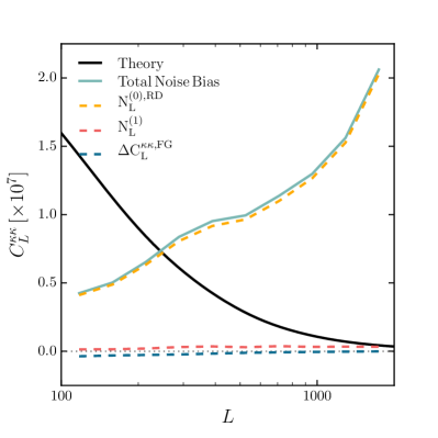
Figure 1.— Bias terms subtracted from the raw MV lensing spectrum: $N_{L}^{(0),\rm RD}$, $N_{L}^{(1)}$(converted to $C_{L}^{\kappa\kappa}$ units,  Eq. (12)), and foreground bias $\Delta C_{L}^{\kappa\kappa,{\rm FG}}$. The theoretical lensing convergence spectrum for the fiducial cosmology is shown in black. The disconnected term in the CMB 4-point function $N_{L}^{(0),\rm RD}$ is shown in dashed yellow (Eq. (8)). The spurious correlated power between the CMB and the lensing potential $N_{L}^{(1)}$ is shown in dashed pink (Eq. (9)). The sum of these two terms is labeled “Total Noise Bias” in the figure in solid green. The foreground bias from the tSZ trispectrum, CIB trispectrum, and the tSZ and CIB correlation with $\kappa$ is shown in dashed dark blue (Section 3.3). The total noise bias is also an estimate of the noise in the reconstructed $\phi$ map. Lensing modes with values of $L$ for which the total bias is less than the signal spectrum are measured at signal-to-noise greater than unity. For this measurement, that includes all modes with $L\lesssim$ 250, or angular scales of roughly a degree and larger.

We estimate the disconnected term using a realization-dependent method ($N_{L}^{(0),\rm RD}$, Namikawa et al. 2013). The standard $N_{L}^{(0)}$ is estimated by computing the lensing spectra with two input maps that form $\hat{\phi}$ from different simulation realizations. Since input maps from different realizations do not share the lensing potential, the resultant power in the lensing spectra comes from spurious correlations of the maps. With the realization-dependent method, we use a combination of simulation and data maps. Specifically, on top of the mix of simulation realizations, we also construct lensing potentials using data in one of the input maps. Accounting for all the different combinations, we have

$$N_{L}^{(0),\rm RD}=\\ \begin{aligned} \Big{\langle}&+C^{\hat{\phi}\hat{\phi}}_{L}[\bar{U}_{\rm d},\bar{V}_{\rm MC},\bar{X}_{\rm d},\bar{Y}_{\rm MC}]+C^{\hat{\phi}\hat{\phi}}_{L}[\bar{U}_{\rm MC},\bar{V}_{\rm d},\bar{X}_{\rm d},\bar{Y}_{\rm MC}]\\ &+C^{\hat{\phi}\hat{\phi}}_{L}[\bar{U}_{\rm d},\bar{V}_{\rm MC},\bar{X}_{\rm MC},\bar{Y}_{\rm d}]+C^{\hat{\phi}\hat{\phi}}_{L}[\bar{U}_{\rm MC},\bar{V}_{\rm d},\bar{X}_{\rm MC},\bar{Y}_{\rm d}]\\ &-C^{\hat{\phi}\hat{\phi}}_{L}[\bar{U}_{\rm MC},\bar{V}_{\rm MC^{\prime}},\bar{X}_{\rm MC},\bar{Y}_{\rm MC^{\prime}}]\\ &-C^{\hat{\phi}\hat{\phi}}_{L}[\bar{U}_{\rm MC},\bar{V}_{\rm MC^{\prime}},\bar{X}_{\rm MC^{\prime}},\bar{Y}_{\rm MC}]\Big{\rangle}_{\rm MC,MC^{\prime}}\,,\end{aligned}$$ (8)

where $C^{\hat{\phi}^{UV}\hat{\phi}^{XY}}_{L}$ is expressed as $C^{\hat{\phi}\hat{\phi}}_{L}[\bar{U},\bar{V},\bar{X},\bar{Y}]$ to more clearly indicate the sources of the input maps. Here $MC$ and $MC^{\prime}$ denote simulation skies from different realizations, and $d$ denotes the data map. The realization-dependent method produces a better estimate of the disconnected term because it reduces the bias from the mismatch between the fiducial cosmology used for generating the simulations and that in the data. In addition, this method reduces the covariance between the lensing potential bandpowers.

The second bias term $N_{L}^{(1)}$ comes from spurious correlations between the CMB and the lensing potential and is proportional to $C_{L}^{\phi\phi}$. We estimate it using pairs of simulated skies that have different realizations of unlensed CMB lensed with the same $\phi$:

$$N_{L}^{(1)}=\\ \begin{aligned} \Big{\langle}&+C^{\hat{\phi}\hat{\phi}}_{L}[\bar{U}_{\phi^{1},{\rm MC}},\bar{V}_{\phi^{1},{\rm MC^{\prime}}},\bar{X}_{\phi^{1},{\rm MC}},\bar{Y}_{\phi^{1},{\rm MC^{\prime}}}]\\ &+C^{\hat{\phi}\hat{\phi}}_{L}[\bar{U}_{\phi^{1},{\rm MC}},\bar{V}_{\phi^{1},{\rm MC^{\prime}}},\bar{X}_{\phi^{1},{\rm MC^{\prime}}},\bar{Y}_{\phi^{1},{\rm MC}}]\\ &-C^{\hat{\phi}\hat{\phi}}_{L}[\bar{U}_{\rm MC},\bar{V}_{\rm MC^{\prime}},\bar{X}_{\rm MC},\bar{Y}_{\rm MC^{\prime}}]\\ &-C^{\hat{\phi}\hat{\phi}}_{L}[\bar{U}_{\rm MC},\bar{V}_{\rm MC^{\prime}},\bar{X}_{\rm MC^{\prime}},\bar{Y}_{\rm MC}]\Big{\rangle}_{{\rm MC,MC^{\prime}}}\,,\end{aligned}$$ (9)

where the subscript $\phi^{1}$ denotes CMB maps lensed by the same $\phi$ realization.

We account for biases to the lensing spectrum due to foregrounds in the temperature map. As studied in van Engelen et al. (2014), both tSZ and CIB have a trispectrum, which leads to a response in the lensing power spectrum. This bias enters the lensing spectrum through the 4-point function of the temperature map, thus modifying the T spectrum and the MV spectrum. Additionally, since both tSZ and CIB trace the same large-scale structure as the lensing field, the non-Gaussianities of both fields can mimic lensing and couple through the $\phi$ estimator in a coherent way that correlates with $\phi$, forming a nonzero bispectrum of the matter density field (denoted by tSZ²-$\kappa$ and CIB²-$\kappa$). This effect biases the MV lensing spectrum and spectra from pairs of estimators of the form $\left<\phi^{TT}\phi^{UV}\right>$, where $UV\in[TT,TE,EE,EB,TB]$. The level of foreground bias is scale dependent. It is negative and close to flat at $\sim$2% for $L<1300$ for the total bias contributed from tSZ and CIB through their trispectra and correlations with $\phi$. As $L$ increases, the magnitude of this bias decreases and reaches a null at about $L$ of 2000. We subtract the relevant terms from the T and MV spectra by using the bias estimates from van Engelen et al. (2014). Specifically, we subtract the total foreground bias coming from the tSZ trispectra, CIB trispectra, tSZ²-$\kappa$, and CIB²-$\kappa$ from the T lensing spectrum. For the MV spectrum, we subtract the total foreground bias that enters through $\left<\phi^{TT}\phi^{TT}\right>$, and tSZ²-$\kappa$ and CIB²-$\kappa$ biases that enter through $\left<\phi^{TT}\phi^{UV}\right>$ with $UV\in[TE,EE,EB,TB]$. We compute the bias fraction by forming a weighted average of the foreground biases to $\left<\phi^{TT}\phi^{TT}\right>$ and $\left<\phi^{TT}\phi^{UV}\right>$. We use as weights the fractional contribution of the estimators to the MV estimator. The size of this bias in the MV spectrum is shown in Figure 1.

MC bias describes the difference between the recovered amplitude in simulations and the input spectrum. It is typically found to be small (e.g. Sherwin et al., 2017; Planck Collaboration et al., 2018b). In S15, we found that the mean MV amplitude $A_{\rm MV}$ from simulations was 3% below unity and treated this discrepancy as a source of systematic uncertainty. In this work, we find that the main source of our MC bias comes from the inclusion of the point source and cluster mask. When analyzing the set of simulations with the source mask removed (while keeping the boundary mask), we are able to recover $A_{\rm MV}=1$ to within 1 $\sigma$ of the standard error of 400 sky realizations ($0.058/\sqrt{400}=0.0029$) for the multipole range we report in this work. Furthermore, comparing the mean recovered spectrum of the MV, POL, and T estimators with and without the source mask applied to the input maps, we observe a relatively constant multiplicative offset in the range of $100<L\lesssim 800$. We therefore conclude that the main source of our MC bias is due to higher-order coupling generated from the presence of source masks in the map that is not accounted for by $f_{\rm mask}$. We construct a multiplicative correction for this MC bias $f_{\rm PS}$ as an inverse of the mean of the simulation lensing amplitudes $A_{\rm lens}$ estimated from $100<L<602$:

$$f^{XY,UV}_{\rm PS}={\langle A^{XY,UV}_{\rm lens}\rangle}^{-1}\,.$$ (10)

To check the stability of this estimate, we vary the maximum $L$ range used between $L$ of 446 and 813 and find the resultant simulation $A_{\rm lens}$ from all pairs of estimators to be consistent with unity to within 2 $\sigma$ of their standard errors. The correction from this step is about 5%. Specifically, $f_{\rm PS}$ for the MV, POL, and T are $f^{\rm MV}_{\rm PS}$ = 1.05, $f^{\rm POL}_{\rm PS}$ = 1.05, and $f^{\rm T}_{\rm PS}$ = 1.07. For $L<100$, the mean of the simulation spectra with the source mask removed is $5-10\%$ below the input spectrum. Therefore, this MC bias correction is not applicable for multipoles below 100, and we do not report results below $L$ of 100.

Figure 2.— Lensing $\kappa$ map reconstructed from the SPTpol 500 deg² field data, smoothed by a 1-degree FWHM Gaussian to highlight the signal-dominated modes. Top: The $\kappa$ map from the MV lensing estimator, which combines all temperature and polarization information. Bottom: $\kappa$ maps from the temperature estimator (T, left) and from combining the polarization estimators $EE$ and $EB$ (POL, right). At the angular scales shown, the POL estimator recovers the lensing potential with slightly higher S/N than the T estimator. Therefore, it has higher weight in the MV combination and traces the fluctuations of the MV $\kappa$ map with higher fidelity.

In constructing our simulations and applying the quadratic estimator to recover the lensing potential, we have assumed $\phi$ to be Gaussian. However, nonlinear structure growth and post-Born lensing would introduce non-Gaussianities to $\phi$ (Böhm et al., 2016; Pratten & Lewis, 2016). These non-Gaussianities produce the so-called $N_{L}^{(3/2)}$ bias, as studied in Böhm et al. (2016, 2018); Beck et al. (2018). For the $L$ range considered, the size of this bias is $\sim$0.5% for the temperature reconstruction and is negligible for the $EB$ reconstruction for input CMB maps similar in noise levels and multipole range to those in this work (Böhm et al., 2018; Beck et al., 2018). These are small compared with our other sources of uncertainties, and we neglect them in our results.

We report our results in binned bandpowers. First, we derive the per-bin amplitude as the ratio of the unbiased lensing spectrum to the input theory spectrum:

$$A_{b}^{UVXY}\equiv\frac{C^{\phi^{UV}\phi^{XY}}_{b}}{C^{\phi\phi,{\rm theory}}_{b}}\,,$$ (11)

with the subscript $b$ denoting a binned quantity; $C_{b}$ is a weighted average of the $C_{L}$ inputs for $L$ inside the boundaries of the bin, with the weights $w$ designed to maximize signal-to-noise: $w^{UV,XY}_{L}=C^{\phi\phi,{\rm theory}}_{L}/{\rm Var}(C^{\hat{\phi}^{UV}\hat{\phi}^{XY}}_{L})$. We obtain the variance from the corresponding set of simulation cross spectra.

We report the bandpowers in lensing convergence ($\kappa$) instead of the lensing potential $\phi$. The convergence field is $-1/2$ of the divergence of the deflection field, which is the gradient of the lensing potential $\phi$ (Lewis & Challinor, 2006):

$$\kappa=-\frac{1}{2}\nabla^{2}\phi\,.$$ (12)

In Fourier space, they are related by $\kappa_{L}=(L(L+1))\phi_{L}/2$. The reported bandpowers are derived as the product of the data amplitude $A_{b}$ and the input theory spectrum at bin center $L_{b}$,

$$\hat{C}^{\kappa\kappa}_{L_{b}}\equiv\frac{(L_{b}(L_{b}+1))^{2}}{4}A_{b}\,C^{\phi\phi,{\rm theory}}_{L_{b}}\,.$$ (13)

The overall lensing amplitude for each estimator is calculated identically as the per-bin amplitude in Eq. (11) using the whole reported $L$ range.

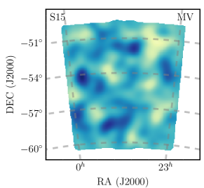
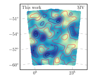
Figure 3.— Comparison with the S15 $\kappa$ map: Left: The $\kappa$ map reconstructed by S15 using the MV estimator with maps from SPTpol 100 deg² field observations (the sign is opposite from that shown in S15 because of a sign error in plotting in S15). Right: Cutout of the 100 deg² field from the MV $\kappa$ map in this analysis, overlaid with contours from the S15 MV $\kappa$ at $[-0.048,-0.032,-0.016,0,0.016,0.032,0.048]$. Both maps are smoothed by a 1-degree FWHM Gaussian. Data that enter the S15 reconstruction were taken before the 500 deg² survey, and thus are independent from the data used in this analysis. Since modes shown are measured to S/N greater than unity, the fluctuations of the two maps visually tracing each other serves as a consistency check.

Differences between the fiducial cosmology and the cosmology of the SPTpol patch would produce different measured lensing amplitudes. The cosmology dependence enters through the $N_{L}^{(1)}$ bias. In this work, since we choose a fiducial cosmology that is consistent with the data, we expect the difference in the $N_{L}^{(1)}$ bias to be small. To test this, we sample the lensing amplitude given the fiducial cosmology with and without corrections to $N_{L}^{(1)}$. We find the difference in the lensing amplitude for the MV estimator to be 0.007 (0.1 $\sigma$). We therefore neglect this correction in this work.

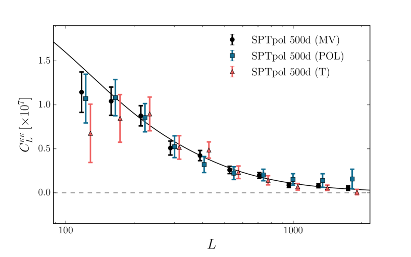
Figure 4.— Lensing convergence bandpowers estimated from SPTpol 500 deg² field data. We show bandpowers from the MV, POL, and T estimators. The POL and T bandpowers are shifted in $L$ for clarity. The T and POL bandpowers are consistent with each other given the errorbars of the bandpowers. The reconstruction noise of the POL estimator is lower than that of T for $L\lesssim 600$, and vice versa on smaller angular scales. This provides a sense of the angular scales at which each estimator gives better S/N. The black solid line shows the lensing convergence spectrum from the fiducial cosmology.

4. Results

In the following, we discuss our main results: the lensing convergence map, the lensing spectrum, and the lensing amplitude measurement. We compare our MV map to S15’s. We discuss the relative weights of the T and the POL results, compare the sizes of the systematic uncertainties to the statistical uncertainties, and put our measurement in the context of other lensing measurements.

In Figure 2, we show the MV, T, and POL lensing convergence. The maps are smoothed by a 1-degree FWHM Gaussian to highlight the higher signal-to-noise modes at the larger scales. At the angular scales shown, the POL reconstruction has higher signal-to-noise (lower $N_{L}^{(0)}$) than the T reconstruction. Therefore, while the T and the POL $\kappa$ map fluctuations both trace those in the MV map in broad strokes, we see that the POL modes trace the MV modes more faithfully. The lensing modes in the MV map are reconstructed with S/N better than unity for $L\lesssim 250$. It is the largest lensing map reconstructed with this S/N level from the CMB to date.

In Figure 3, we compare the MV $\kappa$ map from S15 and the one from this work over the same region of the sky. We observe that the two convergence maps show nearly identical degree-scale structure. The S15 data were taken before the SPTpol 500 deg² survey data (see Section 2.1), and thus constitute an independent dataset from that used in this work. In addition, because the two analyses have similar per-mode reconstruction noise, the visual agreement of the modes between the two is a useful consistency check.

Table 1MV lensing bandpowers

$[\,L_{\rm min}$	$L_{\rm max}\,]$	$L_{b}$	$10^{7}\hat{C}_{L_{b}}^{\kappa\kappa}$
$[\,100$	$133\,]$	$117$	$1.144\pm 0.230$
$[\,134$	$181\,]$	$158$	$1.041\pm 0.161$
$[\,182$	$244\,]$	$213$	$0.876\pm 0.115$
$[\,245$	$330\,]$	$288$	$0.509\pm 0.080$
$[\,331$	$446\,]$	$389$	$0.423\pm 0.058$
$[\,447$	$602\,]$	$525$	$0.260\pm 0.042$
$[\,603$	$813\,]$	$708$	$0.198\pm 0.032$
$[\,814$	$1097\,]$	$956$	$0.086\pm 0.025$
$[\,1098$	$1481\,]$	$1290$	$0.081\pm 0.023$
$[\,1482$	$1998\,]$	$1741$	$0.053\pm 0.025$

We present the lensing power spectrum measurement in logarithmically spaced bins in the range $100<L<2000$. We list the MV lensing bandpowers and their uncertainties in Table 1. The lower bound of the $L$ range is chosen by the region of validity of the MC bias correction. The upper bound is set by computing the uncertainties on the lensing amplitudes as we include higher multipoles and seeing no gain in signal-to-noise of the amplitude going beyond $L$ of 2000. In Figure 4, we show the bandpowers from the MV spectrum, the POL spectrum, and the T spectrum. We see that the error bars of the POL spectrum are smaller than those of the T spectrum at $L\lesssim 600$, and vice versa on smaller angular scales. This is consistent with the $N_{L}^{(0)}$ of the T reconstruction at small angular scales being lower than that of the POL reconstruction – the small angular scale modes are better reconstructed by the T estimator.

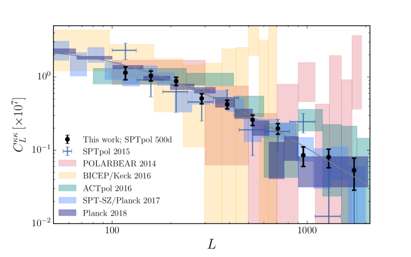
Figure 5.— Lensing power spectrum measurements from this work and S15 (MV) (Story et al., 2015), POLARBEAR (POL) (POLARBEAR Collaboration, 2014), BICEP2/Keck (POL) (Keck Array et al., 2016), ACTPol (MV) (Sherwin et al., 2017), SPT-SZ + Planck (T) (Omori et al., 2017), and Planck (MV) (Planck Collaboration et al., 2018b). The gray solid line is the lensing spectrum from the best-fit $\Lambda$CDM model to the Planck plikHM_TT_lowTEB_lensing dataset. This work contains data from $\sim$5 times more area than S15 and the sizes of the errorbars of the signal-dominated multipoles reflect the decrease in sample variance. In addition, it is the tightest lensing amplitude measurement of all the lensing measurements made using only ground-based telescope data to date.

We measure the overall lensing amplitude for each estimator and find

$$\begin{aligned} A_{\rm MV}&=0.944\pm 0.058{\rm\,(Stat.)}\pm 0.025{\rm\,(Sys.)}\,,\\ A_{\rm POL}&=0.906\pm 0.090{\rm\,(Stat.)}\pm 0.040{\rm\,(Sys.)}\,,\\ A_{\rm T}&=0.835\pm 0.103{\rm\,(Stat.)}\pm 0.012{\rm\,(Sys.)}\,.\end{aligned}$$

We derive the statistical uncertainties from the standard deviations of the lensing amplitudes from simulations. We detail the sources of systematic uncertainties in Section 5.2 and break them down in Table 3. Considering statistical uncertainties alone, we measure the lensing amplitude with $6\%$ uncertainty using the MV estimator and with $10\%$ uncertainty with the POL estimator. For the T estimator, we measure the lensing amplitude with $12\%$ uncertainty. Having chosen the same cuts in multipole space for both the input temperature and polarization maps, this shows that the signal-to-noise per mode in the input polarization maps are now high enough that the POL estimators give more stringent measurements of the lensing amplitude than the T estimator. In future analyses, the T lensing spectrum is sample-variance limited and cannot be improved by lowering the temperature map noise levels. Instead, it can be improved by including information from higher multipoles and/or more sky area. However, lowering the noise levels of the polarization maps can still improve the lensing measurement from polarization estimators. Specifically, unlike the temperature estimator, the $N_{L}^{(0)}$ of the $EB$ estimator is not limited by unlensed power in the map, because there is little unlensed $B$ mode power to contribute to $N_{L}^{(0)}$ in the multipole range important for lensing reconstruction. In addition to surpassing the measurement uncertainty of the T lensing amplitude, considering statistical uncertainties alone, our POL lensing amplitude is the most precise amplitude measurement ($10.1\,\sigma$) using polarization data alone to date.

The systematic uncertainties for the MV and the POL estimators are $\sim$40% of their respective statistical uncertainties, whereas the systematic uncertainty is subdominant for the T estimator compared with its statistical uncertainty. For both the MV and the POL estimators, the systematic uncertainty budget is dominated by the $P_{\rm cal}$ uncertainty (Section 5.2). Including the systematic uncertainties in the MV amplitude measurement, we measure $A_{\rm MV}$ with $7\%$ uncertainty.

We detect lensing at very high significance. From reconstructing $\phi$ using 400 unlensed simulations, the standard deviation of $A^{\rm unl}_{\rm MV}$ is 0.024. The observed amplitude of $A_{\rm MV}=0.944$ would thus correspond to a $39\,\sigma$ fluctuation.

Compared with other ground-based measurements, our result has the tightest constraint on the lensing amplitude. In Figure 5, we show our lensing power spectrum measurement against previous measurements. Our measurement is consistent with the measurement by Omori et al. (2017). In that work, they reconstruct lensing using a combined temperature map from SPT-SZ and Planck over the common 2500 deg² of sky. They measure the lensing amplitude to be $0.95\pm 0.06$ relative to the best-fit $\Lambda$CDM model to the Planck 2015 plikHM_TT_lowTEB_lensing dataset (same as the fiducial cosmology used in this work). The most recent lensing analysis of all-sky Planck data found the best-fit lensing amplitude to be $1.011\pm 0.028$ against the Planck 2018 TTTEEE_lowE_lensing cosmology (Planck Collaboration et al., 2018b). To compare our measurement with this model, we refit our minimum-variance bandpowers and get $A_{\rm MV}=0.946\pm 0.058{\rm\,(Stat.)}\pm 0.025{\rm\,(Sys.)}$, consistent with Planck’s lensing measurement.

5. Null Tests, Consistency Checks, and Systematic Uncertainties

In this section, we summarize the null and consistency tests we have performed on the data and account for the systematic uncertainties in our lensing amplitude measurements. We report test results from the MV, POL, and T estimators.

5.1. Null Tests and Consistency Checks

We quantify the results of our tests using summary statistics comparing data bandpower differences with simulation bandpower-difference distributions, where the differences are taken between bandpowers obtained from the baseline analysis pipeline and from a pipeline with one analysis change. We plot these bandpowers in Figure 6 to provide an absolute sense of how much the bandpowers and their error bars change given the various analysis variations.

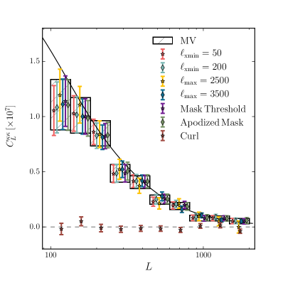
Figure 6.— Results of the power spectrum consistency tests and curl null test. The figure shows $C_{L}^{\kappa\kappa}$ bandpowers from different analysis choices and the curl test bandpowers. The MV bandpowers and errorbars from the baseline analysis are plotted as boxes. The bandpowers calculated with different analysis choices are consistent with the baseline MV bandpowers. The bandpowers from the curl null test are consistent with zero.

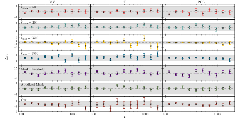
Figure 7.— The difference bandpowers ($\Delta C_{L}^{\kappa\kappa}$) and their uncertainties between the baseline analysis and analyses with one change as indicated in the labels, scaled by the uncertainties of the respective MV, T, POL bandpowers. The 1 $\sigma$ bands of the MV, T, and POL estimators are shaded in gray. This is a visual summary of the $\chi^{2}$ values listed in Table 2. We find the analysis-variation bandpowers and best-fit lensing amplitudes to be consistent with the baseline setup for all three estimators.

Quantitatively, we calculate the $\chi^{2}$ of the data-difference spectrum $(\Delta C^{\phi\phi}_{b,\,{\rm data}})$ against the mean of the simulation-difference spectrum $(\langle\Delta C^{\phi\phi}_{b,\,{\rm sim}}\rangle)$ using the variance of the simulation-difference spectra ($\sigma_{b,\,{\rm sys}}^{2}$), as the difference bandpowers are largely uncorrelated:

$$\chi^{2}_{\rm sys}=\sum_{b}{\frac{(\Delta C^{\phi\phi}_{b,\,{\rm data}}-\langle\Delta C^{\phi\phi}_{b,\,{\rm sim}}\rangle)^{2}}{\sigma_{b,\,{\rm sys}}^{2}}}\,.$$ (14)

The probability-to-exceed (PTE) is calculated from a $\chi^{2}$ distribution with 10 degrees of freedom, as we have 10 bandpowers. For the curl test, $\sigma_{b,\,{\rm sys}}$ comes from the distribution of the simulation curl spectra. Figure 7 provides a visual summary of these tests. It shows the data-difference bandpowers for each test for the three estimators. The error bars are generated from the distributions of simulation-difference bandpowers. The data points and the error bars from each estimator in each $L$ bin are scaled by the 1 $\sigma$ lensing spectrum uncertainties from that estimator in that bin. We list the $\chi^{2}$ and PTE values for each test and each estimator in Table 2.

We compare the differences in overall lensing amplitude similarly. We calculate the difference in the lensing amplitudes between the baseline and the alternate analysis choice setup: $\Delta A_{\rm data}$. We form the $\chi^{2}$ by comparing the data-difference amplitude against the distribution of the difference amplitudes in simulations.

Table 2Consistency and Null tests $\chi^{2}$ and PTE

Test Name $\chi^{2}_{\rm MV}$ (PTE) $\Delta$ $A_{\rm MV}$ (PTE) $\chi^{2}_{\rm T}$ (PTE) $\Delta$ $A_{\rm T}$ (PTE) $\chi^{2}_{\rm POL}$ (PTE) $\Delta$ $A_{\rm POL}$ (PTE) $\pm{\rm var}(\Delta A_{\rm MV})$ $\pm{\rm var}(\Delta A_{\rm T})$ $\pm{\rm var}(\Delta A_{\rm POL})$ $\ell_{\rm xmin}$=50 7.2 (0.71) -0.002 $\pm$ 0.013 (0.76) 5.8 (0.83) 0.005 $\pm$ 0.019 (0.86) 9.7 (0.47) -0.015 $\pm$ 0.025 (0.55) $\ell_{\rm xmin}$=200 4.3 (0.93) 0.017 $\pm$ 0.021 (0.44) 10.4 (0.40) 0.035 $\pm$ 0.026 (0.17) 3.3 (0.97) -0.005 $\pm$ 0.037 (0.90) $\ell_{\rm max}$=2500 14.2 (0.17) -0.000 $\pm$ 0.035 (0.98) 12.0 (0.28) 0.040 $\pm$ 0.093 (0.65) 5.9 (0.83) -0.021 $\pm$ 0.018 (0.25) $\ell_{\rm max}$=3500 17.2 (0.07) 0.014 $\pm$ 0.023 (0.66) 8.2 (0.61) 0.085 $\pm$ 0.055 (0.17) 11.0 (0.36) -0.006 $\pm$ 0.008 (0.48) Mask thres. 13.2 (0.21) 0.006 $\pm$ 0.008 (0.43) 15.6 (0.11) 0.021 $\pm$ 0.014 (0.10) 14.6 (0.15) -0.002 $\pm$ 0.013 (0.88) Apod. mask 4.8 (0.91) 0.004 $\pm$ 0.012 (0.90) 13.3 (0.20) 0.035 $\pm$ 0.022 (0.13) 3.7 (0.96) -0.002 $\pm$ 0.022 (0.85) Curl 9.3 (0.50) -0.007 $\pm$ 0.005 (0.20) 7.5 (0.67) -0.013 $\pm$ 0.013 (0.29) 9.4 (0.49) -0.010 $\pm$ 0.009 (0.28)

Varying $\ell_{\rm xmin}$ and $\ell_{\rm max}$: We vary the multipole range of the input CMB maps used for lensing reconstruction to check the following: (1) consistency of bandpowers as we include more or fewer CMB modes and (2) impact of foregrounds as we increase the maximum multipole. As we increase the maximum multipole used in the input temperature map, the contamination of the CMB by foregrounds like tSZ and CIB increases. As discussed in Section 3.3, both of these inputs can bias the lensing spectrum. On the low $\ell$ side, we remove $|\boldsymbol{\ell}_{x}|<\ell_{\rm xmin}$ modes because the combination of our observing strategy and time stream filtering removes modes approximately along the $\ell_{x}=0$ axis. We run two cases for the $\ell_{\rm xmin}$ cut: $\ell_{\rm xmin}=50$ and $\ell_{\rm xmin}=200$. From  Table 2, we see that the differences of the $\ell_{\rm xmin}$ cases are consistent with the expected simulation distribution. We can in principle set the $\ell_{\rm xmin}$ in the baseline analysis to be 50. However, since the applied time stream filtering removes $\ell\lesssim 100$ modes, and the number of modes available between $\ell_{\rm xmin}$ of 50 and 100 is small compared with the number of modes at the high-$\ell$ end, we do not expect there to be significant improvement in signal-to-noise and therefore choose to set $\ell_{\rm xmin}=100$ for the baseline analysis. For the $\ell_{\rm max}$ tests, we vary the $\ell_{\rm max}$ cut between $\boldsymbol{\ell}=2500$ and $\boldsymbol{\ell}=3500$ in steps of 500. We observe from Table 2 that moving between $\ell_{\rm max}$ of 3000 and 2500 and between $\ell_{\rm max}$ of 3000 and 3500, the data bandpower differences are consistent with bandpower differences from simulations for all three sets of estimators. We set the baseline $\ell_{\rm max}$ to be 3000 to keep the systematic uncertainty due to the subtraction of foreground biases subdominant to the statistical uncertainty of the measurements. For future analyses, estimators designed to reduce foreground biases (Osborne et al., 2014; Schaan & Ferraro, 2019; Madhavacheril & Hill, 2018) can be employed, potentially sacrificing some statistical power for reduced systematic uncertainty.

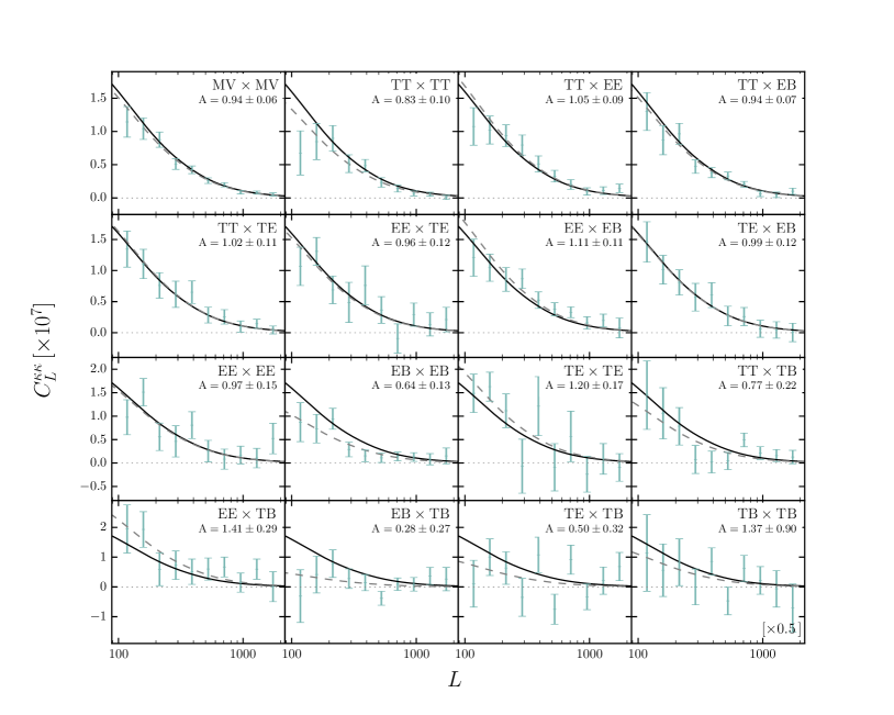
Figure 8.— Comparison of cross-spectra of individual estimators and the minimum variance combination MV$\times$MV. The lensing spectrum from the fiducial cosmology, the Planck plikHM_TT_lowTEB_lensing $\Lambda$CDM best fit, is plotted in solid black. The best fit from each estimator is plotted in dashed gray. The amplitudes are computed relative to the fiducial lensing spectrum. The data points and errorbars are scaled by 0.5 for the TB$\times$TB spectrum to allow all the points to be shown. We find a ${\rm PTE}=0.44$ when comparing the 150 bandpowers against the best fit of the MV spectrum using a covariance matrix constructed from simulations.

Source masking threshold: We check the impact of extragalactic foregrounds on the lensing measurements by varying the masking thresholds of point sources and galaxy clusters. We raise the thresholds of the point source and the cluster masks so that about 20% more sources are kept in the input maps. The modified cuts correspond to a flux threshold of 7.5 mJy and a cluster detection significance threshold of 4.7, whereas the baseline thresholds (see Section 2.2) are 6 mJy and 4.5 (i.e., the threshold for inclusion in the Bleem et al. 2015 catalog). From the bandpower PTEs and amplitude PTEs listed in Table 2, we see that the differences in bandpowers and amplitudes are consistent with expected variations from simulations. Therefore, we conclude that the masking thresholds we apply in the baseline analysis reduce foreground biases to the lensing spectrum sufficiently.

Apodization: We test for the effects of using a top hat function for the boundary and source mask by redoing the entire analysis using a cosine taper instead. The radius of the cosine taper is 10^′ for the boundary mask and 5^′ for the sources. The data difference is typical given the simulation-difference distribution for all three estimators.

Curl test: The deflection field $\mathbb{d}(\hat{\mathbb{n}})$ that remaps the primordial CMB anisotropies can be generically decomposed into a gradient and a curl component:

$$\mathbb{d}(\hat{\mathbb{n}})=\nabla\phi(\hat{\mathbb{n}})+\star\nabla\Omega(\hat{\mathbb{n}})\,,$$ (15)

where $\star$ is a 90^∘ rotation operator and $\Omega(\hat{n})$ is a psuedo-scalar field that sources the curl component (see e.g. Hirata & Seljak, 2003; Namikawa et al., 2012). In the Born approximation, the lensing potential only sources the gradient component of the deflection field. At current noise levels and barring unknown physics, the curl component is expected to be consistent with zero. Therefore, estimating the curl of the deflection field serves as a test of the existence of any components in the data generated from non-Gaussian secondary effects or foregrounds (Cooray et al., 2005). Analogous to estimating the lensing $\phi$ field, for the curl component, we estimate the psuedo-scalar field $\Omega$. The curl estimator is orthogonal to the lensing (gradient) estimator and has the same form as the lensing estimator Eq. (1). The weights of the curl estimator are designed to have response to the curl instead of the gradient. We implement the weights as presented in Namikawa et al. (2012). The curl spectrum is derived analogous to the lensing spectrum with two differences: (1) the theory input is set to a flat spectrum $C_{L}^{\Omega\Omega}=10^{-7}$, where it is used for uniformly weighting the modes when binning and as a reference spectrum for the amplitude calculation; (2) no response correction from simulations is applied to the psuedo-scalar field as the expected signal is zero. The bottom panel of Figure 7 shows the power spectra for the MV, POL, and T curl estimators and their uncertainties scaled by the respective uncertainties of their lensing spectra. The bandpower PTEs and the amplitude PTEs for the three estimators are listed in Table 2. They are all consistent with zero. The bandpower PTE and the amplitude PTE are 0.50 and 0.20 for the MV curl estimator. We thus see no evidence of contamination to our lensing estimate from non-Gaussian secondaries.

Consistency across estimators: In Figure 8, we show the reconstructed lensing spectrum from all 15 pairs of the 5 estimators $TT,TE,EE,EB,TB$, and the MV spectrum. We test for consistency of the lensing spectra from the 15 pairs of estimators with the best fit from the MV estimator by calculating $\chi^{2}$ and PTE. We calculate the $\chi^{2}$ of the 150 bandpowers against the binned theory spectrum scaled by the best-fit MV amplitude:

$$\chi^{2}=(d-m)\,{\rm Cov}^{-1}(d-m)^{\dagger}\,,$$ (16)

where $d$ is the 150 data bandpowers, $m$ is 15 copies of the scaled binned theory spectrum, and ${\rm Cov}$ denotes the covariance matrix. We construct the covariance matrix of the 150 bandpowers of 15 estimators from 400 simulations. We set the off-diagonal terms of each subblock off the main diagonal to zero as we expect there to be and have verified that there is little to no correlation across different $L$ bins between estimators. For the main diagonal, the first and second bins are correlated at the $\sim$10% level for 12 of the estimators, and we keep them while setting the rest of the covariance elements to zero. The PTE compared to the set of 400 sets of simulated bandpowers is 0.44. Comparing instead the best-fit amplitudes of the 15 pairs of estimators with the MV best-fit amplitude, we note that the EB$\times$TB and EB$\times$EB pairs are low by 2.4 $\sigma$ and 2.1 $\sigma$ respectively, while the rest of the pairs are within 2 $\sigma$ of the MV’s amplitude. With the number of tests we have performed, it is not unusual to see 2 $\sigma$ outliers.

5.2. Systematic Uncertainty

In this section, we summarize the sources of systematic uncertainty and our accounting of them in the lensing amplitude measurement. We quantify the uncertainties in the lensing amplitude measurement due to uncertainties in the beam measurement, temperature and polarization calibrations, T$\rightarrow$P leakage correction, global polarization angle rotation, and the applied foreground template. We address the potential impact of non-Gaussian polarized foregrounds. The sources of systematic uncertainty and their respective impact on the lensing amplitude measurements are listed in Table 3.

Beam uncertainty: We take the beam measurement uncertainty $\Delta B_{\ell}$ derived from the beam covariance matrix in H18 and convolve (1+ $\Delta B_{\ell}$) with the input $\bar{X}$ maps while keeping all the simulation maps the same. We analyze the data maps as if their beam were the mean measured beam $B_{\ell}$ as opposed to the modified $B_{\ell}(1+\Delta B_{\ell})$. The difference in the lensing amplitude between this analysis and the baseline analysis quantifies the effect of an underestimation of the beam profile by 1 $\sigma$ of the beam measurement uncertainty across the entire angular multipole range. We find $\Delta A_{\rm MV}=0.008$, $\Delta A_{\rm POL}=0.010$, and $\Delta A_{\rm T}=0.005$. The systematic uncertainties induced by the beam uncertainty are small ($\sim$0.1 $\sigma$) compared with the respective statistical uncertainties of the measured lensing amplitudes in T, POL, and MV.

Temperature and polarization calibrations: We apply the temperature and polarization calibration factors derived in H18 to our data $T/Q/U$ maps as described in Section 2.2. From the posterior distributions of H18, we obtain the uncertainties of the $T_{\rm cal}$ factor $\delta$$T_{\rm cal}$ and the $P_{\rm cal}$ factor $\delta$$P_{\rm cal}$  which are 0.3% and 0.6% respectively. The $T_{\rm cal}$ and $P_{\rm cal}$ are applied to the raw temperature and polarization maps through $T=T^{\rm raw}\times$ $T_{\rm cal}$ and $(Q/U)=(Q/U)^{\rm raw}\times$ $T_{\rm cal}$$\times$ $P_{\rm cal}$. Keeping the simulated maps fixed to the baseline analysis, we scale the data maps by $(1+\delta$$T_{\rm cal}$) for the temperature map and (1+$\delta$$T_{\rm cal}$)(1+$\delta$$P_{\rm cal}$) for the polarization maps and we recalculate the data lensing amplitudes. The two pieces in the amplitude calculation that change because of the modified data maps are $C^{\hat{\phi}\hat{\phi}}_{L}$ and $N_{L}^{(0),\rm RD}$. To illustrate how they contribute to the overall change in the lensing amplitude, we consider here the temperature-only estimator. $C^{\hat{\phi}\hat{\phi},T}_{L}$, which contains four copies of the data map, would shift by $(1+\delta T_{\rm cal})^{4}$. For $N_{L}^{(0),\rm RD}$, the four terms where two of the four input maps are replaced by data maps get a multiplicative correction of $(1+\delta T_{\rm cal})^{2}$. The overall shift in $\hat{C}^{\phi\phi,T}_{L}$ is therefore

$$\Delta\hat{C}^{\phi\phi}_{L}=\Delta C^{\hat{\phi}\hat{\phi}}_{L}-\Delta N_{L}^{(0),\rm RD}\,,$$ (17)

where

$$\Delta C^{\hat{\phi}\hat{\phi}}_{L}=[(1+\delta T_{\rm cal})^{4}-1]C^{\hat{\phi}\hat{\phi}}_{L}\simeq 4\delta T_{\rm cal}\,C^{\hat{\phi}\hat{\phi}}_{L}$$ (18)

and

$$\begin{aligned} \Delta N_{L}^{(0),\rm RD}\simeq 2\delta&{\rm T_{cal}}\,\big{\langle}\,C^{\hat{\phi}\hat{\phi}}_{L}[\bar{T}_{\rm d},\bar{T}_{\rm MC},\bar{T}_{\rm d},\bar{T}_{\rm MC}]\\ &\quad+C^{\hat{\phi}\hat{\phi}}_{L}[\bar{T}_{\rm MC},\bar{T}_{\rm d},\bar{T}_{\rm d},\bar{T}_{\rm MC}]\\ &\quad+C^{\hat{\phi}\hat{\phi}}_{L}[\bar{T}_{\rm d},\bar{T}_{\rm MC},\bar{T}_{\rm MC},\bar{T}_{\rm d}]\\ &\quad+C^{\hat{\phi}\hat{\phi}}_{L}[\bar{T}_{\rm MC},\bar{T}_{\rm d},\bar{T}_{\rm MC},\bar{T}_{\rm d}]\,\big{\rangle}_{\rm MC}\,,\\ \end{aligned}$$ (19)

with ${\rm MC}$ denoting simulation realizations and $d$ denoting data. The polarization-only case has a similar form as the temperature-only case with $(1+\delta T_{\rm cal})\rightarrow(1+\delta T_{\rm cal})(1+\delta P_{\rm cal})$. The difference in the resultant measured amplitudes due to an offset in the calibration factors depends on the relative amplitudes of $C^{\hat{\phi}\hat{\phi}}_{L}$ and $N_{L}^{(0),\rm RD}$ at each multipole $L$. Therefore, we quantify the difference by running the baseline analysis with the temperature and polarization calibration of the data maps shifted by 1 $\sigma$. We find that $\Delta A_{\rm MV}=0.023$, $\Delta A_{\rm POL}=0.039$, and $\Delta A_{\rm T}=0.008$. The shifts in the lensing amplitudes are dominated by the polarization calibration uncertainty. Furthermore, the calibration systematic uncertainty is almost half of the statistical uncertainty of the polarization-only amplitude. Since the signal-to-noise of future lensing measurements will be driven by the polarization estimators, we will need more precise polarization calibration in order for the measurements to remain dominated by statistical uncertainties. This can be achieved by cross-calibrating with deeper CMB maps or over larger areas of sky, assuming an external CMB map exists with more accurate polarization calibration than Planck. Relatedly, lensing measures mode coupling which in principle can be extracted irrespective of the input maps calibration. An example of circumventing the systematic uncertainty contribution caused by calibration uncertainties in the input maps is to use the measured power spectra in one of the weight functions in the analytic response in Eq. (2). In this approach, the response moves together with the calibration of the input maps and therefore eliminates this systematic uncertainty.

Temperature-to-polarization leakage: We estimate the bias to the lensing amplitude measurement caused by misestimating the T$\rightarrow$P leakage factors. Similar to quantifying the systematic offsets by the beam uncertainty and the $T_{\rm cal}$/$P_{\rm cal}$ uncertainties, here we modify the data polarization maps by over-subtracting a $\epsilon^{(Q/U)}$-scaled copy of the temperature map by 1 $\sigma$ in $\epsilon^{Q}$ and $\epsilon^{U}$, while keeping the rest of the analysis the same. We find the change in $A_{\rm MV}$ and $A_{\rm POL}$ to be negligible, at 0.001 $\sigma$ and 0.002 $\sigma$ respectively.

Global polarization angle rotation: There is a 6% uncertainty in the global rotation angle measured through the minimization of the $TB$ and $EB$ spectra discussed in Section 2.2. How much would an offset in the polarization angle rotation bias the lensing amplitude measurement? We run the baseline analysis with the data polarization maps rotated an extra 6% on top of the measured angle from the minimization procedure. We find that $A_{\rm MV}$ and $A_{\rm POL}$ change by less than 0.01 $\sigma$ of their respective statistical uncertainties.

Extragalactic foregrounds: As discussed in Section 3.3, we subtract templates of expected foreground biases from the T and MV lensing power spectra $\hat{C}^{\phi\phi}_{L}$ given models of CIB and tSZ from van Engelen et al. (2014). The templates are taken from the mean of the range of models. We estimate the systematic uncertainty from the template subtraction step by measuring the lensing amplitude difference using the maximum and minimum of template values allowed by the model space. We find the lensing amplitudes $A_{\rm MV}$ to shift by $\pm 0.004$ and $A_{\rm T}$ to shift by $\pm 0.008$, both less than 0.1 $\sigma$ of their statistical uncertainties. For the temperature estimator, this source of bias is $\sim$1% of the lensing amplitude and is of the same magnitude as the bias from the temperature calibration. For polarization, we expect the only significant source of extragalactic foregrounds to come from the unclustered point-source component, because SZ and the clustered CIB are negligibly polarized. The SZ effects are expected to be polarized at the less than 1% level for the cluster masking threshold of this work (Birkinshaw, 1999; Carlstrom et al., 2002). The clustered CIB component is a modulation of the mean power from all sources (Scott & White, 1999) and is thus effectively unpolarized. For the unclustered point sources, we measure the mean squared polarization fraction to be $\langle p^{2}\rangle=(\,0.95\pm 0.11\,)\times 10^{-3}$ ($\sim$3% polarized) at 150 GHz for sources above 6 mJy in the SPTpol field (Gupta et al., 2019). Assuming the polarization fraction is constant with flux density, the extragalactic foregrounds are thus on average significantly less polarized than the CMB. Since the level of bias introduced from temperature foregrounds is at the percent level, we conclude that the bias from polarized sources is negligible for this work.

Table 3Systematic Uncertainties

Type	$\Delta A_{\rm MV}$	$\Delta A_{\rm POL}$	$\Delta A_{\rm T}$
$\Delta A_{\rm beam}$	$0.008$	$0.010$	$0.005$
$\Delta A_{\rm cal}$	$0.023$	$0.039$	$0.008$
$\Delta A_{\rm T\rightarrow P}$	$\ll 0.001$	$\ll 0.001$	N/A
$\Delta A_{\rm pol.rot.}$	$<0.001$	$<0.001$	N/A
$\Delta A_{\rm fg}$	$0.004$	N/A	$0.008$
$\Delta A_{\rm tot}$	$0.025$	$0.040$	$0.012$

Galactic foregrounds: Galactic foregrounds are non-Gaussian and can contribute to both the lensing estimator, imparting a bias to the lensing spectrum measurement, and the curl estimator, causing the curl null test to fail. We mitigate these potential effects by (1) observing a low-foreground patch, (2) suppressing power from angular scales that are foreground dominated. We use the curl null test to check for potential contamination from galactic foregrounds. The SPTpol 500 deg² field is one of the lowest galactic foreground regions (e.g. Planck Collaboration et al., 2018d). Galactic foreground power is fainter than the CMB in both temperature and in $E$-mode polarization for the angular scales considered. However, polarized thermal dust dominates the $B$-mode power on angular scales below multipole $\ell$ of 200 (BICEP2 Collaboration et al., 2018). Challinor et al. (2018) showed that by including the foreground power spectrum as a noise term in the C^-1 filter of the input CMB fields, the polarization estimator can recover unbiased lensing amplitude to sub-percent accuracy. In this work, Galactic dust power in $EE$ and $BB$ at the same level as the simulation inputs are included as noise terms in the map filters. Finally, if Galactic foregrounds had been a significant source of bias, we would fail the curl null tests. The data pass the curl null test for the T, POL  and MV estimators, suggesting that biases from Galactic foregrounds are subdominant at present.

We summarize the systematic uncertainties contributed from each source addressed in this section in Table 3. We add the differences in lensing amplitude from each source in quadrature and include the result as a systematic uncertainty in our lensing amplitude measurements. The total systematic uncertainties are $A_{MV}^{\rm sys}=0.025$, $A_{\rm POL}^{\rm sys}=0.040$, and $A_{\rm T}^{\rm sys}=0.012$ respectively. The T systematic uncertainty is subdominant given the statistical uncertainties of the T lensing amplitude, while those for the MV and POL reach $\sim$0.4 $\sigma$ of their respective statistical uncertainties.

6. Conclusions

In this work, we present a new measurement of the CMB lensing potential from the 500 deg² SPTpol survey. We use a quadratic estimator to extract the lensing potential $\phi$ from combinations of temperature and polarization maps. Our per-mode measurement has signal-to-noise similar to that in S15 because the noise levels of the input maps are similar – we measure $\phi$ with signal-to-noise better than unity in the multipole range $100<L\lesssim 250$.

We measure the lensing amplitude with our minimum-variance combination of estimators to be $A_{\rm MV}=0.944\pm 0.058{\rm\,(Stat.)}\pm 0.025{\rm\,(Sys.)}$. Of the published lensing measurements using data only from ground-based telescopes, this is the tightest measurement of the lensing amplitude to date. Using unlensed simulations to estimate the probability of the measurement, we find that in the absence of true CMB lensing our measurement would be a $39\,\sigma$ outlier – i.e., we detect lensing at very high significance. We make individual combinations of temperature and polarization estimators. Considering statistical uncertainties alone, our polarization-only lensing constraint is the most precise amongst measurements of its kind to date. We perform null tests and consistency checks on our results and find no evidence for significant contamination. We estimate the size of the systematic uncertainty in our lensing measurement from uncertainties in calibration, beam measurement, T$\rightarrow$P leakage correction, global polarization rotation, and subtraction of extragalactic foreground bias. We find that our systematic uncertainty is nearly half as large as our statistical uncertainty and dominated by the uncertainty in the polarization calibration. Looking forward, we will have to either improve the precision of the polarization calibration or find solutions to self-calibrate the lensing estimator in order to reduce this systematic uncertainty.

The lensing spectrum measurement in this work is at sufficiently high precision to provide relevant independent constraints on cosmological parameters like $\Omega_{M}$, $\sigma_{8}$, and the sum of neutrino masses. We will report cosmological parameter constraints in a future paper. While this work represents the first analysis in which the lensing amplitude is better constrained by polarization, rather than temperature data, this will become typical for future experiments as map noise levels continue to decrease. The $EB$ estimator will eventually become the most constraining CMB lensing estimator, at least for lensing multipoles below several hundred. For the expected survey map depths of the currently operating SPT-3G experiment (3.0, 2.2, and 8.8 $\mu$K-arcmin at 95, 150, and 220 GHz respectively,  Bender et al. 2018), the $EB$ estimator is projected to provide the highest signal-to-noise lensing amplitude measurement of all pairs of input CMB maps.

The advantages of using polarization maps for CMB lensing measurements are as follows. First, foregrounds in CMB temperature maps, e.g. tSZ, are the main sources of bias in cross correlations with other dark matter tracers (Abbott et al., 2018b; Namikawa et al., 2019). Polarization maps are less contaminated by extragalactic foregrounds, and thus more modes on small angular scales (high $\ell$) can be used for lensing reconstruction and for cross correlation, improving the S/N of the measurement in addition to reducing foreground biases. Second, lensing estimators are typically limited by the $N_{L}^{(0)}$ noise contributed by the unlensed power in the input maps. The $EB$ estimator, however, is not as limited because unlensed $B$ power is subdominant to lensing $B$ power on subdegree scales. Furthermore, to first order in $\phi$, lensing $B$ modes are sourced completely by $E$ modes. These factors make methods beyond the quadratic estimator that approach the optimal solution (Millea et al., 2017) particularly efficient in improving the S/N of the $EB$ estimator.

High-S/N lensing measurements are essential for constraining the sum of neutrino masses and the amplitude of primordial gravitational waves, parameterized by the tensor-to-scalar ratio $r$. In the coming few years, the uncertainty on $r$ from upcoming CMB experiments will be limited by the variance of the lensing $B$ modes. To make progress in constraining $r$, we need lensing measurements with high S/N per mode for delensing (Manzotti et al., 2017). For example, delensing with the lensing map from SPT-3G will be crucial for the BICEP Array experiment (Hui et al., 2018) to reach its projected uncertainty on $r$ of $\sigma(r)\sim 0.003$, in which delensing improves $\sigma(r)$ by a factor of about 2.5. For the next-generation ground-based CMB experiment CMB-S4, delensing is even more crucial for achieving the projected $r$ constraint of $\sigma(r)=5\times 10^{-4}$ (CMB-S4 Collaboration et al., 2016).

References

- Abbott et al. (2018a) Abbott, T. M. C., Abdalla, F. B., Alarcon, A., et al. 2018a, Phys. Rev. D, 98, 043526, doi: 10.1103/PhysRevD.98.043526
- Abbott et al. (2018b) —. 2018b, arXiv e-prints, arXiv:1810.02322. https://arxiv.org/abs/1810.02322
- Beck et al. (2018) Beck, D., Fabbian, G., & Errard, J. 2018, Phys. Rev. D, 98, 043512, doi: 10.1103/PhysRevD.98.043512
- Bender et al. (2018) Bender, A. N., Ade, P. A. R., Ahmed, Z., et al. 2018, in Society of Photo-Optical Instrumentation Engineers (SPIE) Conference Series, Vol. 10708, Millimeter, Submillimeter, and Far-Infrared Detectors and Instrumentation for Astronomy IX, 1070803
- BICEP2 Collaboration et al. (2018) BICEP2 Collaboration, Keck Array Collaboration, Ade, P. A. R., et al. 2018, Physical Review Letters, 121, 221301, doi: 10.1103/PhysRevLett.121.221301
- Birkinshaw (1999) Birkinshaw, M. 1999, Physics Reports, 310, 97
- Blanchard & Schneider (1987) Blanchard, A., & Schneider, J. 1987, A&A, 184, 1
- Bleem et al. (2015) Bleem, L. E., Stalder, B., de Haan, T., et al. 2015, ApJS, 216, 27, doi: 10.1088/0067-0049/216/2/27
- Böhm et al. (2016) Böhm, V., Schmittfull, M., & Sherwin, B. D. 2016, Phys. Rev. D, 94, 043519, doi: 10.1103/PhysRevD.94.043519
- Böhm et al. (2018) Böhm, V., Sherwin, B. D., Liu, J., et al. 2018, Phys. Rev. D, 98, 123510, doi: 10.1103/PhysRevD.98.123510
- Carlstrom et al. (2002) Carlstrom, J. E., Holder, G. P., & Reese, E. D. 2002, ARA&A, 40, 643
- Carlstrom et al. (2011) Carlstrom, J. E., Ade, P. A. R., Aird, K. A., et al. 2011, PASP, 123, 568, doi: 10.1086/659879
- Challinor et al. (2018) Challinor, A., Allison, R., Carron, J., et al. 2018, Journal of Cosmology and Astro-Particle Physics, 2018, 018, doi: 10.1088/1475-7516/2018/04/018
- CMB-S4 Collaboration et al. (2016) CMB-S4 Collaboration, Abazajian, K. N., Adshead, P., et al. 2016, ArXiv e-prints. https://arxiv.org/abs/1610.02743
- Cooray et al. (2005) Cooray, A., Kamionkowski, M., & Caldwell, R. R. 2005, Phys. Rev. D, 71, 123527, doi: 10.1103/PhysRevD.71.123527
- Crites et al. (2015) Crites, A. T., Henning, J. W., Ade, P. A. R., et al. 2015, ApJ, 805, 36, doi: 10.1088/0004-637X/805/1/36
- Das et al. (2011) Das, S., Sherwin, B. D., Aguirre, P., et al. 2011, Physical Review Letters, 107, 021301, doi: 10.1103/PhysRevLett.107.021301
- George et al. (2015) George, E. M., Reichardt, C. L., Aird, K. A., et al. 2015, ApJ, 799, 177, doi: 10.1088/0004-637X/799/2/177
- Górski et al. (2005) Górski, K. M., Hivon, E., Banday, A. J., et al. 2005, ApJ, 622, 759, doi: 10.1086/427976
- Gupta et al. (2019) Gupta, N., Reichardt, C. L., Ade, P. A. R., et al. 2019, arXiv e-prints, arXiv:1907.02156. https://arxiv.org/abs/1907.02156
- Hanson et al. (2011) Hanson, D., Challinor, A., Efstathiou, G., & Bielewicz, P. 2011, Phys. Rev. D, 83, 043005, doi: 10.1103/PhysRevD.83.043005
- Henning et al. (2018) Henning, J. W., Sayre, J. T., Reichardt, C. L., et al. 2018, ApJ, 852, 97, doi: 10.3847/1538-4357/aa9ff4
- Hikage et al. (2019) Hikage, C., Oguri, M., Hamana, T., et al. 2019, Publications of the Astronomical Society of Japan, 22, doi: 10.1093/pasj/psz010
- Hildebrandt et al. (2018) Hildebrandt, H., Köhlinger, F., van den Busch, J. L., et al. 2018, arXiv e-prints, arXiv:1812.06076. https://arxiv.org/abs/1812.06076
- Hirata & Seljak (2003) Hirata, C. M., & Seljak, U. 2003, Phys. Rev. D, 68, 083002, doi: 10.1103/PhysRevD.68.083002
- Hu & Okamoto (2002) Hu, W., & Okamoto, T. 2002, Astrophys.J., 574, 566, doi: 10.1086/341110
- Hui et al. (2018) Hui, H., Ade, P. A. R., Ahmed, Z., et al. 2018, in Society of Photo-Optical Instrumentation Engineers (SPIE) Conference Series, Vol. 10708, Millimeter, Submillimeter, and Far-Infrared Detectors and Instrumentation for Astronomy IX, 1070807
- Hunter (2007) Hunter, J. D. 2007, Computing In Science & Engineering, 9, 90
- Jones et al. (2001) Jones, E., Oliphant, T., Peterson, P., et al. 2001, SciPy: Open source scientific tools for Python. http://www.scipy.org/
- Kamionkowski & Kovetz (2016) Kamionkowski, M., & Kovetz, E. D. 2016, ARA&A, 54, 227, doi: 10.1146/annurev-astro-081915-023433
- Keating et al. (2013) Keating, B. G., Shimon, M., & Yadav, A. P. S. 2013, ApJ, 762, L23, doi: 10.1088/2041-8205/762/2/L23
- Keck Array et al. (2016) Keck Array, T., BICEP2 Collaborations, :, et al. 2016, ArXiv e-prints. https://arxiv.org/abs/1606.01968
- Keisler et al. (2015) Keisler, R., Hoover, S., Harrington, N., et al. 2015, ApJ, 807, 151, doi: 10.1088/0004-637X/807/2/151
- Kesden et al. (2003) Kesden, M., Cooray, A., & Kamionkowski, M. 2003, Phys. Rev. D, 67, 123507, doi: 10.1103/PhysRevD.67.123507
- Lesgourgues & Pastor (2006) Lesgourgues, J., & Pastor, S. 2006, Phys. Rep., 429, 307, doi: 10.1016/j.physrep.2006.04.001
- Lewis (2005) Lewis, A. 2005, Phys. Rev. D, 71, 083008, doi: 10.1103/PhysRevD.71.083008
- Lewis & Challinor (2006) Lewis, A., & Challinor, A. 2006, Phys. Rep., 429, 1, doi: 10.1016/j.physrep.2006.03.002
- Madhavacheril & Hill (2018) Madhavacheril, M. S., & Hill, J. C. 2018, Phys. Rev. D, 023534, doi: 10.1103/PhysRevD.98.023534
- Manzotti et al. (2017) Manzotti, A., Story, K. T., Wu, W. L. K., et al. 2017, ApJ, 846, 45, doi: 10.3847/1538-4357/aa82bb
- Millea et al. (2017) Millea, M., Anderes, E., & Wandelt, B. D. 2017, arXiv e-prints, arXiv:1708.06753. https://arxiv.org/abs/1708.06753
- Namikawa et al. (2013) Namikawa, T., Hanson, D., & Takahashi, R. 2013, MNRAS, 431, 609, doi: 10.1093/mnras/stt195
- Namikawa et al. (2012) Namikawa, T., Yamauchi, D., & Taruya, A. 2012, J. of Cosm. & Astropart. Phys., 1, 7, doi: 10.1088/1475-7516/2012/01/007
- Namikawa et al. (2019) Namikawa, T., Chinone, Y., Miyatake, H., et al. 2019, arXiv e-prints, arXiv:1904.02116. https://arxiv.org/abs/1904.02116
- Omori et al. (2017) Omori, Y., Chown, R., Simard, G., et al. 2017, ApJ, 849, 124, doi: 10.3847/1538-4357/aa8d1d
- Osborne et al. (2014) Osborne, S. J., Hanson, D., & Doré, O. 2014, J. of Cosm. & Astropart. Phys., 3, 24, doi: 10.1088/1475-7516/2014/03/024
- Padin et al. (2008) Padin, S., Staniszewski, Z., Keisler, R., et al. 2008, Appl. Opt., 47, 4418
- Planck Collaboration et al. (2016a) Planck Collaboration, Aghanim, N., Arnaud, M., et al. 2016a, A&A, 594, A11, doi: 10.1051/0004-6361/201526926
- Planck Collaboration et al. (2016b) Planck Collaboration, Ade, P. A. R., Aghanim, N., et al. 2016b, A&A, 594, A13, doi: 10.1051/0004-6361/201525830
- Planck Collaboration et al. (2018a) Planck Collaboration, Aghanim, N., Akrami, Y., et al. 2018a, arXiv e-prints, arXiv:1807.06209. https://arxiv.org/abs/1807.06209
- Planck Collaboration et al. (2018b) —. 2018b, arXiv e-prints, arXiv:1807.06210. https://arxiv.org/abs/1807.06210
- Planck Collaboration et al. (2018c) —. 2018c, arXiv e-prints, arXiv:1807.06207. https://arxiv.org/abs/1807.06207
- Planck Collaboration et al. (2018d) Planck Collaboration, Akrami, Y., Ashdown, M., et al. 2018d, arXiv e-prints, arXiv:1801.04945. https://arxiv.org/abs/1801.04945
- Planck Collaboration XVII (2013) Planck Collaboration XVII. 2013, A&A. https://arxiv.org/abs/1303.5077
- POLARBEAR Collaboration (2014) POLARBEAR Collaboration. 2014, Phys.Rev.Lett., 113, 021301, doi: 10.1103/PhysRevLett.113.021301
- Pratten & Lewis (2016) Pratten, G., & Lewis, A. 2016, Journal of Cosmology and Astro-Particle Physics, 2016, 047, doi: 10.1088/1475-7516/2016/08/047
- Schaan & Ferraro (2019) Schaan, E., & Ferraro, S. 2019, Phys. Rev. Lett., 122, 181301, doi: 10.1103/PhysRevLett.122.181301
- Scott & White (1999) Scott, D., & White, M. 1999, A&A, 346, 1
- Seiffert et al. (2007) Seiffert, M., Borys, C., Scott, D., & Halpern, M. 2007, MNRAS, 374, 409, doi: 10.1111/j.1365-2966.2006.11186.x
- Shaw et al. (2010) Shaw, L. D., Nagai, D., Bhattacharya, S., & Lau, E. T. 2010, ApJ, 725, 1452, doi: 10.1088/0004-637X/725/2/1452
- Sherwin et al. (2017) Sherwin, B. D., van Engelen, A., Sehgal, N., et al. 2017, Phys. Rev. D, 95, 123529, doi: 10.1103/PhysRevD.95.123529
- Smith et al. (2007) Smith, K. M., Zahn, O., & Doré, O. 2007, Phys. Rev. D, 76, 043510, doi: 10.1103/PhysRevD.76.043510
- Story et al. (2015) Story, K. T., Hanson, D., Ade, P. A. R., et al. 2015, ApJ, 810, 50, doi: 10.1088/0004-637X/810/1/50
- The HDF Group (1997) The HDF Group. 1997, Hierarchical Data Format, version 5
- van der Walt et al. (2011) van der Walt, S., Colbert, S., & Varoquaux, G. 2011, Computing in Science Engineering, 13, 22, doi: 10.1109/MCSE.2011.37
- van Engelen et al. (2014) van Engelen, A., Bhattacharya, S., Sehgal, N., et al. 2014, ApJ, 786, 13, doi: 10.1088/0004-637X/786/1/13
- van Engelen et al. (2012) van Engelen, A., Keisler, R., Zahn, O., et al. 2012, ApJ, 756, 142, doi: 10.1088/0004-637X/756/2/142