Improving Model Training by Periodic Sampling over Weight Distributions

Abstract

In this paper, we explore techniques centered around periodic sampling of model weights that provide convergence improvements on gradient update methods (vanilla SGD, Momentum, Adam) for a variety of vision problems (classification, detection, segmentation). Importantly, our algorithms provide better, faster and more robust convergence and training performance with only a slight increase in computation time. Our techniques are independent of the neural network model, gradient optimization methods or existing optimal training policies and converge in a less volatile fashion with performance improvements that are approximately monotonic. We conduct a variety of experiments to quantify these improvements and identify scenarios where these techniques could be more useful.

1 Introduction

Optimizing Deep Neural Networks is especially challenging due to the nonconvex nature of their loss function. Hence, the development of gradient-based methods that use back-propagation to approximate optimal solutions has been crucial for neural network adoption. Optimization techniques over gradient updates like Stochastic Gradient Descent (SGD) or gradient-based adaptive optimizers have made the training process more effective. However, optimal convergence of the loss function is still time-consuming, volatile, and needs many finely tuned hyperparameters. In this paper we show that by manipulating the model weights directly using their distributions over batchwise updates, we can achieve significant improvements in the training process, and add more robustness to optimization with negligible cost of additional training time. Since our technique modifies the model weights directly using their distribution over gradient updates, it remains independent of gradient optimization methods and the model architecture.

Using the model weight distribution to achieve improvements on either the training process or a trained model has been widely studied by extending the Polyak-Ruppert Averaging (PRA) method.  [10] explored many techniques to speed up convergence of convex functions using the projected stochastic subgradient method. Their work explored gradient-based averaging, weighted averaging, and other variations, as well as the theoretical justifications for such an approach.  [11] explored how PRA on SGD has better convergence guarantees, especially when the initial condition on the weights are carefully removed from the averages and the learning rate is decayed correctly. However, most of this earlier research was focused on a theoretical understanding of weight-averaging methods and lacks analysis of their practicality especially on applications to highly nonlinear DNN models.

Recently, similar techniques have been applied over model weight distributions, but mostly on pretrained models, ([20] and [14]). The techniques show better generalization and achieves a wider local minima post sampling. However, when such PRA based methods are directly applied to train a DNN from scratch, they fail to produce optimal performance. Meanwhile, these approaches also increase the computation load leading to increased training time. We investigate the reasons for the sub-optimal convergence for such methods, and address it by introducing PSWA. PSWA retains the robustness from regularization allowed by the PRA techniques while mitigating their convergence problems. We further improve PSWA’s shortcomings with PSWM and PWALKS, while also reducing the computational overhead substantially. These proposed techniques provide improvements to the training process of neural networks without compromising on optimal convergence.

The paper is organized as follows: we first present Related Works and highlight the problem common to previous research in the domain - the inability to converge optimally when training a DNN model from scratch. In the following Methods section we propose three new techniques: PSWA, PWALKS, and PSWM which address the major flaws with previous works. The Experiments section explores the application of our techniques with an empirical study using an adaptive optimizer in Adam and a more extensive Image dataset in ImageNet. In the Results section we analyze and quantify the improvement of our techniques followed by a Discussion section which explores the significance of our work and ends with the Conclusion.

2 Related Work

2.1 Methods

Given a DNN model with a loss function, $l(\mathbf{w},d_{i})$, on a training sample $d_{i}$, the mini-batch SGD method aims to minimize the expected loss $\mathop{{}\mathbb{E}}_{d_{i}inD}[l(\mathbf{w},d_{i})]$ of the training data ($D$) by updating the model weights $\mathbf{w}$ iteratively as:

$$\mathbf{w}^{(t+1)}=\mathbf{w}^{(t)}-\eta\nabla_{\mathbf{w}}\sum_{i\in\text{batch t}}l(\mathbf{w}^{(t)},d_{i}).$$ (1)

The partial derivatives of the loss correspond to the direction of the gradient ascent of a batch of training data. The hyperparameter $\eta$ is the learning rate that controls the step size of the update. Most research in this area focus on the effects of different learning rate schedules, gradient update techniques algorithms, optimal batch sizes, etc. and how improvements in these areas can provide better convergence and add robustness [3, 13, 8, 12, as examples]. These works are mainly dominated by the modified versions of the update $\eta\nabla_{\mathbf{w}}l$.

In comparison, the weight averaging approach aims to reassign the final value of weights as

$$\mathbf{w}_{\text{final}}=\frac{1}{n}\sum_{t=1}^{n}\mathbf{w}^{(t)}$$ (2)

from a sample of weights after $n$ batch updates. Variations on the application of this technique have been studied previously.  [20] proposed the Stochastic Weight Averaging (SWA) method, which uses PRA over model distribution when retraining pretrained models to achieve flatter minimas and better generalization. This technique provides better generalization when finetuning a model.  [10] presented the Projected Stochastic Subgradient method where an iteration-based weighed averaging approach to model training and its variations are explored. They presented theoretical analysis of the technique and discuss the finite variance bounds of their approach for SVM models.

2.2 Challenges

Rather than simply discuss their short-comings, we show empirically the failings of two salient previous works using the well-adopted ResNet18  [4] on Cifar10 dataset  [9]. We used the publicly available implementation using SGD updates (with momentum and L2 weight penalty) and stepwise learning rate decay presented in Experiments section. Following the SWA algorithm, we initialized a running mean for all model parameters and after training it for ‘c’ epochs (‘c’is a pre-defined hyperparameter), we replaced the model weights with their respective running means. Note that the running mean is initialized only once. It is then kept updated after each epoch and reassigned after ‘c’ epochs, consistent with the original algorithm. We emphasize that the SWA technique we implement for baseline comparisons is a modification of the original implementation, to accommodate training models from scratch. We investigated two variations of  [10] weighed averaging techniques on same experimental configurations. In the first approach ‘BachEpoch’ we update the mean estimation after each epoch, with a weight of the $epoch$ value, and then reassign the mean values to those weights. In the second approach ‘BachBatch’ we update the mean estimation after each batch, with a weight of cumulative batch total, and reassign model weights at the end of the epoch. Hence ‘BachEpoch’ provides a linear weighed averaging approach and ‘BachBatch’ provides an exponential weighed averaging approach. We also calibrate the Batch Normalization (BN) layers as mentioned in [20], by performing a forward pass over the training data after each reassignment, for all approaches.

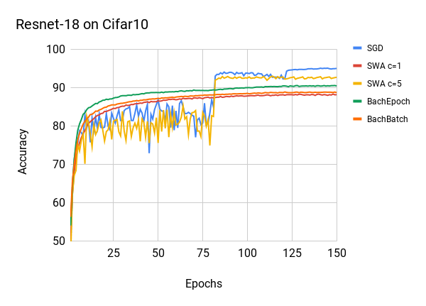
Figure 1: Performance of aforementioned algorithms  [20, 10].

From Figure 1, we see that none of the approaches can replicate the SGD accuracy. This trend is consistent across different models under optimal hyperparameter settings. When using the SWA technique in [20], the approaches deteriorate performance and hinder convergence. The performance improves with higher values of ‘c’ because of fewer reassignments of the SWA technique. [10] approach of using weighed averaging with more significance to later epochs in a linear (BachEpoch) and exponential (BachBatch) fashion also fail to converge optimally. All approaches add an increased computational load in processing of PRA for each model parameter while training, reassignment of the computed values, followed by recalibration of BN layers. These loads add up because all three tasks are performed for each epoch while training. Hence the techniques of  [20] and  [10] which work impressively over improving generalization of pretrained neural networks and optimizing convex learning models respectively, when translated to DNN training, increase the computational load and training time without providing optimal convergence.

3 Methods

3.1 PSWA

The analysis of the performance of the two methods shows that both SWA and weighed averaging do provide better generalization at the early stages of the training process, typically in the underfitting regime. However, as the mean is biased by the model weights at the early stages of the training process, it cannot converge properly at the later stages of the training, even when one allows weighted averaging in favor of models at later training stages. We address this problem by removing the dependency of any prior weight distribution estimations for the general PRA approach.

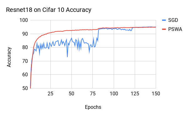
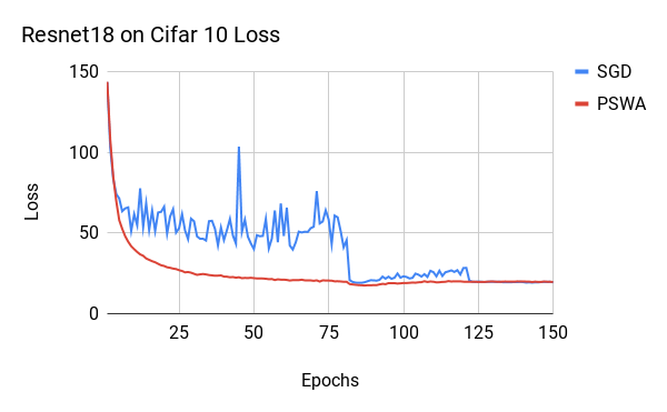
Figure 2: Performance of PSWA on test data during training.

We call this technique Periodically Sampled Weight Averaging (PSWA), as we sample the model weights over the batchwise updates, and repeat it periodically over each epoch. Figure 2 depicts the application of PSWA on ResNet18 for Cifar10 Accuracy and Cross Entropy Loss on the test dataset. We keep the experimental settings consistent with the prior experiments as well as for the experiments in following section, where we simply use SGD to refer to SGD with momentum and L2 weight penalty and consistent learning rate schedules unless otherwise mentioned. The details of our implementation can be found in the Experiments section. The approach allows the model to train effectively for one epoch, while keeping running means for all model parameters over the weight distribution after batchwise gradient updates, followed by reassigning the running mean to the parameter weights, and then reinitializing the mean at the end of the epoch. This additional step allows for SGD to gradually converge the model to the optimum by making gradient updates. Meanwhile, averaging over the batchwise distribution provides for a stabling effect on the model.

An important challenge for applying general weight averaging techniques for DNN models is the added computational load, which leads to longer training times. The time complexity of model training with weight averaging typically contains three parts:

$$T_{\text{total}}=T_{\text{backprop}}+\alpha T_{\text{weight update}}+\beta T_{\text{calibrate BN}},$$ (3)

where $T_{\text{backprop}}$, $T_{\text{weight update}}$, $T_{\text{calibrate BN}}$, mark the time spend on back-propagation, weight sampling, and Batch-Norm calibration using the full training dataset. Using the plain PSWA for the same number of epochs clearly leads to a longer training time.

1:

2:Initialize DNN model $\mathbf{w}^{(0)}$

3:Initialize Learning rate schedule $\eta(e)$

4:Initialize training data batches $D_{1}$ … $D_{b}$

5:Initialize total epochs $epochs$

6:Initialize running mean $\hat{\mathbf{w}}$ for $\mathbf{w}^{(0)}$ parameters

7:Determine sampling strategy and $\alpha,\beta$

8:

9:for  $e$ in 1 … $epochs$ do

10:     randomize($D_{1}$ … $D_{b}$)

11:     reset ($\hat{\mathbf{w}}$, 0)

12:     for  $i$ in 1 … $b$ do

13:         $\mathbf{w}^{(i)}=\mathbf{w}^{(i-1)}-\eta\nabla_{\mathbf{w}}l(\mathbf{w}^{(i)},D_{i})$

14:         update ($\hat{\mathbf{w}}$, $\mathbf{w}^{(i)}$, $i$, $\alpha$)      

15:     $\mathbf{w}^{(e)}$ . assign($\hat{\mathbf{w}}$)

16:     BN recalibration ($\beta$)

Algorithm 1 Periodically Sampled Weight Averaging

To remedy this additional computational load, we improve the plain-vanilla PSWA such that we update the running mean for only a few percent ($\alpha$) of the randomly selected batches spread evenly over the training data; Similarly, we recalibrate the global mean and variance of each BN layer with $\beta$ percent of the training data using a fast forward pass. We demonstrate later on that by reducing the number of updates in this fashion, the added computational cost becomes negligible for large datasets.

Algorithm 1 presents the general workflow of the PSWA method for training a DNN. After initializing the model parameters and data for training, we repeatedly update the model weights by SGD or other gradient-based optimizations. Then we update the mean estimation of each weight. The update is carried out in an online fashion. For $\alpha=100\%$ where we use the full dataset, it is:

$$\hat{w}\leftarrow\frac{i-1}{i}\hat{w}+\frac{w^{(i)}}{i}$$ (4)

To reduce the computational time, we only select $\alpha$ percent of batches to be used for mean estimation, and we change the count $i$ correspondingly. Before each epoch, we always reset the $\hat{w}$ to 0, and after the epoch, we reassign the mean weights to model weights. After reassigning, the BN layers are not best suitable for the new set of weights, so we recalibrate the BN layers using $\beta$ percent of the training data to perform a forward pass and recompute global mean and variance statistics for each BN layer.

3.2 PWALKS and PSWM

Although the PSWA method achieves optimal test accuracy using shallow ResNet18 model and other lightweight models, we found that for deeper networks PSWA still does not converge properly to the optimum. Figure 3 shows the effect on ResNet50. This problem is pervasive across similar deep networks like Inception and DenseNet, and also on datasets like ImageNet. However, it is important to note that the learning rate schedule decreases by a factor of 10 at epochs 80 and 120, and that it is only after the 120th epoch that the SGD method converges to a better result than PSWA.

To investigate why this happens, we analyze PSWA in more detail. In essence, for PSWA, we modify the algorithm of [10] which works over the entire training process, to run over only one epoch without any prior. This approach does not burden the running mean with the weights distribution of the earlier epochs while still providing regularizing effect from PRA over batchwise weight distribution. It however becomes cumbersome when the learning rate has decreased significantly as the batchwise descent of the SGD loss function is able to reach a deeper minima for more complex models. We believe that by performing PRA over the SGD walk at this stage, the regularization counteracts the optimal convergence to the minima at the latter part of the batch-wise training. To address this problem we return to the conclusions presented by [11], who show that there is a need to carefully remove from the running mean, the initial weights which bias the mean towards the local minima.

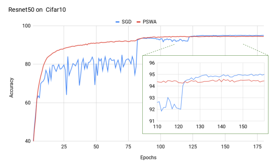
Figure 3: PSWA on ResNet50 convergence problem.

We solve the suboptimal convergence problem for deeper networks by proposing two different modifications to PSWA. In both approaches we allocate more importance to the model weights during the final batches while still maintaining the regularization afforded by using the weight distribution.

In the first approach, Periodic Weight Averaging over Last K Samples (PWALKS), instead of sampling weights evenly from all batches (for the mean weight distribution), we sample only the last ‘k’% of the samples, ‘k’ being a hyperparameter of size of the dataset and batches, ranging between 0 (last batch only, standard SGD) and $100$ (PSWA with $\alpha=1$). Empirically a small k value between 2-5 provides a consistently good performance by providing improvement over plain SGD during early training (though not as much as PSWA), and consistently converges to the optimum as demonstrated in Figure 4. Parallels can be drawn between the PWALKS technique and constructing an ensemble of models over the last few batches, however, we incorporate the modified weights as part of the training process iteratively, unlike ensemble models. To convert PSWA to PWALKS, the update (line 7) of Algorithm 1 is applied only when

$$i>b\times(1-k\%).$$ (5)

Moreover, the parameter k is equivalent to $\alpha$ in the PSWA method in terms of controlling computational cost.

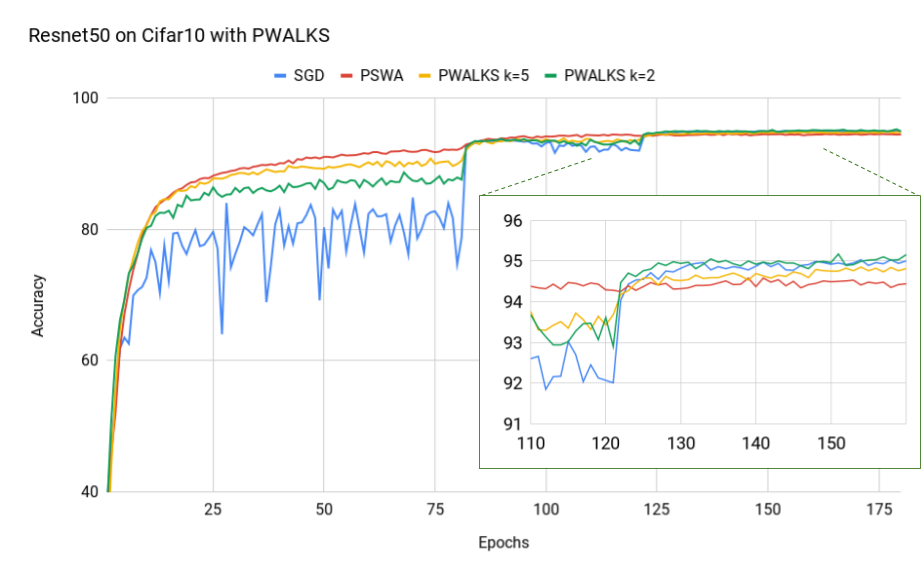
Figure 4: PWALKS comparisons.

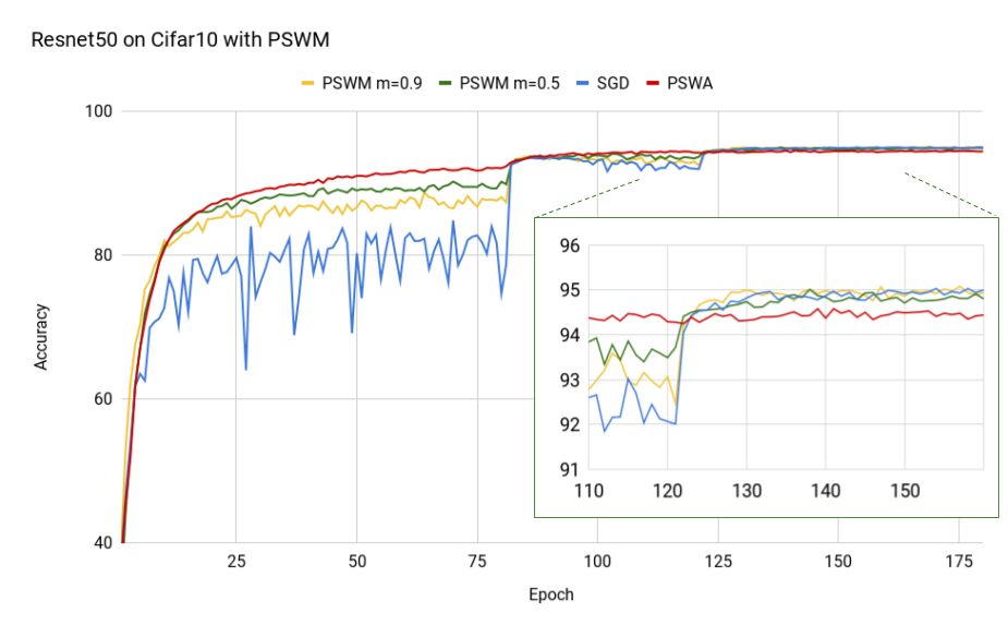
Figure 5: PSWM comparisons.

A second approach to solving the PSWA convergence problem is to approach it from the perspective of a cumulative adjustment to weights. We propose a momentum-based modification to PSWA called Periodically Sampled Weight Momentum (PSWM) where instead of keeping a running mean, we keep the running weights updated using momentum. For the model’s parameters we keep a running momentum term, which we update at the end of each batch and reassign at the end of the epoch. Empirically momentum values between (0.5,0.9) yield good performance with $m=1$ being standard SGD. To convert PSWA to PSWM, the update (line 7) of Algorithm 1 is changed to:

$$\hat{w}\leftarrow(1-m)\times\frac{i-1}{i}\hat{w}+m\times\frac{w^{(i)}}{i}.$$ (6)

And since the PSWM is built on the PSWA, the sampling technique developed for PSWA can be applied to also reduce the time complexity of PSWM.

We next compare the computational performances of plain-vanilla SGD, PSWA with $\alpha=\beta=1$ and PWALKS with $k=10$ and $\beta=10\%$. The code is based on the fastest Cifar10 training code listed in the DAWN project ([1]); and the original implementation is changed from half-precision to full precision. We repeated the training process 10 times for each technique and report the corresponding mean and standard deviations. Figure 6 shows that the PSWA leads to a 34% overhead when using the full training dataset for weight update and recalibration of BN layers; and by adopting PWALKS, we achieve the same prediction accuracy on the testing dataset without sacrificing the speed significantly without code-level optimizations, resulting in a 6% overhead on training time. In addition, we also observe that the variations of the training process is much smaller when weight averaging techniques have been applied, which we discuss in results section.

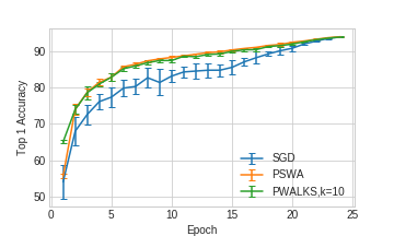
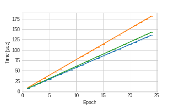
Figure 6: Comparison of computation time for plain-vanilla SGD, PSWA with $\alpha=1$ and PWALKS.

4 Experiments

We have already covered experiments on Cifar10 with Resnet18 and Resnet50 using our techniques with SGD. The experimental settings of the previous experiments use Momentum values of 0.9, L2 weight penalty of 5e-4, learning rate decays of 0.1 at epochs of 80 and 120, for a total of 150 epochs. These experiments were performed with tuned hyperparameters and learning rate schedules to ensure optimal convergence. We now explore how our methods translate to other datasets, models and optimizers.

4.1 Dataset: ImageNet

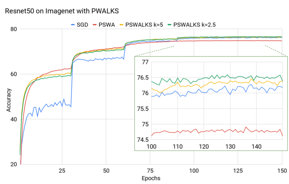
Figure 7: ResNet50 on ImageNet with PWALKS.

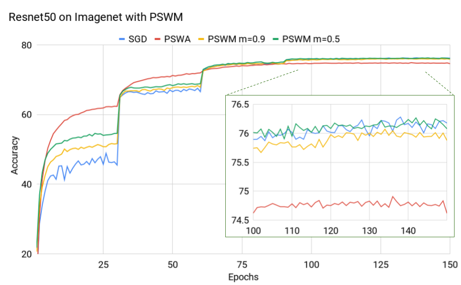
Figure 8: ResNet50 on ImageNet with PSWM.

ImageNet [2] is another standard image classification dataset, it has 1.2 million high resolution images from 1000 classes. Our implementations use ResNet50 as the underlying network, and SGD with momentum as the optimizer. We use learning rate with 0.1, which changes by a factor of 0.1 every 30 epochs, for a total of 150 epochs. Our results on ImageNet top-1 accuracy follow similar trends as on Cifar10 presented in Figure 7 and Figure 8 for PWALKS and PSWM respectively.

4.2 Optimizer: Adam

To show our techniques can be effectively used on adaptive optimizers as well, we present experiments on Adam  [8], which performs first-order gradient-based optimization of stochastic objective functions, based on adaptive estimates of lower-order moments. Figure 9 shows the implementation of ResNet50 on Cifar10 consistent with prior implementations except we use Adam instead of SGD, with a starting learning rate of 0.001. As we can see PSWA, PWALKS and PSWM all offer marginal but consistent improvement on Adam, across epochs over multiple runs. The improvement is not as significant and dramatic as SGD, because Adam itself alleviates the common problems of SGD like large fluctuations, and slow convergence. Since Adam modulates the learning rate of each weight based on the magnitudes of its gradients, instead of the complete raw and noisy gradient vector, the distribution of the parameter weights remains small compared to SGD.

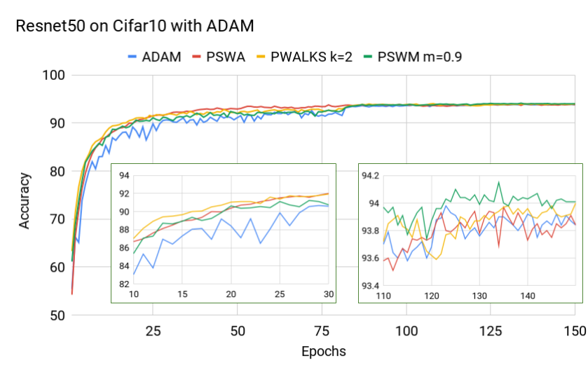
Figure 9: ResNet50 with Cifar10 using Adam.

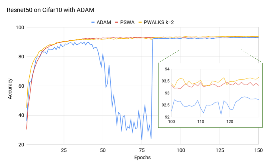
Figure 10: ResNet50 on Cifar10 with Adam and high learning rate.

Adam and other adaptive optimizers suffer from some important documented problems. Though Adam converges faster, it does not generalize well ([7]). From our experiments PSWA over Adam also provided for reduced CrossEntropy loss over training. Another problem for adaptive optimizers like RMSPROP and Adam is they become unstable at high learning rates near convergence. This happens as the squares of rolling mean of gradients are used to divide the current gradient, in which case very small gradients can introduce instability. In Figure 10 we present such a scenario where we use a $l$ of 0.01 (instead of 0.001) which causes Adam to become unstable. However, Adam with PSWA remains stable and converges better.

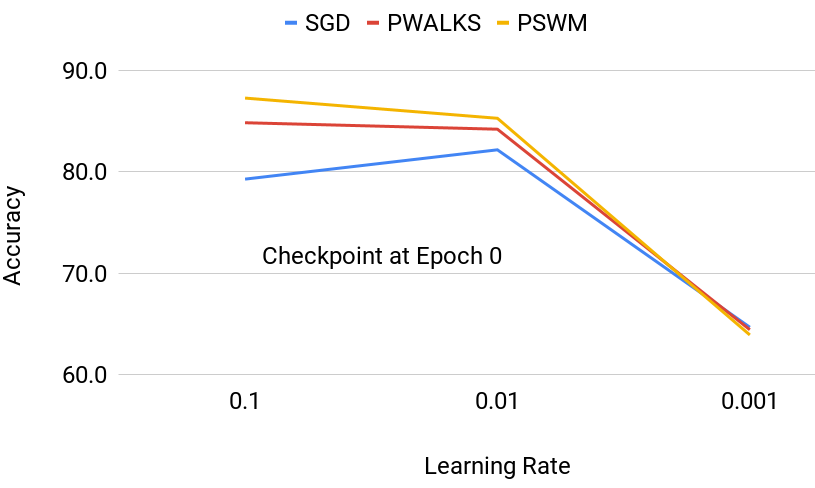
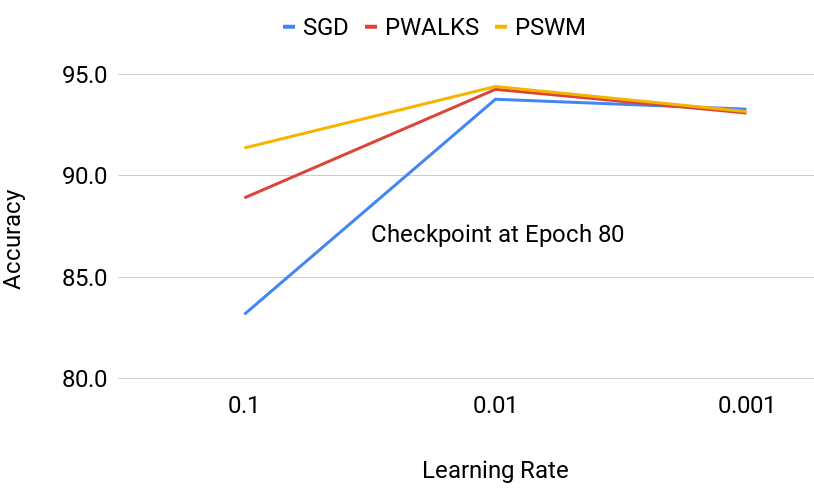
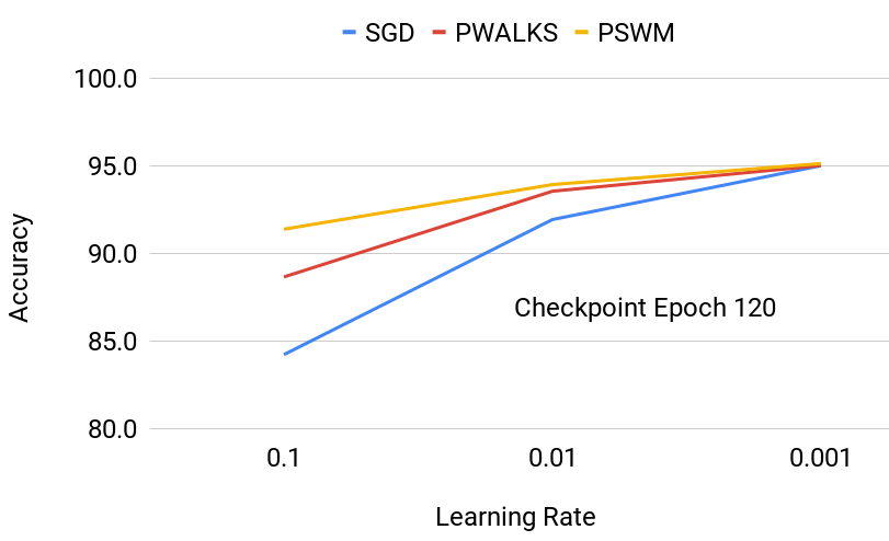
Figure 11: Faster convergence from different checkpoints and learning rates on Cifar10

4.3 Other Experiments

We perform more experiments using different model architectures like MobileNet [23], Inception [24], Densenet [19] which are presented in the supplementary paper along with experiments on Human Pose detection and Scene segmentation to cover a broad array of Computer Vision applications. We perform extensive experiments on Cifar10 under different configurations such as suboptimal learning rates and retraining from checkpoints, since these experiments are faster and their results generalize well to larger datasets like Imagenet. These experiments help analyze the strengths of our algorithms discussed in Results section.

5 Results

In this section we analyze the performance of our algorithms and try to quantify the improvements afforded by them. We use performance statistics of Resnet18 and Resnet50 on Cifar10 and Imagenet respectively, and compare PSWA, PWALKS (k=2), PSWM (m=0.5) against the baseline implementations which use SGD. We see for both Cifar10 and Imagenet, PSWA converges much faster during early training, but does not converge optimally. PWALKS provides better generalization than PSWM, while both the techniques provide improvement over SGD. Hence in this section we focus more on PWALKS, owing to its superior empirical performance. We show how our methods can provide faster, better and more robust performance empirically across different datasets, models and experimental settings. We note that since these terms have an overlap in their definitions, it is important how we interpret them in the the context of non-convex optimization and deep learning. Moreover, it is non-trivial to quantify this improvement as both the accuracy and loss functions form a non-stationary and volatile time-series.

5.1 Faster

We can interpret an algorithm being faster than a baseline approach if it achieves a performance threshold before the baseline. For our results we use validation thresholds of 90%, 95% for Cifar10; 92%, 93% [1] for top-5 and 75% for top-1 for Imagenet. These thresholds represent performance at near convergence and at convergence for the corresponding models and datasets, we present the results in Table 1. It is important to note that for Imagenet, PSWM and PWALKS cross the at convergence thresholds not only with fewer epochs compared to the baseline approach but with larger learning rates. SGD needs learning rate to decrease by a factor 0.1, under the same experimental settings to cross the thresholds.

Table 1: Epochs to achieve various accuracy thresholds.

	Baseline	PSWA	PSWM	PWALKS
Cifar10, 90%	81	22	22	64
Cifar10, 95%	137	N.A.	128	140
Imagenet (top 1) 75%	91	N.A.	72	80
Imagenet (top 5) 92%	69	83	66	65
Imagenet (top 5) 93%	129	N.A.	103	93

Another interpretation of faster can be in terms of convergence of the optimization algorithm for various stages and learning rates of the training process. We train Resnet18 on Cifar10 using the baseline SGD implementation and save checkpoints at epochs 0, 80, 120. We then retrain the checkpoints under different learning rates for 10 epochs and compare the results in Figure 11. As we can see, for all starting checkpoints, our algorithms converge much faster than baseline SGD at high and optimal learning rates. When the learning rate is very small, variances of the weight distributions are correspondingly small as well and hence our algorithms match the SGD performance.

5.2 Better

We emphasize that in all our presented examples, the optimizer, learning rate (and its schedule), and training hyperparameters, have all been finetuned for convergence for the original baseline implementations, and we do not modify them when using our techniques to ensure fair comparisons. But for most machine learning applications we are unaware of these optimal hyperparameters and learning rate schedules which can introduce volatility in the training process and uncertainty regarding the final convergence. We simulate these conditions on Cifar10 with Resnet18, while keeping the same experimental setting as before but with initial learning rates which are suboptimal. The results are presented in Table 2. As we can see when we have suboptimal training routines, we can still expect better performance and generalization from PSWM and PWALKS.

Table 2: Accuracy when training Resnet18 on Cifar10 with initial suboptimal learning rates. Optimal learning rate is 0.1

Algorithm	LR = 1	LR = 0.5	LR = 0.05	LR = 0.01
SGD	85.2	91.2	94.9	94.1
PWALKS	86.6	91.6	94.9	94.1
PSWM	88.0	91.6	95.2	94.1

Table 3: Intermediate accuracy improvement when training ResNet50 on ImageNet.

	Average Improvement over SGD accuracy for all epochs	Average Improvement over SGD accuracy for first 30 epochs
PSWA	2.75	12.52
PWALKS	3.50	12.37
PSWM	2.01	7.81

Since the baseline models are tuned to reach convergence, we can also analyze the intermediate performance during the training process under optimal experiment settings. We focus on intermediate performance both over the entire training process and during the early stages at high learning rates, presented in Table 3. These scenarios have direct applications in online learning and learning on resource constrained devices respectively, as presented in Discussions section. From these results it is clear that when we are dealing with suboptimal training settings our algorithms can provide better performance, and under optimal training settings we still provide better intermediate performance. We can also interpret Figure 11 in terms of better performance under different initial settings and learning rates.

5.3 Robust

We analyze the test accuracy distribution with ResNet50 over ImageNet and discover all three of our techniques provide consistent and significantly lower Standard Deviation (SD), both at convergence and over the saturation phases at constant learning rates as shown in Table 4. The lower variance at early saturation phase (epoch 20-30) points to a less volatile training process and the lower variance at the final 20 epochs point to a more stable convergence. Another important observation is that PWALKS and PSWA performance on the test set monotonically increases or remains stable over epochs until convergence. This is especially important since it indicates that with a high probability the model is consistently improving and the performance does not sporadically fluctuate like the baseline model. Again analyzing test accuracy distribution with ResNet50 over ImageNet, we find that for almost 70% consecutive epochs with PSWA the accuracy is improving, or 99% of them are stable within 0.2 percentage decrement, unlike SGD-based training which only shows 57% and 86% respectively (shown in Table 5). We also compare performance improvements between current epoch and best overall performance over previous epochs and present the stability within 0.2 percentage decrement. As we can see PSWA improves upon best previous performance or remains stable for 99% of the epochs.

Table 4: Volatility analysis of training ResNet50 on ImageNet.

	Standard Deviation last 20 epochs	Standard Deviation epochs 20-30	Mean last 20 epochs
SGD	0.080	1.06	76.16
PSWA	0.058	0.39	74.77
PWALKS	0.047	0.21	76.50
PSWM	0.056	0.24	76.16

Table 5: Monotonic improvement demonstrating stability when training ResNet50 on ImageNet. (% of epochs )

	improvement over previous	stable improvement over previous	stable improvement over max previous
SGD	57%	86%	77%
PSWA	70%	99%	99%
PWALKS	65%	98%	97%
PSWM	65%	96%	90%

6 Discussions and Additional Details

Following the Results section we see these advantages can significantly improve several computer vision based applications. Since PWALKS performs better at high learning rates (which offers training speed-up) and plateaus over shorter time, it can be especially useful when training on large datasets with constrained computational resources that require training at high learning rates for short time periods. These conditions arise for deep learning on Edge Devices where the models cannot realistically be trained to convergence. Moreover, PWALKS’ stability and monotonic improvements during training can uniquely benefit deployed models learning in an online fashion or over continuous streaming data, since PWALKS ensures models will not sporadically deteriorate during different phases of the training process.

Our analysis of the loss surface (presented in the supplementary paper) shows that these techniques produce minima that are deeper and wider than those found by SGD. The details of the implementations and system information necessary for reproducibility are also provided in supplementary paper along with other experiments. Also, while both PWALKS and PSWM offer optimal convergence, they depend on hyperparameters ‘k’ and ‘m’ respectively. Empirically we find that both techniques converge optimally to within a small margin to each other across a wide range of their respective hyperparameter values, and there isn’t an explicit need for researchers to tune them.

7 Conclusion

In this paper, we introduced a trio of techniques (PSWA, PWALKS, and PSWM) based on sampling over model weights that solve issues with previous weight averaging approaches. Our proposed techniques provide increased robustness and stability to the training process (Table 5) of neural networks as well as substantial intermediate performance improvements (Table 3) without compromising on optimal convergence (Table 4). PWALKS’ almost monotonic and stable performance (Table 5) ensures performance does not fluctuate depending on the current batch. As (Table 1) reflects, our techniques can provide faster convergence for thresholds and for different checkpoints under diverse experimental settings (Figure 11). In the light of the advantages offered by these techniques, they provide a good starting point for training DNNs especially in those cases where no optimal training regime exists.

Supplementary Material

	Stochastic Gradient Descent	PSWA (with SGD)
	Initialize:  $\boldsymbol{w}^{1,0}\leftarrow 0$	$\boldsymbol{w}^{1,0}\leftarrow 0$
Epoch 1	$\begin{aligned} \boldsymbol{w}^{1,1}\leftarrow\boldsymbol{w}^{1,0}-\eta\times\boldsymbol{g}^{1,0}\\ \boldsymbol{w}^{1,2}\leftarrow\boldsymbol{w}^{1,1}-\eta\times\boldsymbol{g}^{1,1}\\ \vdots\\ \boldsymbol{w}^{1,T}\leftarrow\boldsymbol{w}^{1,T-1}-\eta\times\boldsymbol{g}^{1,T-1}\end{aligned}$	$\begin{aligned} \boldsymbol{w}^{1,1}\leftarrow\boldsymbol{w}^{1,0}-\eta\times\boldsymbol{g}^{1,0}\\ \boldsymbol{w}^{1,2}\leftarrow\boldsymbol{w}^{1,1}-\eta\times\boldsymbol{g}^{1,1}\\ \vdots\\ \boldsymbol{w}^{1,T}\leftarrow\boldsymbol{w}^{1,T-1}-\eta\times\boldsymbol{g}^{1,T-1}\\ \end{aligned}$
	Initialize:  $\boldsymbol{w}^{2,0}\leftarrow\boldsymbol{w}^{1,T}$	$\boldsymbol{w}^{2,0}\leftarrow\frac{1}{T}\sum_{t=1}^{t=T}\boldsymbol{w}^{1,t}$
Epoch 2	$\begin{aligned} \boldsymbol{w}^{2,1}\leftarrow\boldsymbol{w}^{2,0}-\eta\times\boldsymbol{g}^{2,0}\\ \boldsymbol{w}^{2,2}\leftarrow\boldsymbol{w}^{2,1}-\eta\times\boldsymbol{g}^{2,1}\\ \vdots\\ \boldsymbol{w}^{2,T}\leftarrow\boldsymbol{w}^{2,T-1}-\eta\times\boldsymbol{g}^{2,T-1}\\ \end{aligned}$	$\begin{aligned} \boldsymbol{w}^{2,1}\leftarrow\boldsymbol{w}^{2,0}-\eta\times\boldsymbol{g}^{2,0}\\ \boldsymbol{w}^{2,2}\leftarrow\boldsymbol{w}^{2,1}-\eta\times\boldsymbol{g}^{2,1}\\ \vdots\\ \boldsymbol{w}^{2,T}\leftarrow\boldsymbol{w}^{2,T-1}-\eta\times\boldsymbol{g}^{2,T-1}\\ \end{aligned}$
	⋮	⋮
Epoch E	$\begin{aligned} \text{\text@underline{Initialize:}}\quad\boldsymbol{w}^{E,0}\leftarrow\boldsymbol{w}^{E-1,T}\\ \boldsymbol{w}^{E,1}\leftarrow\boldsymbol{w}^{E,0}-\eta\times\boldsymbol{g}^{E,0}\\ \boldsymbol{w}^{E,2}\leftarrow\boldsymbol{w}^{E,1}-\eta\times\boldsymbol{g}^{E,1}\\ \vdots\\ \boldsymbol{w}^{E,T}\leftarrow\boldsymbol{w}^{E,T-1}-\eta\times\boldsymbol{g}^{E,T-1}\\ \boldsymbol{w}^{Final}\leftarrow\boldsymbol{w}^{E,T}\\ \end{aligned}$	$\begin{aligned} \boldsymbol{w}^{E,0}\leftarrow\frac{1}{T}\sum_{t=1}^{t=T}\boldsymbol{w}^{E-1,t}\\ \boldsymbol{w}^{E,1}\leftarrow\boldsymbol{w}^{E,0}-\eta\times\boldsymbol{g}^{E,0}\\ \boldsymbol{w}^{E,2}\leftarrow\boldsymbol{w}^{E,1}-\eta\times\boldsymbol{g}^{E,1}\\ \vdots\\ \boldsymbol{w}^{E,T}\leftarrow\boldsymbol{w}^{E,T-1}-\eta\times\boldsymbol{g}^{E,T-1}\\ \boldsymbol{w}^{Final}\leftarrow\frac{1}{T}\sum_{t=1}^{t=T}\boldsymbol{w}^{E,t}\\ \end{aligned}$

Table 6: Standard SGD and PSWA algorithm updates for E epochs (with T iterations per epoch).

8 Motivation

Our motivation for intermediate averaging stems from the stability induced into the standard SGD updates through various averaging schemes [27]. We illustrate this by comparing the standard SGD with the periodically sampled weight averaging (PSWA). The layout of the updates for $E$ epochs (with $T$ iterations per epoch) for the algorithms is provided in Table 6. Here we define, $\boldsymbol{w}^{e,t}$ = model weights during the $e^{th}$ epoch and $t^{th}$ iteration within an epoch, with $t=0\ldots T$ and, $e=0\ldots E$ . For simplicity we fix the batch size for SGD updates to 1. Further, $\eta$ is the constant learning rate, and at each step an oracle provides with the vector $\mathbb{E}(\boldsymbol{g}^{e,t})\in\partial f(\boldsymbol{w}^{e,t})$, where $\mathop{\mathbb{E}}$ is the expectation operator. Finally, we use $\boldsymbol{w}^{\ast}$ as the model weights at convergence.

Next, we define a notion of stability which simply captures the variance of the expected function values at the end of each epoch from convergence.

Definition 1.

Stability of an algorithm $\mathcal{A}$ is defined as

$$\mathcal{S}_{\mathcal{A}}=\|\boldsymbol{s}^{\mathcal{A}}\|^{2}_{2}$$

where

$$\boldsymbol{s}^{\mathcal{A}}=[\,\boldsymbol{s}^{\mathcal{A}}_{1}...\boldsymbol{s}^{\mathcal{A}}_{e}...\boldsymbol{s}^{\mathcal{A}}_{E}]\;\forall e=1\ldots E$$

and

$$\boldsymbol{s}_{e}^{\mathcal{A}}=\mathop{\mathbb{E}}(f(\boldsymbol{w}_{e}^{\mathcal{A}})-f(\boldsymbol{w}^{\ast}))$$

From this definition it is clear that it is desirable to have smaller $\mathcal{S}_{\mathcal{A}}$ for more stable algorithms.

Next, to analyze the stability of the standard SGD and the PSWA method, we use the Theorems 1 and 2 respectively, presented next. Theorem 1 provide the best provable convergence rate for standard SGD with the following assumptions,

Assumption 1.

We make the minimal assumptions,

1. The function $f$ is convex in $\boldsymbol{w}$ with convex domain $\mathcal{W}$.

2. Bounded difference i.e. there exists a constant $D=\underset{\boldsymbol{w},\boldsymbol{w}^{\prime}\in\mathcal{W}}{sup}||\boldsymbol{w}-\boldsymbol{w}^{\prime}||_{2}^{2}$ with $D<\infty$.

3. Bounded gradients i.e. $\mathbb{E}(||\mathbf{g}^{e,t})||_{2}^{2}\leq G^{2}$.

Note that here although our analysis assumes a convex function, we make mild assumptions on the nature (stability) of the functions. Under Assumption 1 we have the following,

Theorem 1.

Under Assumption 1 the standard SGD algorithm after $e$ epochs (with $T$ iterations per epoch) with a step size $\eta_{t}=1/\sqrt{t}$,   $t=1\ldots Te$ provides,

$$\mathop{\mathbb{E}}[\,f(\boldsymbol{w}_{e,0}^{SGD})-f(\boldsymbol{w}^{\ast})]\leq(D^{2}+G^{2})\frac{2+log(T(e-1))}{\sqrt{T(e-1)}}$$

$$\quad\quad\quad\quad\quad\quad\quad\quad\quad\quad\simeq\;\mathbb{O}(\,\frac{\log(Te)}{\sqrt{Te}})$$

Proof: The proof follows by direct application of Theorem 2 in [27] for T(e-1) iterations. ∎

In fact, under the similar assumptions we see that the PSWA algorithm follows,

Theorem 2.

Under Assumption 1 the PSWA algorithm after $E$ epochs (with $T$ iterations per epoch) and a constant step size $\eta=\sqrt{\frac{D^{2}}{TG^{2}}}$ provides,

$$\mathop{\mathbb{E}}[\,f(\boldsymbol{w}_{e,0}^{PSWA})-f(\boldsymbol{w}^{\ast})]\leq\frac{(DG)}{\sqrt{T}}\simeq\;\mathbb{O}(\,\frac{1}{\sqrt{T}})$$

Proof: The proof follows through applying Theorem 14.8 in [28] for the final epoch $E-1$ of PSWA and bounding $||\boldsymbol{w}^{e-1,0}-\boldsymbol{w}^{*}||_{2}^{2}\leq D^{2}$. ∎

Remark A straight-forward comparison from Theorems 1 & 2 and using the Definition 1 shows that, for sufficiently large $T\gg e$, the PSWA has better stability i.e. $\boldsymbol{s}_{e}^{\text{PSWA}}\simeq\mathbb{O}(\,\frac{1}{\sqrt{T}})\leq\mathbb{O}(\,\frac{\log(Te)}{\sqrt{Te}})\simeq\boldsymbol{s}_{e}^{\text{SGD}}$. This indicates through periodically sampling we can improve the stability of the algorithm at least in the initial stages of the algorithm where $T\gg e$. This intuition is further validated through our Experiments in Section 3 of the main paper.

9 Additional Experiments

9.1 Dataset: Cifar10

We have already discussed in detail the results of our techniques on ResNet18 and ResNet50 over Cifar10. ResNet18 is trained for 150 epochs and ResNet50 is trained for 180 epochs. Both use SGD with momentum of 0.9, L2 penalty of 0.0005, and have a learning rate schedule which decreases by factor of 10 at epochs 80,120 and 150. We use Standard CrossEntropy loss and batch size of 128.

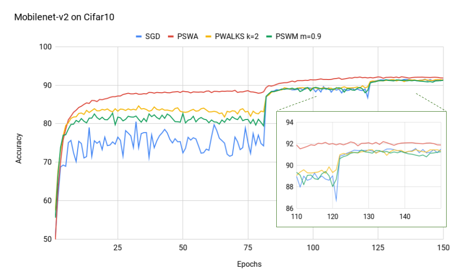
Figure 12: MobileNet trained on Cifar10.

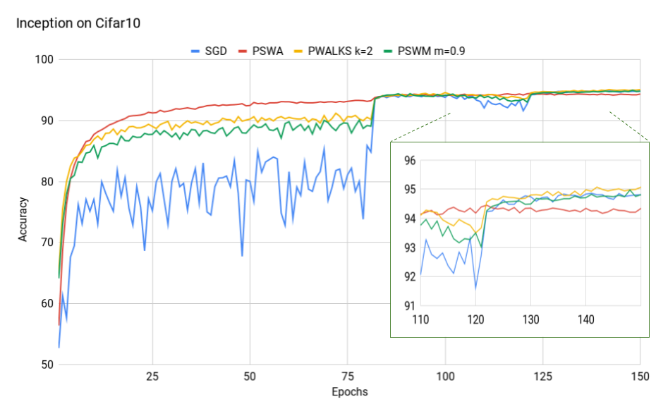
Figure 13: Inception trained on Cifar10.

In our experiments on shallow networks like MobileNet-v2 [23] and ResNet18, we find PSWA not only provides faster and more robust convergence, but also converges to a more optimal minima, as evident in Figure 12. Another interesting comparison is between PWALKS and PSWM with PSWA on shallow networks, where PSWA converges to deeper minima, which PWALKS and PSWM are unable to. However, for deeper networks like Inception [24] , DenseNet-121 [19] and ResNet50, as discussed before, PSWA does not converge properly, while both PWALKS and PSWM do. Figure 13 shows Inception network trained using the same implementation as above. We observe that PSWA and its variations reach 90% and 94% thresholds much faster consistently and while training on larger learning rate, while SGD needs a learning rate change by a factor of 10, to cross the thresholds.

9.2 Task: Human-Pose Detection

We apply our techniques on the work of [30], where they perform Human-keypoint detection on MS-COCO [29] and Human-pose detection on MPII dataset [31] . Both tasks use ResNet50 pretrained on ImageNet, and perform transfer learning on the new dataset. Both experiments use Adam as the optimizer with a learning rate of 0.001. Consistent with our prior experiments, PWALKS and PSWM provide consistent improvement over Adam in the early stages of training.

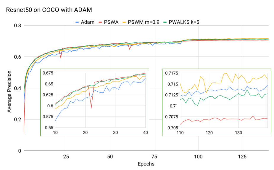
Figure 14: COCO-Keypoint detection on ResNet50 and Adam

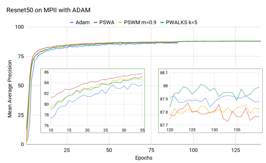
Figure 15: MPII Human-Pose detection on ResNet50 and Adam

9.3 Task: Segmentation

We also apply our techniques on the works of [33], where they perform scene segmentation on MIT ADE20K Dataset [35], the largest open source dataset for semantic segmentation and scene parsing. The implementation uses an encoder-decoder architecture with ResNet50 pretrained on ImageNet as the encoder and Pyramid Pooling Module with Bilinear Upsampling as decoder with deep supervision [32]. The implementation uses per-pixel cross-entropy loss, SGD as the optimizer and a ’poly’ learning rate policy.

For our implementation we initialize two distributions one each for the encoder and decoder. We update both the distributions together and reassign at the end of the epoch. We do not need to recalibrate the BN layers, since the implementation uses Synchronized Batch Normalization [34]. Figure 16 shows Pixel wise accuracy of the Segmentation models on test set and Figure 17 shows Mean IOU of the predicted segmentation on test data, where PSWA provides significant improvement over SGD based training.

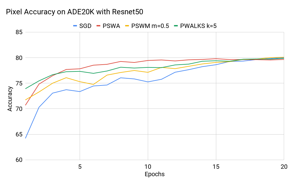
Figure 16: Pixel accuracy of segmentation on ADE20K.

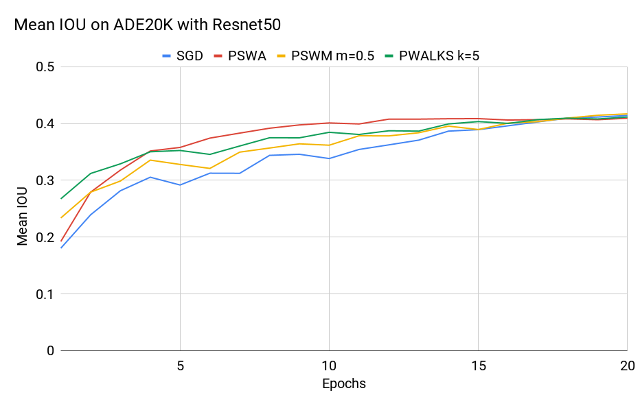
Figure 17: Mean IOU of segmentation on ADE20K.

10 Reproducibility

We provide details of hyperparameter values and additional implementation details about Experiments section.

For the experiments on Cifar10 We adopted the implementation in (https://github.com/kuangliu/pytorch-cifar/blob/master/main.py) with the exception of a custom learning rate schedule as the original was sub-optimal. Data augmentation on the training set was performed using random crop (padding 4) and horizontal flip while both train and test were normalized. The dataloaders perform random shuffle on data batches, with 2 concurrent workers for each test and train data queue. The code runs on Pytorch 1.0, Python 3.6, CUDA 9.0 with cuDNN. We use 1 Tesla V100 with 16 GB GPU memory and 8vCPU Intel Skylake.

For experiments on ImageNet We used the implementation in (https://github.com/pytorch/examples/tree/master/imagenet). We used a batch size of 32, L2 penalty of 0.0001, momentum of 0.9, and perform standard data augmentation like cropping, horizontal flipping and input data normalization. The code runs on Pytorch 1.0, Python 3.6, CUDA 9.0 with cuDNN. We use 4 Tesla V100 with 64 GB GPU memory and 32vCPU Intel Skylake.

For experiments on human pose estimation We adopted the implementation in
(https://github.com/Microsoft/human-pose-estimation.pytorch) . The code runs on Pytorch 1.0, Python 3.6, CUDA 9.0 with CudNN. We use 4 Tesla V100 with 64 GB GPU memory and 32vCPU Intel Skylake.

For semantic segmentation experiments We used
(https://github.com/CSAILVision/semantic-segmentation-pytorch) for implementation details. The code runs on Pytorch 1.0, Python 3.6, CUDA 9.0 with cuDNN. We use 4 Tesla V100 with 64 GB GPU memory and 32vCPU Intel Skylake.

11 Loss Surface Analysis

Model	Epoch 20	Epoch 100	Epoch 150
	(Early Training)	(Near Convergence)	(At convergence)
SGD
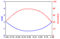
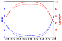
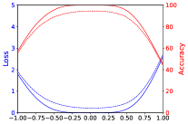
SGD + PSWA

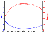
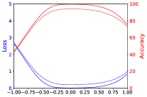
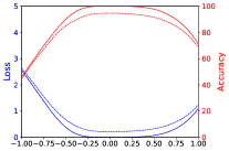
Figure 18: Comparison of loss surface with SGD and PSWA at different training stages.

To better understand the results of our approach, we investigate the effect of PSWA on the loss surface of the model during training when compared to SGD. Training neural networks requires minimizing a high-dimensional non-convex loss function, with a deeper minima correlating with better performance. An important characteristic of the minima is its ‘flatness’ or the measure of size of the connected region around the minimum where the training loss remains low. There exist strong claims that “flat” minima generalize better, while increased sharpness of a minima could indicate low generalization ([18, 21]). [20] shows their technique, SWA (based on averaging multiple points along the trajectory of SGD) leads to solutions corresponding to wider optima than SGD. We draw similar conclusions for PSWA.

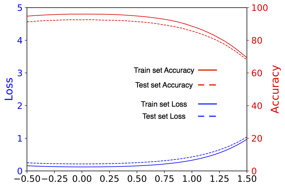
Figure 19: Loss surface of model weights before and after applying PSWA on one epoch.

We follow [22] approach, which presents a technique that calculates and visualizes the loss surface along random direction(s) near the weight space. They use a novel “filter normalization” scheme that enables side-by-side comparisons of different minima, which addresses problems with 1-Dimensional Linear Interpolation. Figure 18 presents loss surface comparison at different stages of training- beginning, near convergence, and at convergence on ResNet18 for Cifar10 trained by SGD and SGD with PSWA. The horizontal axis represents the displacement of the random Gaussian direction vector; the red lines indicate accuracy and the blue lines indicate the loss values; the dashed lines represent the values on the test dataset while the solid lines represent the training set. As is clearly evident, the model trained by PSWA has much flatter and deeper minima, for both training and testing set, at the early training stage. The trend continues for near convergence stage and at convergence, though it becomes less pronounced. We can see that with similar test and train accuracies, PSWA still retains wider minima. Figure 19 presents a different representation of the loss surface at early training stage (epoch 50), before and after reassigning the model weights. The PSWA-based model is located at index 0 on the horizontal axis, and SGD model at index 1, while variables between them represent the displacement in the “filter normalized” direction between the weights (since we use the same model). We notice steady improvements in performance in the direction of weights after PSWA is applied.

References

- [1] Cody Coleman, Deepak Narayanan, Daniel Kang, Tian Zhao, Jian Zhang, Luigi Nardi, Peter Bailis, Kunle Olukotun, Chris Ré, and Matei Zaharia. 2017. DAWNBench: An End-to-End Deep Learning Benchmark and Competition. NIPS ML Systems Workshop (2017).
- [2] Olga Russakovsky, Jia Deng, Hao Su, Jonathan Krause, Sanjeev Satheesh, Sean Ma, Zhiheng Huang, Andrej Karpathy, Aditya Khosla, Michael Bernstein, Alexander C. Berg, and Li Fei-Fei. 2015. ImageNet Large Scale Visual Recognition Challenge. In International Journal of Computer Vision (IJCV) 115(2015), 211–252.
- [3] John Duchi, Elad Hazan, and Yoram Singer. 2011. Adaptive subgradient methods for online learning and stochastic optimization. The Journal of Machine Learning Research 12, Jul (2011), 2121–2159.
- [4] Kaiming He, Xiangyu Zhang, Shaoqing Ren, and Jian Sun. 2016. Deep residual learning for image recognition. In Proceedings of the IEEE conference on computer vision and pattern recognition. 770–778.
- [5] Sergey Ioffe and Christian Szegedy. 2015. Batch normalization: Accelerating deep network training by reducing internal covariate shift. arXiv preprint arXiv:1502.03167 (2015).
- [6] Pavel Izmailov, Dmitrii Podoprikhin, Timur Garipov, Dmitry Vetrov, and Andrew Gordon Wilson. 2018. Averaging Weights Leads to Wider Optima and Better Generalization. (Mar 2018). https://doi.org/arXiv:1803.05407
- [7] Nitish Shirish Keskar and Richard Socher. 2017. Improving generalization performance by switching from adam to sgd. preprint arXiv:1712.07628 (2017).
- [8] Diederik P. Kingma and Jimmy Lei Ba. 2015. Adam: a Method for Stochastic Optimization. In International Conference on Learning Representations.
- [9] Alex Krizhevsky. 2009. Learning multiple layers of features from tiny images. Technical Report. Citeseer.
- [10] S. Lacoste-Julien, M. Schmidt, and F. Bach. 2012. A simpler approach to obtaining an O(1/t) convergence rate for the projected stochastic subgradient method. ArXiv e-prints (Dec. 2012). arXiv:1212.2002
- [11] Eric Moulines and Francis R. Bach. 2011. Non-Asymptotic Analysis of Stochastic Approximation Algorithms for Machine Learning. In Advances in Neural Information Processing Systems 24, J. Shawe-Taylor, R. S. Zemel, P. L. Bartlett, F. Pereira, and K. Q. Weinberger (Eds.). Curran Associates, Inc., 451–459.
- [12] Samuel L Smith, Pieter-Jan Kindermans, Chris Ying, and Quoc V Le. 2017. Don’t decay the learning rate, increase the batch size. preprint arXiv:1711.00489 (2017).
- [13] Tijmen Tieleman and Geoffrey Hinton. 2012. Lecture 6.5-rmsprop: Divide the gradient by a running average of its recent magnitude. COURSERA: Neural networks for machine learning 4, 2 (2012), 26–31.
- [14] Jiayi Liu, Samarth Tripathi, Unmesh Kurup, and Mohak Shah . 2018. Make (nearly) every neural network better: Generating neural network ensembles by weight parameter resampling. In arXiv preprint arXiv:1807.00847 (2018)..
- [15] Mark Sandler, Andrew Howard, Menglong Zhu, Andrey Zhmoginov, and Liang-Chieh Chen. 2018. MobileNetV2: Inverted Residuals and Linear Bottlenecks. In Proceedings of the IEEE Conference on Computer Vision and Pattern Recognition. 4510–4520.
- [16] Gao Huang, Zhuang Liu, Laurens Van Der Maaten, and Kilian Q Weinberger. 2017. Densely Connected Convolutional Networks.. In CVPR, Vol. 1. 3.
- [17] Christian Szegedy, Vincent Vanhoucke, Sergey Ioffe, Jon Shlens, and Zbigniew Wojna. 2016. Rethinking the inception architecture for computer vision. In Proceedings of the IEEE conference on computer vision and pattern recognition. 2818–2826.
- [18] Sepp Hochreiter and J Schmidhuber. 1997. Flat minima. Neural Computation 9, 1 (1997), 1–42.
- [19] Gao Huang, Zhuang Liu, Laurens Van Der Maaten, and Kilian Q Weinberger. 2017. Densely Connected Convolutional Networks.. In CVPR, Vol. 1. 3.
- [20] Pavel Izmailov, Dmitrii Podoprikhin, Timur Garipov, Dmitry Vetrov, and Andrew Gordon Wilson. 2018. Averaging Weights Leads to Wider Optima and Better Generalization. (Mar 2018). https://doi.org/arXiv:1803.05407
- [21] Kenji Kawaguchi. 2016. Deep learning without poor local minima. In Advances in Neural Information Processing Systems. 586–594.
- [22] Hao Li, Zheng Xu, Gavin Taylor, and Tom Goldstein. 2017. Visualizing the loss landscape of neural nets. arXiv preprint arXiv:1712.09913 (2017).
- [23] Mark Sandler, Andrew Howard, Menglong Zhu, Andrey Zhmoginov, and Liang-Chieh Chen. 2018. MobileNetV2: Inverted Residuals and Linear Bottlenecks. In Proceedings of the IEEE Conference on Computer Vision and Pattern Recognition. 4510–4520.
- [24] Christian Szegedy, Vincent Vanhoucke, Sergey Ioffe, Jon Shlens, and Zbigniew Wojna. 2016. Rethinking the inception architecture for computer vision. In Proceedings of the IEEE conference on computer vision and pattern recognition. 2818–2826.
- [25] Ohad Shamir, and Tong Zhang. 2013. Stochastic gradient descent for non-smooth optimization: Convergence results and optimal averaging schemes. In International Conference on Machine Learning 71–79.
- [26] Shai Shalev-Shwartz, and Shai Ben-David. 2014. Stochastic gradient descent. In Understanding machine learning: From theory to algorithms Cambridge university press, 184–201.
- [27] Ohad Shamir, and Tong Zhang. 2013. Stochastic gradient descent for non-smooth optimization: Convergence results and optimal averaging schemes. In International Conference on Machine Learning 71–79.
- [28] Shai Shalev-Shwartz, and Shai Ben-David. 2014. Stochastic gradient descent. In Understanding machine learning: From theory to algorithms Cambridge university press, 184–201.
- [29] Tsung-Yi Lin, Michael Maire, Serge Belongie, James Hays, Pietro Perona, Deva Ramanan, Piotr Dollár, and C Lawrence Zitnick. 2014. Microsoft coco: Common objects in context. In European conference on computer vision. Springer.
- [30] Bin Xiao, Haiping Wu, and Yichen Wei. 2018b. Simple Baselines for Human Pose Estimation and Tracking. arXiv preprint arXiv:1804.06208 (2018).
- [31] Mykhaylo Andriluka, Leonid Pishchulin, Peter Gehler, and Bernt Schiele. 2014. 2D Human Pose Estimation: New Benchmark and State of the Art Analysis. In IEEE Conference on Computer Vision and Pattern Recognition (CVPR).
- [32] Tete Xiao, Yingcheng Liu, Bolei Zhou, Yuning Jiang, and Jian Sun. 2018a. Unified Perceptual Parsing for Scene Understanding. preprint arXiv:1807.10221 (2018).
- [33] Bolei Zhou, Hang Zhao, Xavier Puig, Sanja Fidler, Adela Barriuso, and Antonio Torralba. 2017. Scene parsing through ade20k dataset. In Proceedings of the IEEE Conference on Computer Vision and Pattern Recognition, Vol. 1. IEEE, 4.
- [34] Chao Peng, Tete Xiao, Zeming Li, Yuning Jiang, Xiangyu Zhang, Kai Jia, Gang Yu, and Jian Sun. 2017. Megdet: A large mini-batch object detector. arXiv preprint arXiv:1711.07240 7 (2017).
- [35] Bolei Zhou, Hang Zhao, Xavier Puig, Sanja Fidler, Adela Barriuso, and Antonio Torralba. 2016. Semantic understanding of scenes through the ADE20K dataset. arXiv preprint arXiv:1608.05442 (2016).