Deep Neural Network Classifier for Variable Stars with Novelty Detection Capability

Abstract

Common variable star classifiers are built only with the goal of producing the correct class labels, leaving much of the multi-task capability of deep neural networks unexplored. We present a periodic light curve classifier that combines a recurrent neural network autoencoder for unsupervised feature extraction and a dual-purpose estimation network for supervised classification and novelty detection. The estimation network optimizes a Gaussian mixture model in the reduced-dimension feature space, where each Gaussian component corresponds to a variable class. An estimation network with a basic structure of a single hidden layer attains a cross-validation classification accuracy of $\sim 99\%$, on par with the conventional workhorses, random forest classifiers. With the addition of photometric features, the network is capable of detecting previously unseen types of variability with precision 0.90, recall 0.96, and an $F_{1}$ score of 0.93. The simultaneous training of the autoencoder and estimation network is found to be mutually beneficial, resulting in faster autoencoder convergence, and superior classification and novelty detection performance. The estimation network also delivers adequate results even when optimized with pre-trained autoencoder features, suggesting that it can readily extend existing classifiers to provide added novelty detection capabilities.

1 Introduction

Efficient classification of the variability of astrophysical objects is crucial to defining follow-up observations and analysis. With the advent of the next-generation surveys such as the Large Synoptic Survey Telescope (LSST, Ivezić et al., 2008; LSST Science Collaboration et al., 2009) and the Zwicky Transient Facility (ZTF Bellm et al., 2019), automatic pipelines are required to categorize an unprecedented amount of light curves into known or previously unseen variability classes. To this end, machine learning has been applied to solve the classification problem sufficiently. The identification of objects with novel variability properties, however, still relies heavily on visual inspection by human experts.

Classifiers are seldom trained using raw light curves due to their high and non-uniform number of observational epochs. Instead, ‘features’ of much lower dimensions are obtained, a process known as feature extraction. Features typically include the variable period (Lomb, 1976; Scargle, 1982; Schwarzenberg-Czerny, 1996; Kovács et al., 2002), amplitudes and ratios of different Fourier components (Nun et al., 2015), and summary statistics of the flux variation (e.g. standard deviation and skewness). Random forest (RF) classifiers trained on features obtained from photometric data have been the blueprint of most recent classification efforts (Richards et al., 2011; Dubath et al., 2011; Bloom et al., 2012; Kim et al., 2014; Masci et al., 2014; Kim & Bailer-Jones, 2016; Jayasinghe et al., 2018; Rimoldini et al., 2018). The new probabilistic RF method, which takes into account uncertainties in both features and labels (Reis et al., 2019), holds promise in improving RF’s performance. However, manual selection of features still requires tremendous human involvement.

Deep artificial neural networks have attracted recent attention in the physical sciences due to their ability to acquire meaningful data representations with minimal human input. In astrophysics alone, galaxy morphology classification (Dieleman et al., 2015; Aniyan & Thorat, 2017), transient and exo-planet detection (Cabrera-Vives et al., 2017; Shallue & Vanderburg, 2018; Sedaghat & Mahabal, 2018), and, of course, light curve classification (Aguirre et al., 2019; Muthukrishna et al., 2019) have benefited from the success of convolutional neural networks (CNNs) in image and sequential data processing.

Autoencoding recurrent neural networks (RNNs), which preserve the sequential information of input data, were found to be effective in extracting representative features from light curves (Naul et al., 2018). The encoder component of the network takes light curves as inputs and generates features of much lower dimension. The decoder then attempts to reconstruct the light curves using only the encoder-generated features. By matching the reconstructed light curves with the original inputs, the autoencoder learns to isolate essential features that characterize the light curves. Unlike the conventional approach where frequency and statistical features are hand-selected, the RNNs perform feature extraction without human intervention.

Most of the previous attempts at light curve classification focused only on correctly providing object labels. In a realistic workflow, however, an indispensable task is to uncover objects with previously unseen types of variability, so called novelty detection, among a large number of objects of known classes. Zong et al. (2018) have recently proposed a framework that combines autoencoding feature extraction with a Gaussian Mixture Model (GMM)-based unsupervised anomaly detection scheme.

In this letter, we present a neural network architecture that combines the efforts of Naul et al. (2018) and Zong et al. (2018). Namely, we jointly optimize an autoencoding RNN for feature extraction from variable light curves and an estimation network for classification and novelty detection. The motivation for this work is to promote the application of multi-task neural networks in variability analysis.

Figure 1: Schematic diagram of the neural network architecture. The structure of the RNN autoencoder follows Naul et al. (2018). The estimation network is similar to that used in Zong et al. (2018) except for the added one-hot conversion for the classification task.

2 Methods

2.1 Data and data pre-processing

The network is trained using the light curves from the All-Sky Automated Survey for Supernovae (ASAS-SN) Variable Stars Database I and II (Shappee et al., 2014; Jayasinghe et al., 2018). The light curves, obtained from the online database, typically have hundreds of epochs in V and g bands. From the vast database, only light curves of types listed in Table 1 were selected for classification purposes. These variability types will be referred to as the variable superclasses.

The data selection and pre-processing procedure closely resembles that of Naul et al. (2018). To minimize confusion, we selected sources based on information from the ASAS-SN variable star catalog. Classifications in the catalog, generated using their RF classifier, are treated as the true labels of the sources. We note that these labels may not be completely genuine. Only variables with classification probabilities above 90% and at least 200 epochs were used. Light curves with SuperSmoother residuals greater than 0.7 were omitted to ensure only true periodic sources were included. Following Jayasinghe et al. (2018), we further filtered out saturated and faint sources with $V<11$ and $V>17$.

In the ASAS-SN variable star database, sources that do not meet any of the classification criteria are referred to as ‘variable stars of unspecified type’ (VAR). This inhomogeneous category contains objects with variability types that are principally different from the superclasses. Since their light curves are by selection unlike any of the known classes, the VAR objects are ideal for assessing the ability of the networks in detecting unseen samples. Similarly, only VAR sources with at least 200 observational epochs were selected. No classification probability nor supersmoother residual cuts were applied to the light curve sequences in the VAR class.

Pre-processing began with the partitioning of light curves into sequences of equal lengths, $n=200$, as the autoencoder is optimized to process input sequences of fixed dimensions. The above pre-processing resulted in a reduced dataset of $\sim$48,000 light curve sequences in the superclasses and $\sim$5,300 in the VAR class. Using periods from the ASAS-SN catalog, the sequences were then phase-folded. The phase for each observation epoch, $\mathbf{t}$, was then replaced by the relative phase between the current and the previous epoch $\Delta\mathbf{t}$. In particular, for the $j$-th measurement, $\Delta t_{j}=t_{j}-t_{j-1}$; whereas $\Delta t_{0}=0$ is assumed for the first epoch. The observed magnitudes in each light curve sequence $\mathbf{x}$ were normalized to have a mean of zero and a standard deviation of one, $\mathbf{x}\rightarrow(\mathbf{x}-\langle\mathbf{x}\rangle)/s$, where $\langle\mathbf{x}\rangle$ and $s$ are the mean and standard deviation of the sequence. The measurement errors were normalized by the same factor, $\boldsymbol{\sigma}\rightarrow\boldsymbol{\sigma}/s$.

Table 1: Variable superclasses and their constituent subclasses.

Variable Type	Superclass Abbreviation	ASAS-SN Subclass	Number of Light Curve Sequences
Cepheids	CEPH	CWA, CWB, DECP, DCEPS, RVA	536
Delta Scuti Variables	DSCT	DSCT, HADS	720
Eclipsing Binaries	ECL	EA, EB, EW	25,713
Mira Variables	M	M	1,020
Rotational Variables	ROT	ROT	805
RR Lyrae of Type A and B	RRAB	RRAB	7,809
RR Lyrae of Type C and D	RRCD	RRC, RRD	3,014
Semi-Regular Variables	SR	SR	8,156

2.2 Network Architecture

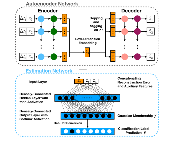
A schematic diagram of the neural network in this work is shown in Figure 1. It comprises of two sub-networks:
Autoencoder network:
Feature extraction is performed using the autoencoding RNN in Naul et al. (2018). The encoder and decoder each consist of two layers of Gated Recurrent Units (GRUs). A dropout layer is included between the two recurrent layers to avoid overfitting (Srivastava et al., 2014). Given a batch of $N$ normalized, phase-folded input light curve sequences $(\Delta\mathbf{t}_{i},\mathbf{x}_{i},\boldsymbol{\sigma}_{i})$, where $i$ denotes the $i$-th light curve, the encoder converts them into reduced-dimension embedding vectors, $\mathbf{z}_{\textrm{e},i}\in\mathbb{R}^{m}$. The dimension of the embedding vector, $m$, is a user-defined parameter called the embedding size. The embedding vectors are then used to reconstruct the input light curves $\hat{\mathbf{x}}_{i}$ by the decoder. Following Naul et al. (2018), the loss function to be minimized is the weighted mean square error,

$$L_{\textrm{AE}}=\frac{1}{n\;N}\sum_{i=1}^{N}\left(\mathbf{x}_{i}-\hat{\mathbf{x}}_{i}\right)^{2}\cdot\mathbf{w}_{i},$$ (1)

where $\mathbf{w}_{i}=1/\boldsymbol{\sigma}_{i}$ is the sample weight for each epoch, and the $\left(\cdot\right)^{2}$ is an element-wise operation. This loss function is advantageous over the conventional mean square error in that it explicitly includes measurement errors from irregularly sampled observations. Through minimization of the deviation between the input and reconstructed light curves, quantified by $L_{AE}$, the encoder is directed to produce embedding vectors that contain representative information of the original light curves.

Figure 2: Left: The normalized confusion matrix from the jointly trained autoencoder-estimation network. Right: Time evolution of the autoencoder loss $L_{\textrm{AE}}$ computed from the validation dataset during network training. The solid lines show the linearly smoothed trends. The lines with lighter colors shows the actual unsmoothed variations.

Estimation network:
Classification and novelty detection are simultaneously accomplished by the estimation network. The input feature vector to the estimation network is constructed by combining the autoencoder embedding $\mathbf{z}_{\textrm{e},i}$, two additional reconstruction error features $\mathbf{z}_{\textrm{r},i}$, and three auxiliary features $\mathbf{z}_{\textrm{a},i}$. Following Zong et al. (2018), the two reconstruction error features are the Euclidean distance and the cosine similarity,

$$\mathbf{z}_{\textrm{r},i}=\left[\frac{\left\|\mathbf{x}_{i}-\hat{\mathbf{x}}_{i}\right\|_{2}}{\left\|\mathbf{x}_{i}\right\|_{2}},\frac{\mathbf{x}_{i}\cdot\hat{\mathbf{x}}_{i}}{\left\|\mathbf{x}_{i}\right\|_{2}\left\|\hat{\mathbf{x}}_{i}\right\|_{2}}\right],$$ (2)

where $|\cdot|_{2}$ denotes the $L_{2}$ norm. The mean and standard deviation of each light curve sequence are combined with the variable’s period to form the auxiliary features, $\mathbf{z}_{\textrm{a},i}=\left(\langle\mathbf{x}_{i}\rangle,s_{i},\log_{10}(P_{i})\right)$. The input feature vector to the estimation network takes the form $\mathbf{z}_{i}~{}=~{}(\mathbf{z}_{\textrm{e},i},\mathbf{z}_{\textrm{r},i},\mathbf{z}_{\textrm{a},i})$, with dimension, $l=m+5$.

The estimation network connects the input feature vector to an output layer through a single densely connected hidden layer. The dimension of the output layer, $K$, is a pre-specified number of variable classes, which also corresponds to the number of Gaussian mixture components. A dropout layer is added after the hidden layer to minimize overfitting. The output layer ends with a softmax activation function, producing a $K$-dimensional, normalized vector, $\boldsymbol{\gamma}_{i}$, whose elements can be interpreted as the probabilities of belonging to each variable class/Gaussian component.

The classification functionality is trained by minimizing the categorical cross-entropy loss,

$$L_{\textrm{CE}}=-\frac{1}{N}\sum_{i=1}^{N}\mathbf{y}_{i}\cdot\log\left(\boldsymbol{\gamma}_{i}\right),$$ (3)

where $\mathbf{y}_{i}$ is the true label of the $i$-th light curve expressed as a $K$-dimensional one-hot vector, and the $\log$ is an element-wise natural logarithm on $\boldsymbol{\gamma_{i}}$. To generate the classification label predictions, the softmax outputs, $\boldsymbol{\gamma_{i}}$, are converted into one-hot vectors, $\hat{\mathbf{y}}_{i}$.

The feature vectors, $\mathbf{z}_{i}$, and the estimation network outputs, $\boldsymbol{\gamma}_{i}$, are used to compute the GMM parameters using Equation (5) of Zong et al. (2018). Following their notation, $\boldsymbol{\mu}_{k}$ is the mean location, $\boldsymbol{\Sigma}_{k}$ is the covariance matrix, and $\boldsymbol{\phi}_{k}$ is the me an membership probability of the $k$-th Gaussian component in the feature space. The sample energy of each light curve sequence can be computed by

$$E(\mathbf{z}_{i})=-\log\left(\sum_{k=1}^{K}{\phi}_{k}\;\xi_{k}(\mathbf{z}_{i})\right),$$ (4)

where $\xi_{k}$ is the normalized probability density in the $k$-th Gaussian component,

$$\xi_{k}(\mathbf{z}_{i})=\frac{\text{exp}(-\frac{1}{2}(\mathbf{z}_{i}-\boldsymbol{\mu}_{k})^{T}\mathbf{\boldsymbol{\Sigma}}_{k}^{-1}(\mathbf{z}_{i}-\boldsymbol{\mu}_{k}))}{\sqrt{(2\pi)^{l}\mathbf{\boldsymbol{|\Sigma}}_{k}|}},$$ (5)

$\log$ is the natural logarithm, and $|\cdot|$ denotes the matrix determinant. During network training, the GMM parameters are determined and the associated loss is minimized using

$$L_{\textrm{GMM}}=\frac{1}{N}\sum_{i=1}^{N}E(\mathbf{z}_{i}).$$ (6)

Optimizing the estimation network by minimizing $L_{\textrm{GMM}}$ is equivalent to fitting the GMM parameters by maximizing the log-likelihood. After training, the GMM parameters should adequately describe the distribution of variable types in the feature space. New forms of variability can then be detected as outliers far away from the Gaussian components.

The overall estimation network architecture follows Zong et al. (2018) closely, but there are two main differences. First, the network is tasked with the additional problem of classification. Second, with the addition of the classification loss, the GMM is not susceptible to the singularity problem. The covariance loss is therefore unnecessary and omitted.

Table 2: Classification accuracy and novelty detection performance for the fiducial network with an embedding size of 16. Numbers in parentheses correspond to results from networks trained using the additional photometric features.

		Joint Training	Sequential Training
Classification Accuracy	Estimation Network	98.8% (99.1%)	96.7% (96.6%)
	Random Forest	99.2% (99.4%)	99.2% (99.2%)
Novelty Detection Scores 95th Percentile Cutoff	Precision	0.885 (0.898)	0.875 (0.896)
	Recall	0.815 (0.957)	0.778 (0.933)
	$F_{1}$ score	0.848 (0.927)	0.824 (0.914)
Novelty Detection Scores 80th Percentile Cutoff	Precision	0.686 (0.700)	0.683 (0.696)
	Recall	0.941 (0.991)	0.935 (0.986)
	$F_{1}$ score	0.793 (0.821)	0.789 (0.816)

2.3 Training Strategies

The dual-network architecture was implemented using the Keras python package (Chollet et al., 2015) with a Tensorflow backend (Abadi et al., 2015). It was built on the GitHub implementation provided by Naul et al. (2018). The source code and a subset of the ASAS-SN data are available at https://github.com/bthtsang/Deep
ClassifierNoveltyDetection.

Weights and biases in both networks are initialized with the glorot_uniform initializer (Glorot & Bengio, 2010), and the loss function is minimized using the Adam optimizer (Kingma & Ba, 2014). We chose the same eight variable superclasses as used in Jayasinghe et al. (2018, Figure 29) so that direct comparisons can be made between classification performance. The variable subclasses that make up each superclass are summarized in Table 1.

To demonstrate the versatility of the dual-network, two training approaches have been carried out, namely, the joint and sequential training. In joint training, both the autoencoder and estimation network are optimized simultaneously by minimizing the total loss,

$$L_{\textrm{tot}}=L_{\textrm{AE}}+\left(\lambda L_{\textrm{GMM}}+L_{\textrm{CE}}\right),$$ (7)

where the pre-factor $\lambda$ controls the relative importance of the GMM component. Different values of $\lambda$ have been tested and a fiducial value of $10^{-3}$ works well for the current application. For sequential training, the autoencoder is first trained utilizing only the $L_{\textrm{AE}}$ loss, i.e. the exact training approach used in Naul et al. (2018). The estimation network is trained afterwards, minimizing the parenthesized loss terms of Equation (7). The motivation for including the sequentially trained models is twofold: it produces an independently trained autoencoder with which we can benchmark our classification accuracy, it also provides an opportunity to assess the possibility of attaching novelty detection functionality on pre-trained feature extraction approaches.

An 80/20 split is used to divide the light curve sequences into training and validation datasets. To preserve the percentages of sequences in each variable class, the partition is performed using the StratifiedKFold function of the python sklearn package. The validation dataset is withheld from the network during the entire training stage, and is used to determine the classification accuracy of the networks.

The following parameters are used in both training approaches. A total of 96 GRUs were used in both layers of the RNN autoencoder network. Training is done with a constant batch size of 2000 and learning rate of $2\times~{}10^{-4}$ for 2000 epochs. Dropout rates are fixed at 0.25 and 0.5 for the autoencoder and estimation network, respectively. We varied the embedding sizes between 8, 16, 32, and 64. The size of the hidden layer in the estimation network is fixed at the embedding size. As a benchmark, a separate grid of RF classifiers are trained using the encoder-generated features after network training. We adopted a grid of n_estimators $\in\{50,100,250\}$, criterion $\in\{\textrm{gini},\textrm{entropy}\}$, max_features $\in\{0.05,0.1,0.2,0.3\}$, and min_samples_leaf $\in\{1,2,3\}$ with the SKLEARN RandomForestClassifier implementation.

3 Results and discussions

3.1 Classification Accuracy

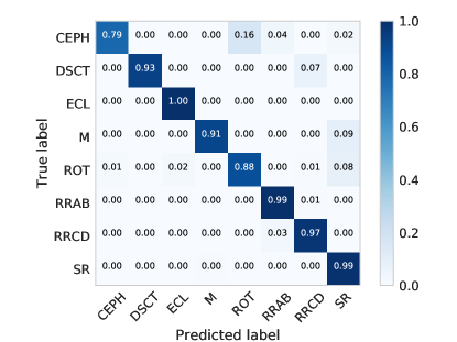
As embedding sizes of 8, 32 and 64 only offer marginally different performance in both classification and novelty detection, in this Letter, we will focus on the results from the fiducial models with an embedding size of 16. The normalized confusion matrix from the joint network training is shown on the left panel of Figure 2. The overall classification accuracy of the validation data is 98.8%. In particular, the classification performance on classes with copious amounts of light curves, namely ECL, RR Lyrae, and SR, is near-perfect. With sequential training, the classification accuracy falls slightly to 96.7%, primarily due to misclassifications in the less populated superclasses.

As a comparison, the best-performing RF classifier gives an accuracy of 99.2%, regardless of whether the network is trained jointly or sequentially. The higher accuracy of RF is expected given its complexity relative to the basic estimation network. In fact, the best-performing RF classifiers in the grid typically contain $\sim 10^{2}$ decision trees, each consists of $\sim 10^{2}$ nodes. A RF classifier therefore contains $\sim 10^{4}$ trainable parameters, whereas the densely-connected layers of the estimation network have $\sim 200-5000$, depending on the embedding size. The classification accuracy and novelty detection performance scores for both training approaches are summarized in Table 2.

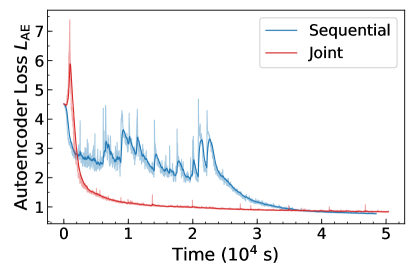
The right panel of Figure 2 shows the validation autoencoder loss over time during network training. The joint training approach offers more efficient training of the autoencoder, completing most of its learning early on after $10^{4}$ s, or just $\sim$200 epochs. Even though sequential training reaches slightly lower autoencoder loss by the end of the training, classification accuracy is lower nevertheless. It suggests that by simultaneously optimizing both networks, the autoencoder is able to better retain class-specific information for a more effective feature extraction. Across all embedding sizes (8, 16, 32, and 64), the joint training appeared to reduce stochastic fluctuations in the autoencoder loss, allowing superior, consistent training.

Figure 3: The energy histograms of the jointly trained network, without (left) and with (right) the inclusion of photometric features. An energy cap of 200 is imposed when creating the histograms for better visualization. The vertical dashed lines denote the 80th and 95th percentiles of the training set. The secondary peaks at $E\sim 50$ in the case with included photometric features are the result of missing magnitudes/colors, where a filling value of 99 is used.

3.2 Novelty Detection Performance

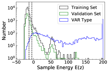
After the network training, the GMM parameters are computed and fixed using the entire training set. The VAR light curve sequences are mixed with the validation dataset to form the test dataset for novelty detection, which contains objects both from the superclasses and of the VAR type. Light curve sequences from the test dataset were then passed into the encoder to generate the embedding vectors. Together with the reconstruction error and auxiliary features, the sample energy of individual sequences can then be computed using Equation (4). Light curves with sample energies above a pre-selected percentile cutoff in the training set, e.g. at 80% or 95%, are flagged as novel samples.

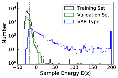
The left panel of Figure 3 shows the energy histogram of the light curve sequences in the training/validation dataset and of the VAR type. Although there is a slight amount of overlap below $E\sim 0$, the majority of the VAR objects have higher energy and are visually distinct. Using a 95th percentile cutoff, the precision, recall, and $F_{1}$ score are 0.885, 0.815, and 0.848, respectively. With sequential training, the performance scores are slight lower, at 0.875, 0.778, and 0.824 respectively. The reduction in recall implies that there are more VAR samples mixed into samples with low energies and went undetected, suggesting that the GMM components are not as well-fitted. The performance scores are also summarized in Table 2. Despite the lower accuracy and novelty detection scores, the performance of sequential training is satisfactory. It suggests that the estimation network can be readily integrated with existing classification pipelines with pre-computed features, e.g. from Fourier analysis, to deliver additional novelty detection functionality.

3.3 Inclusion of Photometric Information

The majority of mis-classification in the confusion matrix (Figure 2) appears among classes CEPH, M, and ROT, whose light curves are scarce and intrinsically similar to one another. Though all classes benefited from explicitly including the auxiliary features (mean magnitude, standard deviation, variable period), the three classes above require them for satisfactory classification accuracy. Since the estimation network is responsible for classification and novelty detection, it is expected that improved classification accuracy will allow GMM components to be better optimized for enhanced novelty detection.

Photometric quantities from external catalogs are appended as additional features in an attempt to refine classification accuracies and thus improve novelty detection. The photometric values were retrieved from the ASAS-SN Variable Stars Database and concatenated as part of the input features to the estimation network. As our current intention is to examine the feasibility of incorporating additional photometric features, only three catalog quantities are selected, namely, the Gaia DR2 $M_{\textrm{G}}$ magnitude, the $G_{\textrm{BP}}-G_{\textrm{RP}}$ color, and the Wesenheit Gaia $G_{\textrm{RP}}$ band magnitude $W_{\textrm{RP}}$. The three confused classes are distinctly separated in this color-magnitude space (Jayasinghe et al., 2018, Figure 22). All parameters of the network were held fixed while training with photometric features so a direct comparison can be made.

With the addition of the photometric information, the normalized accuracy in the CEPH, M, and ROT classes are boosted up to 84%, 93%, 93% respectively. The overall classification accuracy increases up to 99.1%. Most importantly, the novelty detection performance improved to reach an $F_{1}$ score of 0.93. This exercise demonstrates that embedded light curve features can be trivially integrated with photometric features for better multi-task performance.

4 Conclusions

We present a dual-network architecture that allows simultaneous training for feature extraction, classification, and novel sample detection of variable star light curves. We have combined the recurrent neural network autoencoder for time series data proposed by Naul et al. (2018) with the Gaussian mixture anomaly detection network proposed by Zong et al. (2018). Applied to light curves from the ASAS-SN variable star database, the networks achieve a classification accuracy of $\sim$99% and are able to detect previously unseen types of variability with a precision, recall, and $F_{1}$ score of $\geq 0.8-0.9$.

Joint training of the autoencoder and the classification/novelty detection network is found to be mutually beneficial, resulting in more efficient autoencoder training and better overall performance. When trained on pre-extracted features, the network nevertheless produces satisfactory results. It suggests that the Gaussian mixture-based network can be readily integrated with existing classification pipelines for the added functionality of novelty detection. Photometric features from external catalogs are found to be readily compatible with light curve features to deliver enhanced results.

This work demonstrates the flexibility and extensibility of unsupervised feature extraction of time series data for and beyond variable classification. The dual-network architecture also highlights the fidelity of deep neural networks in accomplishing multiple important tasks.

References

- Abadi et al. (2015) Abadi, M., Agarwal, A., Barham, P., et al. 2015, TensorFlow: Large-Scale Machine Learning on Heterogeneous Systems, , , software available from tensorflow.org. https://www.tensorflow.org/
- Aguirre et al. (2019) Aguirre, C., Pichara, K., & Becker, I. 2019, MNRAS, 482, 5078
- Aniyan & Thorat (2017) Aniyan, A. K., & Thorat, K. 2017, The Astrophysical Journal Supplement Series, 230, 20
- Bellm et al. (2019) Bellm, E. C., Kulkarni, S. R., Graham, M. J., et al. 2019, PASP, 131, 018002
- Bloom et al. (2012) Bloom, J. S., Richards, J. W., Nugent, P. E., et al. 2012, PASP, 124, 1175
- Cabrera-Vives et al. (2017) Cabrera-Vives, G., Reyes, I., Förster, F., Estévez, P. A., & Maureira, J.-C. 2017, ApJ, 836, 97
- Chollet et al. (2015) Chollet, F., et al. 2015, Keras, https://keras.io, ,
- Dieleman et al. (2015) Dieleman, S., Willett, K. W., & Dambre, J. 2015, MNRAS, 450, 1441
- Dubath et al. (2011) Dubath, P., Rimoldini, L., Süveges, M., et al. 2011, MNRAS, 414, 2602
- Glorot & Bengio (2010) Glorot, X., & Bengio, Y. 2010, in Proceedings of the Thirteenth International Conference on Artificial Intelligence and Statistics, AISTATS 2010, Chia Laguna Resort, Sardinia, Italy, May 13-15, 2010, 249–256. http://www.jmlr.org/proceedings/papers/v9/glorot10a.html
- Ivezić et al. (2008) Ivezić, Ž., Kahn, S. M., Tyson, J. A., et al. 2008, arXiv e-prints, arXiv:0805.2366
- Jayasinghe et al. (2018) Jayasinghe, T., Stanek, K. Z., Kochanek, C. S., et al. 2018, arXiv e-prints, arXiv:1809.07329
- Kim & Bailer-Jones (2016) Kim, D.-W., & Bailer-Jones, C. A. L. 2016, A&A, 587, A18
- Kim et al. (2014) Kim, D.-W., Protopapas, P., Bailer-Jones, C. A. L., et al. 2014, A&A, 566, A43
- Kingma & Ba (2014) Kingma, D. P., & Ba, J. 2014, arXiv e-prints, arXiv:1412.6980
- Kovács et al. (2002) Kovács, G., Zucker, S., & Mazeh, T. 2002, A&A, 391, 369
- Lomb (1976) Lomb, N. R. 1976, Ap&SS, 39, 447
- LSST Science Collaboration et al. (2009) LSST Science Collaboration, Abell, P. A., Allison, J., et al. 2009, arXiv e-prints, arXiv:0912.0201
- Masci et al. (2014) Masci, F. J., Hoffman, D. I., Grillmair, C. J., & Cutri, R. M. 2014, AJ, 148, 21
- Muthukrishna et al. (2019) Muthukrishna, D., Narayan, G., Mandel, K. S., Biswas, R., & Hložek, R. 2019, arXiv e-prints, arXiv:1904.00014
- Naul et al. (2018) Naul, B., Bloom, J. S., Pérez, F., & van der Walt, S. 2018, Nature Astronomy, 2, 151
- Nun et al. (2015) Nun, I., Protopapas, P., Sim, B., et al. 2015, arXiv e-prints, arXiv:1506.00010
- Reis et al. (2019) Reis, I., Baron, D., & Shahaf, S. 2019, AJ, 157, 16
- Richards et al. (2011) Richards, J. W., Starr, D. L., Butler, N. R., et al. 2011, ApJ, 733, 10
- Rimoldini et al. (2018) Rimoldini, L., Holl, B., Audard, M., et al. 2018, arXiv e-prints, arXiv:1811.03919
- Scargle (1982) Scargle, J. D. 1982, ApJ, 263, 835
- Schwarzenberg-Czerny (1996) Schwarzenberg-Czerny, A. 1996, ApJ, 460, L107
- Sedaghat & Mahabal (2018) Sedaghat, N., & Mahabal, A. 2018, MNRAS, 476, 5365
- Shallue & Vanderburg (2018) Shallue, C. J., & Vanderburg, A. 2018, AJ, 155, 94
- Shappee et al. (2014) Shappee, B. J., Prieto, J. L., Grupe, D., et al. 2014, ApJ, 788, 48
- Srivastava et al. (2014) Srivastava, N., Hinton, G., Krizhevsky, A., Sutskever, I., & Salakhutdinov, R. 2014, Journal of Machine Learning Research, 15, 1929. http://jmlr.org/papers/v15/srivastava14a.html
- Zong et al. (2018) Zong, B., Song, Q., Min, M. R., et al. 2018, in International Conference on Learning Representations. https://openreview.net/forum?id=BJJLHbb0-