On a Poincaré polynomial from Khovanov homology and Vassiliev invariants

Abstract.

We introduce a Poincaré polynomial with two-variable $t$ and $x$ for knots, derived from Khovanov homology, where the specialization $(t,x)$ $=$ $(1,-1)$ is a Vassiliev invariant of order $n$. Since for every $n$, there exist non-trivial knots with the same value of the Vassiliev invariant of order $n$ as that of the unknot, there has been no explicit formulation of a perturbative knot invariant which is a coefficient of $y^{n}$ by the replacement $q=e^{y}$ for the quantum parameter $q$ of a quantum knot invariant, and which distinguishes the above knots together with the unknot. The first formulation is our polynomial.

1. Introduction

Vassiliev [6] introduces his ordered invariants by using singularity theory. For the space $\mathcal{M}$ of all smooth maps from $S^{1}$ to $\mathbb{R}^{3}$, let $\Sigma$ be the set of maps which are not embeddings. Then, a filtration of subgroups $\{G_{n}\}_{n=1}^{\infty}$ of the reduced cohomology $\tilde{H}^{0}(\mathcal{M}\setminus\Gamma)$ is introduced. An element in $G_{n}\setminus G_{n-1}$ corresponds to an oriented knot $K$ gives us a knot invariant, which is so-called a Vassiliev invariant of order $n$. Birman and Lin [2] give a relation between the Jones polynomial and the Vassiliev invariant, i.e., for a one-variable polynomial $U_{x}(K)$ obtained from the Jones polynomial by replacing the variable with $e^{x}$, they show that for a power series $U_{x}(K)=\sum_{n=0}^{\infty}u_{n}(K)x^{n}$, each $u_{n}$ is a Vassiliev invariant of order $n$ (Fact 1).

In this paper, we consider an analogue of this Birman-Lin argument using Khovanov homology as follows. For an oriented link $L$, Khovanov [4] defines groups that are knot invariants and are so-called Khovanov homology $\mathcal{H}^{i,j}(L)$ such that

$$J(L)(q)=\sum_{i,j}(-1)^{i}q^{j}\,\operatorname{rank}\,\mathcal{H}^{i,j}(L),$$

where $J(L)(q)$ is a version of the Jones polynomial of $L$. It implies the Khovanov polynomial

$$\sum_{i,j}t^{i}q^{j}\,\operatorname{rank}\,\mathcal{H}^{i,j}(L)\quad(=Kh(L)(t,q)).$$

Using each coefficient $v_{n}(K)(t,x)$ of $y^{n}$ in $Kh(L)(t,q)|_{q=xe^{y}}$, we have:

Theorem 1.

Let $l$, $m$, and $n$ be integers where $2\leq l<m<n$. Let $v_{n}(K)(t,x)$ be a function as in Definition 4. Then, $v_{n}(K)(-1,1)$ is a Vassiliev invariant of order $n$ and there exists a set $\{K_{\mu}\}_{\mu\geq 2}$ consisting of oriented knots such that for a given tuple $(l,m,n)$, $v_{n}(K_{l})(-1,1)$ $=$ $v_{n}(K_{m})(-1,1)$ $=v_{n}(\operatorname{unknot})(-1,1)$ but $v_{n}(K_{l})(t,x)$ $\neq$ $v_{n}(K_{m})(t,x)$, $v_{n}(K_{l})(t,x)$ $\neq$ $v_{n}(\operatorname{unknot})(t,x)$, and $v_{n}(K_{m})(t,x)$ $\neq$ $v_{n}(\operatorname{unknot})(t,x)$.

Remark 1.

If $n=3$, $l=2$, there exists an oriented knot $K_{2}$ such that $v_{3}(K_{2})(-1,1)$ $=$ $v_{3}(\operatorname{unknot})(-1,1)$ wheres $v_{3}(K_{2})(t,x)$ $\neq$ $v_{3}(\operatorname{unknot})(t,x)$. The proof is placed on the end of Section 3.

Remark 2.

This $v_{n}(K)(t,x)$ equals $\sum_{i,j}\frac{j^{n}}{n!}t^{i}\operatorname{rank}\mathcal{H}^{i,j}(K)\,x^{j}$ (Lemma 1), which implies a triply graded homology $\mathcal{H}_{n}^{i,j}(K)$ by assigning $n$ to $\mathcal{H}^{i,j}(K)$ that belongs to the coefficient of $y^{n}$, i.e., a formula

$$Kh(L)(t,xe^{y})=\sum_{n=0}^{\infty}\sum_{i,j}\frac{j^{n}}{n!}t^{i}\,\operatorname{rank}\,\mathcal{H}^{i,j}_{n}(L)\,x^{j}y^{n},$$

satisfying $Kh(L)(-1,e^{y})$ $=$ $J_{L}(q)$ holds (cf. (1) of the proof of Lemma 1).

To the best our knowledge, there has been no explicit formulation of a perturbative knot invariant which is a coefficient of $y^{n}$ obtained from the replacement $q=e^{y}$ of the quantum parameter $q$ of a quantum knot invariant, and which distinguishes $K_{m}$ ($m\leq n-1$) of Theorem 1 (Figure 2) together with the unknot wheres the Vassiliev invariant cannot. The first formulation is our two-variable Poincaré polynomial $v_{n}(K_{n})(t,x)$ which is introduced in this paper, and which is the coefficient of $y^{n}$ and satisfies that the specialization $v_{n}(K_{n})(-1,1)$ is a Vassiliev invariant of order $n$. Further, it is interesting that though this polynomial invariant $v_{n}(K)(t,x)$ can detect the difference between $K_{m}$ ($m\leq n-1$) and the unknot, essentially, there exists a fixed number $j_{0}$ such that the coefficient $x^{j_{0}}y^{n}$ detect them (here, $j_{0}$ is actually the lowest degree of $x$ in $v_{n}(K)(t,x)$). It implies that an information of the $j$-grade of $v_{n}(K)(t,x)$ is useful (for the detail, see Section 3). In the literature, this usefulness of the grade implicitly appeared in a work of Kanenobu-Miyazawa [3], they showed that $V^{(n)}_{K}(1)$ is a Vassiliev invariant by using the $n$th derivative of the Jones polynomial $V_{K}(r)$.

The plan of the paper is as follows. We will prove Theorem 1 (Section 3) after we obtain definitions and notations (Section 2). In Section 4, we give a table of our function $v_{n,j}(K)(t,x)$ and its sum $v_{n}(K)(t,x)$.

2. Preliminaries

2.1. The Jones polynomial and the Vassiliev invariant

Definition 1 (normalized Jones polynomial).

Let $L$ be an oriented link. The Jones polynomial $V_{L}(r)$ is well-known, which is a polynomial in $\mathbb{Z}[r^{1/2},r^{-1/2}]$ that is determined by an isotopy class of $L$. The Jones polynomial $V_{L}(r)$ is defined by

$$V_{\text{unknot}}(r)=1,$$

$$r^{-1}V_{L_{+}}(r)-rV_{L_{-}}(r)=(r^{1/2}-r^{-1/2})V_{L_{0}}(r).$$

where links $L_{+}$, $L_{-}$, and $L_{0}$ are defined by Figure 1 and where Figure 1 corresponds to local figures are included on a neighborhood and the exteriors of the three neighborhoods are the same.

     

$$L_{+}\qquad\qquad L_{-}\qquad\qquad L_{0}$$

Figure 1. Local figures $L_{+}$, $L_{-}$, and $L_{0}$ of an oriented link.

Definition 2 (unnormalized Jones polynomial).

Letting $q=-r^{1/2}$, we define an unnormalized Jones polynomial $J_{L}(q)$ by

$$J_{L}(q)|_{q=-r^{1/2}}=(-r^{1/2}-r^{-1/2})V_{L}(r).$$

By definition, $J_{L}(q)$ is a polynomial in $\mathbb{Z}[q,q^{-1}]$ that is determined by an isotopy class of $L$. Let $L_{+}$, $L_{-}$, and $L_{0}$ be as in Definition 1. Then, the polynomial $J_{L}(q)$ satisfies

$$J_{\text{unknot}}(q)=q+q^{-1},$$

$$q^{-2}J_{L_{+}}(q)-q^{2}J_{L_{-}}(q)=(q^{-1}-q)J_{L_{0}}(q).$$

Fact 1 (Birman-Lin, Theorem of [2]).

Let $K$ be a knot and let $V_{K}(r)$ be its Jones polynomial as in Definition 1. Let $U_{x}(K)$ be obtained from $V_{K}(r)$ by replacing the variable $r$ by $e^{x}$. Express $U_{x}(K)$ as a power series in $x$:

$$U_{x}(K)=\sum_{i=0}^{\infty}u_{i}(K)x^{i}.$$

Then, $u_{0}(K)=1$ and each $u_{i}(K)$, $i\geq 1$ is a Vassiliev invariant of order $i$.

2.2. A polynomial invariant from Khovanov polynomial

Definition 3.

Let $L$ be a link and $\mathcal{H}^{i,j}(L)$ the Khovanov homology group of $L$. The Khovanov polynomial is defined by

$$Kh(L)(t,q)=\sum_{i,j}t^{i}q^{j}\,\operatorname{rank}\,\mathcal{H}^{i,j}(L).$$

Definition 4 (two-variable polynomials).

Let $Kh(K)(t,q)|_{q=xe^{y}}$ be a polynomial obtained from the Khovanov polynomial $Kh(K)(t,q)$ by replacing the variable $q$ with $xe^{y}$. Then, let $v_{n}(K)(t,x)$ the coefficient of $y^{n}$ and let $v_{n,j}(K)(t,x)$ be (the coefficient of $x^{j}y^{n}$) $\cdot$ $x^{j}$.

By definition, $v_{n}(K)(t,x)$ $=\sum_{j}v_{n,j}(K)(t,x)$. It is clear that every $v_{n,j}(K)(t,x)$ is a link invariant, which implies that $v_{n}(K)(t,x)$ is also a link invariant. Definition 3 and Definition 4 imply Lemma 1.

Lemma 1.

$$v_{n,j}(K)(t,x)=\frac{j^{n}}{n!}\sum_{i}t^{i}\operatorname{rank}\mathcal{H}^{i,j}(K)\,x^{j}.$$

As a corollary,

$$v_{n}(K)(t,x)=\sum_{i,j}\frac{j^{n}}{n!}t^{i}\operatorname{rank}\mathcal{H}^{i,j}(K)\,x^{j}.$$

Proof.

$$Kh(L)(t,xe^{y}) =\sum_{j}(e^{y})^{j}x^{j}\sum_{i}t^{i}\,\operatorname{rank}\,\mathcal{H}^{i,j}(L)$$

$$=\sum_{j}\sum_{n=0}^{\infty}\frac{(jy)^{n}}{n!}x^{j}\sum_{i}t^{i}\,\operatorname{rank}\,\mathcal{H}^{i,j}(L)$$

$$=\sum_{j}\sum_{n=0}^{\infty}\frac{j^{n}}{n!}\sum_{i}t^{i}\,\operatorname{rank}\,\mathcal{H}^{i,j}(L)\,x^{j}y^{n}.$$

Then, the coefficient of $x^{j}y^{n}$ is $\frac{j^{n}}{n!}\sum_{i}t^{i}\,\operatorname{rank}\,\mathcal{H}^{i,j}(L)$. This fact together with Definition 4 of $v_{n,j}(K)(t,x)$, we have

$$v_{n,j}(K)(t,x)=\frac{j^{n}}{n!}\sum_{i}t^{i}\,\operatorname{rank}\,\mathcal{H}^{i,j}(L)\,x^{j}.$$

As a corollary,

$$v_{n}(K)(t,x)=\sum_{j}v_{n,j}(K)(t,x)=\sum_{i,j}\frac{j^{n}}{n!}t^{i}\operatorname{rank}\mathcal{H}^{i,j}(K)\,x^{j}.$$

∎

Lemma 2.

The integer $v_{n}(K)(-1,1)$ is a Vassiliev invariant of order $n$.

As a corollary, every Vassiliev invariant of order $n$ has a presentation

$$v_{n}(K)(-1,1)=\sum_{j}v_{n,j}(K)(-1,1).$$

Proof.

Using the above proof of Lemma 1, setting $x=1$ and $t=-1$, we have

(1) $$J(L)(q)|_{q={e^{y}}}=Kh(L)(-1,e^{y}) =\sum_{j}\sum_{n=0}^{\infty}\frac{j^{n}}{n!}\sum_{i}(-1)^{i}\,\operatorname{rank}\,\mathcal{H}^{i,j}(L)\,y^{n}.$$

The coefficient of $y^{n}$ is $\sum_{j}\frac{j^{n}}{n!}\sum_{i}(-1)^{i}\,\operatorname{rank}\,\mathcal{H}^{i,j}(L)$, which is $v_{n}(K)(-1,1)$. Then, by the same argument as [2, Proof of Theorem 4.1] of Birman-Lin, it is elementary to prove that the coefficient of $y^{n}$ of $J(L)(q)|_{q={e^{y}}}$ is a Vassiliev invariant of order $n$. This fact and Lemma 1 imply the formula of the claim. ∎

3. A proof of Theorem 1.

Since Lemma 2 holds, we should the latter part of the claim. For this proof, we use notations and definitions of Khovanov homology as in [7]. Although it is sufficient to use $\mathbb{Z}/2\mathbb{Z}$-homology, here we use $\mathbb{Z}$-homology to avoid adding notations of symbols. We recall that a chain group $\mathcal{C}^{i,j}(D)$ of an oriented link diagram $D$. In particular, for each enhanced state of $\mathcal{C}^{i,j}(D)$, $i(S)=\frac{w(D)-\sigma(s)}{2}$ and $j(S)=w(D)$ $+$ $i(S)$ $+$ $\tau(S)$ (for definition of a state $s$, an enhanced state $S$, the writhe number $w(D)$, a sum $\sigma(s)$ of signs , and a sum $\tau(S)$ of signs, see [7]).

Let $m$ be a positive integer $(m\geq 2)$ and $K_{n}$ a knot with a fixed $m$ that is defined by Figure 2. It is well-known that for every Vassiliev invariant $v_{n}$ of order $n$, $v_{n}(\operatorname{unknot})=0$ and $v_{n}(K_{m})=0$ ($m\leq n-1$) [5], which implies that $v_{n}(K_{l})(-1,1)$ $=$ $v_{n}(K_{m})(-1,1)$ $=$ $v_{n}(\operatorname{unknot})(-1,1)$ ($\because$ Lemma 2).

Let $D_{m}$ be a knot diagram defined by Figure 2, $s_{n}$ a state defined by Figure 3 (a), and $S_{n}$ a state defined by Figure 3 (b).

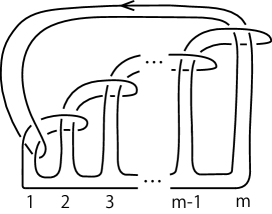
Figure 2. A diagram of a knot $K_{m}$.

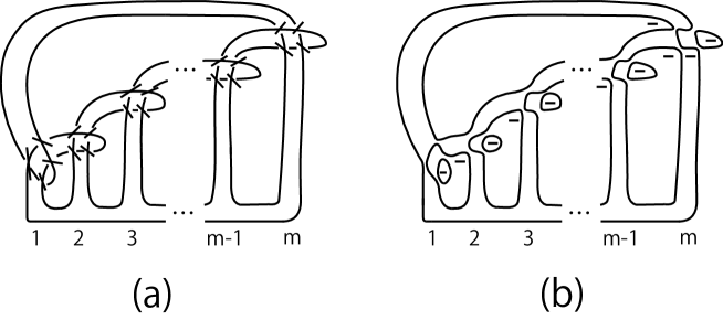
Figure 3. (a) the state $s$ of $K_{m}$ (each short edge indicates the direction of smoothing of a crossing) and (b) the enhanced state $S$ of $K_{m}$ (each sign indicates a sign of a circle).

Note that by the definition of this $\mathbb{Z}$-homology, $S_{m}$ obtains the minimum number of degree $i$ is $-2m$ and the minimum number of degree $j$ is $-4m-1$ as follows:

$$w(D_{m})=0,$$

$$i(S_{m})=\frac{0-4m}{2}=-2m,~{}{\textrm{and}}~{}$$

$$j(S_{m})=0+(-2m)+(-1-2m)=-4m-1.$$

Note also that by the definition of the differential $d:\mathcal{C}^{i,j}(D)$ $\to$ $\mathcal{C}^{i+1,j}(D)$, $d^{-2m}(S_{m})$ $=$ $0$ and ${\operatorname{Im}}d^{-2m-1}=0$. Then, for each $m$ ($\geq 2$),

(2) $$\mathcal{H}^{-2m,-4m-1}(K_{m})=\mathbb{Z}.$$

By Lemma 1,

$$v_{n,j}(K)(t,x)=\sum_{i}t^{i}\operatorname{rank}\mathcal{H}^{i,j}(K)\,x^{j}.$$

We focus on the minimum number of $i$ that is $-2m$, and the minimum number of $j$ that is $-4m-1$. Setting $i=-2m$ and $j=-4m-1$, the coefficient of $t^{-2m}x^{-4m-1}$ in $v_{n,-4m-1}(K)(t,x)$ is

$$\frac{(-4m-1)^{n}}{n!}\operatorname{rank}\mathcal{H}^{-2m,-4m-1}(K).$$

Then, (2) implies

$$\frac{(-4m-1)^{n}}{n!}\operatorname{rank}\mathcal{H}^{-2m,-4m-1}(K_{m})=\frac{(-4m-1)^{n}}{n!}.$$

Thus, for every pair $l,m$ ($2\leq l<m$), $v_{n,-4l-1}(K_{l})(t,x)$ $=$ $\frac{(-4l-1)^{n}}{n!}$ $\neq$ $\frac{(-4m-1)^{n}}{n!}$ $=$ $v_{n,-4m-1}(K_{m})(t,x)$. Here, recall that for the unknot, it is well-known that $Kh(\operatorname{unknot})(t,q)$ $=$ $q^{-1}$ $+$ $q$, which implies that there is no non-trivial coefficient of $t^{k}$ $(k\neq 0)$, i.e., any non-trivial part corresponds to the coefficient $q+q^{-1}$, which belongs to the coefficient of $t^{0}$. It implies $v_{n,-4l-1}(K_{l})(t,x)$ $\neq$ $v_{n,-4l-1}(\operatorname{unknot})(t,x)$ and $v_{n,-4m-1}(K_{m})(t,x)$ $\neq$ $v_{n,-4m-1}(\operatorname{unknot})(t,x)$.

Note that for every knot $K_{l}$ ($2\leq l$), the minimum number of $j$ is $-4l-1$, by always focusing on the lowest degree of $x$ in $v_{n}(K)(t,x)$ ($=$ $\sum_{j}v_{n,j}(K)(t,x)$), the above argument works since the coefficient of the lowest degree of $x$ exactly equals $v_{n,-4l-1}(K)(t,x)$. Therefore, by focusing the case $j=-4l-1$ or the case $j=-4m-1$, for every pair $l,m$ ($2\leq l<m$), $v_{n}(K_{l})(t,x)$ $\neq$ $v_{n}(K_{m})(t,x)$, $v_{n}(K_{l})(t,x)$ $\neq$ $v_{n}(\operatorname{unknot})(t,x)$ and $v_{n}(K_{m})(t,x)$ $\neq$ $v_{n}(\operatorname{unknot})(t,x)$ since for each case, two lowest degrees are different. It completes the proof of Theorem 1. $\hfill\Box$

Proof of Remark 1. Note that the coefficient of $t^{-2\cdot 2}x^{-4\cdot 2-1}$ in $v_{3,-9}(K_{2})(t,x)$ is $\frac{(-4\cdot 2-1)^{3}}{3!}$. Thus, $v_{3,-9}(K_{2})(t,x)$ $\neq$ $v_{3,-9}(\operatorname{unknot})(t,x)$. By focusing on the lowest degree of $x$ in $v_{3}(K)(t,x)$ ($=$ $\sum_{j}v_{3,j}(K)(t,x)$), we have the statement of Remark 1. $\hfill\Box$

4. Table

We give some examples of the Khovanov polynomial and the two-variables polynomials for a few prime knots. We use the data of the Khovanov polynomial in the Mathematica package KnotTheory [1] and attach a Mathematica file to arXiv page.

$$\begin{array}[]{|c|c|}\hline\cr\text{Knot}&3_{1}\\ \hline\cr\text{Kh}&q^{9}t^{3}+q^{5}t^{2}+q^{3}+q\\ \hline\cr v_{0}&t^{3}x^{9}+t^{2}x^{5}+x^{3}+x\\ \hline\cr v_{1}&9t^{3}x^{9}+5t^{2}x^{5}+3x^{3}+x\\ \hline\cr v_{2}&\frac{81t^{3}x^{9}}{2}+\frac{25t^{2}x^{5}}{2}+\frac{9x^{3}}{2}+\frac{x}{2}\\ \hline\cr v_{3}&\frac{243t^{3}x^{9}}{2}+\frac{125t^{2}x^{5}}{6}+\frac{9x^{3}}{2}+\frac{x}{6}\\ \hline\cr v_{4}&\frac{2187t^{3}x^{9}}{8}+\frac{625t^{2}x^{5}}{24}+\frac{27x^{3}}{8}+\frac{x}{24}\\ \hline\cr v_{5}&\frac{19683t^{3}x^{9}}{40}+\frac{625t^{2}x^{5}}{24}+\frac{81x^{3}}{40}+\frac{x}{120}\\ \hline\cr\end{array}$$

$$\begin{array}[]{|c|c|}\hline\cr\text{Knot}&4_{1}\\ \hline\cr\text{Kh}&q^{5}t^{2}+\frac{1}{q^{5}t^{2}}+qt+\frac{1}{qt}+q+\frac{1}{q}\\ \hline\cr v_{0}&t^{2}x^{5}+\frac{1}{t^{2}x^{5}}+tx+\frac{1}{tx}+x+\frac{1}{x}\\ \hline\cr v_{1}&5t^{2}x^{5}-\frac{5}{t^{2}x^{5}}+tx-\frac{1}{tx}+x-\frac{1}{x}\\ \hline\cr v_{2}&\frac{25t^{2}x^{5}}{2}+\frac{25}{2t^{2}x^{5}}+\frac{tx}{2}+\frac{1}{2tx}+\frac{x}{2}+\frac{1}{2x}\\ \hline\cr v_{3}&\frac{125t^{2}x^{5}}{6}-\frac{125}{6t^{2}x^{5}}+\frac{tx}{6}-\frac{1}{6tx}+\frac{x}{6}-\frac{1}{6x}\\ \hline\cr v_{4}&\frac{625t^{2}x^{5}}{24}+\frac{625}{24t^{2}x^{5}}+\frac{tx}{24}+\frac{1}{24tx}+\frac{x}{24}+\frac{1}{24x}\\ \hline\cr v_{5}&\frac{625t^{2}x^{5}}{24}-\frac{625}{24t^{2}x^{5}}+\frac{tx}{120}-\frac{1}{120tx}+\frac{x}{120}-\frac{1}{120x}\\ \hline\cr\end{array}$$

$$\begin{array}[]{|c|c|}\hline\cr\text{Knot}&5_{1}\\ \hline\cr\text{Kh}&q^{15}t^{5}+q^{11}t^{4}+q^{11}t^{3}+q^{7}t^{2}+q^{5}+q^{3}\\ \hline\cr v_{0}&t^{5}x^{15}+t^{4}x^{11}+t^{3}x^{11}+t^{2}x^{7}+x^{5}+x^{3}\\ \hline\cr v_{1}&15t^{5}x^{15}+11t^{4}x^{11}+11t^{3}x^{11}+7t^{2}x^{7}+5x^{5}+3x^{3}\\ \hline\cr v_{2}&\frac{225t^{5}x^{15}}{2}+\frac{121t^{4}x^{11}}{2}+\frac{121t^{3}x^{11}}{2}+\frac{49t^{2}x^{7}}{2}+\frac{25x^{5}}{2}+\frac{9x^{3}}{2}\\ \hline\cr v_{3}&\frac{1125t^{5}x^{15}}{2}+\frac{1331t^{4}x^{11}}{6}+\frac{1331t^{3}x^{11}}{6}+\frac{343t^{2}x^{7}}{6}+\frac{125x^{5}}{6}+\frac{9x^{3}}{2}\\ \hline\cr v_{4}&\frac{16875t^{5}x^{15}}{8}+\frac{14641t^{4}x^{11}}{24}+\frac{14641t^{3}x^{11}}{24}+\frac{2401t^{2}x^{7}}{24}+\frac{625x^{5}}{24}+\frac{27x^{3}}{8}\\ \hline\cr v_{5}&\frac{50625t^{5}x^{15}}{8}+\frac{161051t^{4}x^{11}}{120}+\frac{161051t^{3}x^{11}}{120}+\frac{16807t^{2}x^{7}}{120}+\frac{625x^{5}}{24}+\frac{81x^{3}}{40}\\ \hline\cr\end{array}$$

$$\begin{array}[]{|c|c|}\hline\cr\text{Knot}&5_{2}\\ \hline\cr\text{Kh}&q^{13}t^{5}+q^{9}t^{4}+q^{9}t^{3}+q^{7}t^{2}+q^{5}t^{2}+q^{3}t+q^{3}+q\\ \hline\cr v_{0}&t^{5}x^{13}+t^{4}x^{9}+t^{3}x^{9}+t^{2}x^{7}+t^{2}x^{5}+tx^{3}+x^{3}+x\\ \hline\cr v_{1}&13t^{5}x^{13}+9t^{4}x^{9}+9t^{3}x^{9}+7t^{2}x^{7}+5t^{2}x^{5}+3tx^{3}+3x^{3}+x\\ \hline\cr v_{2}&\frac{169t^{5}x^{13}}{2}+\frac{81t^{4}x^{9}}{2}+\frac{81t^{3}x^{9}}{2}+\frac{49t^{2}x^{7}}{2}+\frac{25t^{2}x^{5}}{2}+\frac{9tx^{3}}{2}+\frac{9x^{3}}{2}+\frac{x}{2}\\ \hline\cr v_{3}&\frac{2197t^{5}x^{13}}{6}+\frac{243t^{4}x^{9}}{2}+\frac{243t^{3}x^{9}}{2}+\frac{343t^{2}x^{7}}{6}+\frac{125t^{2}x^{5}}{6}+\frac{9tx^{3}}{2}+\frac{9x^{3}}{2}+\frac{x}{6}\\ \hline\cr v_{4}&\frac{28561t^{5}x^{13}}{24}+\frac{2187t^{4}x^{9}}{8}+\frac{2187t^{3}x^{9}}{8}+\frac{2401t^{2}x^{7}}{24}+\frac{625t^{2}x^{5}}{24}+\frac{27tx^{3}}{8}+\frac{27x^{3}}{8}+\frac{x}{24}\\ \hline\cr v_{5}&\frac{371293t^{5}x^{13}}{120}+\frac{19683t^{4}x^{9}}{40}+\frac{19683t^{3}x^{9}}{40}+\frac{16807t^{2}x^{7}}{120}+\frac{625t^{2}x^{5}}{24}+\frac{81tx^{3}}{40}+\frac{81x^{3}}{40}+\frac{x}{120}\\ \hline\cr\end{array}$$

$$\begin{array}[]{|c|c|}\hline\cr\text{Knot}&6_{1}\\ \hline\cr\text{Kh}&q^{9}t^{4}+q^{5}t^{3}+q^{5}t^{2}+\frac{1}{q^{5}t^{2}}+q^{3}t+qt+\frac{1}{qt}+q+\frac{2}{q}\\ \hline\cr v_{0}&t^{4}x^{9}+t^{3}x^{5}+t^{2}x^{5}+\frac{1}{t^{2}x^{5}}+tx^{3}+tx+\frac{1}{tx}+x+\frac{2}{x}\\ \hline\cr v_{1}&9t^{4}x^{9}+5t^{3}x^{5}+5t^{2}x^{5}-\frac{5}{t^{2}x^{5}}+3tx^{3}+tx-\frac{1}{tx}+x-\frac{2}{x}\\ \hline\cr v_{2}&\frac{81t^{4}x^{9}}{2}+\frac{25t^{3}x^{5}}{2}+\frac{25t^{2}x^{5}}{2}+\frac{25}{2t^{2}x^{5}}+\frac{9tx^{3}}{2}+\frac{tx}{2}+\frac{1}{2tx}+\frac{x}{2}+\frac{1}{x}\\ \hline\cr v_{3}&\frac{243t^{4}x^{9}}{2}+\frac{125t^{3}x^{5}}{6}+\frac{125t^{2}x^{5}}{6}-\frac{125}{6t^{2}x^{5}}+\frac{9tx^{3}}{2}+\frac{tx}{6}-\frac{1}{6tx}+\frac{x}{6}-\frac{1}{3x}\\ \hline\cr v_{4}&\frac{2187t^{4}x^{9}}{8}+\frac{625t^{3}x^{5}}{24}+\frac{625t^{2}x^{5}}{24}+\frac{625}{24t^{2}x^{5}}+\frac{27tx^{3}}{8}+\frac{tx}{24}+\frac{1}{24tx}+\frac{x}{24}+\frac{1}{12x}\\ \hline\cr v_{5}&\frac{19683t^{4}x^{9}}{40}+\frac{625t^{3}x^{5}}{24}+\frac{625t^{2}x^{5}}{24}-\frac{625}{24t^{2}x^{5}}+\frac{81tx^{3}}{40}+\frac{tx}{120}-\frac{1}{120tx}+\frac{x}{120}-\frac{1}{60x}\\ \hline\cr\end{array}$$

$$\begin{array}[]{|c|c|}\hline\cr\text{Knot}&6_{2}\\ \hline\cr\text{Kh}&q^{11}t^{4}+q^{9}t^{3}+q^{7}t^{3}+q^{7}t^{2}+q^{5}t^{2}+q^{5}t+\frac{1}{q^{3}t^{2}}+q^{3}t+q^{3}+\frac{q}{t}+2q\\ \hline\cr v_{0}&t^{4}x^{11}+t^{3}x^{9}+t^{3}x^{7}+t^{2}x^{7}+t^{2}x^{5}+\frac{1}{t^{2}x^{3}}+tx^{5}+tx^{3}+\frac{x}{t}+x^{3}+2x\\ \hline\cr v_{1}&11t^{4}x^{11}+9t^{3}x^{9}+7t^{3}x^{7}+7t^{2}x^{7}+5t^{2}x^{5}-\frac{3}{t^{2}x^{3}}+5tx^{5}+3tx^{3}+\frac{x}{t}+3x^{3}+2x\\ \hline\cr v_{2}&\frac{121t^{4}x^{11}}{2}+\frac{81t^{3}x^{9}}{2}+\frac{49t^{3}x^{7}}{2}+\frac{49t^{2}x^{7}}{2}+\frac{25t^{2}x^{5}}{2}+\frac{9}{2t^{2}x^{3}}+\frac{25tx^{5}}{2}+\frac{9tx^{3}}{2}+\frac{x}{2t}+\frac{9x^{3}}{2}+x\\ \hline\cr v_{3}&\frac{1331t^{4}x^{11}}{6}+\frac{243t^{3}x^{9}}{2}+\frac{343t^{3}x^{7}}{6}+\frac{343t^{2}x^{7}}{6}+\frac{125t^{2}x^{5}}{6}-\frac{9}{2t^{2}x^{3}}+\frac{125tx^{5}}{6}+\frac{9tx^{3}}{2}+\frac{x}{6t}+\frac{9x^{3}}{2}+\frac{x}{3}\\ \hline\cr v_{4}&\frac{14641t^{4}x^{11}}{24}+\frac{2187t^{3}x^{9}}{8}+\frac{2401t^{3}x^{7}}{24}+\frac{2401t^{2}x^{7}}{24}+\frac{625t^{2}x^{5}}{24}+\frac{27}{8t^{2}x^{3}}+\frac{625tx^{5}}{24}+\frac{27tx^{3}}{8}+\frac{x}{24t}+\frac{27x^{3}}{8}+\frac{x}{12}\\ \hline\cr v_{5}&\frac{161051t^{4}x^{11}}{120}+\frac{19683t^{3}x^{9}}{40}+\frac{16807t^{3}x^{7}}{120}+\frac{16807t^{2}x^{7}}{120}+\frac{625t^{2}x^{5}}{24}-\frac{81}{40t^{2}x^{3}}+\frac{625tx^{5}}{24}+\frac{81tx^{3}}{40}+\frac{x}{120t}+\frac{81x^{3}}{40}+\frac{x}{60}\\ \hline\cr\end{array}$$

$$\begin{array}[]{|c|c|}\hline\cr\text{Knot}&6_{3}\\ \hline\cr\text{Kh}&q^{7}t^{3}+\frac{1}{q^{7}t^{3}}+q^{5}t^{2}+\frac{1}{q^{5}t^{2}}+q^{3}t^{2}+\frac{1}{q^{3}t^{2}}+q^{3}t+\frac{1}{q^{3}t}+qt+\frac{1}{qt}+2q+\frac{2}{q}\\ \hline\cr v_{0}&t^{3}x^{7}+\frac{1}{t^{3}x^{7}}+t^{2}x^{5}+\frac{1}{t^{2}x^{5}}+t^{2}x^{3}+\frac{1}{t^{2}x^{3}}+tx^{3}+\frac{1}{tx^{3}}+tx+\frac{1}{tx}+2x+\frac{2}{x}\\ \hline\cr v_{1}&7t^{3}x^{7}-\frac{7}{t^{3}x^{7}}+5t^{2}x^{5}-\frac{5}{t^{2}x^{5}}+3t^{2}x^{3}-\frac{3}{t^{2}x^{3}}+3tx^{3}-\frac{3}{tx^{3}}+tx-\frac{1}{tx}+2x-\frac{2}{x}\\ \hline\cr v_{2}&\frac{49t^{3}x^{7}}{2}+\frac{49}{2t^{3}x^{7}}+\frac{25t^{2}x^{5}}{2}+\frac{25}{2t^{2}x^{5}}+\frac{9t^{2}x^{3}}{2}+\frac{9}{2t^{2}x^{3}}+\frac{9tx^{3}}{2}+\frac{9}{2tx^{3}}+\frac{tx}{2}+\frac{1}{2tx}+x+\frac{1}{x}\\ \hline\cr v_{3}&\frac{343t^{3}x^{7}}{6}-\frac{343}{6t^{3}x^{7}}+\frac{125t^{2}x^{5}}{6}-\frac{125}{6t^{2}x^{5}}+\frac{9t^{2}x^{3}}{2}-\frac{9}{2t^{2}x^{3}}+\frac{9tx^{3}}{2}-\frac{9}{2tx^{3}}+\frac{tx}{6}-\frac{1}{6tx}+\frac{x}{3}-\frac{1}{3x}\\ \hline\cr v_{4}&\frac{2401t^{3}x^{7}}{24}+\frac{2401}{24t^{3}x^{7}}+\frac{625t^{2}x^{5}}{24}+\frac{625}{24t^{2}x^{5}}+\frac{27t^{2}x^{3}}{8}+\frac{27}{8t^{2}x^{3}}+\frac{27tx^{3}}{8}+\frac{27}{8tx^{3}}+\frac{tx}{24}+\frac{1}{24tx}+\frac{x}{12}+\frac{1}{12x}\\ \hline\cr v_{5}&\frac{16807t^{3}x^{7}}{120}-\frac{16807}{120t^{3}x^{7}}+\frac{625t^{2}x^{5}}{24}-\frac{625}{24t^{2}x^{5}}+\frac{81t^{2}x^{3}}{40}-\frac{81}{40t^{2}x^{3}}+\frac{81tx^{3}}{40}-\frac{81}{40tx^{3}}+\frac{tx}{120}-\frac{1}{120tx}+\frac{x}{60}-\frac{1}{60x}\\ \hline\cr\end{array}$$

References

- [1] D. Bar-Natan, S. Morrison, and et al. The Knot Atlas, http://katlas.org.
- [2] J. S. Birman and X.-S. Lin, Knot polynomials and Vassiliev’s invariants, Invent. Math. 111 (1993), 225–270.
- [3] T. Kanenobu and Y. Miyazawa, HOMFLY polynomials as Vassiliev invariants, Knot theory (Warsaw, 1995), 165–185, Banach Center Publ., 42, Polish Acad. Sci. Inst. Math., Warsaw, 1998.
- [4] M. Khovanov, A categorification of the Jones polynomial, Duke Math. J. 101 (2000), 359–426.
- [5] Y. Ohyama, Vassiliev invariants and similarity of knots, Proc. Amer. Math. Soc. 123 (1995), 287–291.
- [6] V. A. Vassiliev, Cohomology of knot spaces, Theory of singularities and its applications, 23–69, Adv. Soviet Math., 1, Amer. Math. Soc., Providence, RI, 1990.
- [7] O. Viro, Khovanov homology, its definitions and ramifications, Fund. Math. 184 (2004), 317–342.
- [8] M. Aganagic and S. Shakirov. Knot homology and refined Chern-Simons index. Commun. Math. Phys. 333(1) (2015): 187-228.