Adaptive Exponential Integrators for MCTDHF

Abstract

We compare exponential-type integrators for the numerical time-propagation of the equations of motion arising in the multi-configuration time-dependent Hartree-Fock method for the approximation of the high-dimensional multi-particle Schrödinger equation. We find that among the most widely used integrators like Runge-Kutta, exponential splitting, exponential Runge-Kutta, exponential multistep and Lawson methods, exponential Lawson multistep methods with one predictor/corrector step provide optimal stability and accuracy at the least computational cost, taking into account that the evaluation of the nonlocal potential terms is by far the computationally most expensive part of such a calculation. Moreover, the predictor step provides an estimator for the time-stepping error at no additional cost, which enables adaptive time-stepping to reliably control the accuracy of a computation.

1 Introduction

We compare time integration methods for nonlinear Schrödinger-type equations

$${\mathrm{i}}\,\partial_{t}u(t)=A\,u(t)+B(u(t))=H(u(t)),~{}\,t>t_{0},\quad u(t_{0})=u_{0},$$ (1)

on the Hilbert space $\mathcal{B}{{=L^{2}}}$. Here, $A\colon\mathcal{D}\subseteq\mathcal{B}\to\mathcal{B}$ is a self-adjoint differential operator and $B$ a generally unbounded nonlinear operator. Our focus is on the equations of motion associated with the multi-configuration time-dependent Hartree-Fock (MCTDHF) approximation to the multi-particle electronic Schrödinger equation, where the key issue is the high computational effort for the evaluation of the nonlocal (integral) operator $B$. Thus, in the choice of the most appropriate integrator, we emphasize a minimal number of evaluations of $B$ for a given order and disregard the effort for the propagation of $A$, which can commonly be realized at essentially the cost of two (cheap) transforms between real and frequency space via fast transforms like [I]FFT. The approaches that we pursue and advocate in this paper are thus based on splitting of the vector fields in (1). It turns out that exponential integrators hocost10 based on the variation of constants serve our purpose best, as they provide a desirable balance between computational effort and stability.

2 The MCTDHF method

We focus on the comparison of numerical methods for the equations of motion associated with MCTDHF for the approximate solution of the time-dependent multi-particle Schrödinger equation

$${\mathrm{i}}\,\frac{\partial\psi}{\partial t}=H\psi,$$

where the complex-valued wave function $\psi=\psi(x_{1},\dots,x_{f},t)$ depends on time $t$ and, in the case considered here, the positions $x_{1},\dots,x_{f}\in\mathbf{R}^{3}$ of electrons in an atom or molecule. The time-dependent Hamiltonian reads

$$H = H(t):=\sum_{k=1}^{f}\Big{(}\,\frac{1}{2}\,\Delta^{(k)}+U(x_{k})+\sum_{\ell<k}V(x_{k}-x_{\ell})\Big{)}+V_{\mathrm{ext}}(x_{1},\dots,x_{f},t)$$

$$=: T+W(t,x_{1},\dots,x_{f}),$$

$$T = \sum_{k=1}^{f}\frac{1}{2}\,\Delta^{(k)},\quad U(x)=-\frac{Z}{|x|},~{}Z\in\mathbf{N},\quad V(x-y)=\frac{1}{|x-y|}\,.$$

Here $V_{\mathrm{ext}}(x_{1},\dots,x_{f},t)$ is a smooth time-dependent function, and $\Delta^{(k)}$ is the Laplace operator with respect to $x_{k}$ only.

In MCTDHF as put forward in zanghellinietal03c , the multi-electron wave function $\psi$ is approximated by a function $u$ living in a manifold $\mathcal{M}$ characterized by the ansatz

$$u=\sum_{(j_{1},\dots,j_{f})}a_{j_{1},\dots,j_{f}}(t)\,\phi_{j_{1}}(x_{1},t)\cdots\phi_{j_{f}}(x_{f},t)=:\sum_{J}a_{J}(t)\,\Phi_{J}(x,t).$$ (2)

For the electronic Schrödinger equation, the Pauli principle implies that only solutions $u$ are considered which are antisymmetric under exchange of any pair of arguments $x_{j},x_{k}$,

Now, the Dirac-Frenkel variational principle frenkel34 in conjunction with orthogonality conditions is used to derive differential equations for the coefficients $a_{J}$ and the so-called single-particle functions $\phi_{j}$ in (2), where we will henceforth tacitly identify $u$ with the vector $(a,\phi)$ of coefficients and orbitals,

$${\mathrm{i}}\,\frac{da_{J}}{dt}=\sum_{K}\big{\langle}\Phi_{J}\left|W\right|\Phi_{K}\big{\rangle}\,a_{K}\quad\forall J,$$ (3)

$${\mathrm{i}}\,\frac{\partial\phi_{j}}{\partial t}=T\,\phi_{j}+(I-P)\sum_{k=1}^{N}\sum_{\ell=1}^{N}\rho^{-1}_{j,\ell}\,\overline{W}_{\ell,k}\,\phi_{k},\quad j=1,\dots,N,$$ (4)

where

$$\overline{W}_{j,\ell}=\big{\langle}\psi_{j}|W|\,\psi_{\ell}\big{\rangle},\quad\mbox{with}\quad\psi_{j}=\big{\langle}\phi_{j}\,|\,u\big{\rangle},~{}~{}\rho_{j,\ell}=\big{\langle}\psi_{j}\,|\,\psi_{\ell}\big{\rangle},$$

and where $P$ is the orthogonal projector onto the space spanned by the functions $\phi_{j}$. We will henceforth denote

$$A=\frac{{\mathrm{i}}}{2}\Big{(}0,\Delta^{(1)},\dots,0,\Delta^{(f)}\Big{)}^{T},\quad B=B(a,\phi),$$ (5)

where $B$ is the vector of the components associated with the potential which constitute the computationally most expensive part.

2.1 Splitting methods

Popular integrators for quantum dynamics are exponential time-splitting methods which are based on multiplicative combinations of the partial flows $\mathcal{E}_{A}(t,u)\colon$ $u\mapsto u(t)={\mathrm{e}}^{tA}\,u$ and $\mathcal{E}_{B}(t,u)\colon u\mapsto u(t)$ with $u^{\prime}(t)=B(u(t)),\;u(0)=u$. For a single step $(t_{n},u_{n})\mapsto(t_{n+1},u_{n+1})$ with time-step $h$, this reads

$$u_{n+1}:=\mathcal{S}(h,u_{n})=\mathcal{E}_{B}(b_{s}h,\cdot)\circ\mathcal{E}_{A}(a_{s}h,\cdot)\circ\ldots\circ\mathcal{E}_{B}(b_{1}h,\cdot)\circ\mathcal{E}_{A}(a_{1}h,u_{n}),$$

where the coefficients $a_{j},b_{j},\,j=1\ldots s$ are determined according to the requirement that a prescribed order of consistency is obtained haireretal02 . For a convergence analysis of splitting methods in the context of MCTDHF, see for instance knth10a .

2.2 Exponential integrators

An approach which also exploits the separated vector fields is given by the class of exponential integrators, which are comprehensively discussed in hocost10 . Here the variation of constant formula is used to express the solution of (1) for a time-step $t_{n}\to t_{n+1}=t_{n}+h$ via the integral equation

$$u(t_{n}+h)={\mathrm{e}}^{hA}\,u_{n}+\int_{0}^{h}{\mathrm{e}}^{(h-\tau)A}B(u(t_{n}+\tau))\,\mathrm{d}\tau.$$ (6)

Different numerical integrators are distinguished depending on how the integral in (6) is approximated.

Exponential Runge-Kutta methods

When the integral in (6) is approximated by a quadrature formula of Runge-Kutta type, relying on evaluations of the nonlinear operator $B$ at interior points $t_{n}+h\tau_{j},\ \tau_{j}\in[0,1],\ j=1,\dots,k$, an exponential Runge-Kutta method is obtained. This corresponds to replacing $B(\cdot)$ in the integrand by a polynomial interpolant at the points

$$\big{(}t_{n}+h\tau_{1},B(u(t_{n}+h\tau_{1})\big{)},\dots,\big{(}(t_{n}+h\tau_{k},B(u(t_{n}+h\tau_{k})\big{)}.$$

The method is realized by stepping from $t_{n}+h\tau_{j}\to t_{n}+h\tau_{j+1}$ in the same way as for a Runge-Kutta method, with appropriate weights of the stages. For implicit methods, nonlinear systems of equations have to be solved, which is generally considered as prohibitive. Note that after interpolation, the resulting integral can be evaluated analytically by using the $\varphi$-functions or alternatively, by numerical quadrature hocost10 . Such a procedure has first been proposed in friedli78 , for a stiff error analysis, see hocost10 and references therein. For our comparisons, we use the fourth order Krogstad method mentioned there.

Exponential multistep methods

The integral in (6) can be approximated in terms of an interpolation polynomial at previous approximations

$$\big{(}-(k-1)\,h,B(u_{n-k+1})\big{)},\dots,\big{(}(-h,B(u_{n-1})),(0,B(u_{n})\big{)}\,.$$ (7)

This yields an (explicit) exponential Adams-Bashforth multistep method first mentioned in certaine60 , and introduced more systematically in noersett69 , see also for instance calvopal11 ; hocost10 . If the interpolation also comprises the forward point $(h,B(u_{n+1}))$, an (implicit) exponential Adams-Moulton method is obtained. These two approaches can be combined in a predictor/corrector method in the same way as for linear multistep methods. Exponential multistep methods have first been considered and analyzed in calvopal11 under the assumption of smooth $B$, and a starting strategy is also given there.

Lawson methods

In Lawson methods, equation (1) is transformed prior to the numerical integration by the substitution $u(t)\to{\mathrm{e}}^{-tA}\,u(t)$. To the resulting equation

$$u^{\prime}(t)={\mathrm{e}}^{-tA}B\,({\mathrm{e}}^{tA}\,u(t))=:F(u(t)),$$ (8)

any appropriate time-stepping scheme can be applied. The main advantage lies in the fact that the dynamics associated with the non-smooth operator $A$ is separated by the transformation which can be realized cheaply in frequency space, while the problem subjected to the time-stepping scheme is smoother, thus allowing for larger time-steps. This transformation was first introduced in lawson67 for ordinary differential equations.

In a one-step version, an explicit Runge–Kutta method is employed to solve (8), which is equivalent to interpolation at interior nodes of the whole integrand in (6) by a polynomial in the same fashion as in (7). Reference hocost17 gives a convergence proof of Lawson Runge-Kutta methods in the stiff case, however under the assumption that the operator $B$ is smooth, which is not the case in the MCTDHF equations we are considering. A convergence proof for Adams-Lawson multistep methods for the MCTDHF equations under minimal regularity requirements is given in the forthcoming work koch19 . The proof addresses the transformed equation (8) and combines stability and consistency to conclude convergence. To this end, a boot-strapping argument is employed, first showing convergence in the Sobolev space $H^{1}$. Stability in $L^{2}$ only holds if the numerical solution is in $H^{1}$, which follows from the first argument, whence convergence in $L^{2}$ is inferred. Lipschitz conditions for the right-hand side entering the stability arguments can be shown by appropriate Sobolev-type inequalities in both $H^{1}$ and $L^{2}$. To prove consistency, the norms of derivatives of $F$ in (8) are estimated, which amounts to bounds on commutators of the operators $A$ and $B$. This implies assumptions on the regularity of the exact solution $u$.

We will demonstrate that the best approach for our goal is to use exponential Lawson multistep methods in a predictor/corrector implementation, which is shown to increase the accuracy and also provides a local error estimator for adaptive time-stepping at no additional cost. The efficiency of the time discretization can be improved if high-order time propagators are employed. In the multistep approach, this does not imply additional computational cost if no memory limitations have to be taken into account.

Comparisons

To assess the performance of the exponential integration methods described above, we will also show results for the classical explicit Runge-Kutta method of fourth order (RK4) and the second-order Strang splitting.

3 Numerical results

To illustrate the performance of our numerical methods, we consider MCTDHF with the choice $N=4$ for a one-dimensional model of a helium atom investigated in zanghellinietal03c , where

$$H(t)=H_{0}+(x_{1}+x_{2})\,\mathcal{E}(t),$$

$$H_{0}=-\frac{1}{2}(\partial_{x_{1}}^{2}+\partial_{x_{2}}^{2})-\frac{2}{\sqrt{x_{1}^{2}+b^{2}}}-\frac{2}{\sqrt{x_{2}^{2}+b^{2}}}+\frac{1}{\sqrt{(x_{1}-x_{2})^{2}+b^{2}}},$$

with a smoothed Coulomb potential with shielding parameter $b=0.7408$, which is irradiated by a short, intense, linearly polarized laser pulse

$$\mathcal{E}(t)=\mathcal{E}_{0}\,g(t)\sin(\omega t).$$

The peak amplitude is set to $\mathcal{E}_{0}=0.1894$, the frequency is $\omega=0.1837$, and we define the envelope $g(t)=1.2\exp\big{(}-5\cdot 10^{-4}\left(t-6\pi/\omega\right)^{2}\big{)}$. The parameters are taken from zanghellinietal03c , and the envelope is a smooth approximation of the trapezoidal envelope chosen there. In zanghellinietal03c , this model serves to illustrate the effect of correlation on the probability density along the diagonal $x=y$, which implies that the single-configuration Hartree–Fock approximation is insufficient. We first investigate stable long-time propagation in Fig. 1. We monitor norm conservation of the wave function in the propagation of the ground state for the Hamiltonian $H_{0}=H(0)$ for different equidistant stepsizes to resolve precisely the onset of instability. For RK4, the number of steps is specified in the plot; for all other methods, the number of steps is in $\{1000,2000,\dots,12000\}$. If norm conservation is violated beyond the effect of numerical accuracy, the method cannot be recommended for physical applications. Indeed, we observe the following: Explicit Runge-Kutta methods only behave in a stable way when the numerical accuracy is already very high, close to round-off error. Exponential multistep methods behave stably only for short times, even when a corrector step is performed. Exponential Runge-Kutta and Runge-Kutta-Lawson methods behave stably, likewise as splitting methods. Adams-Lawson multistep methods behave very stably, a corrector step adds to the accuracy, as well as providing an error estimate as the basis for adaptive time-stepping. The unstable exponential multistep methods are no longer considered. While showing the same stability behavior, the Yoshida splitting is demonstrated to be less efficient than the Suzuki splitting, and the low order (but popular) Strang splitting is not competitive. Higher-order multistep methods provide higher accuracy at the same computational effort irrespective of the order, and are thus also considered for this comparison.

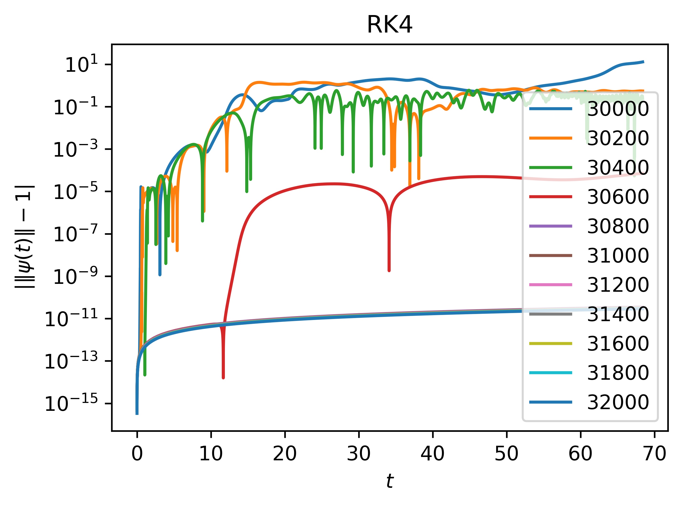
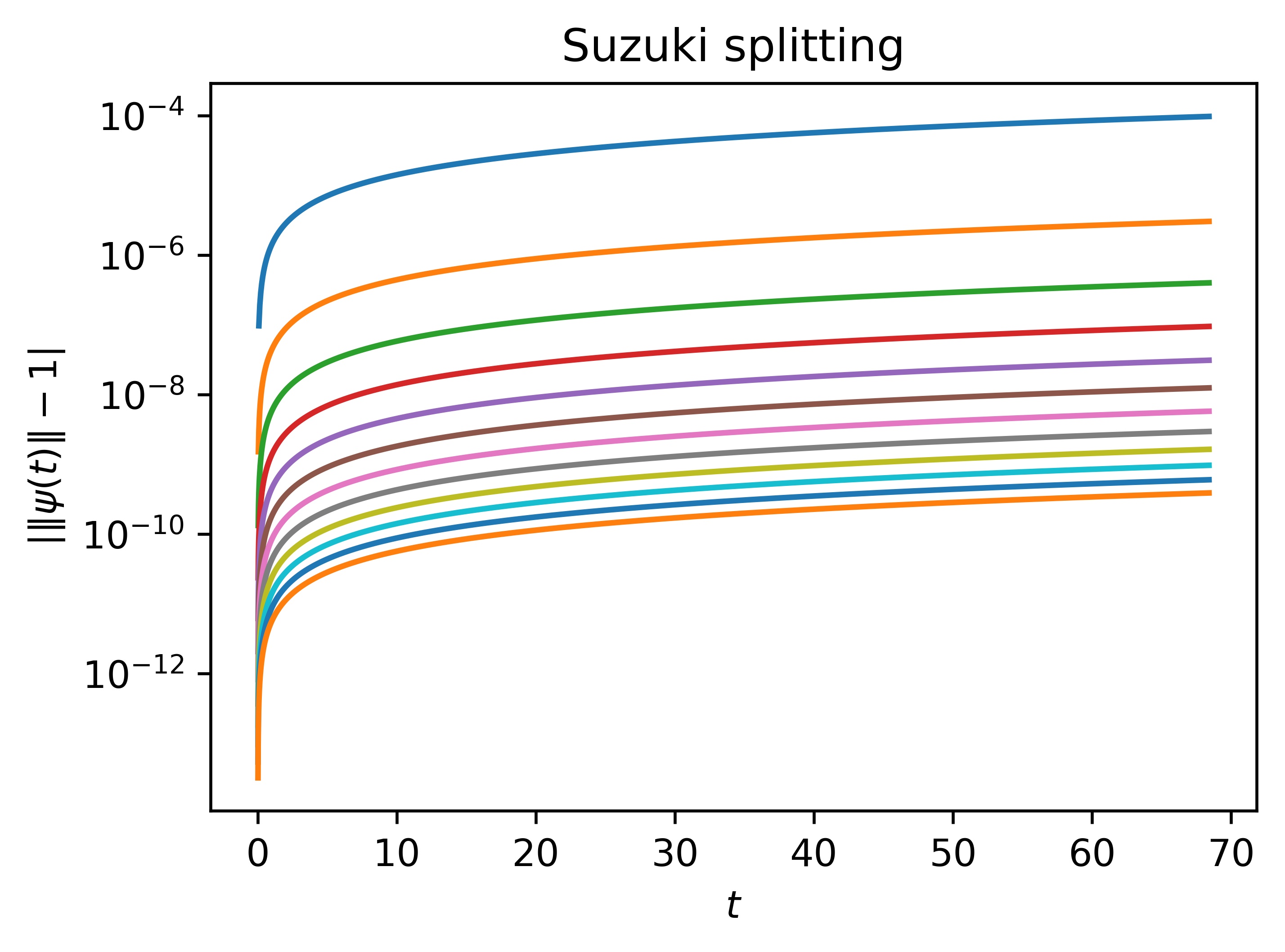
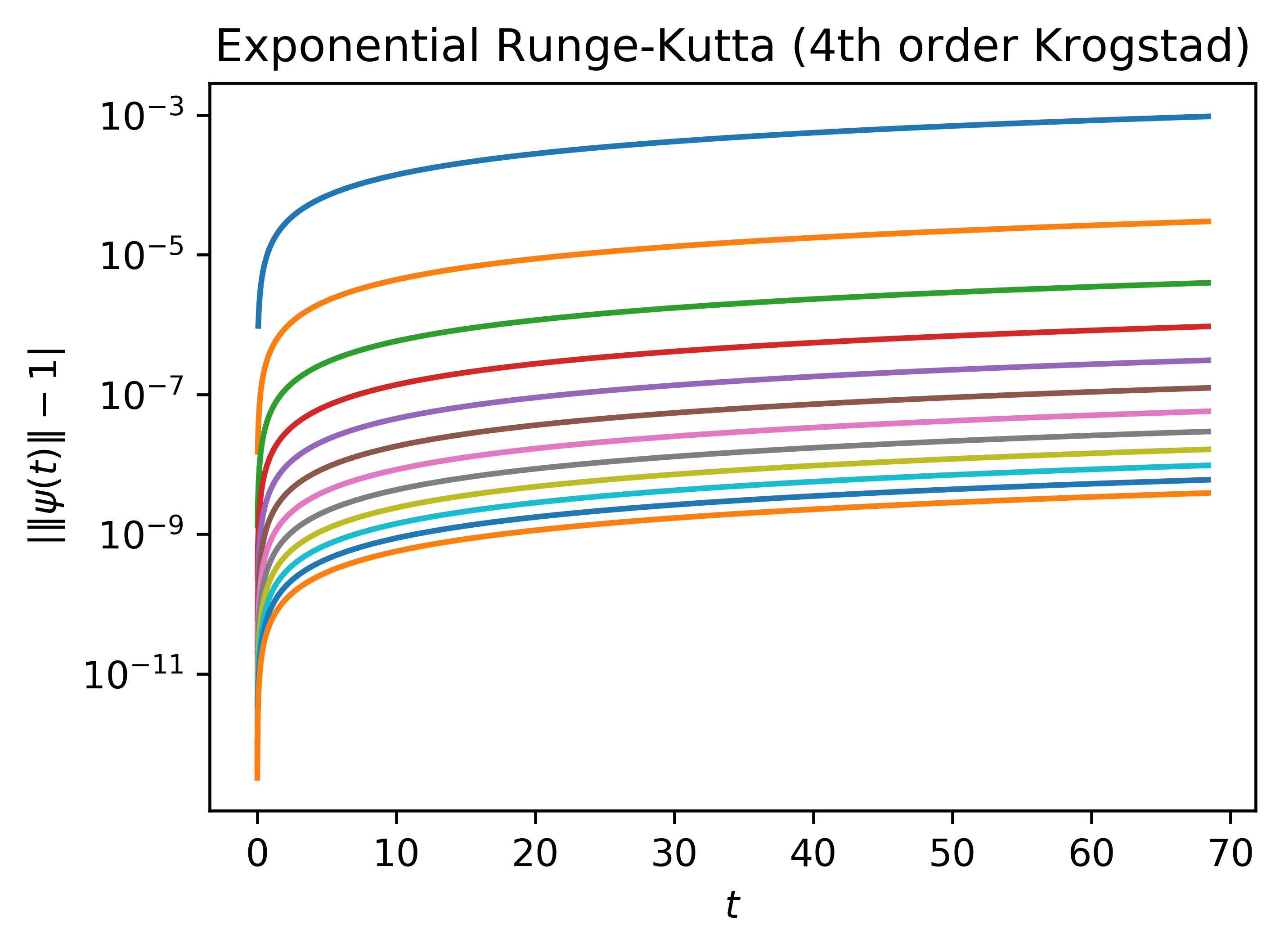
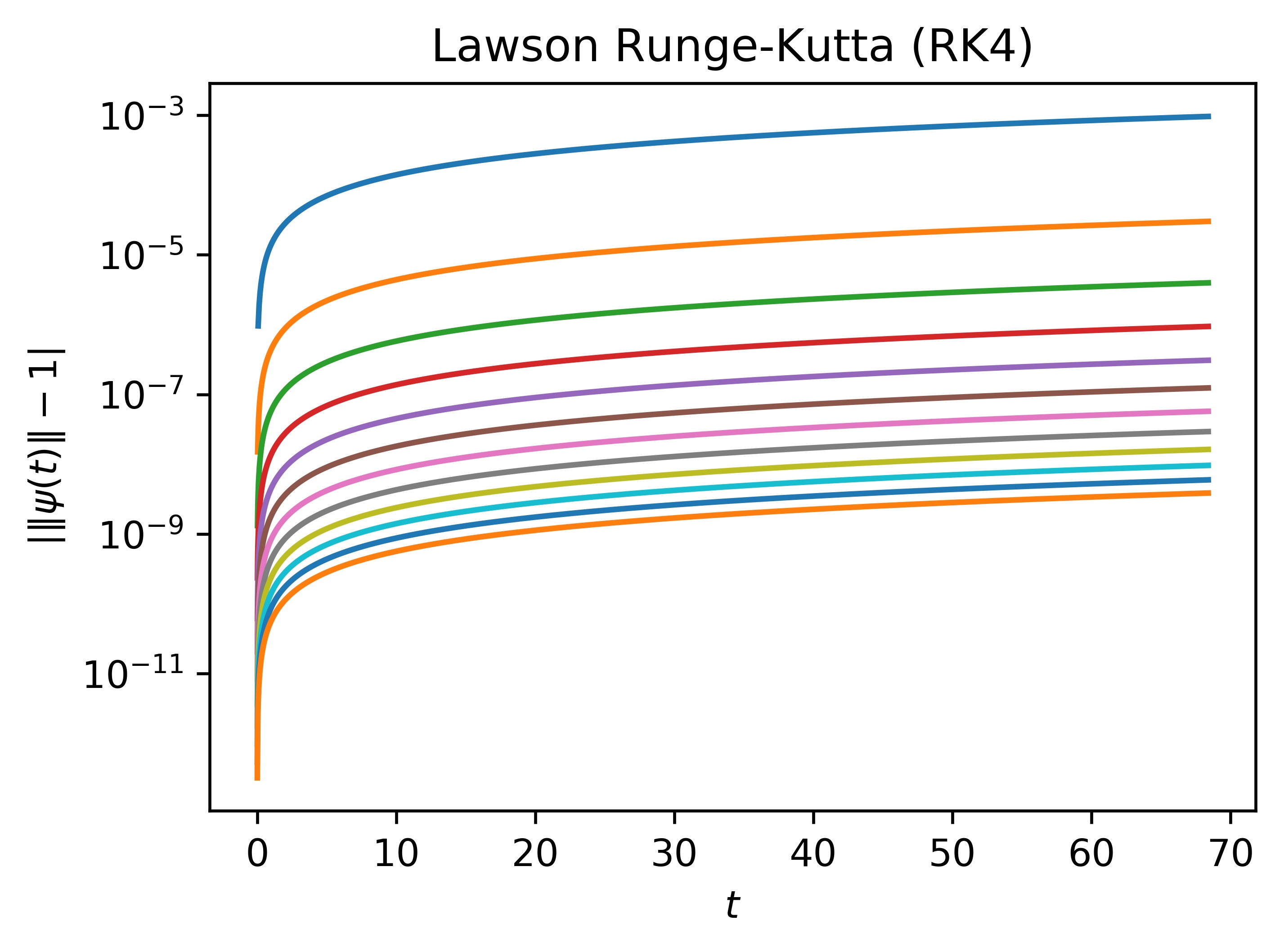
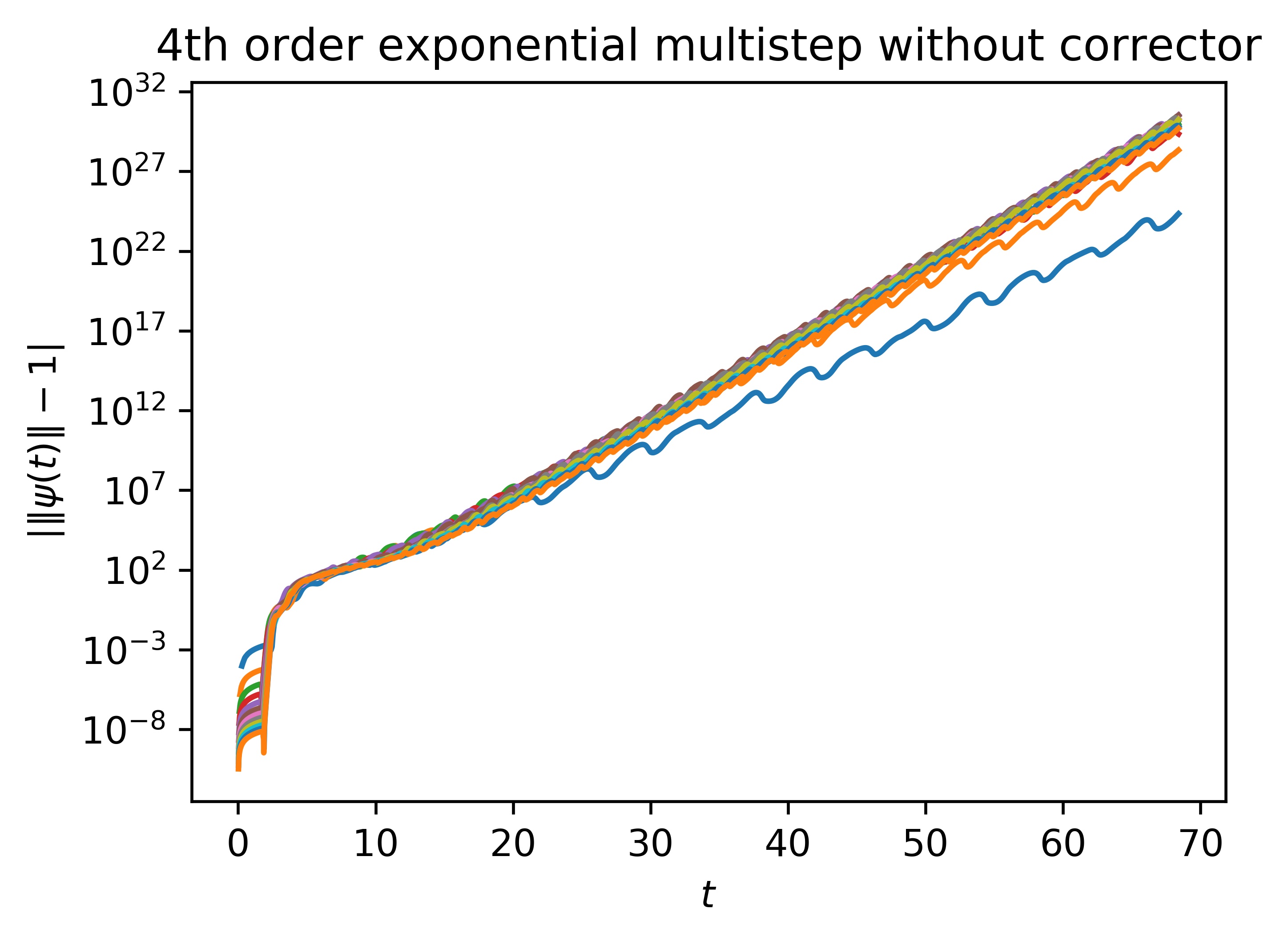
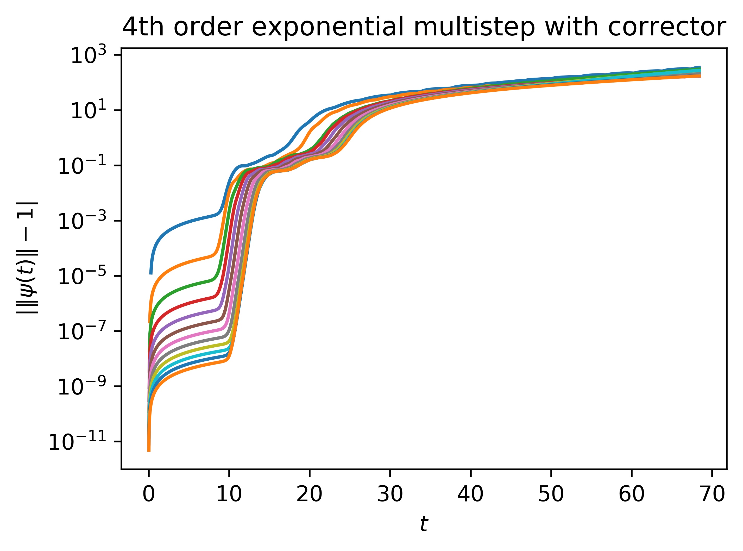
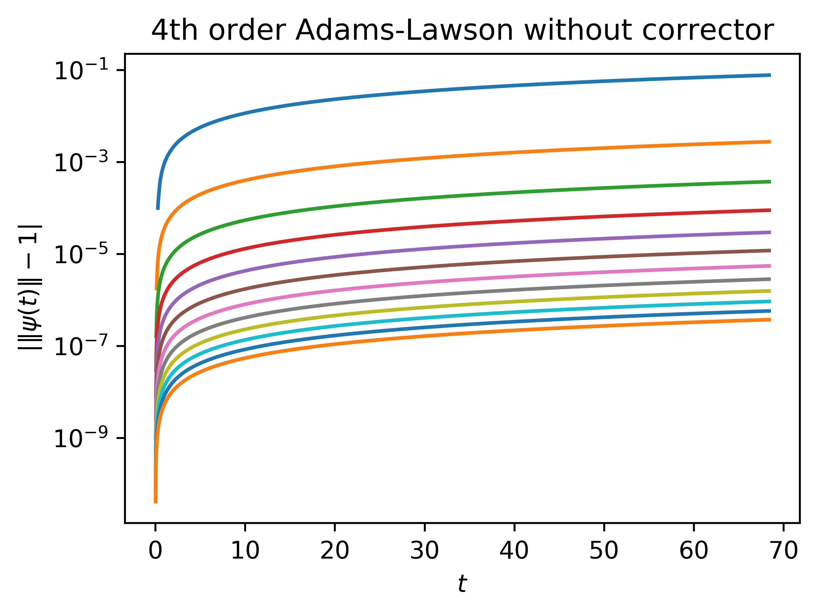
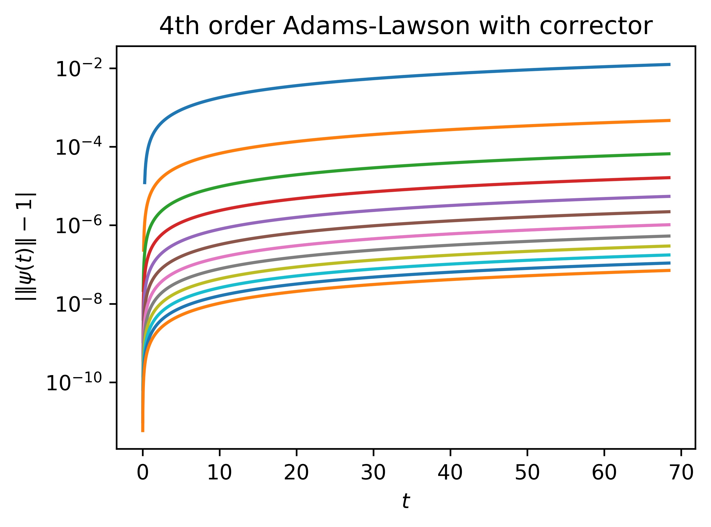
Figure 1: Comparison of stable long-time integration.

Next, we compare the efficiency of the different integrators. The unstable exponential multistep methods are no longer considered. While showing the same stability behavior, the Yoshida splitting is demonstrated to be less efficient than the Suzuki splitting, and the low order (but popular) Strang splitting is not competitive. High-order multistep methods provide higher accuracy at the same computational effort and are thus also considered for this comparison. To this end, we plot in Fig. 2 the accuracy as compared to a very precise reference solution at $t=80$ as a function of the number of evaluations of the computationally expensive potential part $B$ (dots on solid lines). Furthermore, we give the CPU time required in a sequential implementation on one thread of the Vienna Scientific Cluster (VSC) 3 comprising one Intel Xeon E5-2650v2 processor with 8 kernels of 2.6 gHz (crosses ‘$\times$’). We note that, as expected, the runtime is proportional to the number of potential evaluations. We observe that high-order Lawson multistep methods perform best, where particularly the high order which can be achieved in the multistep versions without additional evaluations is advantageous. Splitting methods, particularly the low order Strang splitting, are not very efficient due to the high effort for the propagation of the potential.

We stress that this shows only the picture on uniform grids. The multistep versions show their biggest advantage in adaptive time-stepping due to the cheap means of error estimation in the predictor/corrector implementation. To demonstrate that this works reliably for Adams-Lawson methods, we show in Fig. 3 the laser field $\mathcal{E}(t)$ and total energy functional (top) illustrating the local solution smoothness, and the stepsizes (bottom) automatically generated for the Adams-Lawson method of order 6. We see that the adaptively chosen stepsizes reflect the smoothness of the time evolution and the Lawson method enables larger stepsizes. The Adams-Lawson solution has been confirmed to be converged to within the prescribed tolerance $10^{-5}$. On the other hand, the corresponding exponential multistep method (without the Lawson transformation) shows a noticeable deviation in the solution.

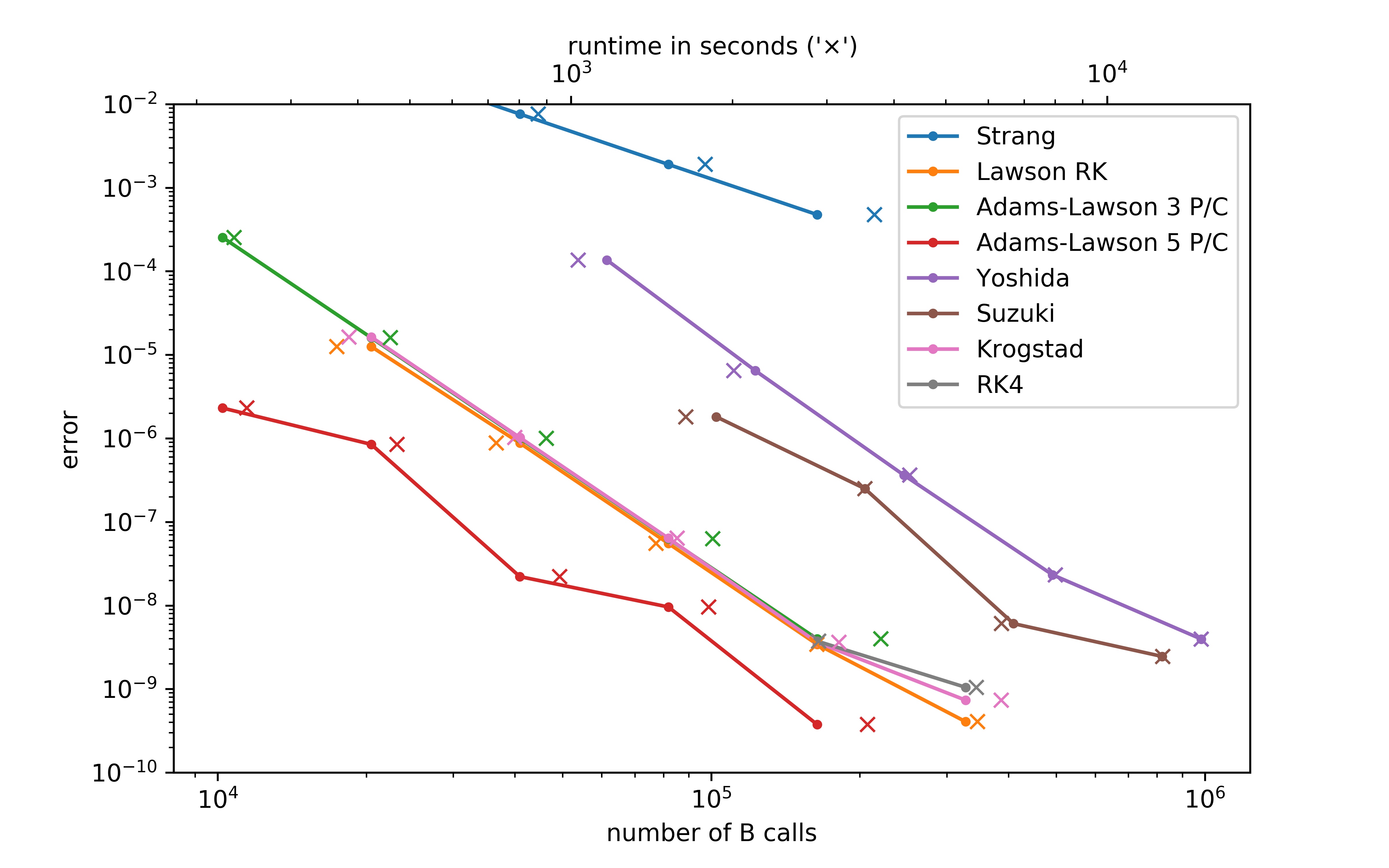
Figure 2: Work/precision comparison for the helium atom, MCTDHF with $N=4$. Dots on solid lines show the number of evaluations of $B$ and ‘$\times$’ mark seconds of CPU time.

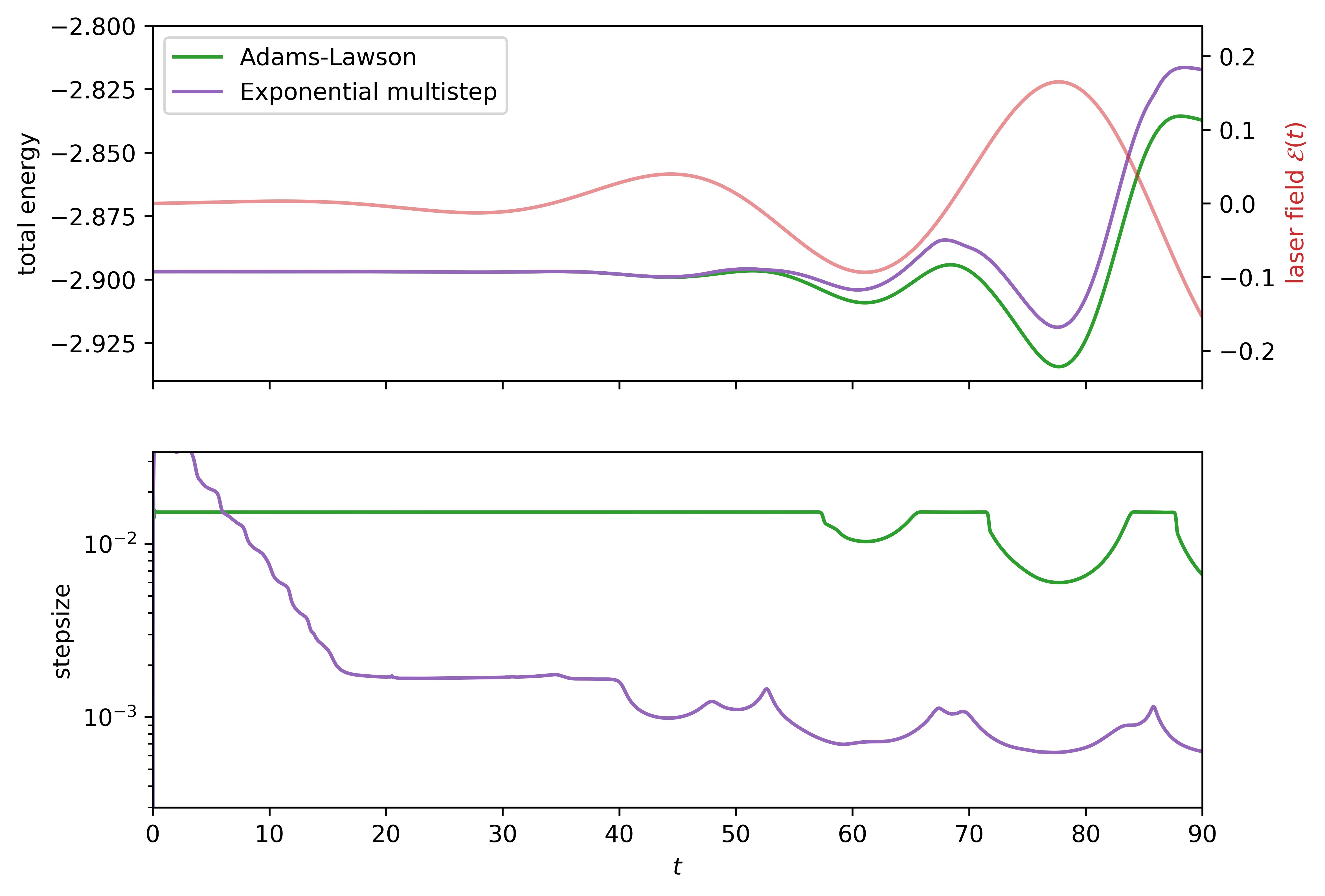
Figure 3: Total energy functional and external potential (top) and automatically generated stepsizes (bottom), MCTDHF with $N=4$.

References

- (1) Calvo, M., Palencia, C.: A class of explicit multistep exponential integrators for semilinear problems. Numer. Math. 102, 367–381 (2011)
- (2) Certaine, J.: The solution of ordinary differential equations with large time constants. In: Ralston, A., Wilf, H. (eds.) Mathematical Methods for Digital Computers, pp. 128–132. Wiley, Hoboken, N.J. (1960)
- (3) Frenkel, J.: Wave Mechanics, Advanced General Theory. Clarendon Press, Oxford (1934)
- (4) Friedli, A.: Verallgemeinerte Runge–Kutta Verfahren zur Lösung steifer Differentialgleichungssysteme. In: Bulirsch, R., Grigorieff, G., Schröder, J. (eds.) Numerical Treatment of Differential Equations, Lecture Notes in Mathematics, vol. 631, pp. 35–50. Springer (1978)
- (5) Hairer, E., Lubich, C., Wanner, G.: Geometric Numerical Integration. Springer-Verlag, Berlin–Heidelberg–New York (2002)
- (6) Hochbruck, M., Ostermann, A.: Exponential integrators. Acta Numer. 19, 209–286 (2010)
- (7) Hochbruck, M., Ostermann, A.: On the convergence of Lawson methods for semilinear stiff problems. CRC Preprint 2017/9, KIT Karlsruhe Institute of Technology (2017), https://www.waves.kit.edu/downloads/CRC1173_Preprint_2017-9.pdf
- (8) Koch, O.: Convergence of exponential Lawson-multistep methods for the MCTDHF equations, to appear in M2AN Math. Model. Numer. Anal.
- (9) Koch, O., Neuhauser, C., Thalhammer, M.: Error analysis of high-order splitting methods for nonlinear evolutionary Schrödinger equations and application to the MCTDHF equations in electron dynamics. M2AN Math. Model. Numer. Anal. 47, 1265–1284 (2013)
- (10) Lawson, J.: Generalized Runge–Kutta processes for stable systems with large Lipschitz constants. SIAM J. Numer. Anal. 4, 372––380 (1967)
- (11) Nørsett, S.: An A-stable modification of the Adams–Bashforth methods. In: Conference on the Numerical Solution of Differential Equations, Lecture Notes in Mathematics, vol. 109, pp. 214––219. Springer, Berlin–Heidelberg–New York (1969)
- (12) Zanghellini, J., Kitzler, M., Brabec, T., Scrinzi, A.: Testing the multi-configuration time-dependent Hartree-Fock method. J. Phys. B: At. Mol. Phys. 37, 763–773 (2004)