Coded Distributed Tracking

Abstract

We consider the problem of tracking the state of a process that evolves over time in a distributed setting, with multiple observers each observing parts of the state, which is a fundamental information processing problem with a wide range of applications. We propose a cloud-assisted scheme where the tracking is performed over the cloud. In particular, to provide timely and accurate updates, and alleviate the straggler problem of cloud computing, we propose a coded distributed computing approach where coded observations are distributed over multiple workers. The proposed scheme is based on a coded version of the Kalman filter that operates on data encoded with an erasure correcting code, such that the state can be estimated from partial updates computed by a subset of the workers. We apply the proposed scheme to the problem of tracking multiple vehicles. We show that replication achieves significantly higher accuracy than the corresponding uncoded scheme. The use of maximum distance separable (MDS) codes further improves accuracy for larger update intervals. In both cases, the proposed scheme approaches the accuracy of an ideal centralized scheme when the update interval is large enough. Finally, we observe a trade-off between age-of-information and estimation accuracy for MDS codes.

I Introduction

Tracking the state of a process that evolves over time in a distributed fashion is one of the most fundamental distributed information processing problems, with applications in, e.g., signal processing, control theory, robotics, and intelligent transportation systems (ITS) [1, 2, 3]. These applications typically require collecting data from multiple sources that is analyzed and acted upon in real-time, e.g., to track vehicles in ITS, and rely on timely status updates to operate effectively. The analysis and design of schemes for providing timely updates has received a significant interest in recent years. In a growing number of works, timeliness is measured by the age-of-information (AoI) [4], defined as the difference between the current time, $t$, and the largest generation time of a received message, $U(t)$, i.e., the AoI is $\Delta t=t-U(t)$.

Distributed tracking often entails highly demanding computational tasks. For example, in many previous works the computational complexity of the tasks performed by each node scales with the cube of the state dimension, see, e.g., [5, 2] and references therein. Thus, the proposed schemes are only suitable for low-dimensional processes. A notable exception is the algorithm proposed in [6], where the overall process is split into multiple overlapping subsystems to reduce the computational complexity. However, the algorithm in [6] is based on iterative message passing and potentially requires many iterations to reach consensus, which makes it difficult to provide timely updates.

Offloading computations over the cloud is an appealing solution to aggregate data and speed up demanding computations such that a stringent deadline is met. In [7], a cloud-assisted approach for autonomous driving was shown to significantly improve the response time compared to traditional systems, where vehicles are not connected to the cloud. However, servers in modern cloud computing systems rarely have fixed roles. Instead, incoming tasks are dynamically assigned to servers [8], which offers a high level of flexibility but also introduces significant challenges. For example, so-called straggling servers, i.e., servers that experience transient delays, may introduce significant delays [9]. Thus, for applications requiring very timely updates, offloading over the cloud must be done with care.

Recently, the use of erasure correcting codes has been proposed to alleviate the straggler problem in distributed computing systems [10, 11, 12]. In these works, redundancy is added to the computation such that the final output of the computation can later be decoded from a subset of the computed results. Hence, the delay is not limited by the slowest server.

In this paper, we consider a distributed tracking problem where multiple observers each observe parts of the state of the system, and their observations need to be aggregated to estimate the overall state [2, 6]. The goal is to provide timely and accurate information about the state of a stochastic process. An example is tracking vehicles to generate collision warning messages. We propose a cloud-assisted scheme where the tracking is performed over the cloud, which collects data from all observers. In particular, to speed up computations, the proposed scheme borrows ideas from coded distributed computing by distributing the observations over multiple workers, each computing one or more partial estimates of the state of the system. These partial estimates are finally merged at a monitor to produce an estimate of the overall state. To make the system robust against straggling servers, which may significantly impair the accuracy of the estimate unless accounted for, redundancy is introduced via the use of erasure correcting codes. In particular, the observations are encoded before they are distributed over the workers to increase the probability that the information is propagated to the monitor. A salient contribution of the paper is a coded filter based on the Kalman filter [1] that takes coded observations as its input and returns a state estimate encoded with an erasure correcting code. Hence, the monitor can obtain an overall estimate from a subset of the partial estimates via a decoding operation. We apply the proposed scheme to the problem of tracking multiple vehicles using repetition codes and random maximum distance separable (MDS) codes. We show that replication achieves significantly higher accuracy than the corresponding uncoded scheme and that MDS codes further improve accuracy for larger update intervals. Notably, both schemes approach the accuracy of an ideal centralized scheme for large enough update intervals. Finally, for MDS codes we observe a trade-off between AoI and accuracy, with update intervals shorter than some threshold leading to significantly lower accuracy.

II System Model and Preliminaries

We consider the problem of tracking the state of a stochastic process over time in a distributed setting. The state at time step $t$ is represented by a real-valued vector $\bm{x}_{t}$ of length $d$ and evolves over time according to

$$\bm{x}_{t}=\bm{F}\bm{x}_{t-1}+\bm{q}_{t},$$

where $\bm{F}$ is the matrix representing the state transition model and $\bm{q}_{t}$ is a noise vector drawn from a zero-mean Gaussian distribution with covariance matrix $\bm{Q}$. We denote by $\hat{\bm{x}}_{t}$ the state estimate at time $t$ and we measure the accuracy of the estimate by its root mean squared error (RMSE).

At each time step, a set of $N_{\mathsf{o}}$ observers, $\mathcal{O}=\{o_{1},\dots,o_{N_{\mathsf{o}}}\}$, obtain noisy partial observations of the state of the process. Specifically, the observation made by observer $o$ at time $t$ is represented by the vector

$$\bm{z}_{t}^{(o)}=\bm{H}^{(o)}\bm{x}_{t}+\bm{r}^{(o)}_{t},$$

where $\bm{H}^{(o)}$ is a matrix of size $h^{(o)}\times d$ representing the observation model of observer $o$ and $\bm{r}^{(o)}_{t}$ is a noise vector drawn from a zero-mean Gaussian distribution with covariance matrix $\bm{R}^{(o)}$. Furthermore, we denote by $\bm{z}_{t}$ the overall observation vector formed by concatenating the observations made by all observers, $\bm{z}_{t}^{(o_{1})},\dots,\bm{z}_{t}^{(o_{N_{\mathsf{o}}})}$, and by $h$ the length of $\bm{z}_{t}$. Similarly, we denote by $\bm{H}$ and $\bm{r}_{t}$ the overall observation model and noise vector, respectively, such that $\bm{z}_{t}=\bm{H}\bm{x}_{t}+\bm{r}_{t}$, and by $\bm{R}$ the covariance matrix of $\bm{r}_{t}$. For simplicity we assume that all observations are of equal dimension. We also assume that $h\geq d$ and that the entries of each observation $\bm{z}_{t}^{(o)}$ are linear combinations of a small number of entries of $\bm{x}_{t}$, i.e., the observation matrices $\bm{H}^{(o)}$ are sparse, as is the case, e.g., for an observer measuring speed. The observations made by the $N_{\mathsf{o}}$ observers need to be aggregated to estimate the overall state. Since $d$ may be large, the work of aggregating the observations is performed in the cloud over a set of $N_{\mathsf{w}}$ workers, $\mathcal{W}=\{w_{1},\dots,w_{N_{\mathsf{w}}}\}$. We assume that the matrices $\bm{F}$, $\bm{Q}$, $\bm{H}^{(o)}$, and $\bm{R}^{(o)}$ are known.

II-A Probabilistic Runtime Model

We assume that workers become unavailable for a random time after completing a computing task, which is captured by the exponential random variable $V$ with probability density function [10, 11]

$$f_{V}(v)=\begin{cases}\frac{1}{\beta}\mathrm{e}^{-\frac{v}{\beta}}&v\geq 0\\ 0&v<0\end{cases},$$

where $\beta$ is used to scale the tail of the distribution, which accounts for transient disturbances that are at the root of the straggler problem. We refer to $\beta$ as the straggling parameter.

II-B Distributed Tracking

At time step $t$, each observer $o$ uploads its observation $\bm{z}_{t}^{(o)}$ to the cloud, where the observations are encoded and distributed over the $N_{\mathsf{w}}$ workers. Next, each worker $w$ that becomes available during time step $t$ computes locally one or more partial estimates of the state $\bm{x}_{t}$. These partial estimates are forwarded to a monitor, which is responsible for computing the overall estimate of $\bm{x}_{t}$, denoted by $\hat{\bm{x}}_{t}$, from the partial estimates. Thus, the monitor has access to an updated state estimate at the end of each time step, which can be used for other applications (e.g., to generate collision warning messages in ITS). Finally, the overall estimate is sent back to the workers to be used in the next time step, i.e., we assume that all workers have access to $\hat{\bm{x}}_{t-1}$ at time step $t$.

II-C Kalman Filter

Denote by $\tilde{\bm{x}}_{t}$ the prediction of the state at time step $t$ based on the state estimate $\hat{\bm{x}}_{t-1}$ at time step $t-1$ and the state transition matrix $\bm{F}$, i.e., $\tilde{\bm{x}}_{t}=\bm{F}\hat{\bm{x}}_{t-1}$, and by $\tilde{\bm{P}}_{t}=\bm{F}\bm{P}_{t-1}\bm{F}^{\textup{{T}}}+\bm{Q}$ the covariance matrix of the error $\tilde{\bm{x}}_{t}-\bm{x}_{t}$, where $(\cdot)^{\textup{{T}}}$ denotes matrix transposition and $\bm{P}_{t-1}$ is the covariance matrix of the error $\hat{\bm{x}}_{t-1}-\bm{x}_{t-1}$ at time step $t-1$. The Kalman filter is an algorithm for combining the predicted state $\tilde{\bm{x}}_{t}$ with an observation $\bm{z}_{t}^{(o)}=\bm{H}^{(o)}\bm{x}_{t}+\bm{r}_{t}^{(o)}$ to produce an updated state estimate $\hat{\bm{x}}_{t}^{\prime}$ with minimum mean squared error [1]. Let $\tilde{\bm{y}}_{t}^{(o)}=\bm{z}_{t}^{(o)}-\bm{H}^{(o)}\tilde{\bm{x}}_{t}$ and denote by $\bm{S}_{t}^{(o)}=\bm{R}^{(o)}+\bm{H}^{(o)}\tilde{\bm{P}}_{t}\left(\bm{H}^{(o)}\right)^{\textup{{T}}}$ its covariance matrix. Then, the updated state estimate is $\hat{\bm{x}}_{t}^{\prime}=\tilde{\bm{x}}_{t}+\bm{K}_{t}^{(o)}\tilde{\bm{y}}_{t}^{(o)}$, where $\bm{K}_{t}^{(o)}=\tilde{\bm{P}}_{t}\left(\bm{H}^{(o)}\right)^{\textup{{T}}}\left(\bm{S}_{t}^{(o)}\right)^{-1}$ is the Kalman gain that determines how the observation should influence the updated estimate. The covariance matrix of the error $\hat{\bm{x}}_{t}^{\prime}-\bm{x}_{t}$ is $\bm{P}_{t}^{\prime}=\left(\bm{I}_{d}-\bm{K}_{t}^{(o)}\bm{H}^{(o)}\right)\tilde{\bm{P}}_{t}$, where $\bm{I}_{d}$ is the $d\times d$ identity matrix. If more than one observation is available, the estimate can be improved by setting $\tilde{\bm{x}}_{t}\leftarrow\hat{\bm{x}}_{t}^{\prime}$ and $\tilde{\bm{P}}_{t}\leftarrow\bm{P}_{t}^{\prime}$ and repeating this procedure. After repeating this procedure for all observations, the final estimate $\hat{\bm{x}}_{t}$ is obtained.

III Proposed Coded Scheme

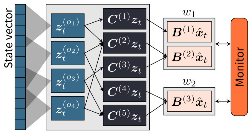
Figure 1: System overview example. Each of the $N_{\mathsf{o}}=4$ observers observes parts of the state, highlighted with a gray cone, and $N_{\mathsf{w}}=2$ workers compute $3$ coded state estimates from $5$ coded observations.

In this section, we introduce the proposed coded scheme. The key idea is the use of two layers of coding to make the system robust against straggling servers. The first layer consists of encoding the observations and distributing them over multiple workers. More specifically, the overall observation vector $\bm{z}_{t}$ is encoded by an $(n_{\mathsf{C}},h)$ linear erasure correcting code over the reals resulting in the vector $\bm{C}\bm{z}_{t}$, where $\bm{C}$ is a generator matrix of the code. Next, the elements of $\bm{C}\bm{z}_{t}$ are divided into $N_{\mathsf{C}}$ disjoint subvectors $\bm{C}^{(1)}\bm{z}_{t},\dots,\bm{C}^{(N_{\mathsf{C}})}\bm{z}_{t}$, where $\bm{C}^{(i)}$, $i=1,\dots,N_{\mathsf{C}}$, is the corresponding division of the rows of $\bm{C}$ into submatrices. We denote by $n_{\mathsf{C}}^{(i)}$ the number of rows of $\bm{C}^{(i)}$. For the rest of the paper we refer to $\bm{C}^{(i)}\bm{z}_{t}$ as a coded observation. This coding layer increases the probability that the information from an observation propagates to the monitor in case of delays.

The second layer of coding relates to the partial state estimates computed by each worker. Specifically, we propose a coded version of the Kalman filter that takes as its input the overall estimate at the previous time step $\hat{\bm{x}}_{t-1}$, provided by the monitor, one or more coded observations $\bm{C}^{(i)}\bm{z}_{t}$ from the current time step, and outputs a partial state estimate $\hat{\bm{x}}_{t}^{(j)}$. The proposed filter is such that the partial state estimate is equal to the estimate of the regular Kalman filter multiplied by some matrix $\bm{B}^{(j)}$. Equivalently, it can be seen as an estimate of the state of a process represented by the vector $\bm{B}^{(j)}\bm{x}_{t}$. Let $\bm{B}$ be a generator matrix of an $(n_{\mathsf{B}},d)$ linear erasure correcting code over the reals and let $\bm{B}^{(j)}$ be a submatrix of $\bm{B}$ of size $n_{\mathsf{B}}^{(j)}\times d$ such that $\bm{B}^{(1)},\dots,\bm{B}^{(N_{\mathsf{B}})}$ correspond to a division of the rows of $\bm{B}$ into $N_{\mathsf{B}}\leq N_{\mathsf{C}}$ disjoint submatrices. Hence, the partial estimates are symbols of the codeword $\bm{B}\hat{\bm{x}}_{t}$ and the monitor can recover the overall estimate $\hat{\bm{x}}_{t}$ from a subset of the partial estimates, ensuring that the monitor has access to timely and accurate estimates even if multiple workers experience delays.

Finally, we associate each coded state estimate $\bm{B}^{(j)}\hat{\bm{x}}_{t}$ with one worker and each coded observation $\bm{C}^{(i)}\bm{z}_{t}$ with one coded state estimate. We index the coded states associated with worker $w$ and the coded observations associated with $\bm{B}^{(j)}\hat{\bm{x}}_{t}$ with the sets $\mathcal{B}^{(w)}$ and $\mathcal{C}^{(j)}$, respectively. In total, worker $w$ receives the set $\{\bm{C}^{(i)}\bm{z}_{t}:i\in\bigcup_{j\in\mathcal{B}^{(w)}}\mathcal{C}^{(j)}\}$ of observations. The overall process is depicted in Fig. 1.

III-A Coded Update

When a worker $w$ becomes available it first computes the set $\{\bm{B}^{(j)}\hat{\bm{x}}_{t}:j\in\mathcal{B}^{(w)}\}$ of coded state estimates associated with it. The worker also computes a randomly selected subset of the Kalman gains associated with the uncoded filter, which will later be used by the monitor to approximate the covariance matrix $\bm{P}_{t}$. Each coded state estimate $\bm{B}^{(j)}\hat{\bm{x}}_{t}$ is computed from the previous state estimate $\hat{\bm{x}}_{t-1}$ and the set $\{\bm{C}^{(i)}\bm{z}_{t}:i\in\mathcal{C}^{(j)}\}$ of coded observations associated with it, and is computed independently from the other coded state estimates using the following procedure. First, the worker computes

$$\tilde{\bm{x}}_{t}^{(j)}=\left(\bm{B}^{(j)}\bm{F}\right)\hat{\bm{x}}_{t-1}$$

and the covariance matrix

$$\tilde{\bm{P}}_{t}^{(j)}=\left(\bm{B}^{(j)}\bm{F}\right)\bm{P}_{t-1}\left(\bm{B}^{(j)}\bm{F}\right)^{\textup{{T}}}+\bm{B}^{(j)}\bm{Q}\left(\bm{B}^{(j)}\right)^{\textup{{T}}}$$

of the error $\tilde{\bm{x}}_{t}^{(j)}-\bm{B}^{(j)}\bm{x}_{t}$. Next, $\tilde{\bm{x}}_{t}^{(j)}$ and $\tilde{\bm{P}}_{t}^{(j)}$ are combined with the associated observations, i.e., the observations in $\{\bm{C}^{(i)}\bm{z}_{t}:i\in\mathcal{C}^{(j)}\}$, one at a time, to produce $\hat{\bm{x}}_{t}^{(j)}$ and the covariance matrix $\bm{P}_{t}^{(j)}$ of the error $\hat{\bm{x}}_{t}^{(j)}-\bm{B}^{(j)}\bm{x}_{t}$ in the following way. First, consider a matrix $\bm{A}^{(i,j)}$ such that $\bm{A}^{(i,j)}\bm{B}^{(j)}=\bm{C}^{(i)}\bm{H}$. Then,

$$\begin{split}\bm{C}^{(i)}\bm{z}_{t}&=\bm{C}^{(i)}\left(\bm{H}\bm{x}_{t}+\bm{r}_{t}\right)\\ &=\bm{C}^{(i)}\bm{H}\bm{x}_{t}+\bm{C}^{(i)}\bm{r}_{t}\\ &=\bm{A}^{(i,j)}\bm{B}^{(j)}\bm{x}_{t}+\bm{C}^{(i)}\bm{r}_{t},\end{split}$$

i.e., the vector $\bm{C}^{(i)}\bm{z}_{t}$ can be considered as an observation of the state $\bm{B}^{(j)}\bm{x}_{t}$ with observation matrix $\bm{A}^{(i,j)}$ and observation noise covariance matrix $\bm{C}^{(i)}\bm{R}\left(\bm{C}^{(i)}\right)^{\textup{{T}}}$. Hence, using an observation $\bm{C}^{(i)}\bm{z}_{t}$, a partial coded state estimate $\hat{\bm{x}}_{t}^{\prime(j)}$ and the covariance matrix $\bm{P}_{t}^{\prime(j)}$ of the error $\hat{\bm{x}}_{t}^{\prime(j)}-\bm{B}^{(j)}\bm{x}_{t}$ can be obtained as

$$\hat{\bm{x}}_{t}^{\prime(j)}=\tilde{\bm{x}}_{t}^{(j)}+\bm{K}_{t}^{(i,j)}\tilde{\bm{y}}_{t}^{(i,j)},$$ (1)

$$\bm{P}_{t}^{\prime(j)}=\left(\bm{I}_{n_{\mathsf{B}}^{(j)}}-\bm{K}_{t}^{(i,j)}\bm{A}^{(i,j)}\right)\tilde{\bm{P}}_{t}^{(j)},$$ (2)

where

$$\tilde{\bm{y}}_{t}^{(i,j)}=\bm{C}^{(i)}\bm{z}_{t}-\bm{A}^{(i,j)}\tilde{\bm{x}}_{t}^{(j)},$$

$$\bm{K}_{t}^{(i,j)}=\tilde{\bm{P}}_{t}^{(j)}\left(\bm{A}^{(i,j)}\right)^{\textup{{T}}}\left(\bm{S}_{t}^{(i,j)}\right)^{-1},$$

$$\bm{S}_{t}^{(i,j)}=\bm{C}^{(i)}\bm{R}\left(\bm{C}^{(i)}\right)^{\textup{{T}}}+\bm{A}^{(i,j)}\tilde{\bm{P}}_{t}^{(j)}\left(\bm{A}^{(i,j)}\right)^{\textup{{T}}}.$$

Next, we let $\tilde{\bm{x}}_{t}^{(j)}\leftarrow\hat{\bm{x}}_{t}^{\prime(j)}$ and $\tilde{\bm{P}}_{t}^{(j)}\leftarrow\bm{P}_{t}^{\prime(j)}$ and repeat 1 and 2 for another observation until all observations in $\{\bm{C}^{(i)}\bm{z}_{t}:i\in\mathcal{C}^{(j)}\}$ have been used, at which point the coded state estimate $\hat{\bm{x}}_{t}^{(j)}$ has been computed. The covariance matrix $\bm{P}_{t}^{(j)}$ is only needed for computing $\hat{\bm{x}}_{t}^{(j)}$ and is discarded at this point. The worker repeats the above procedure for each coded state estimate $\hat{\bm{x}}_{t}^{(j)}$, $j\in\mathcal{B}^{(w)}$, assigned to it. Once finished, the worker separately computes the Kalman gain of the uncoded filter $\bm{K}_{t}^{(o)}$, as explained in Section II-C, associated with some number $N_{\mathsf{K}}$ of observers $o$ selected uniformly at random from $\mathcal{O}$. Finally, the coded state estimates are sent to the monitor together with the $\bm{K}_{t}^{(i,j)}$ and $\bm{S}_{t}^{(i,j)}$ matrices and the uncoded Kalman gains computed by the worker, where they are used to recover the overall state estimate $\hat{\bm{x}}_{t}$ and the error covariance matrix $\bm{P}_{t}$.

III-B Decoding

At the end of each time step $t$ the monitor attempts to recover $\hat{\bm{x}}_{t}$ from the partial coded state estimates $\hat{\bm{x}}_{t}^{(j)}$ received from the workers. This corresponds to a decoding operation. Denote by $\mathcal{U}_{t}$ the set of coded state estimates the monitor receives at time step $t$ and by $\bm{B}_{\hat{\bm{x}}_{t}}$ the vertical concatenation of the generator matrices associated with those estimates. To decode, the monitor needs to solve for $\hat{\bm{x}}_{t}$ in $\bm{B}_{\hat{\bm{x}}_{t}}\hat{\bm{x}}_{t}=\bm{y}_{\hat{\bm{x}}_{t}}$, where $\bm{y}_{\hat{\bm{x}}_{t}}$ is the vertical concatenation of the vectors $\hat{\bm{x}}_{t}^{(j)}$ in $\mathcal{U}_{t}$. However, there are two issues that need to be addressed before solving for $\hat{\bm{x}}_{t}$. First, due to the dependence structure of the tracking problem and the coding introduced, the elements of $\bm{y}_{\hat{\bm{x}}_{t}}$ will in general be correlated and have varying variance, which must be accounted for to recover $\hat{\bm{x}}_{t}$ optimally. Second, since the local estimates by the workers are noisy, $\bm{B}_{\hat{\bm{x}}_{t}}\hat{\bm{x}}_{t}=\bm{y}_{\hat{\bm{x}}_{t}}$ typically does not have an exact solution. We address the first issue by applying a so-called whitening transform to the original problem, i.e., we solve for $\hat{\bm{x}}_{t}$ in $\bm{M}_{\hat{\bm{x}}_{t}}\bm{B}_{\hat{\bm{x}}_{t}}\hat{\bm{x}}_{t}=\bm{M}_{\hat{\bm{x}}_{t}}\bm{y}_{\hat{\bm{x}}_{t}}$, where $\bm{M}_{\hat{\bm{x}}_{t}}$ is a linear transform that has the effect of uncorrelating and normalizing the variance of the elements of $\bm{y}_{\hat{\bm{x}}_{t}}$. The whitening transform $\bm{M}_{\hat{\bm{x}}_{t}}$ is computed from the singular value decomposition of the covariance matrix of $\bm{y}_{\hat{\bm{x}}_{t}}$, which we denote by $\bm{P}_{\hat{\bm{x}}_{t}}$, as in [13]. The covariance matrix $\bm{P}_{\hat{\bm{x}}_{t}}$ is given by [14, Eq. (6.47)], where the covariance matrix, Kalman gain, observation model, and observation noise covariance matrix of the uncoded filter update procedure are replaced by their coded equivalents from Section III-A. We address the second issue by finding the vector $\hat{\bm{x}}_{t}$ that minimizes the $\ell_{2}$-norm of the error, i.e., by solving $\operatorname*{arg\,min}_{\hat{\bm{x}}_{t}}{||\bm{M}_{\hat{\bm{x}}_{t}}\bm{B}_{\hat{\bm{x}}_{t}}\hat{\bm{x}}_{t}-\bm{M}_{\hat{\bm{x}}_{t}}\bm{y}_{\hat{\bm{x}}_{t}}||}_{2}$. We achieve this by decoding $\hat{\bm{x}}_{t}$ using the LSMR algorithm [15]. The LSMR algorithm is a numerical procedure for solving problems of this type that takes an initial guess of the solution as its input and iteratively improves on the solution until it has converged to within some threshold. We give $\tilde{\bm{x}}_{t}$, which the monitor computes from $\hat{\bm{x}}_{t-1}$ as explained in Section II-C, as the initial guess since the Euclidean distance between $\hat{\bm{x}}_{t}$ and $\tilde{\bm{x}}_{t}$ typically is small.

Next, the monitor approximates the error covariance matrix $\bm{P}_{t}$ using the following heuristic. First, the monitor computes $\tilde{\bm{P}}_{t}$ from $\bm{P}_{t-1}$ as explained in Section II-C. Denote by $r$ the maximum rank of $\bm{P}_{\hat{\bm{x}}_{t}}$, i.e., the rank of $\bm{P}_{\hat{\bm{x}}_{t}}$ when all workers are available, and by $r_{\hat{\bm{x}}_{t}}$ the rank of the given $\bm{P}_{\hat{\bm{x}}_{t}}$. Now, if $r_{\hat{\bm{x}}_{t}}<r$ we assume that the monitor has insufficient information to recover $\hat{\bm{x}}_{t}$ optimally and we let $\bm{P}_{t}=\tilde{\bm{P}}_{t}$. On the other hand, if $r_{\hat{\bm{x}}_{t}}=r$, we assume that the monitor has recovered $\hat{\bm{x}}_{t}$ optimally, and the monitor computes $\bm{P}_{t}$ from $\tilde{\bm{P}}_{t}$ using the procedure for a full update of the uncoded filter (see Section II-C). More formally, denote by $\bm{K}_{t_{o}}^{(o)}$ the most recently received Kalman gain corresponding to observer $o$ at time step $t_{o}$. Then, the monitor computes $\bm{P}_{t}^{\prime}=\left(\bm{I}_{d}-\bm{K}_{t_{o}}^{(o)}\bm{H}^{(o)}\right)\tilde{\bm{P}}_{t}$, assigns $\tilde{\bm{P}}_{t}\leftarrow\bm{P}_{t}^{\prime}$, and repeats the procedure for each remaining observer $o\in\mathcal{O}$. Finally, we let $\bm{P}_{t}\leftarrow\tilde{\bm{P}}_{t}$. Note that $\bm{P}_{t}$ depends only on the statistical properties of the observations, i.e., it can be computed without access to the observations themselves.

IV Design and Analysis of the Proposed Scheme

We analyze the computational complexity of the proposed coded scheme, design the generator matrices required for the coded filter update, and choose how the computations are distributed over the workers.

IV-A Computational Complexity

We assume that the number of arithmetic operations performed by the workers is dominated by the number of operations needed to invert $\bm{S}$ when computing the Kalman gain, which requires in the order of $n^{3}$ operations, where $n$ is the number of rows and columns of $\bm{S}$. Since each worker computes $N_{\mathsf{K}}$ Kalman gains associated with the uncoded filter in addition to those needed for the coded state estimates, and due to our assumption that all uncoded observations have equal dimension, the overall number of operations performed by the workers can be approximated by $N_{\mathsf{K}}N_{\mathsf{w}}\left(h^{(o)}\right)^{3}+\sum_{w\in\mathcal{W}}\sum_{j\in\mathcal{B}^{(w)}}\sum_{i\in\mathcal{C}^{(j)}}\left(n_{\mathsf{C}}^{(i)}\right)^{3}$.

IV-B Code Design

Here, we propose two strategies for designing the sets $\mathcal{B}^{(w)}$ and $\mathcal{C}^{(j)}$ and the matrices $\bm{B}^{(1)},\dots,\bm{B}^{(N_{\mathsf{B}})}$ and $\bm{C}^{(1)},\dots,\bm{C}^{(N_{\mathsf{C}})}$. The matrices $\bm{A}^{(i,j)}$ are determined implicitly since $\bm{A}^{(i,j)}\bm{B}^{(j)}=\bm{C}^{(i)}\bm{H}$. The first design is based on replication, which is a special case of MDS codes, whereas the second is based on random MDS codes.

IV-B1 Replication

This design is based on replicating the tracking task at each worker, i.e., the code rate is $h/n_{\mathsf{C}}=1/N_{\mathsf{w}}$. More formally, each worker estimates $\bm{x}_{t}$, i.e., $N_{\mathsf{B}}=N_{\mathsf{w}}$, $\bm{B}^{(j)}=\bm{I}_{d}$, $j=1,\dots,N_{\mathsf{B}}$, $\mathcal{B}^{(w_{1})}=\{1\},\dots,\mathcal{B}^{(w_{N_{\mathsf{B}}})}=\{N_{\mathsf{B}}\}$, and each state estimate is computed from the full set of observations, i.e., $N_{\mathsf{C}}=N_{\mathsf{w}}N_{\mathsf{o}}$ and the observation encoding matrices and sets $\mathcal{C}^{(j)}$ associated with each estimate $\hat{\bm{x}}_{t}^{(j)}=\hat{\bm{x}}_{t}$ are such that $\{\bm{C}^{(i)}\bm{z}_{t}:i\in\mathcal{C}^{(j)}\}=\{\bm{z}_{t}^{(o)}:o\in\mathcal{O}\}$. Note that the monitor can recover $\hat{\bm{x}}_{t}$ and $\bm{P}_{t}$ immediately upon receiving these values from any worker without performing any additional computations. Hence, we let $N_{\mathsf{K}}=0$ and the overall number of operations performed by the workers is approximately $\frac{N_{\mathsf{o}}}{(h/n_{\mathsf{C}})}\left(h^{(o)}\right)^{3}$.

IV-B2 Random MDS Coding

This design is based on assigning a large number of coded state estimates of dimension one to each worker, i.e., we let $n_{\mathsf{B}}^{(j)}=1$, $j=1,\dots,N_{\mathsf{B}}$. Furthermore, to ensure that the code is well-conditioned, i.e., the numerical precision lost due to the coding is low, we generate $\bm{C}$ by drawing each element independently at random from a standard Gaussian distribution [16]. To satisfy the requirement $\bm{A}^{(i,j)}\bm{B}^{(j)}=\bm{C}^{(i)}\bm{H}$ we let $\bm{B}^{(j)}=\bm{C}^{(i)}\bm{H}$ and $\bm{A}^{(i,j)}=\bm{I}_{1}$. As a result, $n_{\mathsf{C}}^{(i)}=1$, $i=1,\dots,N_{\mathsf{C}}$, and we associate each observation one-to-one with a coded state estimate, i.e., $N_{\mathsf{B}}=N_{\mathsf{C}}$ and $\mathcal{C}^{(1)}=\{1\},\dots,\mathcal{C}^{(N_{\mathsf{B}})}=\{N_{\mathsf{B}}\}$. Next, we split the coded state estimates as evenly as possible over the $N_{\mathsf{w}}$ workers, i.e., some workers are assigned $\lfloor N_{\mathsf{B}}/N_{\mathsf{w}}\rfloor$ estimates and some are assigned $\lceil N_{\mathsf{B}}/N_{\mathsf{w}}\rceil$ estimates. Finally, we let $N_{\mathsf{K}}=\left\lceil\frac{N_{\mathsf{o}}/(h/n_{\mathsf{C}})}{N_{\mathsf{w}}}\right\rceil$, which, since $n_{\mathsf{C}}^{(i)}=1$, $i=1,\dots,N_{\mathsf{C}}$, means that the overall number of operations performed by the workers is approximately $\frac{N_{\mathsf{o}}}{(h/n_{\mathsf{C}})}\left(h^{(o)}\right)^{3}$.

V Numerical Results

To evaluate the performance of the proposed scheme, we consider a distributed vehicle tracking scenario where $N_{\mathsf{w}}$ workers cooperate to track the position of $N_{\mathsf{v}}$ vehicles $v_{1},\dots,v_{N_{\mathsf{v}}}$ based on observations received from the vehicles. We model the state of each vehicle with a length-$4$ vector composed of its position and speed in the longitudinal and latitudinal directions, i.e., the overall state dimension is $d=4N_{\mathsf{v}}$. As in [17], we assume that the state transition matrix of a single vehicle is

$$\bm{F}_{\mathsf{v}}=\begin{bmatrix}1&0&\Delta t&0\\ 0&1&0&\Delta t\\ 0&0&1&0\\ 0&0&0&1\end{bmatrix}$$

and that the associated covariance matrix is

$$\bm{Q}_{\mathsf{v}}=\bm{V}\begin{bmatrix}\sigma_{\mathsf{a}}&0\\ 0&\sigma_{\mathsf{a}}\end{bmatrix}\bm{V}^{\textup{{T}}},\;\;\text{with}\;\;\bm{V}=\begin{bmatrix}\Delta t^{2}/2&0\\ 0&\Delta t^{2}/2\\ \Delta t&0\\ 0&\Delta t\end{bmatrix}.$$

Hence, the combined state transition matrix and covariance matrix for all vehicles is $\bm{F}=\bm{I}_{N_{\mathsf{v}}}\otimes\bm{F}_{\mathsf{v}}$ and $\bm{Q}=\bm{I}_{N_{\mathsf{v}}}\otimes\bm{Q}_{\mathsf{v}}$, respectively. We assume that each vehicle observes its absolute position, e.g., using global navigation satellite systems (GNSSs), and speed in the longitudinal and latitudinal directions. The corresponding observation matrix is $\bm{H}_{\mathsf{v}}=\bm{I}_{4}$, with associated covariance matrix $\bm{R}_{\mathsf{GNSS}}=\text{diag}(\sigma_{\mathsf{GNSS}}^{2},\sigma_{\mathsf{GNSS}}^{2},\sigma_{\mathsf{speed}}^{2},\sigma_{\mathsf{speed}}^{2})$, where $\text{diag}(\cdot)$ denotes the diagonal, or block-diagonal, matrix composed of the arguments of $\text{diag}(\cdot)$ arranged along the diagonal. Furthermore, similar to [17] we assume that each vehicle observes the distance and speed difference in the longitudinal and latitudinal directions relative to a number $s<N_{\mathsf{v}}$ of other vehicles using, e.g., radar or lidar. By combining these observations in a cooperative manner the accuracy of the vehicle position estimates can be improved compared to a system relying only on GNSS observations. The covariance matrix associated with a relative observation is $\bm{R}_{\mathsf{Rel.}}=\text{diag}(\sigma_{\mathsf{V2V}}^{2},\sigma_{\mathsf{V2V}}^{2},\sigma_{\mathsf{speed}}^{2},\sigma_{\mathsf{speed}}^{2})$.

For each vehicle $v_{i}$, define the matrix $\bm{U}^{(v_{i})}$ of size $(s+1)\times N_{\mathsf{v}}$, where the first row corresponds to the absolute observation of the vehicle and each of the $s$ remaining rows correspond to an observation relative to another vehicle. The $i$-th column of $\bm{U}^{(v_{i})}$ has $s+1$ nonzero entries and the remaining columns each have exactly one nonzero entry. For the first row of $\bm{U}^{(v_{i})}$ the $i$-th entry has value $1$, while the remaining entries have value $0$. For each of the remaining rows the $i$-th entry has value $-1$ and one other entry corresponding to the observed vehicle has value $1$. For example, if $s=2$ and vehicle $v_{i}$ can observe vehicles $v_{j}$ and $v_{k}$ the second and third row will have value $1$ in column $j$ and $k$, respectively. Then, the observation matrix for vehicle $v_{i}$ is $\bm{H}^{(v_{i})}=\bm{U}^{(v_{i})}\otimes\bm{H}_{\mathsf{v}}$. The corresponding observation noise covariance matrix is $\text{diag}\left(\bm{R}_{\mathsf{GNSS}},\bm{I}_{s}\otimes\bm{R}_{\mathsf{Rel.}}\right)$. Finally, $\bm{U}^{(v_{i})}$ is generated for one vehicle at a time such that the first vehicle observes vehicles $v_{2},\dots,v_{s+1}$, and, in general, vehicle $v_{i}$ observes vehicles $v_{(j\bmod N_{\mathsf{v}})+1}$, $j=i,\dots,i+s-1$.

We compare the performance of the proposed scheme with that of an ideal centralized scheme where the monitor has unlimited processing capacity and processes all observations itself using the procedure in Section II-C. We also compare against the performance of an uncoded scheme, where each observation is processed by a single worker with no coding. More formally, we divide the $N_{\mathsf{o}}$ observations as evenly as possible over the $N_{\mathsf{w}}$ workers, assigning $\lfloor N_{\mathsf{o}}/N_{\mathsf{w}}\rfloor$ observations to some workers and $\lceil N_{\mathsf{o}}/N_{\mathsf{w}}\rceil$ observations to the remaining workers. Next, each worker estimates $\bm{x}_{t}$ using the uncoded update procedure given in Section II-C. For this scheme, the monitor estimate is equal to the average of the estimates received from the workers at each time step, i.e., $\hat{\bm{x}}_{t}$ is the average of the estimates in $\mathcal{U}_{t}$ and $\bm{P}_{t}$ is the average of the corresponding covariance matrices.

We consider the vehicle tracking problem described above with $\sigma_{\mathsf{a}}=0.3$, $\sigma_{\mathsf{GNSS}}=2$, $\sigma_{\mathsf{V2V}}=0.5$, and $\sigma_{\mathsf{speed}}=10$. For all schemes, we run $10$ simulations, each of $T=10000$ time steps, and compute the RMSE of the position estimate at each time step. More specifically, we denote by $\bm{x}_{\mathsf{p},t}$ and $\hat{\bm{x}}_{\mathsf{p},t}$ the vectors composed of the entries of $\bm{x}_{t}$ and $\hat{\bm{x}}_{t}$ corresponding to position, e.g., entries $1,2,5,6$ if $N_{\mathsf{v}}=2$, and compute $m_{t}\triangleq\sqrt{\frac{1}{d/2}\bm{e}_{\mathsf{p},t}\bm{e}_{\mathsf{p},t}^{\textup{{T}}}}$, where $\bm{e}_{\mathsf{p},t}=\hat{\bm{x}}_{\mathsf{p},t}-\bm{x}_{\mathsf{p},t}$, for $t=1,\dots,T$. Next, for each simulation, to avoid any initial transients, we discard the first $t_{0}-1$ samples $m_{1},\dots,m_{t_{0}-1}$. We let $t_{0}$ be the smallest value such that

$$\frac{|\bar{m}_{t_{0}:t_{\mathsf{m}}}-\bar{m}_{(t_{\mathsf{m}}+1):T}|}{\max\left(\bar{m}_{t_{0}:t_{\mathsf{m}}},\bar{m}_{(t_{\mathsf{m}}+1):T}\right)}\leq 0.1,$$

where $t_{\mathsf{m}}=t_{0}+\lfloor(T-t_{0})/2\rfloor$ and $\bar{m}_{t_{1}:t_{2}}$ denotes the mean of $m_{t_{1}},\dots,m_{t_{2}}$. Finally, we plot the $90$-th percentile of the RMSE of the position estimate over the concatenation of the remaining samples from all simulations.

In Fig. 2, we show the $90$-th percentile of the RMSE of the position as a function of the update interval $\Delta t$ for replication and random MDS codes with rates $1/2$ and $1/3$. For replication the code rate is $h/n_{\mathsf{C}}=1/N_{\mathsf{w}}$ (see Section IV-B), i.e., the number of workers is $N_{\mathsf{w}}=2$ and $N_{\mathsf{w}}=3$ for rates $1/2$ and $1/3$, respectively. MDS codes support an arbitrary number of workers and we let $N_{\mathsf{w}}=16$ for this design. We show the RMSE for $0.01\leq\Delta t\leq 0.25$ since several applications in ITS require an AoI in this range [3]. There are $N_{\mathsf{v}}=10$ vehicles, each observing $s=5$ other vehicles, and the straggling parameter is $\beta=10$, i.e., workers become unavailable for $0.1$ seconds on average after a filter update. Here, replication improves accuracy significantly compared to the uncoded scheme, with a $90$-th percentile RMSE of about $0.27$ and $0.25$ meters for code rates $1/2$ and $1/3$, respectively, when $\Delta t=0.1$. MDS codes improve the accuracy further at this point, with about a $2.4$% and $5.5$% smaller error when compared at code rates $1/2$ and $1/3$, respectively. Finally, for MDS codes we observe a trade-off between AoI and accuracy, with update intervals shorter than some threshold, e.g., $\Delta t=0.05$ for code rate $1/3$, leading to a higher RMSE since the probability of the monitor collecting enough coded state estimates to decode $\hat{\bm{x}}_{t}$ approaches zero when $\Delta t\to 0$.

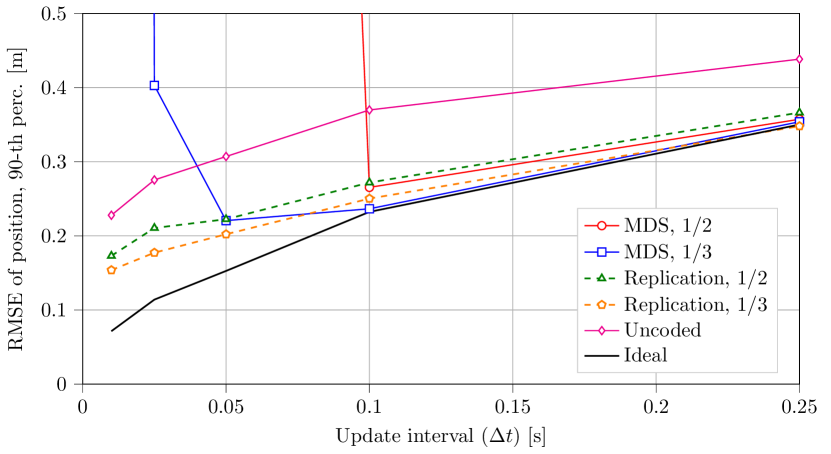
Figure 2: $90$-th percentile of the RMSE of the position over $10$ simulations, each of $T=10000$ samples, as a function of $\Delta t$ for $N_{\mathsf{v}}=10$, $s=5$, $N_{\mathsf{w}}=16$ (for MDS codes), and $\beta=10$.

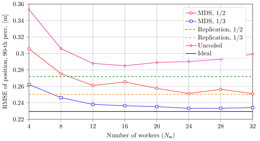
Figure 3: $90$-th percentile of the RMSE of the position over $10$ simulations, each of $T=10000$ samples, as a function of $N_{\mathsf{w}}$ for $N_{\mathsf{v}}=10$, $s=5$, $\Delta t=0.1$, and $\beta=10$.

In Fig. 3, we show the $90$-th percentile of the RMSE of the position for random MDS codes as a function of the number of workers $N_{\mathsf{w}}$ for $N_{\mathsf{v}}=10$ vehicles, each observing $s=5$ other vehicles, $\Delta t=0.1$, and $\beta=10$. We also show the error of replication (with $N_{\mathsf{w}}$ fixed to $2$ and $3$ for code rates $1/2$ and $1/3$, respectively) and the uncoded and ideal schemes. The accuracy of the design based on MDS codes generally improves with $N_{\mathsf{w}}$, since the variance of the fraction of workers available in each time step decreases. In some cases, e.g., for code rate $1/2$ and $N_{\mathsf{w}}=28$, the error increases since the fraction of servers needed to decode $\hat{\bm{x}}_{t}$ may increase if the number of coded state estimates does not divide evenly over the workers. Here, the error of MDS codes is lower than that of replication when $N_{\mathsf{w}}\geq 12$ and $N_{\mathsf{w}}\geq 8$ for code rates $1/2$ and $1/3$, respectively. We also observe that the performance does not improve significantly beyond some number of workers.

VI Conclusion

We presented a novel scheme for tracking the state of a process in a distributed setting, which we refer to as coded distributed tracking. The proposed scheme extends the idea of coded distributed computing to the tracking problem by considering a coded version of the Kalman filter, where observations are encoded and distributed over multiple workers, each computing partial state estimates encoded with an erasure correcting code, which alleviates the straggler problem since missing results can be compensated for. The proposed coded schemes achieves significantly higher accuracy than the uncoded scheme and approaches the accuracy of an ideal centralized scheme when the update interval is large enough. We believe that coded distributed tracking can be a powerful alternative to previously proposed approaches.

References

- [1] R. E. Kalman, “A new approach to linear filtering and prediction problems,” Trans. ASME J. Basic Eng., vol. 82, no. 1, pp. 35–45, Mar. 1960.
- [2] R. Olfati-Saber, “Distributed Kalman filtering for sensor networks,” in Proc. IEEE Conf. Decision Control (CDC), New Orleans, LA, 2007.
- [3] P. Papadimitratos, A. de La Fortelle, K. Evenssen, R. Brignolo, and S. Cosenza, “Vehicular communication systems: Enabling technologies, applications, and future outlook on intelligent transportation,” IEEE Commun. Mag., vol. 47, no. 11, pp. 84–95, Nov. 2009.
- [4] R. D. Yates and S. Kaul, “Real-time status updating: Multiple sources,” in Proc. IEEE Int. Symp. Inf. Theory (ISIT), Cambridge, MA, 2012.
- [5] M. S. Mahmoud and H. M. Khalid, “Distributed Kalman filtering: a bibliographic review,” IET Control Theory Appl., vol. 7, no. 4, pp. 483–501, Mar. 2013.
- [6] U. A. Khan and J. M. F. Moura, “Distributing the Kalman filter for large-scale systems,” IEEE Trans. Signal Process., vol. 56, no. 10, pp. 4919–4935, Oct. 2008.
- [7] S. Kumar, S. Gollakota, and D. Katabi, “A cloud-assisted design for autonomous driving,” in Proc. Workshop Mobile Cloud Comput. (MCC), Helsinki, Finland, 2012.
- [8] A. Verma, L. Pedrosa, M. Korupolu, D. Oppenheimer, E. Tune, and J. Wilkes, “Large-scale cluster management at Google with Borg,” in Proc. Eur. Conf. Computer Syst. (EuroSys), Bordeaux, France, 2015.
- [9] J. Dean and S. Ghemawat, “MapReduce: Simplified data processing on large clusters,” in Proc. Symp. Oper. Syst. Design Implement. (OSDI), San Francisco, CA, 2004.
- [10] S. Li, M. A. Maddah-Ali, and A. S. Avestimehr, “A unified coding framework for distributed computing with straggling servers,” in Proc. Workshop Network Coding Appl. (NetCod), Washington, DC, 2016.
- [11] K. Lee, M. Lam, R. Pedarsani, D. Papailiopoulos, and K. Ramchandran, “Speeding up distributed machine learning using codes,” IEEE Trans. Inf. Theory, vol. 64, no. 3, pp. 1514–1529, Mar. 2018.
- [12] A. Severinson, A. Graell i Amat, and E. Rosnes, “Block-diagonal and LT codes for distributed computing with straggling servers,” IEEE Trans. Commun., vol. 67, no. 3, pp. 1739–1753, Mar. 2019.
- [13] A. Kessy, A. Lewin, and K. Strimmer, “Optimal whitening and decorrelation,” The American Stat., vol. 72, no. 4, pp. 309–314, Nov. 2018.
- [14] S. Polavarapu, “The Kalman filter,” Dept. of Physics, University of Toronto, Toronto, ON, Canada, Tech. Rep., 2004. [Online]. Available: http://www.atmosp.physics.utoronto.ca/PHY2509/ch6.pdf
- [15] D. C.-L. Fong and M. Saunders, “LSMR: An iterative algorithm for sparse least-squares problems,” SIAM J. Sci. Comput., vol. 33, no. 5, pp. 2950–2971, Oct. 2011.
- [16] Z. Chen and J. Dongarra, “Numerically stable real number codes based on random matrices,” in Proc. Int. Conf. Comput. Sci. (ICCS), Atlanta, GA, 2005.
- [17] G. Soatti, M. Nicoli, N. Garcia, B. Denis, R. Raulefs, and H. Wymeersch, “Implicit cooperative positioning in vehicular networks,” IEEE Trans. Intell. Transp. Syst., vol. 19, no. 12, pp. 3964–3980, Dec. 2018.