Imputing Missing Events in Continuous-Time Event Streams

Abstract

Events in the world may be caused by other, unobserved events. We consider sequences of events in continuous time. Given a probability model of complete sequences, we propose particle smoothing—a form of sequential importance sampling—to impute the missing events in an incomplete sequence. We develop a trainable family of proposal distributions based on a type of bidirectional continuous-time LSTM: Bidirectionality lets the proposals condition on future observations, not just on the past as in particle filtering. Our method can sample an ensemble of possible complete sequences (particles), from which we form a single consensus prediction that has low Bayes risk under our chosen loss metric. We experiment in multiple synthetic and real domains, using different missingness mechanisms, and modeling the complete sequences in each domain with a neural Hawkes process (Mei & Eisner, 2017). On held-out incomplete sequences, our method is effective at inferring the ground-truth unobserved events, with particle smoothing consistently improving upon particle filtering.

[1] [2]if #1 : #2 [3]if #1 : #2 else #3 {}[1] $\triangleright$ #1 [1]$\triangleright$ #1 [1]$\triangleright$ #1 inputInput: outputOutput: [1] #1

1 Introduction

Event streams of discrete events in continuous time are often partially observed. We would like to impute the missing events ${\bm{\mathbf{z}}}$. Suppose we know the prior distribution $p_{\text{model}}$ of complete event streams, as well as the “missingness mechanism” $p_{\text{miss}}({\bm{\mathbf{z}}}\mid\text{complete stream})$, which stochastically determines which of the events will not be observed. One can then use use Bayes’ Theorem, as spelled out in equation 1 below, to define the posterior distribution $p({\bm{\mathbf{z}}}\mid{\bm{\mathbf{x}}})$ given just the observed events ${\bm{\mathbf{x}}}$.

Figure 1: Stochastically imputing a taxi’s pick-up events ( ) given its observed drop-off events ( ). At this stage, we are trying to determine the next event after the at time $t_{1}$—either an unobserved event at $t_{1,1}\in(t_{1},t_{2})$ or the next observed event at $t_{2}$.

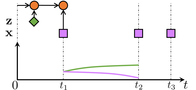
a1 Both intensities are low (i.e., passengers are scarce at this time of day), so no event happens to be proposed in $(t_{1},t_{2})$.

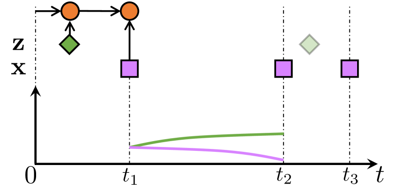
a2 Specifically, the next proposed event ( ) would be somewhere after $t_{2}$, without bothering to determine its time precisely.

a3 Thus, the next event is $\leavevmode\hbox to5.64pt{\vbox to5.64pt{\text{[drawing]}}}{\scriptstyle@}t_{2}$; we feed it into the LSTM, preempting , which is discarded (LABEL:line:preempt of Algorithm 1).

(a) Particle filtering (section 3.1). We show part of the process of drawing one particle. Above left, the neural Hawkes process’s LSTM has already read the proposed and observed events at times $\leq t_{1}$. Its resulting state determines the model intensities and of the two event types and , from which the sampler (Algorithm 1 in Appendix C) determines that there is no unobserved event in $(t_{1},t_{2})$. Above right, we continue to extend the particle by feeding $\leavevmode\hbox to5.64pt{\vbox to5.64pt{\text{[drawing]}}}{\scriptstyle@}t_{2}$ into the LSTM and proposing subsequent events based on the new intensities after $t_{2}$. But because was low at $t_{2}$, the $\leavevmode\hbox to5.64pt{\vbox to5.64pt{\text{[drawing]}}}{\scriptstyle@}t_{2}$ was unexpected, and that results in downweighting the particle (LABEL:line:downweight of Algorithm 1). Downweighting recognizes belatedly that proposing no event in $(t_{1},t_{2})$ has committed us to a particle that will be improbable under the posterior, because its complete sequence includes consecutive drop-offs ($\leavevmode\hbox to5.64pt{\vbox to5.64pt{\text{[drawing]}}}{\scriptstyle@}t_{1},\leavevmode\hbox to5.64pt{\vbox to5.64pt{\text{[drawing]}}}{\scriptstyle@}t_{2}$) far apart in time.

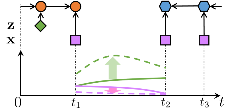
b1 Since a drop-off at $t_{2}$ strongly suggests a pick-up before $t_{2}$, considering the future increases the intensity of pick-up on $(t_{1},t_{2})$ from to (while decreasing that of drop-off from to ).

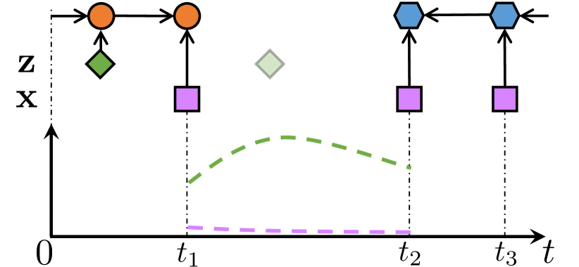
b2 Consequently, the next proposed event is more likely to be a pick-up in $(t_{1},t_{2})$ than it was in Figure 1(a). If we stochastically generate such an event $\leavevmode\hbox to6.84pt{\vbox to6.84pt{\text{[drawing]}}}{\scriptstyle@}t_{1,1}$, it is fed into the original LSTM.

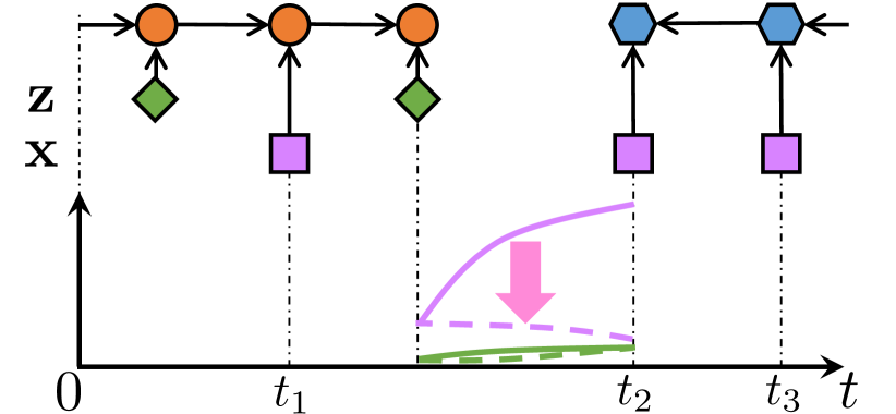
b3 The updated state determines the new model intensities and , and also combines with to determine the new proposal intensities and , which are used to sample the next event.

(b) Particle smoothing (section 3.2) samples from a better-informed proposal distribution: a second LSTM (LABEL:sec:r2l) reads the future observations from right to left, and its state is used together with to determine the proposal intensities and .

Why is this important?

The ability to impute ${\bm{\mathbf{z}}}$ is useful in many applied domains, for example:

• Medical records. Some patients record detailed symptoms, self-administered medications, diet, and sleep. Imputing these events for other patients would produce an augmented medical record that could improve diagnosis, prognosis, treatment, and counseling.

  Similar remarks apply to users of life-tracking apps (e.g., MyFitnessPal) who forget to log some of their daily activities (e.g., meals, sleep and exercise).

• Competitive games. In poker or StarCraft, a player lacks full information about what her opponents have acquired (cards) or done (build mines and train soldiers). Accurately imputing hidden actions from “what I did” and “what I observed others doing” can help the player make good decisions. Similar remarks apply to practical scenarios (e.g., military) where multiple actors compete and/or cooperate.

• User interface interactions. Cognitive events are usually unobserved. For example, users of an online news provider (e.g., Bloomberg Terminal) may have read and remembered a displayed headline whether or not they clicked on it. Such events are expensive to observe (e.g., via gaze tracking or asking the user). Imputing them given the observed events (e.g., other clicks) would facilitate personalization.

• Other partially observed event streams arise in online shopping, social media, etc.

Why is it challenging?

It is computationally difficult to reason about the posterior distribution $p({\bm{\mathbf{z}}}\mid{\bm{\mathbf{x}}})$. Even for a simple $p_{\text{model}}$ like a Hawkes process (Hawkes, 1971), Markov chain Monte Carlo (MCMC) methods are needed, and these methods obtain an efficient transition kernel only by exploiting special properties of the process (Shelton et al., 2018). Unfortunately, such properties no longer hold for the more flexible neural models that we will use in this paper (Du et al., 2016; Mei & Eisner, 2017).

What is our contribution?

We are, to the best of our knowledge, the first to develop general sequential Monte Carlo (SMC) methods to approximate the posterior distribution over incompletely observed draws from a neural point process. We begin by sketching the approach.

Mei & Eisner (2017) give an algorithm to sample a complete sequence from a neural Hawkes process. Each event in turn is sampled given the complete history of previous events. However, this algorithm only samples from the prior over complete sequences. We first adapt it into a particle filtering algorithm that samples from the posterior given all the observed events. The basic idea (Figure 1(a)) is to draw the events in sequence as before, but now we force any observed events to be “drawn” at the appropriate times. That is, we add the observed events to the sequence as they happen (and they duly affect the distribution of subsequent events). There is an associated cost: if we are forced to draw an observed event that is improbable given its past history, we must downweight the resulting complete sequence accordingly, because evidently the particular past history that we sampled was inconsistent with the observed event, and hence cannot be part of a high-likelihood complete sequence. Using this method, we sample many sequences (or particles) of different relative weights. This method applies to any temporal point process. Linderman et al. (2017) apply it to the classical Hawkes process.

Alas, this approach is computationally inefficient. Sampling a complete sequence that is actually probable under the posterior requires great luck, as the proposal distribution must have the good fortune to draw only events that happen to be consistent with future observations. Such lucky particles would appropriately get a high weight relative to other particles. The problem is that we will rarely get such particles at all (unless we sample very many).

To get a more accurate picture of the posterior, this paper draws each event from a smarter distribution that is conditioned on the future observations (rather than drawing the event in ignorance of the future and then downweighting the particle if the future does not turn out as hoped).

This idea is called particle smoothing (Doucet & Johansen, 2009). How does it work in our setting? The neural Hawkes process defines the distribution of the next event using the state of a continuous-time LSTM that has read the past history from left to right. When sampling a proposed event, we now use a modified distribution (Figure 1(b)) that also considers the state of a second continuous-time LSTM that has read the future observations from right to left. As this modified distribution is still imperfect—merely a proposal distribution—we still have to reweight our particles to match the actual posterior under the model. But this reweighting is not as drastic as for particle filtering, because the new proposal distribution was constructed and trained to resemble the actual posterior. Our proposal distribution could also be used with other point process models by replacing the left-to-right LSTM state with other informative statistics of the past history.

What other contributions?

We introduce an appropriate evaluation loss metric for event stream reconstruction, and then design a consensus decoder that outputs a single low-risk prediction of the missing events by combining the sampled particles (instead of picking one of them).

2 Preliminaries

2.1 Partially Observed Event Streams

We consider a missing-data setting (Little & Rubin, 1987). We are given a fixed time interval $[0,T)$ over which events can be observed. An event of type $k\in\{1,2,\ldots,K\}$ at time $t\in[0,T)$ is denoted by an ordered pair written mnemonically as $k{\scriptstyle@}t$. Each possible outcome in our probability distributions is a complete event sequence in which each event is designated as either “observed” or “missing.”

We observe only the observed events, denoted by ${\bm{\mathbf{x}}}=\{k_{1}{\scriptstyle@}t_{1},k_{2}{\scriptstyle@}t_{2},\ldots,k_{I}{\scriptstyle@}t_{I}\}$, where $0=t_{0}<t_{1}<t_{2}<\ldots<t_{I}<t_{I+1}=T$. We are given the observation interval $[0,T)$ in the form of two boundary events $k_{0}{\scriptstyle@}t_{0}$ and $k_{I+1}{\scriptstyle@}t_{I+1}$ at its endpoints, where $k_{0}\!=\!0$ and $k_{I+1}\!=\!K+1$.

Let $k_{i,0}{\scriptstyle@}t_{i,0}$ be an alternative notation for the observed event $k_{i}{\scriptstyle@}t_{i}$. Following this observed event (for any $0\leq i\leq I$), there are $J_{i}\geq 0$ unobserved events ${\bm{\mathbf{z}}}=\{k_{i,1}{\scriptstyle@}t_{i,1},k_{i,2}{\scriptstyle@}t_{i,2},\ldots,k_{i,J_{i}}{\scriptstyle@}t_{i,J_{i}}\}$, where $t_{i,0}<t_{i,1}<\ldots<t_{i,J_{i}}<t_{i+1}$. We must guess this unobserved sequence including its length $J_{i}$. Let $\sqcup$ denote disjoint union. Our hypothesized complete event sequence ${\bm{\mathbf{x}}}\sqcup{\bm{\mathbf{z}}}$ is thus $\{k_{i,j}{\scriptstyle@}t_{i,j}:0\leq i\leq I+1,0\leq j\leq J_{i}\}$, where $t_{i,j}$ increases strictly with the pair $\langle i,j\rangle$ in lexicographic order.

In this paper, we will attempt to guess all of ${\bm{\mathbf{z}}}$ jointly by sampling it from the posterior distribution

$$p(\mathit{Z}={\bm{\mathbf{z}}}\mid\mathit{X}={\bm{\mathbf{x}}})$$

$$\qquad\propto p_{\text{model}}(\mathit{Y}={\bm{\mathbf{x}}}\sqcup{\bm{\mathbf{z}}})\cdot p_{\text{miss}}(\mathit{Z}={\bm{\mathbf{z}}}\mid\mathit{Y}={\bm{\mathbf{x}}}\sqcup{\bm{\mathbf{z}}})$$

of a process that first generates the complete sequence ${\bm{\mathbf{x}}}\sqcup{\bm{\mathbf{z}}}$ from a complete data model $p_{\text{model}}$ (given $[0,T)$), and then determines which events to censor with the possibly stochastic missingness mechanism $p_{\text{miss}}$. The random variables $\mathit{X}$, $\mathit{Z}$, and $\mathit{Y}$ refer respectively to the sets of observed events, missing events, and all events over $[0,T)$. Thus $\mathit{Y}=\mathit{X}\sqcup\mathit{Z}$. Under the distributions we will consider, $|\mathit{Y}|$ is almost surely finite. Notice that ${\bm{\mathbf{z}}}$ denotes the set of missing events in $\mathit{Y}$ and $Z={\bm{\mathbf{z}}}$ denotes the fact that they are missing. That said, we will abbreviate our notation above in the standard way:

$$p({\bm{\mathbf{z}}}\mid{\bm{\mathbf{x}}})\;\propto\;p_{\text{model}}({\bm{\mathbf{x}}}\sqcup{\bm{\mathbf{z}}})\cdot p_{\text{miss}}({\bm{\mathbf{z}}}\mid{\bm{\mathbf{x}}}\sqcup{\bm{\mathbf{z}}})$$ (1)

Note that ${\bm{\mathbf{x}}}\sqcup{\bm{\mathbf{z}}}$ is simply an undifferentiated sequence of $k{\scriptstyle@}t$ pairs; the subscripts $\langle i,j\rangle$ are in effect assigned by $p_{\text{miss}}$, which partitions ${\bm{\mathbf{x}}}\sqcup{\bm{\mathbf{z}}}$ into ${\bm{\mathbf{x}}}$ and ${\bm{\mathbf{z}}}$. To explain a sequence of 50 observed events, one hypothesis is that $p_{\text{model}}$ generated 73 events and then $p_{\text{miss}}$ selected 23 of them to be missing (as ${\bm{\mathbf{z}}}$), leaving the 50 observed events (as ${\bm{\mathbf{x}}}$).

In many missing data settings, the second factor of equation 1 can be ignored because (for the given ${\bm{\mathbf{x}}}$) it is known to be a constant function of ${\bm{\mathbf{z}}}$. Then the missing data are said to be missing at random (MAR). For event streams, however, the second factor is generally not constant in ${\bm{\mathbf{z}}}$ but varies with the number of missing events $|{\bm{\mathbf{z}}}|$. Thus, our unobserved events are normally missing not at random (MNAR). See discussion in section 5.1 and Appendix A.

2.2 Choice of $p_{\text{model}}$

We need a multivariate point process model $p_{\text{model}}({\bm{\mathbf{x}}}\sqcup{\bm{\mathbf{z}}})$. We choose the neural Hawkes process (Mei & Eisner, 2017), which has proven flexible and effective at modeling many real-world event streams.

Whether an event happens at time $t\in[0,T)$ depends on the history $\mathcal{H}(t)\mathrel{\stackrel{{\scriptstyle\textnormal{\tiny def}}}{{=}}}\{k^{\prime}{\scriptstyle@}t^{\prime}\in{\bm{\mathbf{x}}}\sqcup{\bm{\mathbf{z}}}:t^{\prime}<t\}$—the set of all observed and unobserved events before $t$. Given this history, the neural Hawkes process defines an intensity $\lambda_{k}(t\mid\mathcal{H}(t))\in\mathbb{R}_{\geq 0}$, which may be thought of as the instantaneous rate at time $t$ of events of type $k$:

$$\lambda_{k}(t\mid\mathcal{H}(t)) =f_{k}({\bm{\mathbf{v}}}_{k}^{\top}{\bm{\mathbf{h}}}(t))$$ (2)

Here $f_{k}$ is a softplus function with $k$-specific scaling parameter. The vector ${\bm{\mathbf{h}}}(t)\in(-1,1)^{D}$ summarizes $(\mathcal{H}(t),t)$. It is the hidden state at time $t$ of a continuous-time LSTM that previously read the events in $\mathcal{H}(t)$ as they happened. The state of such an LSTM evolves endogenously as it waits between events, so the state ${\bm{\mathbf{h}}}(t)$ reflects not only the sequence of past events but also their timing, including the gap between the last event in $\mathcal{H}(t)$ and $t$.

As Mei & Eisner (2017) explain, the probability of an event of type $k$ in the interval $[t,t+dt)$, divided by $dt$, approaches (2) as $dt\to 0^{+}$. Thus, $\lambda_{k}$ is similar to the intensity function of an inhomogeneous Poisson process. Yet it is not a fixed parameter: the $\lambda_{k}$ function for times $\geq t$ is affected by the previously sampled events $\mathcal{H}(t)$. See section B.1.

3 Particle Methods

It is often intractable to sample exactly from $p({\bm{\mathbf{z}}}\mid{\bm{\mathbf{x}}})$, because ${\bm{\mathbf{x}}}$ and ${\bm{\mathbf{z}}}$ can be interleaved with each other. As an alternative, we can use normalized importance sampling, drawing many ${\bm{\mathbf{z}}}$ values from a proposal distribution $q({\bm{\mathbf{z}}}\mid{\bm{\mathbf{x}}})$ and weighting them in proportion to $\frac{p({\bm{\mathbf{z}}}\mid{\bm{\mathbf{x}}})}{q({\bm{\mathbf{z}}}\mid{\bm{\mathbf{x}}})}$. Figure 1(b) shows the key ideas in terms of an example. Full details are spelled out in Algorithm 1 in Appendix C.

Algorithm 1 is a Sequential Monte Carlo (SMC) approach (Moral, 1997; Liu & Chen, 1998; Doucet et al., 2000; Doucet & Johansen, 2009). It returns an ensemble of weighted particles $\mathcal{Z}_{M}=\{({\bm{\mathbf{z}}}_{m},w_{m})\}_{m=1}^{M}$. Each particle ${\bm{\mathbf{z}}}_{m}$ is sampled from the proposal distribution $q({\bm{\mathbf{z}}}\mid{\bm{\mathbf{x}}})$, which is defined to support sampling via a sequential procedure that draws one unobserved event at a time. The corresponding $w_{m}$ are importance weights, which are defined as follows (and built up factor-by-factor in Algorithm 1):

$$w_{m} \propto\frac{p_{\text{model}}({\bm{\mathbf{x}}}\sqcup{\bm{\mathbf{z}}}_{m})\;p_{\text{miss}}({\bm{\mathbf{z}}}_{m}\mid{\bm{\mathbf{x}}}\sqcup{\bm{\mathbf{z}}}_{m})}{q({\bm{\mathbf{z}}}_{m}\mid{\bm{\mathbf{x}}})}\geq 0$$ (3)

where the normalizing constant is chosen to make $\sum_{m=1}^{M}w_{m}=1$. Equations 1 and 3 imply that we would have $w_{m}=1/M$ if we could set $q({\bm{\mathbf{z}}}\mid{\bm{\mathbf{x}}})$ equal to $p({\bm{\mathbf{z}}}\mid{\bm{\mathbf{x}}})$, so that the particles were IID samples from the desired posterior distribution. In practice, $q$ will not equal $p$, but will be easier than $p$ to sample from. To correct for the mismatch, the importance weights $w_{m}$ are higher for particles that $q$ proposes less often than $p$ would have proposed them.

The distribution implicitly formed by the ensemble, $\hat{p}({\bm{\mathbf{z}}})$, approaches $p({\bm{\mathbf{z}}}\mid{\bm{\mathbf{x}}})$ as $M\rightarrow\infty$ (Doucet & Johansen, 2009). Thus, for large $M$, the ensemble may be used to estimate the expectation of any function $f({\bm{\mathbf{z}}})$, via

$$\mathbb{E}_{{p({\bm{\mathbf{z}}}\mid{\bm{\mathbf{x}}})}}[f({\bm{\mathbf{z}}})] \approx\mathbb{E}_{{\hat{p}}}[f({\bm{\mathbf{z}}})]={\textstyle\sum_{m=1}^{M}w_{m}f({\bm{\mathbf{z}}}_{m})}$$ (4)

$f({\bm{\mathbf{z}}})$ may be a function that summarizes properties of the complete stream ${\bm{\mathbf{x}}}\sqcup{\bm{\mathbf{z}}}$ on $[0,T)$, or predicts future events on $[T,\infty)$ using the sufficient statistic $\mathcal{H}(T)={\bm{\mathbf{x}}}\sqcup{\bm{\mathbf{z}}}$.

In the subsections below, we will describe two specific proposal distributions $q$ that are appropriate for the neural Hawkes process, as we sketched in section 1. These distributions define intensity functions $\lambda^{q}$ over time intervals.

The trickiest part of Algorithm 1 (at LABEL:line:thinning) is to sample the next unobserved event from the proposal distribution $q$. Here we use the thinning algorithm (Lewis & Shedler, 1979; Liniger, 2009; Mei & Eisner, 2017). Briefly, this is a rejection sampling algorithm whose own proposal distribution uses a constant intensity $\lambda^{*}$, making it a homogeneous Poisson process (which is easy to sample from). A event proposed by the Poisson process at time $t$ is accepted with probability $\lambda^{q}(t)/\lambda^{*}\leq 1$. If it is rejected, we move on to the next event proposed by the Poisson process, continuing until we either accept such an unobserved event or are preempted by the arrival of the next observed event.

After each step, one may optionally resample a new set of particles from $\{{\bm{\mathbf{z}}}_{m}\}_{m=1}^{M}$ (the Resample procedure in Algorithm 1). This trick tends to discard low-weight particles and clone high-weight particles, so that the algorithm can explore multiple continuations of the high-weight particles.

3.1 Particle Filtering

We already have a neural Hawkes process $p_{\text{model}}$ that was trained on complete data. This model uses a neural net to define an intensity function $\lambda^{p}_{k}(t\mid\mathcal{H}(t))$ for any history $\mathcal{H}(t)$ of events before $t$ and each event type $k$.

The simplest proposal distribution uses this intensity function to draw the unobserved events. More precisely, for each $i=0,1,\ldots,I$, for each $j=0,1,2,\ldots$, let the next event $k_{i,j+1}{\scriptstyle@}t_{i,j+1}$ be the first event generated by any of the $K$ intensity functions $\lambda_{k}(t\mid\mathcal{H}(t))$ over the interval $t\in(t_{i,j},t_{i+1})$, where $\mathcal{H}(t)$ consists of all observed and unobserved events up through $k_{i,j}{\scriptstyle@}t_{i,j}$. If no event is generated on this interval, then the next event is $k_{i+1}{\scriptstyle@}t_{i+1}$. This is implemented by Algorithm 1 with $\mathit{smooth}=\textbf{false}$.

3.2 Particle Smoothing

As motivated in section 1, we would rather draw each unobserved event according to $\lambda_{{k}}(t\mid\mathcal{H}(t),\mathcal{F}(t))$ where the future $\mathcal{F}(t)\mathrel{\stackrel{{\scriptstyle\textnormal{\tiny def}}}{{=}}}\{k_{i}{\scriptstyle@}t_{i}:t<t_{i}\leq T\}$ consists of all observed events that happen after $t$. Note the asymmetry with $\mathcal{H}(t)$, which includes observed but also unobserved events.

We use a right-to-left continuous-time LSTM to summarize the future $\mathcal{F}(t)$ for any time $t$ into another hidden state vector $\bar{{\bm{\mathbf{h}}}}(t)\in(-1,1)^{D^{\prime}}$. Then we parameterize the proposal intensity using an extended variant of equation 2:

$$\rule{0.0pt}{12.0pt}\lambda^{q}_{{k}}(t\mid\mathcal{H}(t),\mathcal{F}(t)) =f_{k}({\bm{\mathbf{v}}}_{k}^{\top}({\bm{\mathbf{h}}}(t)+{\bm{\mathbf{B}}}\bar{{\bm{\mathbf{h}}}}(t)))$$ (5)

This extra machinery is used by Algorithm 1 when $\mathit{smooth}=\textbf{true}$. Intuitively, the left-to-right ${\bm{\mathbf{h}}}(t)$, as explained in Mei & Eisner (2017), reads the history $\mathcal{H}(t)$ and computes sufficient statistics for predicting events at times $\geq t$ given $\mathcal{H}(t)$. But we wish to predict these events given $\mathcal{H}(t)$ and $\mathcal{F}(t)$. Equation 5 approximates this Bayesian update using the right-to-left $\bar{{\bm{\mathbf{h}}}}(t)$, which is trained to carry

back relevant information about future observations $\mathcal{F}(t)$.

This is a kind of neuralized forward-backward algorithm. Lin & Eisner (2018) treat the discrete-time analogue, explaining why a neural forward $p_{\text{model}}$ no longer admits tractable exact proposals as does a hidden Markov model (Rabiner, 1989) or linear dynamical system (Rauch et al., 1965). Like them, we fall back on training an approximate proposal distribution. Regardless of $p_{\text{model}}$, particle smoothing is to particle filtering as Kalman smoothing is to Kalman filtering (Kalman, 1960; Kalman & Bucy, 1961).

Our right-to-left LSTM has the same architecture as the left-to-right LSTM used in our $p_{\text{model}}$ (section 2.2), but a separate parameter vector. For any time $t\in(0,T)$, it arrives at $\bar{{\bm{\mathbf{h}}}}(t)$ by reading only the observed events $\{k_{i}{\scriptstyle@}t_{i}:t<t_{i}\leq T\}$, i.e., $\mathcal{F}(t)$, in reverse chronological order. Formulas are given in LABEL:sec:r2l. This architecture seemed promising for reading an incomplete sequence of events from right to left, as Mei & Eisner (2017, section 6.3) had already found that this architecture is predictive when used to read incomplete sequences from left to right.

3.2.1 Training the Proposal Distribution

The particle smoothing proposer $q$ can be trained to approximate $p({\bm{\mathbf{z}}}\mid{\bm{\mathbf{x}}})$ by minimizing a Kullback-Leibler (KL) divergence. Its left-to-right LSTM is fixed at $p_{\text{model}}$, so its trainable parameters ${\bm{\mathbf{\phi}}}$ are just the parameters of the right-to-left LSTM together with the matrix ${\bm{\mathbf{B}}}$ from equation 5. Though $p({\bm{\mathbf{z}}}\mid{\bm{\mathbf{x}}})$ is unknown, the gradient of inclusive KL divergence between $q({\bm{\mathbf{z}}}\mid{\bm{\mathbf{x}}})$ and $p({\bm{\mathbf{z}}}\mid{\bm{\mathbf{x}}})$ is

$$\nabla_{\phi}\text{KL}(p\mid\mid q)=\mathbb{E}_{{{\bm{\mathbf{z}}}\sim p({\bm{\mathbf{z}}}\mid{\bm{\mathbf{x}}})}}[-\nabla_{\phi}\log q({\bm{\mathbf{z}}}\mid{\bm{\mathbf{x}}})]$$ (6)

and the gradient of exclusive KL divergence is:

$$\nabla_{\phi}\text{KL}(q\mid\mid p)=\mathbb{E}_{{{\bm{\mathbf{z}}}\sim q}}[\nabla_{\phi}\left(\textstyle{\frac{1}{2}}\left(\log q({\bm{\mathbf{z}}}\mid{\bm{\mathbf{x}}})-b\right)^{2}\right)]$$ (7a)

$$b=\log p_{\text{model}}({\bm{\mathbf{x}}}\sqcup{\bm{\mathbf{z}}})+\log p_{\text{miss}}({\bm{\mathbf{z}}}\mid{\bm{\mathbf{x}}}\sqcup{\bm{\mathbf{z}}})$$ (7b)

where $\log p_{\text{model}}({\bm{\mathbf{x}}}\sqcup{\bm{\mathbf{z}}})$ is given in section B.1, $\log q({\bm{\mathbf{z}}}\mid{\bm{\mathbf{x}}})$ is given in LABEL:sec:proposal, and $p_{\text{miss}}({\bm{\mathbf{z}}}\mid{\bm{\mathbf{x}}}\sqcup{\bm{\mathbf{z}}})$ is assumed to be known to us for any given pair of ${\bm{\mathbf{x}}}$ and ${\bm{\mathbf{z}}}$.

Minimizing inclusive KL divergence aims at high recall—$q({\bm{\mathbf{z}}}\mid{\bm{\mathbf{x}}})$ is adjusted to assign high probabilities to all of the good hypotheses (according to $p({\bm{\mathbf{z}}}\mid{\bm{\mathbf{x}}})$). Conversely, minimizing exclusive KL divergence aims at high precision—$q({\bm{\mathbf{z}}}\mid{\bm{\mathbf{x}}})$ is adjusted to assign low probabilities to poor reconstructions, so that they will not be proposed. We seek to minimize the linearly combined divergence

$$\text{Div}=\beta\,\text{KL}(p\|q)+(1-\beta)\text{KL}(q\|p)\ \text{with}\ \beta\in[0,1]$$ (8)

and training is early-stopped when the divergence stops decreasing on the held-out development set.

But how do we measure these divergences between $q({\bm{\mathbf{z}}}\mid{\bm{\mathbf{x}}})$ and $p({\bm{\mathbf{z}}}\mid{\bm{\mathbf{x}}})$? Of course, we actually want the expected divergence when the observed sequence ${\bm{\mathbf{x}}}\sim{}$ the true distribution. Thus, we sample ${\bm{\mathbf{x}}}$ by starting with a fully observed sequence from our training examples and then sampling a partition ${\bm{\mathbf{x}}},{\bm{\mathbf{z}}}$ from the known missingness mechanism $p_{\text{miss}}$. The inclusive expectation in (6) uses this ${\bm{\mathbf{x}}}$ and ${\bm{\mathbf{z}}}$. For the exclusive expectation in (7), we keep this ${\bm{\mathbf{x}}}$ but sample a new ${\bm{\mathbf{z}}}$ from our proposal distribution $q(\cdot\mid{\bm{\mathbf{x}}})$.

Notice that minimizing exclusive divergence here is essentially the REINFORCE algorithm (Williams, 1992), which is known to have large variance. In practice, when tuning our hyperparameters (LABEL:sec:training), $\beta=1$ in (8) gave the best results. That is—perhaps unsurprisingly—our experiments effectively avoided REINFORCE altogether and placed all the weight on the inclusive KL, which has no variance issue. More training details including a bias and variance discussion can be found in LABEL:sec:training.

LABEL:sec:mcem discusses situations where training on incomplete data by EM is possible.

4 A Loss Function and Decoding Method

It is often useful to find a single hypothesis $\hat{{\bm{\mathbf{z}}}}$ that minimizes the Bayes risk, i.e., the expected loss with respect to the unknown ground truth ${{\bm{\mathbf{z}}}^{*}}$. This procedure is called minimum Bayes risk (MBR) decoding and can be approximated with our ensemble of weighted particles:

$$\hat{{\bm{\mathbf{z}}}} ={\textstyle{\operatorname{argmin}}_{{\bm{\mathbf{z}}}\in\mathcal{Z}}\sum_{{{\bm{\mathbf{z}}}^{*}}\in\mathcal{Z}}p({{\bm{\mathbf{z}}}^{*}}\mid{\bm{\mathbf{x}}})L({\bm{\mathbf{z}}},{{\bm{\mathbf{z}}}^{*}})}$$ (9a)

$$\approx{\textstyle{\operatorname{argmin}}_{{\bm{\mathbf{z}}}\in\mathcal{Z}}\sum_{m=1}^{M}w_{m}L({\bm{\mathbf{z}}},{\bm{\mathbf{z}}}_{m})}$$ (9b)

where $L({\bm{\mathbf{z}}},{{\bm{\mathbf{z}}}^{*}})$ is the loss of ${\bm{\mathbf{z}}}$ with respect to ${{\bm{\mathbf{z}}}^{*}}$. This procedure for combining the particles into a single prediction is sometimes called consensus decoding. We now propose a specific loss function $L$ and an approximate decoder.

4.1 Optimal Transport Distance

The loss of ${\bm{\mathbf{z}}}$ is defined as the minimum cost of editing ${\bm{\mathbf{z}}}$ into the ground truth ${{\bm{\mathbf{z}}}^{*}}$. To accomplish this edit, we must identify the best alignment—a one-to-one partial matching ${\bm{\mathbf{a}}}$—of the events in the two sequences. We require any two aligned events to have the same type $k$. We define ${\bm{\mathbf{a}}}$ as a collection of alignment edges $(t,t^{*})$ where $t$ and $t^{*}$ are the times of the aligned events in ${\bm{\mathbf{z}}}$ and ${{\bm{\mathbf{z}}}^{*}}$ respectively. An alignment edge between a predicted event at time $t$ (in ${\bm{\mathbf{z}}}$) and a true event at time $t^{*}$ (in ${{\bm{\mathbf{z}}}^{*}}$) incurs a cost of $|t-t^{*}|$ to move the former to the correct time. Each unaligned event in ${\bm{\mathbf{z}}}$ incurs a deletion cost of $C_{\text{delete}}$, and each unaligned event in ${{\bm{\mathbf{z}}}^{*}}$ incurs an insertion cost of $C_{\text{insert}}$. Now

$$L({\bm{\mathbf{z}}},{{\bm{\mathbf{z}}}^{*}})=\min_{{\bm{\mathbf{a}}}\in\mathcal{A}({\bm{\mathbf{z}}},{{\bm{\mathbf{z}}}^{*}})}D({\bm{\mathbf{z}}},{{\bm{\mathbf{z}}}^{*}},{\bm{\mathbf{a}}})$$ (10)

where $\mathcal{A}({\bm{\mathbf{z}}},{{\bm{\mathbf{z}}}^{*}})$ is the set of all possible alignments between ${\bm{\mathbf{z}}}$ and ${{\bm{\mathbf{z}}}^{*}}$, and $D({\bm{\mathbf{z}}},{{\bm{\mathbf{z}}}^{*}},{\bm{\mathbf{a}}})$ is the total cost given the alignment ${\bm{\mathbf{a}}}$. Notice that if $|{\bm{\mathbf{z}}}|\neq|{{\bm{\mathbf{z}}}^{*}}|$, any alignment leaves some events unaligned; also, rather than align two faraway events, it is cheaper to leave them unaligned if $C_{\text{delete}}+C_{\text{insert}}<|t-t^{*}|$. LABEL:alg:dp in LABEL:sec:dpdetails uses dynamic programming to compute the loss (10) and its corresponding alignment ${\bm{\mathbf{a}}}$, similar to edit distance (Levenshtein, 1965) or dynamic time warping (Sakoe & Chiba, 1971; Listgarten et al., 2005). In practice we symmetrize the loss by specifying equal costs $C_{\text{insert}}=C_{\text{delete}}=C$.

4.2 Consensus Decoding

Since aligned events must have the same type, consensus decoding (9b) decomposes into separately choosing a set $\hat{{\bm{\mathbf{z}}}}^{(k)}$ of type-$k$ events for each $k=1,2,\ldots,K$, based on the particles’ sets ${\bm{\mathbf{z}}}_{m}^{(k)}$ of type-$k$ events. Thus, we simplify the presentation by omitting ${}^{(k)}$ throughout this section. The loss function $L$ defined in section 4.1 warrants:

Theorem 1.

Given $\{{\bm{\mathbf{z}}}_{m}\}_{m=1}^{M}$, if we define ${\bm{\mathbf{z}}}_{\sqcup}=\bigsqcup_{m=1}^{M}{\bm{\mathbf{z}}}_{m}$, then $\exists\hat{{\bm{\mathbf{z}}}}\subseteq{\bm{\mathbf{z}}}_{\sqcup}$ such that

$${\textstyle\sum_{m=1}^{M}w_{m}L(\hat{{\bm{\mathbf{z}}}},{\bm{\mathbf{z}}}_{m})}={\textstyle\min_{{\bm{\mathbf{z}}}\in\mathcal{Z}}\sum_{m=1}^{M}w_{m}L({\bm{\mathbf{z}}},{\bm{\mathbf{z}}}_{m})}$$

That is to say, there exists one subsequence of ${\bm{\mathbf{z}}}_{\sqcup}$ that achieves the minimum Bayes risk.

The proof is given in LABEL:sec:consensus_details: it shows that if $\hat{{\bm{\mathbf{z}}}}$ minimizes the Bayes risk but is not a subsequence of ${\bm{\mathbf{z}}}_{\sqcup}$, then we can modify it to either improve its Bayes risk (a contradiction) or keep the same Bayes risk while making it a subsequence of ${\bm{\mathbf{z}}}_{\sqcup}$ as desired.

Now we have reduced this decoding problem to a combinatorial optimization problem:

$$\hat{{\bm{\mathbf{z}}}}=\operatorname{argmin}_{{\bm{\mathbf{z}}}\subseteq{\bm{\mathbf{z}}}_{\sqcup}}{\textstyle\sum_{m=1}^{M}w_{m}L({\bm{\mathbf{z}}},{\bm{\mathbf{z}}}_{m})}$$ (11)

which is probably NP-hard, by analogy with the Steiner string problem (Gusfield, 1997).

Our heuristic (LABEL:alg:mbr of LABEL:sec:mbr_details) seeks to iteratively improve $\hat{{\bm{\mathbf{z}}}}$ by (1) using LABEL:alg:dp to find the optimal alignment ${\bm{\mathbf{a}}}_{m}$ of $\hat{{\bm{\mathbf{z}}}}$ with each ${\bm{\mathbf{z}}}_{m}$, and then (2) repeating the following sequence of 3 phases until $\hat{{\bm{\mathbf{z}}}}$ does not change. Each phase tries to update $\hat{{\bm{\mathbf{z}}}}$ to decrease the weighted distance $\sum_{m=1}^{M}w_{m}D(\hat{{\bm{\mathbf{z}}}},{\bm{\mathbf{z}}}_{m},{\bm{\mathbf{a}}}_{m})$ which by Theorem 1 is an upper bound of the Bayes risk $\sum_{m=1}^{M}w_{m}L(\hat{{\bm{\mathbf{z}}}},{\bm{\mathbf{z}}}_{m})$:

Move Phase

For each event in $\hat{{\bm{\mathbf{z}}}}$, move its time to the weighted median (using weights $w_{m}$) of the times of all $\leq M$ events that ${\bm{\mathbf{a}}}_{m}$ aligns it to (if any), while keeping the alignment edges. This selects the new time that minimizes $\sum_{m=1}^{M}w_{m}D(\hat{{\bm{\mathbf{z}}}},{\bm{\mathbf{z}}}_{m},{\bm{\mathbf{a}}}_{m})$.

Delete Phase

For each event in $\hat{{\bm{\mathbf{z}}}}$, delete it (together with any related edges in each ${\bm{\mathbf{a}}}_{m}$) if this decreases $\sum_{m=1}^{M}w_{m}D(\hat{{\bm{\mathbf{z}}}},{\bm{\mathbf{z}}}_{m},{\bm{\mathbf{a}}}_{m})$.

Insert Phase

If we inserted $t$ into $\hat{{\bm{\mathbf{z}}}}$, we would also modify each ${\bm{\mathbf{a}}}_{m}$ to align $t$ to the closest unaligned event in ${\bm{\mathbf{z}}}_{m}$ (if any) provided that this decreased $D(\hat{{\bm{\mathbf{z}}}},{\bm{\mathbf{z}}}_{m},{\bm{\mathbf{a}}}_{m})$. Let $\Delta(t)$ be the resulting reduction in $\sum_{m=1}^{M}w_{m}D(\hat{{\bm{\mathbf{z}}}},{\bm{\mathbf{z}}}_{m},{\bm{\mathbf{a}}}_{m})$. Let $t^{*}=\operatorname{argmax}_{t\in{\bm{\mathbf{z}}}_{\sqcup},t\notin\hat{{\bm{\mathbf{z}}}}}\Delta(t)$. While $\Delta(t^{*})>0$, insert $t^{*}$.

The move or delete phase can consider events in any order, or in parallel; this does not change the result.

5 Experiments

We compare our particle smoothing method with the strong particle filtering baseline—our neural version of Linderman et al. (2017)’s Hawkes process particle filter—on multiple real-world and synthetic datasets. See LABEL:sec:data_details for training details (e.g., hyperparameter selection). PyTorch code can be found at https://github.com/HMEIatJHU/neural-hawkes-particle-smoothing.

5.1 Missing-Data Mechanisms

We experiment with missingness mechanisms of the form

$$p_{\text{miss}}({\bm{\mathbf{z}}}\mid{\bm{\mathbf{x}}}\sqcup{\bm{\mathbf{z}}})=\prod_{k_{i}{\scriptstyle@}t_{i}\in{\bm{\mathbf{z}}}}\rho_{k_{i}}\prod_{k_{i}{\scriptstyle@}t_{i}\in{\bm{\mathbf{x}}}}(1-\rho_{k_{i}})$$ (12)

meaning that each event in the complete stream ${\bm{\mathbf{x}}}\sqcup{\bm{\mathbf{z}}}$ is independently censored with probability $\rho_{k}$ that only depends on its event type $k$. We consider both deterministic and stochastic missingness mechanisms. For the deterministic experiments, we set $\rho_{k}$ for each $k$ to be either $0$ or $1$, so that some event types are always observed while others are always missing. Then $p_{\text{miss}}({\bm{\mathbf{z}}}\mid{\bm{\mathbf{x}}}\sqcup{\bm{\mathbf{z}}})=1$ if ${\bm{\mathbf{z}}}$ consists of precisely the events in ${\bm{\mathbf{x}}}\sqcup{\bm{\mathbf{z}}}$ that ought to go missing, and $0$ otherwise. For our stochastic experiments, we simply set $\rho_{k}=\rho$ regardless of the event type $k$ and experiment with $\rho=0.1,0.3,0.5,0.7,0.9$. Then equation 12 can be written as $p_{\text{miss}}({\bm{\mathbf{z}}}\mid{\bm{\mathbf{x}}}\sqcup{\bm{\mathbf{z}}})=(1-\rho)^{|{\bm{\mathbf{x}}}|}\rho^{|{\bm{\mathbf{z}}}|}$, whose value decreases exponentially in the number of missing events $|{\bm{\mathbf{z}}}|$. As this depends on ${\bm{\mathbf{z}}}$, the stochastic setting is definitely MNAR (not MCAR as one might have imagined).

5.2 Datasets

The datasets that we use in this paper range from short sequences with mean length 15 to long ones with mean length $>$ 300. For each of the datasets, we possess fully observed data that we use to train the model and the proposal distribution. For each dev and test example, we censored out some events from the fully observed sequence, so we present the ${\bm{\mathbf{x}}}$ part as input to the proposal distribution but we also know the ${\bm{\mathbf{z}}}$ part for evaluation purposes. Fully replicable details of the dataset preparation can be found in LABEL:sec:exp_details, including how event types are defined and which event types are missing in the deterministic settings.

Synthetic Datasets

We first checked that we could successfully impute unobserved events that are generated from known distributions. That is, when the generating distribution actually is a neural Hawkes process, could our method outperform particle filtering in practice? Is the performance consistent over multiple datasets drawn from different processes? To investigate this, we synthesized 10 datasets, each of which was drawn from a different neural Hawkes process with randomly sampled parameters.

Elevator System Dataset (Crites & Barto, 1996).

A multi-floor building is often equipped with multiple elevator cars that follow cooperative strategies to transport passengers between floors (Lewis, 1991; Bao et al., 1994; Crites & Barto, 1996). In this dataset, the events are which elevator car stops at which floor. The deterministic case of this domain is representative of many real-world cooperative (or competitive) scenarios—observing the activities of some players and imputing those of the others.

New York City Taxi Dataset (Whong, 2014).

Each medallion taxi in New York City has a sequence of time-stamped pick-up and drop-off events, where different locations have different event types. Figure 1(b) shows how we impute the pick-up events given the drop-off events (the deterministic missingness case).

5.3 Data Fitting Results

First, as an internal check, we measure how probable each ground truth reference ${{\bm{\mathbf{z}}}^{*}}$ is under the proposal distribution constructed by each method, i.e., $\log q({{\bm{\mathbf{z}}}^{*}}\mid{\bm{\mathbf{x}}})$. As shown in Figure 2, the improvement from particle smoothing is remarkably robust across 12 datasets, improving nearly every sequence in each dataset. The plots for the deterministic missingness mechanisms are so boringly similar that we only show them in LABEL:sec:extra-exp (LABEL:fig:cloud).

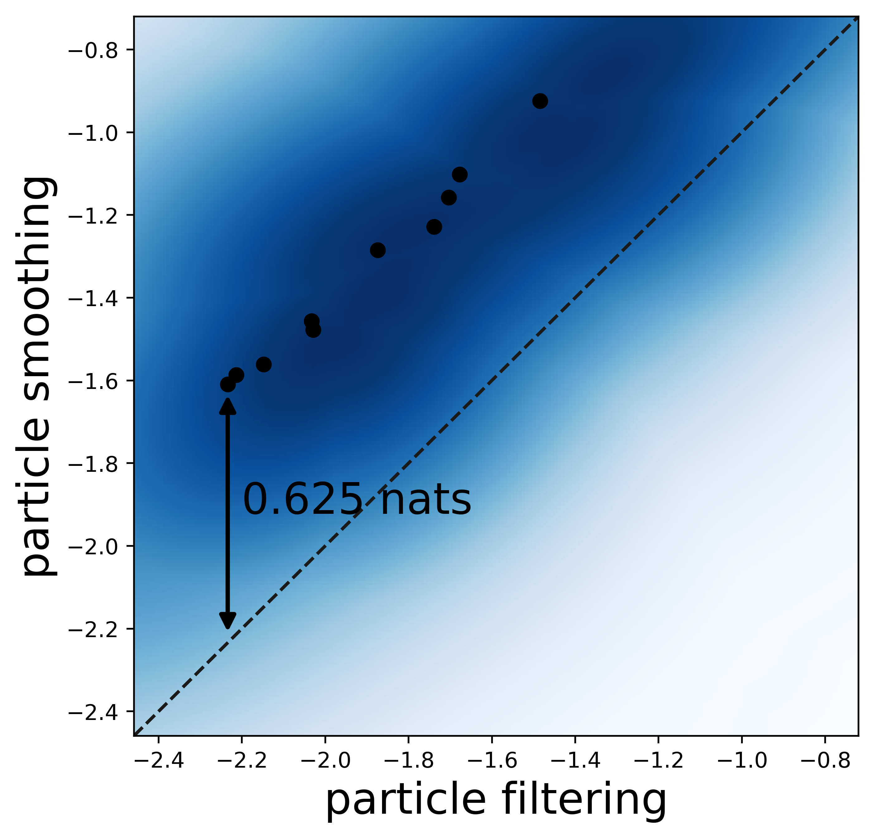
(a) Synthetic Data

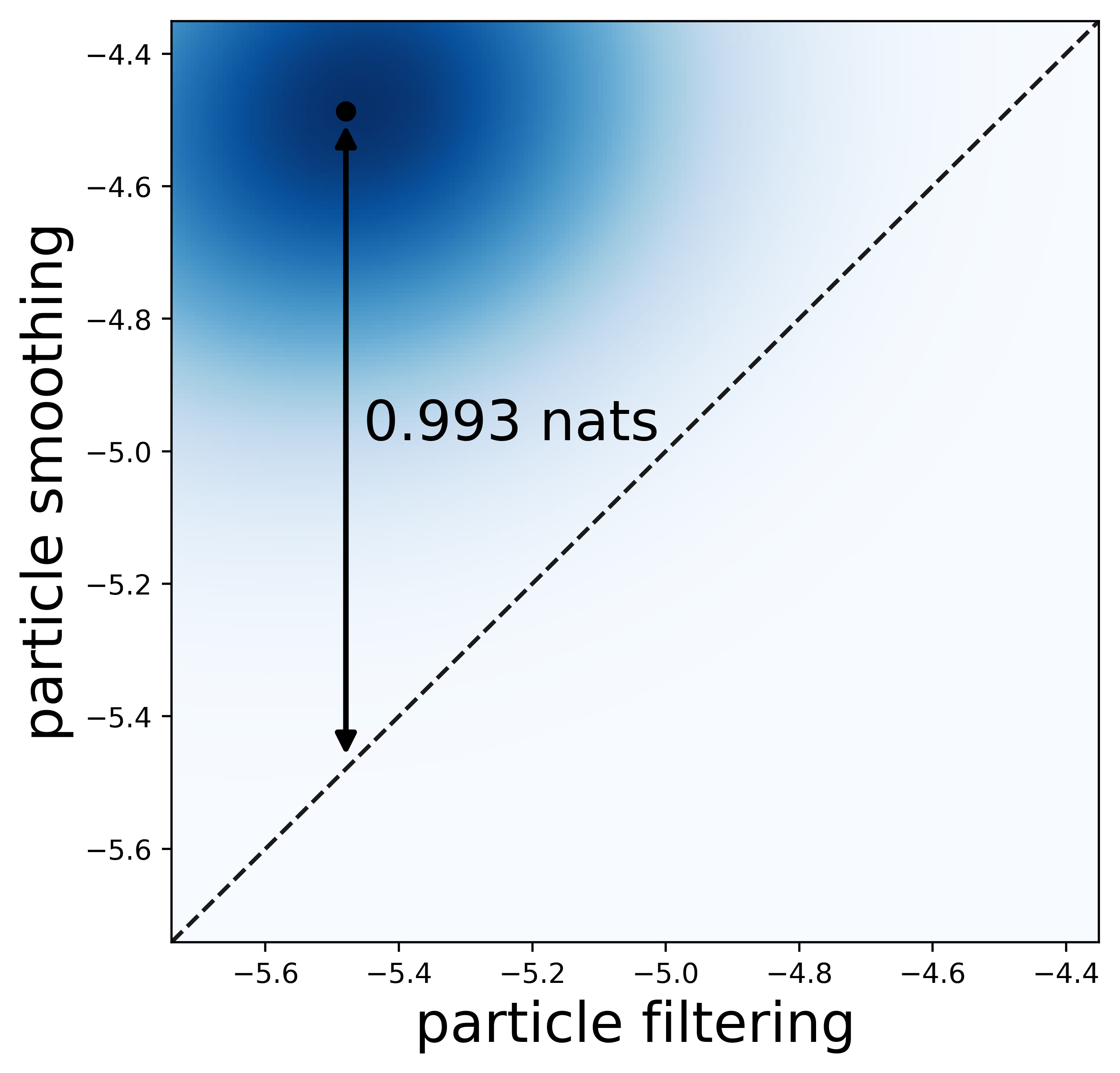
(b) Elevator System

(c) NYC Taxi

Figure 2: Scatterplots of neural Hawkes particle smoothing (y-axis) vs. particle filtering (x-axis) with a stochastic missingness mechanism ($\rho=0.5$). Each point represents a single test sequence, and compares the values of $\log q({{\bm{\mathbf{z}}}^{*}}\mid{\bm{\mathbf{x}}})\;/\;|{{\bm{\mathbf{z}}}^{*}}|$. Larger values mean that the proposal distribution is better at proposing the ground truth ${{\bm{\mathbf{z}}}^{*}}$. Each dataset’s scatterplot is converted to a cloud using kernel density estimation, with the centroid denoted by a black dot. A double-arrowed line indicates the improvement of particle smoothing over filtering. For the synthetic datasets, we draw ten clouds on the same figure and show the line for the dataset where smoothing improves the most. As we can see, the density is always well concentrated above $y=x$. That is, this is not merely an average improvement: nearly every ground truth ${{\bm{\mathbf{z}}}^{*}}$ gets higher proposal probability! Particle smoothing performs well even on datasets where particle filtering performs badly.

5.4 Decoding Results

For each ${\bm{\mathbf{x}}}$, we now make a prediction by sampling an ensemble of $M=50$ particles (section 3) and constructing their consensus sequence $\hat{{\bm{\mathbf{z}}}}$ (section 4.2). We use multinomial resampling since otherwise the effective sample size is very low (only 1–2 on some datasets). We evaluate $\hat{{\bm{\mathbf{z}}}}$ by its optimal transport distance (section 4.1) to the ground truth ${{\bm{\mathbf{z}}}^{*}}$. Note that $\forall{\bm{\mathbf{a}}}$, we can decompose $D(\hat{{\bm{\mathbf{z}}}},{{\bm{\mathbf{z}}}^{*}},{\bm{\mathbf{a}}})$ as

$$C\cdot(\underbrace{|\hat{{\bm{\mathbf{z}}}}|+|{{\bm{\mathbf{z}}}^{*}}|-2|{\bm{\mathbf{a}}}|}_{\text{total insertions+deletions}})+\underbrace{\textstyle{\sum_{(t,t^{*})\in{\bm{\mathbf{a}}}}|t-t^{*}|}}_{\text{total distance moved}}$$ (13)

Letting ${\bm{\mathbf{a}}}$ be the alignment that minimizes $D(\hat{{\bm{\mathbf{z}}}},{{\bm{\mathbf{z}}}^{*}},{\bm{\mathbf{a}}})$, the former term measures how well $\hat{{\bm{\mathbf{z}}}}$ predicts which events happened, and the latter measures how well $\hat{{\bm{\mathbf{z}}}}$ predicts when those events happened. Different choices of $C$ yield different $\hat{{\bm{\mathbf{z}}}}$ with different trade-offs between these two terms. Intuitively, when $C\approx 0$, the decoder is free to insert and delete event tokens; as $C$ increases, $\hat{{\bm{\mathbf{z}}}}$ will tend to insert/delete fewer event tokens and move more of them.

Figure 3 plots the performance of particle smoothing ( ) vs. particle filtering ( ) for the stochastic missingness mechanisms, showing the two terms above as the $x$ and $y$ coordinates. The very similar plots for the deterministic missingness mechanisms are in LABEL:sec:extra-exp (LABEL:fig:eval).

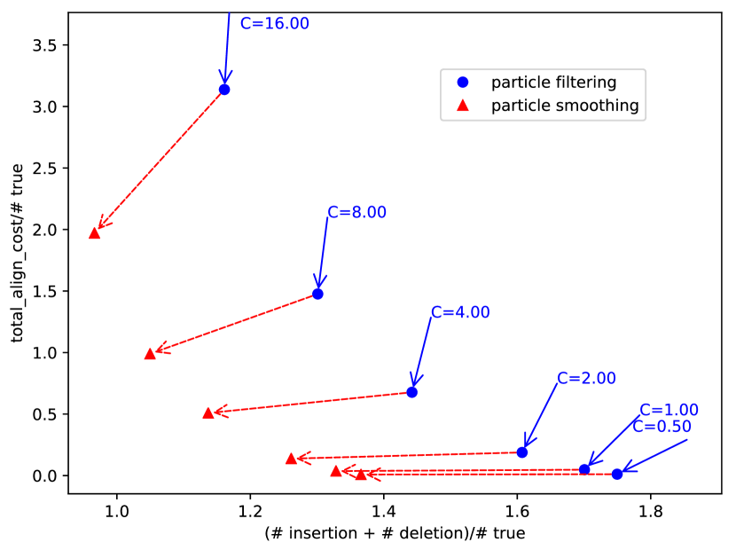
(a) Elevator System

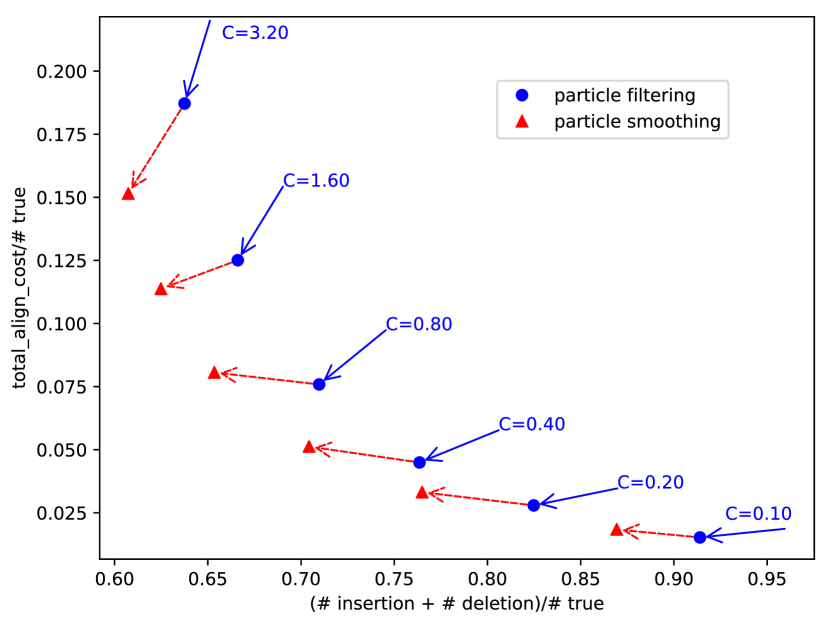
(b) NYC Taxi

Figure 3: Optimal transport distance of particle smoothing ( ) vs. particle filtering ( ) on test data with a stochastic missingness mechanism ($\rho=0.5$). In each figure, the $x$-axis is the total number of deletions and insertions in the test dataset, $\sum_{n=1}^{N}(|\hat{{\bm{\mathbf{z}}}}_{n}|+|{{\bm{\mathbf{z}}}^{*}}_{n}|-2|{\bm{\mathbf{a}}}_{n}|)$, and the $y$-axis is the total movement cost, $\sum_{n=1}^{N}\sum_{(t,t^{*})\in{\bm{\mathbf{a}}}_{n}}|t-t^{*}|$. Both axes are normalized by the true total number of missing events $\sum_{n=1}^{N}|{{\bm{\mathbf{z}}}^{*}}_{n}|$, so the $x$-axis shows a fraction and the $y$-axis shows an average time difference. On each dataset, we show one per $C$. According to equation 13, $(C,1)$, denoted by , turns out to be the gradient of $\sum_{n=1}^{N}D(\hat{{\bm{\mathbf{z}}}}_{n},{{\bm{\mathbf{z}}}^{*}}_{n},{\bm{\mathbf{a}}}_{n})$ at this . The shows the actual improvement obtained by switching to particle smoothing (which is, indeed, an improvement because it has positive dot product with the gradient ). The Pareto frontier (convex hull) of the symbols dominates the Pareto frontier of the symbols—lying everywhere to its left—which means that our particle smoothing method outperforms the filtering baseline.

5.5 Sensitivity to Missingness Mechanism

For the stochastic missingness mechanisms, we also did experiments with different values of missing rate $\rho=0.1,0.3,0.7,0.9$. Our particle smoothing method consistently outperforms the filtering baseline in all the experiments (LABEL:fig:diff_rhos in LABEL:sec:sensitivity_details), similar to Figure 3.

5.6 Runtime

The theoretical runtime complexity is $O(MI)$ where $M$ is the number of particles and $I$ is the number of observed events. In practice, we generate the particles in parallel, leading to acceptable speeds of 300-400 milliseconds per event for the final method. More details about the wall-clock runtime can be found in LABEL:sec:wallclock.

6 Discussion and Related Work

To our knowledge, this is the first time a bidirectional recurrent neural network has been extended to predict events in continuous time. Bidirectional architectures have proven effective at predicting linguistic words and their properties given their left and right contexts (Graves et al., 2013; Bahdanau et al., 2015; Peters et al., 2018; Devlin et al., 2018): in particular, Lin & Eisner (2018) recently applied them to particle smoothing for discrete-time sequence tagging.

Previous work that infers unobserved events in continuous time exploits special properties of simpler models, including Markov jump processes (Rao & Teh, 2012, 2013), continuous-time Bayesian networks (Fan et al., 2010) and Hawkes processes (Shelton et al., 2018). Such properties no longer hold for our more expressive neural model, necessitating our approximate inference method.

Metropolis-Hastings would be an alternative to our particle smoothing method. The transition kernel could propose a single-event change to ${\bm{\mathbf{z}}}$ (insert, delete, or move). Unfortunately, this would be quite slow for a neural model like ours, because any proposed change early in the sequence would affect the LSTM state and hence the probability of all subsequent events. Thus, a single move takes $O(|{\bm{\mathbf{x}}}\sqcup{\bm{\mathbf{z}}}|)$ time to evaluate. Furthermore, the Markov chain may mix slowly because a move that changes only one event may often lead to an incoherent sequence that will be rejected. The point of our particle smoothing is essentially to avoid such rejection by proposing a coherent sequence of events, left to right but considering future ${\bm{\mathbf{x}}}$ events, from an approximation $q({\bm{\mathbf{z}}}\mid{\bm{\mathbf{x}}})$ to the true posterior. (One might build a better Metropolis-Hastings algorithm by designing a transition kernel that makes use of our current proposal distribution, e.g., via particle Gibbs (Chopin & Singh, 2015).)

We also introduced an optimal transport distance between event sequences, which is a valid metric. It essentially regards each event sequence as a 0-1 function over times, and applies a variant of Wasserstein distance (Villani, 2008) or Earth Mover’s distance (Kantorovitch, 1958; Levina & Bickel, 2001). Such variants are under active investigation (Benamou, 2003; Chizat et al., 2015; Frogner et al., 2015; Chizat et al., 2018). Our version allows event insertion and deletion during alignment, where these operations can only apply to an entire event—we cannot align half of an event and delete the other half. Due to these constraints, dynamic programming rather than a linear programming relaxation is needed to find the optimal transport. Xiao et al. (2017) also proposed an optimal transport distance between event sequences that allows event insertion and deletion; however, their insertion and deletion costs turn out to depend on the timing of the events in (we feel) a peculiar way.

We also gave a method to find a single “consensus” reconstruction with small average distance to our particles. This problem is related to Steiner string (Gusfield, 1997), which is usually reduced to multiple sequence alignment (MSA) (Mount, 2004) and heuristically solved by progressive alignment construction using a guide tree (Feng & Doolittle, 1987; Larkin et al., 2007; Notredame et al., 2000) and iterative realignment of the initial sequences with addition of new sequences to the growing MSA (Hirosawa et al., 1995; Gotoh, 1996). These methods might also be tried in our setting. For us, however, the $i$^th event of type $k$ is not simply a character in a finite alphabet such as $\{\texttt{A,C,G,T}\}$ but a time that falls in the infinite set $[0,T)$. The substitution cost between two events of type $k$ is then their time difference.

On multiple synthetic and real-world datasets, our method turns out to be effective at inferring the ground truth sequence of unobserved events. The improvement of particle smoothing upon particle filtering is substantial and consistent, showing the benefit of training a proposal distribution.

Appendix A Little & Rubin (1987)’s Missing-Data Taxonomy

Little & Rubin (1987)’s classical taxonomy of MNAR, MAR, and MCAR mechanisms was meant for graphical models. A graphical model has a fixed set of random variables. The missingness mechanisms envisioned by Little & Rubin (1987) simply decide which of those variables are suppressed in a joint observation. For them, an observed sample always reveals which variables were observed, and thus it reveals how many variables are missing.

In contrast, our incomplete event stream is most simply described as a single random variable $\mathit{Y}$ that is partly missing. If we tried to describe it using $|{\bm{\mathbf{x}}}\sqcup{\bm{\mathbf{z}}}|$ random variables with values like $k{\scriptstyle@}t$, then the observed sample ${\bm{\mathbf{x}}}$ would not reveal the number of missing variables $|{\bm{\mathbf{z}}}|$ nor the total number of variables $|{\bm{\mathbf{x}}}\sqcup{\bm{\mathbf{z}}}|$. There would not be a fixed set of random variables.

To formulate our model in Little & Rubin’s terms, we would need a fixed set of uncountably many random variables $K_{t}$ where $t$ ranges over the set of times. $K_{t}=k$ if there is an event of type $k$ at time $t$, and otherwise $K_{t}=0$. For some finite set of times $t$, we observe a specific value $K_{t}>0$, corresponding to some observed event. For all other times $t$, the value of $K_{t}$ is missing, meaning that we do not know whether or not there is any event at time $t$, let alone the type of such an event. A crucial point is that 0 values are never observed in our setting, because we are never told that an event did not happen at time $t$. In contrast, a value $>0$ (corresponding to an event) may be either observed or unobserved. Thus, the probability that $K_{t}$ is missing depends on whether $K_{t}>0$, meaning that this setting is MNAR.

We preferred to present our model (section 2.1) in terms of the finite sequences that are generated or read by our LSTMs. This simplified the notation later in the paper. But it does not cure the MNAR property: see section 5.1.

Again, our presentation does not allow a Little & Rubin (1987) style formulation in terms of a finite fixed set of random variables, some of which have missing values. That formulation would work if we knew the total number of events $I$, and were simply missing the value $k_{i}$ and/or $t_{i}$ for some indices $i$. But in our setting, the number of events is itself missing: after each observed event $i$, we are missing $J_{i}$ events where $J_{i}$ is itself unknown. In other words, we need to impute even the number of variables in the complete sequence ${\bm{\mathbf{x}}}\sqcup{\bm{\mathbf{z}}}$, not just their values.

Our definition of MAR in section 2.1 is the correct generalization of Little & Rubin (1987)’s definition: namely, it is the case in which the second factor of equation 1 can be ignored. The ability to ignore that factor is precisely why anyone cares about the MAR case. This was mentioned at equation 1, and is discussed in conjunction with the EM algorithm in LABEL:sec:mcem.

Since missing-event settings tend to violate this desirable MAR property, all our experiments address MNAR problems. As Little & Rubin (1987) explained, the more general case of MNAR data cannot be treated without additional knowledge. The difficulty is that identifying $p_{\text{model}}$ jointly with $p_{\text{miss}}$ becomes impossible. If you observe few 50-year-olds on your survey, you cannot know (beyond your prior) whether that’s because there are few 50-year-olds, or because 50-year-olds are very likely to omit their age.

Fortunately, we do have additional knowledge in our setting. Joint identification of $p_{\text{model}}$ and $p_{\text{miss}}$ is unnecessary if either (1) one has separate knowledge of the missingness distribution $p_{\text{miss}}$, or (2) one has separate knowledge of the complete-data distribution $p_{\text{model}}$. In fact, both (1) and (2) hold in the MNAR experiments of this paper (sections 5.1–5.2). But in general, if we know at least one of the distributions, then we can still infer the other (LABEL:sec:mcem).

A.1 Obtaining Complete Data

Readers might wonder why (2) above would hold in a missing-data situation. In practice, where would we obtain a dataset of complete event streams (as in section 5.2) for supervised training of $p_{\text{model}}({\bm{\mathbf{x}}}\sqcup{\bm{\mathbf{z}}})$?

In some event stream scenarios, a training dataset of complete event streams can be collected at extra expense. This is the hope in the medical and user-interface scenarios in section 1. For our imputation method to work on partially observed streams ${\bm{\mathbf{x}}}\sqcup{\bm{\mathbf{z}}}$, their complete streams should be distributed like the ones in the training dataset.

Other scenarios could be described as having eventually complete streams. Complete information about each event stream eventually arrives, at no extra expense, and that event stream can then be used for training. For example, in the competitive game scenario in section 1), perhaps including wars and political campaigns, each game’s true complete history is revealed after the game is over and the need for secrecy has passed. While a game is underway, however, some events are still missing, and imputing them is valuable. Both (1) and (2) hold in these settings.

An interesting subclass of eventual completeness arises in monitoring settings such as epidemiology, journalism, and sensor networks. These often have reporting delays, so that one observes each event only some time after it happens. Yet one must make decisions at time $t<T$ based on the events that have been observed so far. This may involve imputing the past and predicting the future. The missingness mechanism for these reporting delays says that more recent events (soon before the current time $t$) are more likely to be missing. The probability that such an event would be missing depends on the specific distribution of delays, which can be learned with supervision once all the data have arrved.

We point out that in all these cases, the “complete” streams ${\bm{\mathbf{x}}}\sqcup{\bm{\mathbf{z}}}$ that are used to train $p_{\text{model}}$ do not actually have to be causally complete. It may be that in the real world, there are additional latent events ${\bm{\mathbf{w}}}$ that cause the events in ${\bm{\mathbf{x}}}\sqcup{\bm{\mathbf{z}}}$ or mediate their interactions. Mei & Eisner (2017, section 6.3) found that the neural Hawkes process was expressive enough in practice to ignore this causal structure and simply use ${\bm{\mathbf{x}}}\sqcup{\bm{\mathbf{z}}}$ streams to directly train a neural Hawkes process model $p_{\text{model}}({\bm{\mathbf{x}}}\sqcup{\bm{\mathbf{z}}})$ of the marginal distribution of ${\bm{\mathbf{x}}}\sqcup{\bm{\mathbf{z}}}$, without explicitly considering ${\bm{\mathbf{w}}}$ in the model or attempting to sum over ${\bm{\mathbf{w}}}$ values. The assumption here is the usual assumption that ${\bm{\mathbf{x}}}\sqcup{\bm{\mathbf{z}}}$ will have the same distribution in training and test data, and thus ${\bm{\mathbf{w}}}$ will be missing in both, with the same missingness mechanism in both. By contrast, ${\bm{\mathbf{z}}}$ is missing only in test data. It is not possible to impute ${\bm{\mathbf{w}}}$ because it was not modeled explicitly, nor observed even in training data. However, it remains possible to impute ${\bm{\mathbf{z}}}$ in test data based on its distribution in training data.

Appendix B Complete Data Model Details

Our complete data model, such as a neural Hawkes process, gives the probability $p_{\text{model}}({\bm{\mathbf{x}}}\sqcup{\bm{\mathbf{z}}})$ that ${\bm{\mathbf{x}}}\sqcup{\bm{\mathbf{z}}}$ will be the complete set of events on a given interval $[0,T)$. this probability can always be written in the factored form

$$\Big{(}\prod_{i=0}^{I}\prod_{j=0}^{J_{i}}p\!\left(k_{i,j}{\scriptstyle@}t_{i,j}\mid\mathcal{H}(t_{i,j})\right)\Big{)}\cdot p({\scriptstyle@}\!\geq\!T\mid\mathcal{H}(T))$$ (14)

where $p(k{\scriptstyle@}t\mid\mathcal{H}(t))$ denotes the probability density that the first event following $\mathcal{H}(t)$ (which is the set of events occurring strictly before $t$) will be $k{\scriptstyle@}t$, and $p({\scriptstyle@}\geq t^{\prime}\mid\mathcal{H}(t))$ denotes the probability that this event will fall at some time $\geq t^{\prime}$.

Thus, the final factor of (14) is the probability that there are no more events on $[0,T)$ following the last event of ${\bm{\mathbf{x}}}\sqcup{\bm{\mathbf{z}}}$. The initial factor $p(k_{0}{\scriptstyle@}t_{0}\mid\mathcal{H}{t_{0}})$ is defined to be 1, since the boundary event $k_{0}{\scriptstyle@}t_{0}$ is given (see section 2.1).

B.1 Neural Hawkes Process Details

In this section we elaborate slightly on section 2.2. Again, $\lambda_{k}(t\mid\mathcal{H}(t))$ is defined by equation 2 in terms of the hidden state of a continuous-time left-to-right LSTM. We spell out the continuous-time LSTM equations here; more details about them may be found in Mei & Eisner (2017).

$${\bm{\mathbf{h}}}(t)={\bm{\mathbf{o}}}_{i}\odot(2\sigma(2{\bm{\mathbf{c}}}(t))-1)\text{ for }t\in(t_{i-1},t_{i}]$$ (15)

where the interval $(t_{i-1},t_{i}]$ has consecutive observations $k_{i-1}{\scriptstyle@}t_{i-1}$ and $k_{i}{\scriptstyle@}t_{i}$ as endpoints. At $t_{i}$, the continuous-time LSTM reads $k_{i}{\scriptstyle@}t_{i}$ and updates the current (decayed) hidden cells ${\bm{\mathbf{c}}}(t)$ to new initial values ${\bm{\mathbf{c}}}_{i+1}$, based on the current (decayed) hidden state ${\bm{\mathbf{h}}}(t_{i})$, as follows: $\displaystyle{\bm{\mathbf{i}}}_{i+1}$ $\displaystyle\leftarrow\sigma\left({\bm{\mathbf{W}}}_{\mathrm{i}}{\bm{\mathbf{k}}}_{i}+{\bm{\mathbf{U}}}_{\mathrm{i}}{\bm{\mathbf{h}}}(t_{i})+{\bm{\mathbf{d}}}_{\mathrm{i}}\right)$ (16a) $\displaystyle{\bm{\mathbf{f}}}_{i+1}$ $\displaystyle\leftarrow\sigma\left({\bm{\mathbf{W}}}_{\mathrm{f}}{\bm{\mathbf{k}}}_{i}+{\bm{\mathbf{U}}}_{\mathrm{f}}{\bm{\mathbf{h}}}(t_{i})+{\bm{\mathbf{d}}}_{\mathrm{f}}\right)$ (16b) $\displaystyle{\bm{\mathbf{z}}}_{i+1}$ $\displaystyle\leftarrow 2\sigma\left({\bm{\mathbf{W}}}_{\mathrm{z}}{\bm{\mathbf{k}}}_{i}+{\bm{\mathbf{U}}}_{\mathrm{z}}{\bm{\mathbf{h}}}(t_{i})+{\bm{\mathbf{d}}}_{\mathrm{z}}\right)-1$ (16c) $\displaystyle{\bm{\mathbf{o}}}_{i+1}$ $\displaystyle\leftarrow\sigma\left({\bm{\mathbf{W}}}_{\mathrm{o}}{\bm{\mathbf{k}}}_{i}+{\bm{\mathbf{U}}}_{\mathrm{o}}{\bm{\mathbf{h}}}(t_{i})+{\bm{\mathbf{d}}}_{\mathrm{o}}\right)$ (16d) $\displaystyle{\bm{\mathbf{c}}}_{i+1}$ $\displaystyle\leftarrow{\bm{\mathbf{f}}}_{i+1}\odot{\bm{\mathbf{c}}}(t_{i})+{\bm{\mathbf{i}}}_{i+1}\odot{\bm{\mathbf{z}}}_{i+1}$ (17a) $\displaystyle\underline{{\bm{\mathbf{c}}}}_{i+1}$ $\displaystyle\leftarrow\underline{{\bm{\mathbf{f}}}}_{i+1}\odot\underline{{\bm{\mathbf{c}}}}_{i}+\underline{{\bm{\mathbf{i}}}}_{i+1}\odot{\bm{\mathbf{z}}}_{i+1}$ (17b) $\displaystyle{\bm{\mathbf{\delta}}}_{i+1}$ $\displaystyle\leftarrow f\left({\bm{\mathbf{W}}}_{\mathrm{d}}{\bm{\mathbf{k}}}_{i}+{\bm{\mathbf{U}}}_{\mathrm{d}}{\bm{\mathbf{h}}}(t_{i})+{\bm{\mathbf{d}}}_{\mathrm{d}}\right)$ (17c)

The vector ${\bm{\mathbf{k}}}_{i}\in\{0,1\}^{K}$ is the $i$^th input: a one-hot encoding of the new event $k_{i}$, with non-zero value only at the entry indexed by $k_{i}$. Then, ${\bm{\mathbf{c}}}(t)$ for $t\in(t_{i-1},t_{i}]$ is given by (18), which continues to control ${\bm{\mathbf{h}}}(t)$ except that $i$ has now increased by 1).

$${\bm{\mathbf{c}}}(t) \mathrel{\stackrel{{\scriptstyle\textnormal{\tiny def}}}{{=}}}\underline{{\bm{\mathbf{c}}}}_{i+1}+\left({\bm{\mathbf{c}}}_{i+1}-\underline{{\bm{\mathbf{c}}}}_{i+1}\right)\exp\left(-{\bm{\mathbf{\delta}}}_{i+1}\left(t-t_{i}\right)\right)$$ (18)

On the interval $(t_{i},t_{i+1}]$, ${\bm{\mathbf{c}}}(t)$ follows an exponential curve that begins at ${\bm{\mathbf{c}}}_{i+1}$ (in the sense that $\lim_{t\rightarrow t_{i}^{+}}{\bm{\mathbf{c}}}(t)={\bm{\mathbf{c}}}_{i+1}$) and decays, as time $t$ increases, toward $\underline{{\bm{\mathbf{c}}}}_{i+1}$ (which it would approach as $t\rightarrow\infty$, if extrapolated).

The intensity $\lambda_{k}(t\mid\mathcal{H}(t))\in\mathbb{R}_{\geq 0}$ may be thought of as the instantaneous rate of events of type $k$ at time $t$. More precisely, as $dt\rightarrow 0^{+}$, the expected number of events of type $k$ occurring in the interval $[t,t+dt)$, divided by $dt$, approaches $\lambda_{k}(t\mid\mathcal{H}(t))$. If no event of any type occurs in this interval (which becomes almost sure as $dt\rightarrow 0^{+}$), one may still occur in the next interval $[t+dt,t+2dt)$, and so on. The intensity functions $\lambda_{k}(t\mid\mathcal{H}(t))$ are continuous on intervals during which no event occurs (note that $\mathcal{H}(t)$ is constant on such intervals). They jointly determine a distribution over the time of the next event after $\mathcal{H}(t)$, as used in every factor of equation 14. As it turns out (Mei & Eisner, 2017), $\log p_{\text{model}}(\mathit{Y}={\bm{\mathbf{x}}}\sqcup{\bm{\mathbf{z}}})$ becomes

$$\sum_{\ell}\log\lambda_{{k_{\ell}}}(t_{\ell}\mid\mathcal{H}(t_{\ell}))-\int_{t=0}^{T}\sum_{k=1}^{K}\lambda_{{k}}(t\mid\mathcal{H}(t))dt$$ (19)

where the first sum ranges over all events $k_{\ell}{\scriptstyle@}t_{\ell}$ in ${\bm{\mathbf{x}}}\sqcup{\bm{\mathbf{z}}}$.

We can therefore train the parameters ${\bm{\mathbf{\theta}}}$ of the $\lambda_{k}$ functions by maximizing log-likelihood on training data. The first term of equation 19 can be differentiated by back-propagation. Mei & Eisner (2017) explain how simple Monte Carlo integration (see also our LABEL:sec:integral) gives an unbiased estimate of the second term of equation 19, and how the random terms in the Monte Carlo estimate can similarly be differentiated to give a stochastic gradient.

Appendix C Sequential Monte Carlo Details

Our main algorithm is presented as Algorithm 1. It covers both particle filtering and particle smoothing, with optional multinomial resampling.

Algorithm 1 Sequential Monte Carlo — Neural Hawkes Particle Filtering/Smoothing

observed sequence ${\bm{\mathbf{x}}}=k_{0}{\scriptstyle@}t_{0},\ldots,k_{I+1}{\scriptstyle@}t_{I+1}$with $t_{0}=0,t_{I+1}=T$;
model $p$; missingness mechanism $p_{\text{miss}}$; proposal distribution $q$; number of particles $M$;
boolean flags $\mathit{smooth}$and $\mathit{resample}$collection $\{({\bm{\mathbf{z}}}_{1},w_{1}),\ldots,({\bm{\mathbf{z}}}_{M},w_{M})\}$of weighted particles SequentialMonteCarlo${\bm{\mathbf{x}}},p,p_{\text{miss}},q,M,\mathit{smooth},\mathit{resample}$$m=1$to$M$init weighted particles $({\bm{\mathbf{z}}}_{m},w_{m})$. History $\mathcal{H}_{m}$combines ${\bm{\mathbf{z}}}_{m}$with a prefix of ${\bm{\mathbf{x}}}$${\bm{\mathbf{z}}}_{m}\leftarrow\text{empty sequence}$; $w_{m}\leftarrow 1$

References

- Bahdanau et al. (2015) Bahdanau, D., Cho, K., and Bengio, Y. Neural machine translation by jointly learning to align and translate. In Proceedings of the International Conference on Learning Representations (ICLR), 2015.
- Bao et al. (1994) Bao, G., Cassandras, C. G., Djaferis, T. E., Gandhi, A. D., and Looze, D. P. Elevators dispatchers for down-peak traffic, 1994.
- Benamou (2003) Benamou, J.-D. Numerical resolution of an “unbalanced” mass transport problem. ESAIM: Mathematical Modelling and Numerical Analysis, 2003.
- Chizat et al. (2015) Chizat, L., Peyré, G., Schmitzer, B., and Vialard, F.-X. Unbalanced optimal transport: Geometry and Kantorovich formulation. arXiv preprint arXiv:1508.05216, 2015.
- Chizat et al. (2018) Chizat, L., Peyré, G., Schmitzer, B., and Vialard, F.-X. An interpolating distance between optimal transport and Fisher-Rao metrics. Foundations of Computational Mathematics, 2018.
- Chopin & Singh (2015) Chopin, N. and Singh, S. S. On particle Gibbs sampling. Bernoulli, 2015.
- Crites & Barto (1996) Crites, R. H. and Barto, A. G. Improving elevator performance using reinforcement learning. In Advances in Neural Information Processing Systems, 1996.
- Dempster et al. (1977) Dempster, A. P., Laird, N. M., and Rubin, D. B. Maximum likelihood from incomplete data via the EM algorithm. Journal of the Royal Statistical Society. Series B (Methodological), 1977.
- Devlin et al. (2018) Devlin, J., Chang, M.-W., Lee, K., and Toutanova, K. BERT: Pre-training of deep bidirectional transformers for language understanding. arXiv preprint arXiv:1810.04805, 2018.
- Doucet & Johansen (2009) Doucet, A. and Johansen, A. M. A tutorial on particle filtering and smoothing: Fifteen years later. Handbook of Nonlinear Filtering, 2009.
- Doucet et al. (2000) Doucet, A., Godsill, S., and Andrieu, C. On sequential Monte Carlo sampling methods for Bayesian filtering. Statistics and Computing, 2000.
- Du et al. (2016) Du, N., Dai, H., Trivedi, R., Upadhyay, U., Gomez-Rodriguez, M., and Song, L. Recurrent marked temporal point processes: Embedding event history to vector. In Proceedings of the 22nd ACM SIGKDD International Conference on Knowledge Discovery and Data Mining, 2016.
- Fan et al. (2010) Fan, Y., Xu, J., and Shelton, C. R. Importance sampling for continuous-time Bayesian networks. Journal of Machine Learning Research, 2010.
- Feng & Doolittle (1987) Feng, D.-F. and Doolittle, R. F. Progressive sequence alignment as a prerequisite to correct phylogenetic trees. Journal of Molecular Evolution, 1987.
- Frogner et al. (2015) Frogner, C., Zhang, C., Mobahi, H., Araya, M., and Poggio, T. A. Learning with a Wasserstein loss. In Advances in Neural Information Processing Systems, 2015.
- Gotoh (1996) Gotoh, O. Significant improvement in accuracy of multiple protein sequence alignments by iterative refinement as assessed by reference to structural alignments. Journal of Molecular Biology, 1996.
- Graves et al. (2013) Graves, A., Jaitly, N., and Mohamed, A.-R. Hybrid speech recognition with deep bidirectional LSTM. In IEEE Workshop on Automatic Speech Recognition and Understanding (ASRU), 2013.
- Gusfield (1997) Gusfield, D. Algorithms on Strings, Trees and Sequences: Computer Science and Computational Biology. 1997.
- Hawkes (1971) Hawkes, A. G. Spectra of some self-exciting and mutually exciting point processes. Biometrika, 1971.
- Hirosawa et al. (1995) Hirosawa, M., Totoki, Y., Hoshida, M., and Ishikawa, M. Comprehensive study on iterative algorithms of multiple sequence alignment. Bioinformatics, 1995.
- Hochreiter & Schmidhuber (1997) Hochreiter, S. and Schmidhuber, J. Long short-term memory. Neural Computation, 1997.
- Huang et al. (2015) Huang, Z., Xu, W., and Yu, K. Bidirectional LSTM-CRF models for sequence tagging. arXiv preprint arXiv:1508.01991, 2015.
- Kalman (1960) Kalman, R. E. A new approach to linear filtering and prediction problems. Journal of Basic Engineering, 1960.
- Kalman & Bucy (1961) Kalman, R. E. and Bucy, R. S. New results in linear filtering and prediction theory. Journal of Basic Engineering, 1961.
- Kantorovitch (1958) Kantorovitch, L. On the translocation of masses. Management Science, 1958.
- Kingma & Ba (2015) Kingma, D. and Ba, J. Adam: A method for stochastic optimization. In Proceedings of the International Conference on Learning Representations (ICLR), 2015.
- Larkin et al. (2007) Larkin, M. A., Blackshields, G., Brown, N. P., Chenna, R., McGettigan, P. A., McWilliam, H., Valentin, F., Wallace, I. M., Wilm, A., Lopez, R., et al. Clustal W and Clustal X version 2.0. Bioinformatics, 2007.
- Levenshtein (1965) Levenshtein, V. I. Binary codes capable of correcting deletions, insertions, and reversals. In Doklady Akademii Nauk, 1965.
- Levina & Bickel (2001) Levina, E. and Bickel, P. The Earth Mover’s distance is the Mallows distance: Some insights from statistics. In Proceedings of the Eighth IEEE International Conference on Computer Vision (ICCV), 2001.
- Lewis (1991) Lewis, J. A Dynamic Load Balancing Approach to the Control of Multiserver Polling Systems with Applications to Elevator System Dispatching. PhD thesis, University of Massachusetts, Amherst, 1991.
- Lewis & Shedler (1979) Lewis, P. A. and Shedler, G. S. Simulation of nonhomogeneous Poisson processes by thinning. Naval Research Logistics Quarterly, 1979.
- Lin & Eisner (2018) Lin, C.-C. and Eisner, J. Neural particle smoothing for sampling from conditional sequence models. In Proceedings of the 2018 Conference of the North American Chapter of the Association for Computational Linguistics: Human Language Technologies (NAACL-HLT), 2018.
- Linderman et al. (2017) Linderman, S. W., Wang, Y., and Blei, D. M. Bayesian inference for latent Hawkes processes. In Advances in Approximate Bayesian Inference Workshop, 31st Conference on Neural Information Processing Systems, 2017.
- Liniger (2009) Liniger, T. J. Multivariate Hawkes processes. Diss., Eidgenössische Technische Hochschule ETH Zürich, Nr. 18403, 2009.
- Listgarten et al. (2005) Listgarten, J., Neal, R. M., Roweis, S. T., and Emili, A. Multiple alignment of continuous time series. In Advances in Neural Information Processing Systems (NIPS), 2005.
- Little & Rubin (1987) Little, R. J. A. and Rubin, D. B. Statistical Analysis with Missing Data. 1987.
- Liu & Chen (1998) Liu, J. S. and Chen, R. Sequential Monte Carlo methods for dynamic systems. Journal of the American Statistical Association, 1998.
- McLachlan & Krishnan (2007) McLachlan, G. and Krishnan, T. The EM algorithm and Extensions. 2007.
- Mei & Eisner (2017) Mei, H. and Eisner, J. The neural Hawkes process: A neurally self-modulating multivariate point process. In Advances in Neural Information Processing Systems (NIPS), 2017.
- Mohan & Pearl (2018) Mohan, K. and Pearl, J. Graphical models for processing missing data. arXiv preprint arXiv:1801.03583, 2018.
- Moral (1997) Moral, P. D. Nonlinear filtering: Interacting particle resolution. Comptes Rendus de l’Academie des Sciences-Serie I-Mathematique, 1997.
- Mount (2004) Mount, D. W. Bioinformatics: Sequence and Genome Analysis. 2004.
- Notredame et al. (2000) Notredame, C., Higgins, D. G., and Heringa, J. T-Coffee: A novel method for fast and accurate multiple sequence alignment. Journal of molecular biology, 2000.
- Peters et al. (2018) Peters, M., Neumann, M., Iyyer, M., Gardner, M., Clark, C., Lee, K., and Zettlemoyer, L. Deep contextualized word representations. In Proceedings of the 2018 Conference of the North American Chapter of the Association for Computational Linguistics: Human Language Technologies, Volume 1 (Long Papers), 2018.
- Rabiner (1989) Rabiner, L. R. A tutorial on hidden Markov models and selected applications in speech recognition. In Proceedings of the IEEE, 1989.
- Rao & Teh (2012) Rao, V. and Teh, Y. W. MCMC for continuous-time discrete-state systems. In Advances in Neural Information Processing Systems, 2012.
- Rao & Teh (2013) Rao, V. and Teh, Y. W. Fast MCMC sampling for Markov jump processes and extensions. The Journal of Machine Learning Research, 2013.
- Rauch et al. (1965) Rauch, H. E., Striebel, C. T., and Tung, F. Maximum likelihood estimates of linear dynamic systems. AIAA Journal, 1965.
- Sakoe & Chiba (1971) Sakoe, H. and Chiba, S. A dynamic programming approach to continuous speech recognition. In Proceedings of the Seventh International Congress on Acoustics, Budapest, 1971.
- Shelton et al. (2018) Shelton, C. R., Qin, Z., and Shetty, C. Hawkes process inference with missing data. In Proceedings of the AAAI Conference on Artificial Intelligence, 2018.
- Spall (2005) Spall, J. C. Introduction to Stochastic Search and Optimization: Estimation, Simulation, and Control. 2005.
- Villani (2008) Villani, C. Optimal Transport: Old and New. 2008.
- Wei & Tanner (1990) Wei, G. C. G. and Tanner, M. A. A Monte Carlo implementation of the EM algorithm and the poor man’s data augmentation algorithms. Journal of the American Statistical Association, 1990.
- Whong (2014) Whong, C. FOILing NYC’s taxi trip data, 2014.
- Williams (1992) Williams, R. Simple statistical gradient-following algorithms for connectionist reinforcement learning. Machine Learning, 1992.
- Xiao et al. (2017) Xiao, S., Farajtabar, M., Ye, X., Yan, J., Yang, X., Song, L., and Zha, H. Wasserstein learning of deep generative point process models. In Advances in Neural Information Processing Systems (NIPS), 2017.