Parallel and Memory-limited Algorithms for Optimal Task Scheduling Using a Duplicate-Free State-Space

Abstract

The problem of task scheduling with communication delays is strongly NP-hard. State-space search algorithms such as A* have been shown to be a promising approach to solving small to medium sized instances optimally. A recently proposed state-space model for task scheduling, known as Allocation-Ordering (AO), allows state-space search methods to be applied without the need for previously necessary duplicate avoidance mechanisms, and resulted in significantly improved A* performance. The property of a duplicate-free state space also holds particular promise for memory limited search algorithms, such as depth-first branch-and-bound (DFBnB), and parallel search algorithms. This paper investigates and proposes such algorithms for the AO model and, for comparison, the older Exhaustive List Scheduling (ELS) state-space model. Our extensive evaluation shows that AO gives a clear advantage to DFBnB and allows greater scalability for parallel search algorithms.

Department of Electrical and Computer Engineering, University of Auckland, New Zealand

1 Introduction

Efficient schedules are crucial to allowing parallel systems to reach their maximum potential. This work addresses the classic problem of task scheduling with communication delays, known as $P|prec,c_{ij}|C_{\mathrm{max}}$ using the $\alpha|\beta|\gamma$ notation [1]. This problem models a program as a directed acyclic graph of tasks, giving precedence constraints and communication delays, which must be arranged onto a set of processors in order to produce a schedule of minimum length. Solving this problem optimally is NP-hard [2], hence this problem is usually handled with heuristic algorithms, of which a large number have been developed. [3, 4, 5, 6, 7]. The quality of these solutions relative to the optimal cannot be guaranteed, however. [8].

The complexity of the problem usually discourages attempts at optimal solving, but possession of an optimal schedule can make an important difference for time-critical applications. Without optimal solutions, it is also very difficult to evaluate the quality of approximation methods. Branch-and-bound algorithms such as A* have shown some promise in finding optimal schedules, with two notable state-space models having been proposed: exhaustive list scheduling (ELS) [9], and allocation-ordering (AO) [10]. AO, the more recent model, has the advantageous property of being duplicate-free. Under the ELS model, an A* search stores a set of all states encountered so far, and needs to compare every newly reached state with this set in order to mitigate the effect of duplicate states. The duplicate-free property suggests that AO should be more appropriate for the use of parallel state-search algorithms, as it removes the need for storing previous states and the related need for synchronisation between the processors/threads which this entails. It also suggests that AO may give improved performance for search algorithms that do not traditionally have the capacity for duplicate avoidance, such as depth-first branch-and-bound (DFBnB). In this paper, we propose DFBnB of the scheduling problem under AO, and for comparison under ELS. For both A* and DFBnB, we investigate parallelised shared-memory versions and discuss the design decisions. All proposed algorithms are experimentally evaluated with a large set of task graphs of varying properties (e.g. size, structure, computation-to-communication ration, etc.) and different numbers of target processors. We vary the number of threads and employ up to 24 cores in the parallel versions. This paper expands on preliminary work[11], with a more extensive evaluation and additional theoretical discussion throughout.

Section 2 provides background information on the task scheduling problem and the state-space models used, and includes a discussion on related work. Section 3 proposes the DFBnB algorithm for the AO model, while Section 4 investigates the new parallel search algorithms for our scheduling problem. Both Section 3 and Section 4 present the results of the extensive experimental evaluation. Finally, Section 5 presents the conclusions of the paper.

2 Background and Related Work

2.1 Task Scheduling Model

The problem addressed in this work, $P|prec,c_{ij}|C_{\mathrm{max}}$, is the scheduling of a task graph $G=\{V,E,w,c\}$ on a set of processors $P$. $G$ is a directed acyclic graph (or DAG). Each node $n\in V$ is a task belonging to the task graph. Tasks represent an indivisible block of work that must be performed by a program represented by $G$. Each task $n_{i}$ has a weight $w(n_{i})$ which represents the computation time needed to complete that task. An edge $e_{ij}\in E$ represents that task $n_{j}$ relies on task $n_{i}$; data output from $n_{i}$ is required as an input for $n_{j}$, and therefore $n_{j}$ cannot begin execution until $n_{i}$ has finished and communicated the necessary data to $n_{j}$. Each edge $e_{ij}$ has a weight $c(e_{ij})$ which represents the communication time needed to transmit the necessary data from $n_{i}$ to $n_{j}$. Figure 1 shows a simple example of a task graph. The target system for our schedule consists of a finite number of homogeneous dedicated processors, $P$. Each pair of processors $p_{i,}p_{j}\in P$ possess an identical communication link. All communication can be performed concurrently and without contention. Local communication, from $p_{i}$ to $p_{i}$, has no cost.

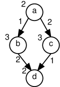
Figure 1: A simple task graph.

We aim to produce a schedule $S=\{proc,t_{s}\}$, where $proc(n)$ gives the processor to which $n$ is assigned, and $t_{s}(n)$ gives the start time of $n$. A valid schedule is one for which all tasks in $G$ are assigned a processor and a start time, and which satisfies two conditions for each task. The first condition, known as the processor constraint, requires that each processor is executing at most one task at any given time. The second condition, known as the precedence constraint, requires that a task $n$ may only begin execution once all of its parents have finished execution, and the necessary data has been communicated to $proc(n)$. Figure 2 shows an example of a valid schedule for the task graph in Figure 1. An optimal schedule is one for which the total execution time is the lowest possible.

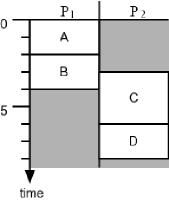
Figure 2: A valid schedule for the simple task graph of Fig. 1.

2.2 Related Work

Many combinatorial optimisation techniques could be used in solving the task scheduling problem. Branch-and-bound search algorithms have been applied to optimal solving of small problem instances, with some success [12, 13]. Previous work using the A* search algorithm has introduced the ELS [9] and AO [10] state-space models, as well as earlier methods [14]. A number of pruning techniques and other optimisations have been developed for ELS [15], producing substantial improvements in performance. Many of these techniques have been adapted for AO as well, and the model has potential for the development of entirely new pruning techniques. Necessary details of these two models will be explained in Section 2.

Integer linear programming (ILP) is an alternative combinatorial optimisation technique which has been applied to this task scheduling problem. Under ILP, problem instances are formulated as a linear program where the variables are constrained to integer values. An optimal solution to the system of equations can then be found, usually with a combination of standard linear programming algorithms and some variety of branch-and-bound search. A variety of ILP formulations for the $P|prec,c_{ij}|C_{\mathrm{max}}$ problem have been proposed [16, 17, 18]. Experiments have shown similarly promising results to those of branch-and-bound, with neither technique showing a significant advantage over the other in terms of the size of task graph that can be practically solved. Popular ILP solvers are mature and highly optimised software packages, but are generally proprietary. This gives them the benefit of a probable speed advantage when compared to a custom implementation of state-space search, but the disadvantage of being somewhat of a “black box”. Using a custom implementation makes it easier to understand the behaviour of the solver, and to gain potentially important insights. It is also often easier to incorporate domain-specific knowledge into a state-space model than into an ILP formulation.

Depth-first branch-and-bound has been applied to various NP-hard problems [19, 20]. As it requires only a small and almost fixed amount of memory, it can allow problem instances to be solved that would be impossible for A* using the memory of a given hardware platform. DFBnB has been previously applied to the ELS model [21]. In this work it was found that, even when using a pruning technique to avoid a portion of duplicate states, significantly fewer problem instances could be solved with DFBnB (or another memory-limited search algorithm, IDA*) than with A* while using the ELS model. The lack of duplicates in the AO model suggests that its use with the DFBnB algorithm will be more successful.

Parallelisation of branch-and-bound has been frequently attempted [22, 23, 24, 25, 26, 27], although no single approach has been found to be dominant over others. Parallel branch-and-bound has not previously been applied to the problem of task scheduling with communication delays.

2.3 Task Scheduling State-Space Models

Branch-and-bound is a family of search algorithms commonly used to solve combinatorial optimisation problems. Through search, they implicitly enumerate all solutions to a problem, and thereby both find an optimal solution and prove that it is optimal [28]. Each node in the search tree, usually referred to as a state, represents a partial solution to the problem. Given a partial solution represented by a state $s$, some operation is applied to produce new partial solutions which are closer to a complete solution. Performing this operation to find the children of $s$ is known as branching. Additionally, every state must be bounded: a cost function $f$ is used to evaluate each state, where $f$ is defined such that $f(s)$ is a lower bound on the cost of any solution that can be reached from $s$. These bounds allow the search to be guided away from unpromising solutions, as a single state can be used to judge the entire subtree that proceeds from it.

One well known variant of branch-and-bound is a best-first search method known as A* [29]. A* has the major advantage that it is optimally efficient; using the same cost function $f$, no search algorithm could find a provably optimal solution while examining fewer states (disregarding states which have the same $f$-value as the optimal). A* relies on the cost function $f$ to always provide an underestimate. This means it is guaranteed that $f(s)\leq f^{*}(s)$, where $f^{*}(s)$ is the true lowest cost of any state in the subtree proceeding from $s$. A function $f$ with this property is said to be admissable. Algorithm 1 gives simple pseudocode for the A*-based scheduling algorithm.

11

Input: $s_{initial}$ is the initial state, an empty allocation

Input: $f(s)$, a lower bound on length of schedules reachable from $s$

Output: An optimal schedule

1 $priorityQueue\leftarrow\emptyset$;

2 Insert $s_{initial}$ into $priorityQueue$ with priority $f(s)$;

3 while $priorityQueue\neq\emptyset$ do

4       $bestState\leftarrow$ pop from $priorityQueue$;

5       if $bestState$ represents a complete schedule then

             // First complete schedule found must be optimal

6             return $bestState$;

      // Solutions that are more complete created by allocating or ordering an additional task

7       for $c\in children(bestState)$ do

8             Insert $c$ into $priorityQueue$ with priority $f(c)$;

9            

10      

Algorithm 1 Pseudocode for the A* algorithm.

2.3.1 Exhaustive List Scheduling State-Space

Exhaustive list scheduling (ELS) is a state-space model for optimal task scheduling which bears a strong resemblance to list scheduling heuristic methods for approximate task scheduling. In this model, each state is a partial schedule. Each task is either scheduled or unscheduled in each state. If a task is scheduled, then it has been assigned to a processor and given a start time. If a task is unscheduled, it may be “free” or not free. A task is free if all of its dependencies have been met; that is, if all of its parents have already been scheduled. At each step, the model branches by placing any free task onto any processor. The full set of children of a state $s$ therefore represent all possible free tasks that could have been chosen, and all possible processors they could have been placed on [9]. In this way, the model simulates all possible decisions that a list scheduling algorithm could make. An example can be seen in Figure 3, demonstrating the four possible child states of a partial schedule with two processors and two free tasks.

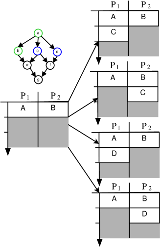
Figure 3: Branching in the ELS state space.

Branch-and-bound methods are most effective when the state-space they are searching has the property that all subtrees are disjoint. This means that there is only one path from the root of the tree to any state in the state-space. When this is not the case, we refer to any paths that lead to a state already visited ’duplicates’. Equivalently, any state reached which has already been encountered is termed a ’duplicate’ state. If duplicate states are not detected, then the search algorithm can perform a substantial amount of unnecessary work: not only might they examine one duplicate state when an alternate path is found, they may also proceed to re-explore the entire subtree rooted at that state. Detecting duplicate states requires keeping a record of those states which have already been visited, which represents a significant investment of memory.

Unfortunately, the ELS strategy creates a lot of potential for duplicated states . One type, which we call processor permutation duplicates, arise when multiple partial schedules can be transformed into each other merely by relabeling their processors. These duplicates can be efficiently avoided in ELS using a processor normalisation pruning technique[15]. Another type which are fundamental to the model are independent decision duplicates. Tasks which are independent of each other can be selected for scheduling in different orders, but be assigned to the same processors in each case. Performing the same scheduling decisions in a different order constitutes taking a different path to reach the same partial schedule, and therefore a duplicate state. Figure 4 shows two possible paths leading to the same state. These duplicates can only be avoided by enforcing a specific sequence onto these scheduling decisions. There is no known method by which this can be achieved under the ELS model, while still allowing all possible schedules to be reached.

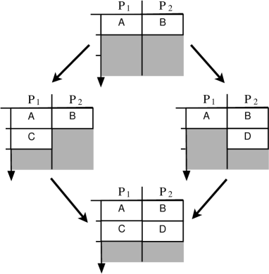
Figure 4: Independent decision duplicates.

2.3.2 Allocation-Ordering State-Space

Allocation-Ordering (AO) is a new state-space model [10] constructed such that a specific order is enforced on all scheduling decisions, and therefore the duplicates found in ELS do not exist. The model is named for the two distinct phases in which it creates a schedule: first Allocation, where each task is assigned to a processor, and then Ordering, where a sequence is decided for the set of tasks allocated to each processor. As it first decides how tasks are grouped together on processors, this model bears a resemblance to the scheduling approximation methods known as clustering [30, 31, 32], whereas ELS resembles list scheduling.

In the Allocation phase, a partition of the set of tasks is built iteratively, with the maximum number of subsets in the partition being the number of processors available for scheduling. At each step, the current task can either be added to one of the existing subsets, or used to begin a new subset. This process allows all possible groupings of the tasks to be reached, with only one possible path to each grouping.

The Ordering phase begins with a complete allocation. From there, it proceeds in a manner similar to ELS, but on a per-processor basis. For a processor $p_{i}$, a task $n_{i}$ allocated to $p_{i}$ is considered to be “free” for ordering if there is no task $n_{j}$ also on $p_{i}$ which is an ancestor of $n_{i}$ in the task graph $G$. At each step, one task is selected from among all those which are currently free on $p_{i}$, and placed next in order. This is repeated until all tasks on $p_{i}$ have been given a place in the sequence. The decision of which processor to order a task on next can be made arbitrarily, but it must be deterministic such that the processor which is selected can be determined entirely by the depth of the current state. A simple round-robin method will suffice. Once this process has been completed for all processors, a complete schedule can be derived, simply by giving each task its earliest possible start time given the processor and place in sequence it has been assigned. Figure 5 provides a view of the overall AO state-space , showing how the Allocation phase leads into the Ordering phase and how a search algorithm might move seamlessly back and forth between them.

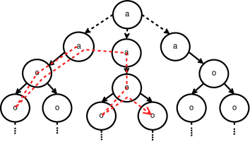
Figure 5: A view of the AO state-space, including both phases.

By assigning each task to a processor first, and enforcing a strict order in which the processors are considered, this model eliminates the possibility of independent decision duplicates. In ELS it was possible to place task $n_{1}$ on $p_{1}$ and then $n_{2}$ on $p_{2}$, but equally valid to place $n_{2}$ on $p_{2}$ before placing $n_{1}$on $p_{1}$. AO can force $p_{1}$ to be considered before $p_{2}$, making only the first sequence of decisions a possibility.

3 Depth-First Branch and Bound

Depth-first branch-and-bound (DFBnB) is a variant of branch-and-bound which uses a depth-first search strategy, moving as far into the state-space as possible before back-tracking to try other paths. Just as with A*, a cost function $f$ is used to evaluate each state $s$, producing a lower bound $f(s)$ on the quality of any solution which could be reached from $s$. When DFBnB first encounters a state $s_{c}$ representing a complete solution, the cost $f(s_{c})$ is recorded as $f_{best}$. Subsequently, if a state is encountered such that $f(s)\geq f_{best}$, the search will not proceed to that state’s children; we have already found a solution at least as good as any that can be reached from this state. If another complete solution $s_{c^{\prime}}$ is encountered, and $f(s_{c^{\prime}})<f_{best}$, then $f_{best}$ is overwritten with $f(s_{c^{\prime}})$. The search ends when no further states can be reached with $f(s)<f_{best}$. At this point, the complete solution with cost $f_{best}$ has been proven to be optimal. Algorithm 2 gives simple pseudocode for the DFBnB algorithm.

The most obvious advantage of DFBnB when compared with A* is its much lower memory requirements. The best-first nature of A* necessitates the maintenance of a priority queue requiring $O(b^{d})$ space (where $d$ refers to the depth of the state-space and $b$ is its average branching factor). A depth-first search requires only states on the current path and their children to be in memory at any given time, using $O(bd)$ space. In the case of task scheduling, this means the memory requirement of A* scales exponentially with the number of tasks, while for DFBnB it scales only linearly. The memory requirement for DFBnB is small and predictable enough that in practical application it can usually be treated as constant. A related advantage is that the data structures used in depth-first search (usually a stack) tend to be much smaller and simpler, and therefore operations performed on them are expected to take less time. This is likely to mean that a depth-first search can process states at a faster rate than a best-first search.

Naturally, DFBnB also has several disadvantages when compared to A*. The first is that, since it is a depth-first search, it cannot be applied to state-spaces of infinite depth without careful modification. As both AO and ELS have a finite (and relatively shallow) depth, this is not important to our application.

Another disadvantage is that, unlike A*, DFBnB is not optimally efficient. Like A*, DFBnB will always examine every state which has $f(s)$ less than the optimal solution, but it is likely that DFBnB will also examine states with $f(s)$ greater than the optimal solution, which A* will never examine. Indeed, the only case in which DFBnB will not examine extraneous states is if the very first complete solution it encounters is also optimal. This does not mean that DFBnB is guaranteed to examine more states in total than A*; if A* happens to examine a greater proportion of those states where $f(s)$ is equal to the optimal solution, it can still end up doing more work. Such situations, however, are strongly implementation-dependent and unpredictable. It is prudent to assume that, for an arbitrary problem instance, DFBnB is likely to perform more work overall.

When applying DFBnB to a state-space containing duplicate states, there are two possible approaches: ignore the duplicates, or implement a duplicate-detection mechanism. If we ignore duplicate states, we are likely to greatly increase the amount of work necessary to find the optimal solution. A depth-first search will examine every possible path in the state-space: this could mean that entire sub-trees are explored many times over. On the other hand, the addition of a duplicate-detection mechanism will largely negate the main advantage of DFBnB over A*, that being its much lower $O(bd)$ memory requirement. In order to avoid repeating work, the search algorithm must keep a record of states it has already examined. Although many strategies could exist for deciding exactly which states should be remembered, any strategy that is maximally effective at detecting duplicates will require $O(b^{d})$ memory, just as A* does. With such an implementation of DFBnB requiring an exponentially growing amount of memory, and not being optimally efficient, it is hard to imagine a situation in which it would be preferable to A*.

For those reasons, it seems likely that DFBnB would perform significantly better on AO, a duplicate-free state-space, than it would on ELS, a state-space with duplicates. If this is true, then the use of AO could make DFBnB a more practical option for optimal task scheduling, making its benefits available for situations where memory is the more constraining factor.

15

Input: $s_{initial}$ is the initial state, an empty allocation

Input: $f(s)$, a lower bound on length of schedules reachable from $s$

Output: An optimal schedule

1 $stack\leftarrow\emptyset$;

2 Push $s_{initial}$ onto $stack$;

3 $bestSolution\leftarrow\infty$;

4 while $stack\neq\emptyset$ do

5       $currentState\leftarrow$ pop from $stack$;

6       if $f(currentState)<f(bestSolution)$ then

             // Solutions that are more complete created by allocating or ordering an additional task

7             for $c\in children(currentState)$ do

8                   Push $c$ onto $stack$;

9                  

10            if $currentState$ represents a complete schedule then

                   // Schedule is best known but not confirmed optimal

11                   $bestSolution\leftarrow currentState$;

12                  

13            

14      

return $bestSolution$;

Algorithm 2 Pseudocode for the DFBnB algorithm.

3.1 Evaluation

To experimentally evaluate the hypothesis that AO would allow better performance from depth-first branch-and-bound, we performed DFBnB searches on a set of task graphs using each state-space model. The evaluation was performed by running branch-and-bound searches on a diverse set of task graphs using each state-space model. Task graphs were chosen that differed by the following attributes: graph structure, the number of tasks, and the communication-to-computation ratio (CCR). Table 1 describes the range of attributes in the data set. A set of 1020 task graphs with unique combinations of these attributes were selected. These graphs were divided into three groups according to the number of tasks they contained: 16 tasks, 21 tasks, or 30 tasks. An optimal schedule was attempted for each task graph using 2, 4, and 8 processors, once each for each state-space model. This made a total of 3060 problem instances attempted per model. Gathering this data took approximately one week of continuous server time.

Graph structure	No. of tasks	CCR values
• Independent • Fork • Join • Fork-Join • Out-Tree • In-Tree • Pipeline • Random • Series-Parallel	• 16 • 21 • 30	• 0.1 • 1 • 10

Table 1: Range of task graphs in the experimental data set.

The algorithms were implemented in the Java programming language. Existing implementations of both ELS and AO were utilised. All tests were run on a Linux machine with 4 Intel Xeon E7-4830 v3 @2.1GHz processors. The tests were single-threaded, so they would only have gained marginal benefit from the multi-core system. The tests were allowed a time limit of 2 minutes to complete. For all tests, the JVM was given a maximum heap size of 96 GB. Each search was started in a new JVM instance, to remove the possibility of previous searches impacting them through garbage collection and JIT compilation.

Figure 6 shows the results of these tests as performance profiles: the $x$-axis shows time elapsed, while the $y$-axis shows the cumulative percentage of problem instances which were successfully solved by this time. In all three groups of task graphs, it is clear that substantially more problem instances were solved with AO than with ELS. In the 16 task group, ELS solved 64% of problem instances while AO solved 96%. This is both a large difference in absolute terms and a relative advantage of 50% for AO. Similarly, in the 30 task group, ELS solved 18% while AO solved 28%. This is a relative advantage of 55% for AO. In the 21 task group ELS solved 43% and AO solved 81%, giving a relative advantage of 88% for AO. These results make it clear that AO is a significantly better choice than ELS when using DFBnB. This performance is comparable to what was previously observed when using AO with the A* algorithm [33], suggesting that in practice DFBnB does not perform significantly worse than A*. Along with the low memory cost, the performance demonstrated here makes a strong case for DFBnB as the primary branch-and-bound method for optimal task scheduling, which is different to previous results when the ELS model is employed [21]. As well as removing the possibility of failure due to memory exhaustion, DFBnB could be used to solve many problem instances simultaneously on a multicore system as there is no competition for memory from which simultaneous A* runs would suffer.

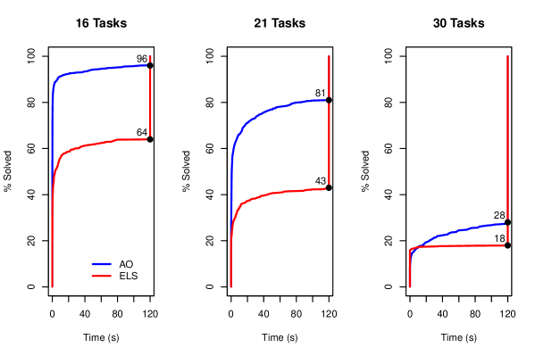
Figure 6: Comparing the performance of DFBnB using AO and ELS.

4 Parallel Search

State-space search is very time consuming, even when using a good state-space model with effective cost functions and pruning techniques. Accelerating a search through parallelisation may be critical to obtaining a solution within an acceptable timeframe. As the AO model is duplicate-free, it does not require the use of a duplicate-detection mechanism, or any of the data structures associated with one. In a parallelised implementation of branch-and-bound, these data structures require synchronisation between workers, adding greatly to the potential for contention and likely limiting overall speedup. Therefore, without the need for duplicate detection, it seems probable that parallel branch-and-bound could be more effective when used with the AO model than with the ELS model. In this section we investigate and propose shared-memory parallel versions of both A* and DFBnB. Branch-and-bound search has several features which make parallelisation a non-trivial task [34]. We describe the different factors that were considered, and discuss the decisions made at each step. Usually, the final decision was based on the results of preliminary experimentation with the identified options. We will describe two parallel algorithms, sharing many characteristics. One, based on DFBnB, we will refer to as PDFS. The other, based on A*, we will refer to as PA*. For comparison purposes there is a variant of PA* which includes a duplicate detection mechanism, which we will refer to as PA*-DD. Algorithm 3 gives pseudocode for PA* and PA*-DD, and Algorithm 4 gives pseudocode for PDFS.

4.1 Work Decomposition

4.1.1 Unit of Work

We start by identifying the parallelisable work in the algorithm. Branch-and-bound search inherently comes with a division of work into discrete and independent jobs (or tasks; in order to avoid confusion, we will use the term job here). The natural unit of work is the expansion of each individual state. Given two states, the children of each can be constructed and evaluated simultaneously without any interaction between processes.

4.1.2 Central

Given this, a natural method of parallelisation is a simple thread pool, with a job queue from which a number of workers take states and expand them, subsequently inserting the produced children back into the queue. This method is visualised in Figure 7. It is usual to implement A* with a priority queue, so this does not require an especially large change to the implementation of the algorithm. However, use of this simple thread pool model is complicated by the way in which A* requires the job queue to be used. The expansion of a state will usually result in the creation of multiple child states, which must then be added to the queue. This means that there must be many more jobs inserted than retrieved, and the queue will inevitably grow quickly. Since the best-first nature of A* necessitates a priority queue, each of these insertions requires a non-trivial amount of work - for a heap-based priority queue with current size $n$, this is $O(log(n))$ time. Unlike a standard queue, insertions may cause changes to any part of the data structure, meaning that parallel insertions and retrievals may conflict with each other. The combination of these factors makes operations on the priority queue a major source of contention between workers. Investigation using Java’s PriorityBlockingQueue data structure, a standard binary heap with a global lock, showed no speedup at all. Although a more complex data structure may have allowed better performance, such as the more granularly locked pipelined priority queue [35] or the lock-free skiplist [36], it is clear that an effective parallelisation using this strategy is not so simple to implement as it may seem. Previous research has also found that such an approach lead to performance worse than sequential A*[26].

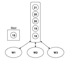
Figure 7: Workers sharing a central priority queue.

4.1.3 Distributed

Instead of considering individual states as the basic unit of work, we can instead have workers process entire sub-trees of the state-space, as shown in Figure 8. Each worker has its own queue of states, which it can retrieve from as needed and to which it will return all child states produced. This is a more coarse-grained parallelisation strategy, requiring much less interaction between workers. It does require, however, that states are initially distributed between the workers. This can be achieved by beginning with a stage in which a serial A* search is run until its queue contains enough states to provide work for all workers. The states can then be assigned to workers in round-robin fashion. Each worker is then free to work on its own sub-tree, performing its own search mostly in isolation. In the case of PA*, a heap-based priority queue is used, while PDFS uses a linked-list-based deque.

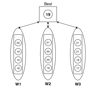
Figure 8: Distributed priority queues.

4.2 Worker Synchronisation

It is still necessary for some regular communication between workers to occur in order for the overall search to be most efficient. The problem with having sub-trees searched in isolation is that, since the workers only have partial information about the state-space, the pure best-first property of A* is no longer maintained. Although each worker may select the best among the options available to it, there is no guarantee that the selected state is anywhere close to the true best currently available in the overall search. This means that A*’s property of optimal efficiency no longer holds, and many of the states expanded by a given worker may never have been touched by a serial A* search. Similarly in a parallel DFBnB search if one worker has already found a good solution but the other workers, without knowledge of this, continue to expand states which could not lead to a better solution, the time spent doing so is wasted. To mitigate this, we must share information between workers, allowing them to more often determine when expanding a particular state would be wasted work. The more frequently information is shared, the closer to optimally efficient we can be, but the greater the synchronisation overhead will become. A simple way to do this, which works for both A* and DFBnB, is to maintain a public record of the best solution found so far in the overall search. Whenever a worker finds a complete solution, it can compare it against this value, and update it if its new solution is better. Workers will only examine states in their assigned sub-trees with a lower $f$-value than their currently best known solution. After examining a number of states (this is a tuneable parameter, and we currently use onehundred thousand) they will check to see if any other worker has discovered a better solution. With depth-first search, solutions are expected to be discovered very often early on, and less so as the optimal is approached. With A*’s best-first approach, the opposite is expected, with no solutions at all found until near the end of the search.

4.2.1 Duplicate Detection

The PA*-DD variant is defined by an additional data structure shared between all the workers for the purposes of duplicate detection. The data structure used is a hashmap: in our implementation, Java’s ConcurrentHashMap, a thread-safe hash map designed for high concurrency. When any worker creates a new state, it will check if an identical state already exists in the hashmap. If it does, the new state is a duplicate and is discarded. If it does not, the new state is added to the hashmap and the algorithm proceeds as normal.

4.3 Load Balancing

Using entire sub-trees as units of work leads to another issue: it is impossible to determine a priori the amount of useful work represented by a given sub-tree. Some root states may represent very bad decisions, such that little or none of their descendants would be considered by a serial A* search. Others may represent especially good decisions, such that almost all states worth examining belong to their sub-tree. This huge potential imbalance in work between sub-trees means that some workers will finish much earlier than others, causing speedup potential to be lost. To aid with load-balancing, we therefore employ work-stealing [37]. When a worker has exhausted all potentially useful work in its own sub-tree, it visits another worker and takes a state from it, as shown in Figure 9. For DFBnB, a state is stolen from the back end of the deque. This both minimises the chance of contention between the thief and the victim, and maximises the total amount of work stolen - since states at the tail of the deque are highest up in the state-space, they lead to the largest subtrees. This will hopefully ensure that the thief does not have to steal again soon after. For A*, it is the current best state in the victim’s priority queue that is taken - meaning that it is the most likely state present to lead to the optimal solution, and therefore most likely to represent useful work. By contrast, stealing from the back of the queue could yield a very low quality state which, if it is useful to examine it at all, is relatively unlikely to lead to a significantly sized worthwhile subtree. Stealing only a single state will minimise the impact of synchronisation on the victimised worker. For both approaches, the victims of stealing are selected randomly, which is the standard method [38]. This tends to spread the burden of victimisation uniformly and requires little communication between threads for a decision to be made.

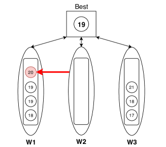
Figure 9: A worker with an empty queue steals from another.

4.4 Termination

Another complication of this parallel branch-and-bound algorithm is the difficulty of determining when a provably optimal solution has been found, and the search can be terminated. In serial A*, the best-first property ensures that the very first complete solution found must necessarily be optimal. In this parallel version, the best-first property is no longer maintained globally. Not only does this mean that complete but non-optimal solutions may be discovered first, but true optimal solutions may not immediately be able to be proven optimal. In order to prove that a solution is optimal, both in A* and in DFBnB, all states of lower $f$-value in the state-space must have been examined and shown not to be complete solutions. Figures 7 and 8 both depict a situation in which a complete solution has been found (and stored as the best known solution) while one or more states remain in the queue(s) which have a lower f-value. For PDFS, this is part of standard operation. If the algorithm being used is PA*, however, this must mean that the loss of the strict best-first property led to one worker discovering this complete solution while another worker was creating a child state with a lower f-value. In both algorithms, a worker without any of these lower-$f$-value states no longer has any useful work in its queue, and it will attempt to steal a promising state from another worker. An individual worker will know that it should terminate when it has no more useful work in its queue, and there are no other workers with work available to steal. The search will be finished only once all workers have exhausted their queues of states with $f$-values lower than the current best known solution.

52

Input: $S_{i}$, a set of states produced by sequential A*

Input: global $W$, a set of workers

Input: global atomic $bestSolution\leftarrow\infty$

Input: global atomic $idleWorkerCount\leftarrow 0$

Output: An optimal schedule

1

2$priorityQueue\leftarrow$ all $s\in S_{i}$, accessible as $W_{i}[PQ]$;

3 $hasWork\leftarrow True$, accessible as $W_{i}[hasWork]$;

4 $localBestKnown\leftarrow bestSolution$;

5 $syncCounter\leftarrow 0$;

6

7if $duplicateDetection=True$ then

8       Insert all $s\in S_{i}$ into $hashmap$;

9      

10while idleWorkerCount < |W| do // at least one worker has work

11       while $priorityQueue\neq\emptyset$ do

12             $bestState\leftarrow$ pop from $priorityQueue$;

13            

14            $syncCounter\leftarrow syncCounter+1$;

15             if $syncCounter=syncThreshold$ then // Periodic sync

16                   $localBestKnown\leftarrow bestSolution$;

17                   $syncCounter\leftarrow 0$;

18                  

19            if $f(bestState)<f(localBestKnown)$ then

20                   if $complete(bestState)$ then

21                         Test-and-set $bestSolution\leftarrow bestState$;

22                        

23                  for $c\in children(bestState)$ do

24                         if $f(c)<f(localBestKnown)$ then

25                               if $duplicateDetection=True$ then // DD variant

26                                     if $c\notin hashmap$ then

27                                           Insert $c$ into $hashmap$;

28                                           Insert $c$ into $priorityQueue$ with priority $f(c)$;

29                                          

30                                    

31                              else

32                                     Insert $c$ into $priorityQueue$ with priority $f(c)$;

33                                    

34                              

35                        

36                  

37            else // No more useful work

38                   $priorityQueue\leftarrow\emptyset$;

39                  

40            

41      $hasWork\leftarrow False$;

42       Test-and-set $idleWorkerCount\leftarrow idleWorkerCount+1$;

43      

44      $victim\leftarrow$ a random number from $0$ to $|W|$;

45       if $W_{victim}[hasWork]=True$ then // Work Stealing

46             $stolenState\leftarrow$ pop head from $W_{victim}[PQ]$;

47             Insert $stolenState$ into $priorityQueue$;

48             $hasWork\leftarrow True$;

49             Test-and-set $idleWorkerCount\leftarrow idleWorkerCount-1$;

50            

51      

return $bestSolution$

Algorithm 3 Pseudocode for a single PA* worker.

39

Input: $S_{i}$, a set of states produced by sequential A*

Input: global $W$, a set of workers

1

Input: global atomic $bestSolution\leftarrow\infty$

Input: global atomic $idleWorkerCount\leftarrow 0$

Output: An optimal schedule

2

3$stack\leftarrow\emptyset$, accessible as $W_{i}[stack]$;

4 $hasWork\leftarrow True$, accessible as $W_{i}[hasWork]$;

5 $localBestKnown\leftarrow bestSolution$;

6 $syncCounter\leftarrow 0$;

7 Push all $s\in S_{i}$ onto $stack$;

8 while idleWorkerCount < |W| do // at least one worker has work

9       while $stack\neq\emptyset$ do

10             $currentState\leftarrow$ pop from $stack$;

11            

12            $syncCounter\leftarrow syncCounter+1$;

13             if $syncCounter=syncThreshold$ then // Periodic sync

14                   $localBestKnown\leftarrow bestSolution$;

15                   $syncCounter\leftarrow 0$;

16                  

17            if $f(currentState)<f(localBestKnown)$ then

18                   if $complete(currentState)$ then

19                         Test-and-set $bestSolution\leftarrow currentState$;

20                        

21                  for $c\in children(bestState)$ do

22                         if $f(c)<f(localBestKnown)$ then

23                               Push $c$ onto $stack$;

24                              

25                        

26                  

27            

28      $hasWork\leftarrow False$;

29       Test-and-set $idleWorkerCount\leftarrow idleWorkerCount+1$;

30      

31      $victim\leftarrow$ a random number from $0$ to $|W|$;

32       if $W_{victim}[hasWork]=True$ then // Work Stealing

33             $stolenState\leftarrow$ pop tail from $W_{victim}[stack]$;

34             Push $stolenState$ onto $stack$;

35             $hasWork\leftarrow True$;

36             Test-and-set $idleWorkerCount\leftarrow idleWorkerCount-1$;

37            

38      

return $bestSolution$

Algorithm 4 Pseudocode for a single PDFS worker.

4.5 Evaluation

To experimentally evaluate the hypothesis that AO would allow better performance for parallel search algorithms, we performed parallel searches on a set of task graphs using the proposed parallel algorithms of A* and DFBnB. Task graphs were chosen that differed by graph structure and communication-to-computation ratio (CCR). From the larger dataset described in Table 1, the group of graphs with 21 tasks were selected. This is a set of 340 task graphs. We attempted to find an optimal schedule with 4 processors, for both state-space models, using 1, 2, 4, 8, 16 and 24 worker threads, once each for PDFS and PA*. For each trial using ELS with PA*, an additional trial using PA*-DD was added. This gave a total of 10,200 trials. The algorithms were implemented in the Java programming language, based on sequential implementations of both ELS and AO [33]. All tests were run on a Linux machine (Ubuntu 16.04) with 4 Intel Xeon E7-4830 v3 @2.1GHz processors. This system has a total of 48 cores. Each trial wasallowed a time limit of 2 minutes to complete. For all tests, the JVM (Java HotSpot 25.91) was given a maximum heap size of 96 GB. Each search was started in a new JVM instance, to remove the possibility of previous searches impacting them through garbage collection and JIT compilation.

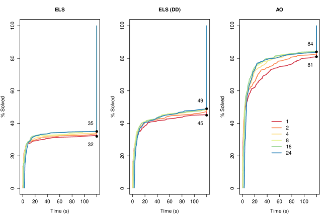
Figure 10: Performance profiles for PA* and PA*-DD

Figure 10 shows performance profiles (as described in Section 3) demonstrating how performance with PA* varied across the range of threads used. It is clear from these profiles that the AO model consistently has the best absolute performance, solving the most instances after any given time, while ELS solves significantly less instances without duplicate detection. This confirms our expectations regarding the state-space models and the importance of duplication detection.

All three variants show some amount of performance increase, scaling with the number of threads. By the time limit of 2 minutes, the multithreaded variants solved 3-4% more instances than in the sequential case. However, with AO, we can see clearly that at earlier times there are greater differences between the curves, suggesting that parallelisation is in fact solving instances much quicker. The flattening of all the curves tells us that fewer and fewer problem instances are solved as time goes on, which is the expected effect in an exponential state-space search.This effect allows the sequential algorithm (and parallelisation with lower number of threads) to “catch up”.

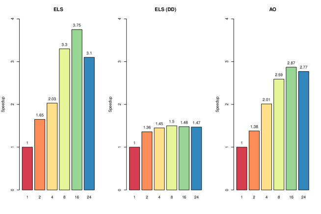
Figure 11: Speedup of PA* at 60 seconds over different number of threads.

In order to better analyse the scaling of the parallel algorithm, and considering the flattening effect just discussed, we calculate the speedup after $x$ seconds of the parallel algorithm with $n$ threads as follows: first, we find the number of problem instances solved by the sequential algorithm within $x$ seconds,$\text{seqnum}(x)$. Then, we find the time taken for the parallel algorithm with $n$ threads to solve $\text{seqnum}(x)$ problem instances, $\text{partime}_{n}(\text{seqnum}(x))$. Finally, the speedup is defined as $\text{speedup}(n,x)=x/(\text{partime}_{n}(\text{seqnum}(x)))$. Figure 11 shows the result of this calculation across our dataset with $x$ at 60 seconds. By this metric we see that both AO and ELS with PA* show consistent scaling as the number of threads is increased. The exception is a decrease in performance between 16 and 24 threads, likely a sign that synchronisation between threads produced too much overhead at that level of parallelisation. While it is relatively weak, it is very encouraging that scaling is seen across a large number of threads, demonstrating the potential of the method. A reason for the lack of better scaling might be the use of the Java language and standard concurrent data structures.ELS with PA*-DD does not show consistent scaling. This corresponds with our hypothesis that the use of a duplicate detection mechanism would negatively impact the benefit gained from a parallel algorithm.

Figure 12: States examined per second by PA*.

Another way to measure the benefit gained from the parallel algorithm is to examine how quickly states are examined with varying numbers of threads. This can be considered as a more direct measurement of how much work is being done by the search algorithm. Note that this metric cannot be directly correlated with the actual amount of problem instances which are solved. One reason for this is that not all of the additional work performed by the parallel algorithm will be “useful” work. It is likely that many states will be examined that would not have been touched by the sequential algorithm, meaning that an increase in total work performed will not translate directly to an increase in performance. Figure 12 contains box plots showing how the distribution of states per second changes with the number of threads, for each model. Here we see that for AO the number of states per second tends to increase consistently as the degree of parallelisation increases. ELS does not display similar trends with either PA* or PA*-DD.

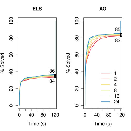
Figure 13: Performance profiles for PDFS.

Figure 13 shows performance profiles demonstrating how performance with PDFS varied across the range of threads used. Similar to the profiles for PA*, both models see an increase of 2-3% of problem instances solved with the use of parallelisation, after 120 seconds have elapsed. However, the absolute performance of AO is much better than that of ELS: AO solves more than twice as many problem instances within the time limit. Interestingly, DFBnB shows itself to be competitive with A* when used with the AO model, with almost the same proportion of problem instances solved. This is remarkable, as under the ELS model DFBnB is not performance competitive with A* [21]. This can also be observed when comparing Figure 10 with Figure 13, where we see that the single threaded PA*-DD under the ELS model (ELS(DD)) performs significantly better than any PDFS under ELS. In general, it is clear that performance with the AO model has scaled with the number of threads used in a similar manner as with PA*, but it is difficult to distinguish a trend in the ELS results.

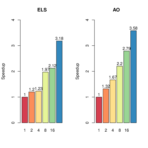
Figure 14: Speedup of PDFS at 60 seconds.

Figure 13 shows speedup calculated at 60 seconds for PDFS. Both ELS and AO show similar trends with speedup scaling consistently with the number of threads used. This view shows us that performance scales weakly, but consistently with the number of threads used for both state-space models, with ELS reaching a maximum speedup of 3.18 and AO reaching a maximum speedup of 3.58. Note that, unlike with PA*, the performance is not degraded when moving from 16 to 24 threads. This suggests that PDFS may continue to scale with higher numbers of threads before synchronisation overhead becomes too much.

5 Conclusions

A new state-space model for optimal task scheduling was recently proposed, in which duplicate states are not produced. This state-space model is known as AO, or Allocation-Ordering. We expected that this would be advantageous to a wide variety of branch-and-bound methods, in particular depth-first branch-and-bound and parallel algorithms. We have therefore investigated and proposed DFBnB and parallel search algorithms for optimal task scheduling. This includes a parallel algorithm based on A* (PA*) and one based on DFBnB (PDFS).

It was hypothesised that memory-limited search, such as with DFBnB, would produce better results with AO than with ELS, an older state-space model with many duplicate states. Our extensive experimental evaluation showed that AO was greatly superior to ELS when used with DFBnB, solving between 50% and 90% more problem instances within the time limit.

It was also considered likely that the lack of duplicates would allow parallel branch-and-bound to scale better with AO than with ELS, as the lack of data structures associated with duplicate detection would mean lower levels of synchronisation. The experimental evaluation of our proposed algorithms demonstrated that AO allowed the performance of parallel A* and DFBnB algorithms to scale better with the number of threads used, with problems that took the sequential algorithm 60 seconds being solved up to 3.58 times faster. While the scaling was not very strong, it was encouraging that it was consistent over a good number of threads.

A combination of comparable absolute performance, more consistent scaling in parallel, and the memory-limited nature of the DFBnB algorithm suggest that PDFS with the AO model is the best candidate method for optimal task scheduling with state-space search. This is a new result, as so far A* (using the ELS model) was superior to DFBnB.

References

- [1] B. Veltman, B. J. Lageweg, and J. K. Lenstra, “Multiprocessor Scheduling with Communication Delays,” Parallel Computing, vol. 16, no. 2-3, pp. 173–182, 1990.
- [2] V. Sarkar, Partitioning and scheduling parallel programs for multiprocessors. MIT press, 1989.
- [3] T. Hagras and J. Janecek, “A high performance, low complexity algorithm for compile-time task scheduling in heterogeneous systems,” Parallel Computing, vol. 31, no. 7, pp. 653–670, 2005.
- [4] T. Yang and A. Gerasoulis, “List scheduling with and without communication delays,” Parallel Computing, vol. 19, no. 12, pp. 1321–1344, 1993.
- [5] J.-J. Hwang, Y.-C. Chow, F. D. Anger, and C.-Y. Lee, “Scheduling Precedence Graphs in Systems with Interprocessor Communication Times,” SIAM J. Comput., vol. 18, no. 2, pp. 244–257, 1989.
- [6] O. Sinnen, Task Scheduling for Parallel Systems (Wiley Series on Parallel and Distributed Computing). Wiley-Interscience, 2007.
- [7] H. Wang and O. Sinnen, “List-scheduling vs. cluster-scheduling,” IEEE Transactions on Parallel and Distributed Systems, 2018.
- [8] M. Drozdowski, Scheduling for Parallel Processing. Springer Publishing Company, Incorporated, 1st ed., 2009.
- [9] A. Z. Semar Shahul and O. Sinnen, “Scheduling task graphs optimally with A*,” Journal of Supercomputing, vol. 51, pp. 310–332, Mar. 2010.
- [10] M. Orr and O. Sinnen, “A duplicate-free state-space model for optimal task scheduling,” in Proc. of 21st Int. European Conference on Parallel and Distributed Computing (Euro-Par 2015), vol. 9233 of Lecture Notes in Computer Science, (Vienna, Austria), Springer, 2015.
- [11] M. Orr and O. Sinnen, “Further explorations in state-space search for optimal task scheduling,” in 2017 IEEE 24th International Conference on High Performance Computing (HiPC), pp. 134–141, IEEE, 2017.
- [12] A. Krämer, “Branch and bound methods for scheduling problems with multiprocessor tasks on dedicated processors,” Operations-Research-Spektrum, vol. 19, no. 3, pp. 219–227, 1997.
- [13] S. Fujita, “A branch-and-bound algorithm for solving the multiprocessor scheduling problem with improved lower bounding techniques,” IEEE Transactions on computers, vol. 60, no. 7, pp. 1006–1016, 2011.
- [14] Y.-K. Kwok and I. Ahmad, “On multiprocessor task scheduling using efficient state space search approaches,” Journal of Parallel and Distributed Computing, vol. 65, no. 12, pp. 1515–1532, 2005.
- [15] O. Sinnen, “Reducing the solution space of optimal task scheduling,” Computers & Operations Research, vol. 43, no. 0, pp. 201 – 214, 2014.
- [16] A. A. El Cadi, R. B. Atitallah, S. d. Hanafi, N. Mladenović, and A. Artiba, “New mip model for multiprocessor scheduling problem with communication delays,” Optimization Letters, pp. 1–17, 2014.
- [17] S. Mallach, “Improved mixed-integer programming models for multiprocessor scheduling with communication delays,” 2016.
- [18] S. Venugopalan and O. Sinnen, “Integer linear programming for the multiprocessor scheduling problem with communication delays,” IEEE Transactions on Parallel and Distributed Systems, vol. 16, no. 1, pp. 142–151, 2015.
- [19] W. Zhang, State-space search: Algorithms, complexity, extensions, and applications. Springer Science & Business Media, 1999.
- [20] D. L. Poole and A. K. Mackworth, Artificial Intelligence: foundations of computational agents. Cambridge University Press, 2010.
- [21] S. Venugopalan and O. Sinnen, “Memory limited algorithms for optimal task scheduling on parallel systems,” Journal of Parallel and Distributed Computing, vol. 92, pp. 35–49, 2016.
- [22] A. Fukunaga, A. Botea, Y. Jinnai, and A. Kishimoto, “Parallel a* for state-space search,” in Handbook of Parallel Constraint Reasoning, pp. 419–455, Springer, 2018.
- [23] T. K. Ralphs, L. Ladányi, and M. J. Saltzman, “A library hierarchy for implementing scalable parallel search algorithms,” The Journal of Supercomputing, vol. 28, no. 2, pp. 215–234, 2004.
- [24] D. J. Challou, M. Gini, and V. Kumar, “Parallel search algorithms for robot motion planning,” in Robotics and Automation, 1993. Proceedings., 1993 IEEE International Conference on, pp. 46–51, IEEE, 1993.
- [25] A. Grama and V. Kumar, “Parallel search algorithms for discrete optimization problems,” ORSA Journal on Computing, vol. 7, no. 4, pp. 365–385, 1995.
- [26] E. Burns, S. Lemons, W. Ruml, and R. Zhou, “Best-first heuristic search for multicore machines,” Journal of Artificial Intelligence Research, vol. 39, pp. 689–743, 2010.
- [27] Y. Jinnai and A. Fukunaga, “Abstract zobrist hashing: An efficient work distribution method for parallel best-first search,” in Thirtieth AAAI Conference on Artificial Intelligence, 2016.
- [28] A. Bundy and L. Wallen, “Branch-and-bound algorithms,” in Catalogue of Artificial Intelligence Tools (A. Bundy and L. Wallen, eds.), Symbolic Computation, pp. 12–12, Springer Berlin Heidelberg, 1984.
- [29] N. J. N. P. E. Hart and B. Raphael, “A formal basis for the heuristic determination of minimum cost paths,” IEEE Transactions on Systems, Science, and Cybernetics, vol. SSC-4, no. 2, pp. 100–107, 1968.
- [30] A. Gerasoulis and T. Yang, “A comparison of clustering heuristics for scheduling directed acyclic graphs on multiprocessors,” Journal of Parallel and Distributed Computing, vol. 16, no. 4, pp. 276–291, 1992.
- [31] H. Kanemitsu, M. Hanada, and H. Nakazato, “Clustering-based task scheduling in a large number of heterogeneous processors,” IEEE Transactions on Parallel and Distributed Systems, vol. 27, no. 11, pp. 3144–3157, 2016.
- [32] W. Liu, H. Li, W. Du, and F. Shi, “Energy-aware task clustering scheduling algorithm for heterogeneous clusters,” in Proceedings of the 2011 IEEE/ACM International Conference on Green Computing and Communications, pp. 34–37, IEEE Computer Society, 2011.
- [33] M. Orr and O. Sinnen, “Optimal Task Scheduling Benefits From a Duplicate-Free State-Space,” arXiv e-prints, p. arXiv:1901.06899, Jan. 2019.
- [34] R. Crainic, Lecun, “Parallel branch-and-bound algorithms,” in Parallel combinatorial optimization (E.-G. Talbi, ed.), vol. 58, John Wiley & Sons, 2006.
- [35] A. Ioannou and M. G. Katevenis, “Pipelined heap (priority queue) management for advanced scheduling in high-speed networks,” IEEE/ACM Transactions on Networking (ToN), vol. 15, no. 2, pp. 450–461, 2007.
- [36] J. Lindén and B. Jonsson, “A skiplist-based concurrent priority queue with minimal memory contention,” in International Conference On Principles Of Distributed Systems, pp. 206–220, Springer, 2013.
- [37] R. D. Blumofe and C. E. Leiserson, “Scheduling multithreaded computations by work stealing,” Journal of the ACM (JACM), vol. 46, no. 5, pp. 720–748, 1999.
- [38] M. Frigo, C. E. Leiserson, and K. H. Randall, “The implementation of the cilk-5 multithreaded language,” ACM Sigplan Notices, vol. 33, no. 5, pp. 212–223, 1998.