Finite-time ruin probabilities under large-claim reinsurance treaties for heavy-tailed claim sizes

Abstract

We investigate the probability that an insurance portfolio gets ruined within a finite time period under the assumption that the $r$ largest claims are (partly) reinsured. We show that for regularly varying claim sizes the probability of ruin after reinsurance is also regularly varying in terms of the initial capital, and derive an explicit asymptotic expression for the latter. We establish this result by leveraging recent developments on sample/path large deviations for heavy tails. Our results allow, on the asymptotic level, for an explicit comparison between two well/known large/claim reinsurance contracts, namely LCR and ECOMOR. We finally assess the accuracy of the resulting approximations using state/of/the/art rare event simulation techniques.

1 Introduction

We consider the following ruin problem of the classical Cramér/Lundberg model in risk theory; see e.g. [4]. Let $\{X_{1},X_{2},\dots\}$ be a sequence of i.i.d. positive random variables representing successive claim sizes that arrive according to a homogeneous Poisson process $N(t)$, $t\geq 0$, with rate $\lambda$. Premiums are received continuously at a constant rate $p>\lambda\mathds{E}X$. We assume that there is also a reinsurance agreement in place, where $R(t)$ is the reinsured amount at time $t$. More precisely, if $S(t)=\sum_{i=1}^{N(t)}X_{i}$ is the aggregate claim amount at time $t$ and $p_{D}$ is the remaining premium for the insurer after reinsurance has been purchased, then the aggregate loss minus premiums at time $t$ for the insurer is equal to $S(t)-p_{D}t-R(t)$. If $u\geq 0$ is the initial capital, then the probability of ruin before time $T$ is defined as

$$\psi(u,T)=\mathds{P}\Bigg{(}\sup_{0\leq t\leq T}\{S(t)-p_{D}t-R(t)\}>u\Bigg{)}.$$ (1)

We will restrict our attention to two forms of large claims reinsurance, namely LCR and ECOMOR. In an LCR (largest claim reinsurance) contract (see e.g. [3] for an early reference), the reinsurer agrees to cover the largest $r$ claims, where $r\geq 1$ is a fixed number, while in an ECOMOR (excédent du coût moyen relatif) contract [19], the reinsurer covers the excess of the $r$ largest claims over the $(r+1)$st largest claim; see [2] for more details on this type of reinsurance contracts.

We assume that the distribution of the claim sizes belongs to a class of distributions with a regularly varying tail, which is valid for many applications [11]. It is well known that the principle of one big jump holds in the heavy/tailed claim setting, i.e. ruin is typically caused by a single large claim. However, under the presence of large claim reinsurance contracts, ruin probabilities are typically harder to analyse because the largest claims are covered by the reinsurer and thus multiple claims may be responsible for the event of ruin.

Several papers have studied properties of large claim reinsurance contracts. For example, when claim sizes are light/tailed, the asymptotic tail behavior of the reinsured amounts is considered in [12, 13] and their joint tail behavior in [17]. For asymptotic properties of the reinsured amounts when the claim size distribution is heavy/tailed, see [1, 15]. For dependence between claim sizes and interarrival times in this context, see [16]. An interesting recent link between large claim treaties and risk measures is given in [8]. However, none of these contributions deal with the ruin probability, which is considered here.

In this paper, we suggest to leverage recent new tools developed in the context of sample/path large deviations for heavy/tailed stochastic processes for the study of ruin problems under LCR and ECOMOR treaties. Concretely, for a centered Lévy process $Y(t)$, $t\geq 0$, with regularly varying Lévy measure $\nu$, sample/path large deviations were developed in [18]. Consider the process $\bar{Y}_{n}=\{\bar{Y}_{n}(t),t\in[0,1]\}$, where $\bar{Y}_{n}(t)=Y(nt)/n$, $t\geq 0$. Then, asymptotic estimates of $\mathds{P}(\bar{Y}_{n}\in A)$ for a large collection of sets $A$ were derived. For Lévy processes with only positive jumps that are regularly varying with index $-\alpha$, $\alpha>1$, these results take the form

$$C_{\mathcal{J}(A)}({A}^{\circ})\leq\liminf_{n\to\infty}\frac{\mathds{P}(\bar{Y}_{n}\in A)}{\big{(}n\cdot\nu[n,\infty)\big{)}^{\mathcal{J}(A)}}\leq\limsup_{n\to\infty}\frac{\mathds{P}(\bar{Y}_{n}\in A)}{\big{(}n\cdot\nu[n,\infty)\big{)}^{\mathcal{J}(A)}}\leq C_{\mathcal{J}(A)}(\bar{A}),$$ (2)

where ${A}^{\circ}$ and $\bar{A}$ are the interior and closure of $A$, $\mathcal{J}(A)$ is interpreted as the minimum number of jumps in the Lévy process that are needed to cause the event $A$, and $C_{j}$ is a measure. We will show how the reinsurance problem fits in the above framework. For this, we resolve several technical challenges such as showing how ruin probabilities in the reinsurance setting can be written as continuous maps of the input process in a suitable Skorokhod space.

Apart from the fact that reinsurance contracts are an interesting object of study in their own right, the present application seems to be the first example for which it is possible to compute the pre/factors in the asymptotics (2) explicitly. More precisely, we show for both the LCR and ECOMOR treaty that $C_{\mathcal{J}(A)}({A}^{\circ})=C_{\mathcal{J}(A)}(\bar{A})$ and we provide an explicit expression for this value.

The rest of the paper is organised as follows. In Section 2, we provide some preliminary results and introduce the necessary notation. Section 3 develops the main result, i.e. the tail asymptotics for finite time ruin probabilities. For this, we are inquired to write (1) in terms of (2). This leads to the need to show continuity of certain mappings, as well as several additional technical requirements. In Section 4, we validate our asymptotic results with numerical experiments.

2 Model description and preliminaries

Following the notation and terminology used in Section 1, let $F$ denote the distribution function of the claim sizes and $\mathds{E}X$ be their expectation. We assume that $F$ is regularly varying with index $-\alpha$, i.e. there exists a slowly varying function $L(x)$ such that $\bar{F}(x):=1-F(x)=L(x)x^{-\alpha}$, with $\alpha>1$. Let further $X^{\star}_{1,N(t)}\geq X^{\star}_{2,N(t)}\geq\cdots\geq X^{\star}_{N(t),N(t)}$ denote the order statistics of $X_{1},X_{2},\dots X_{N(t)}$.

In an LCR treaty, the reinsured amount $R(t)$ is equal to

$$L_{r}(t):=\sum_{i=1}^{r}X^{\star}_{i,N(t)},$$ (3)

i.e. the $r$ largest claims are paid by the reinsurer. On the other hand, the reinsured amount $R(t)$ in an ECOMOR treaty takes the form

$$E_{r}(t):=\sum_{i=1}^{r}X^{\star}_{i,N(t)}-rX^{\star}_{r+1,N(t)}=\sum_{i=1}^{N(t)}\big{(}X_{i}-X^{\star}_{r+1,N(t)}\big{)}_{+}.$$ (4)

That is, the ECOMOR constitutes an excess/of/loss treaty with a random retention, and the latter is the $(r+1)$-largest claim. For more details and background on such reinsurance contracts, see [2]. In either treaty, the number of reinsured claims is equal to $r$.

Assumption 1.

If $N(t)\leq r$, we set $X^{\star}_{i,N(t)}=0$, for $i=N(t)+1,\dots,r+1$. This means that in case there are less than $r+1$ claims, the reinsurer pays all the claims in the ECOMOR treaty.

Another modeling assumption is concerned with the way the reinsurance is affecting the capital position of the insurance company under consideration.

Assumption 2.

We assume that at each time $t$, the currently applicable reinsured amount $R(t)$ is considered in the determination of the available surplus. In particular, this means that before the arrival of the $(r+1)$-st claim, the random retention in the ECOMOR treaty is considered to be zero. As a consequence in the ECOMOR treaty, the arrival of a new claim can lead to a modification of $R(t)$ of either sign, as the excess over the $(r+1)$-st claim may also decrease.

Note also that the setup we study here is that the duration of the reinsurance contract is $T$, and the implied premium for the reinsurance contract over the period $[0,T]$ is uniformly spread over this time interval. We will study the asymptotic behavior of the finite time ruin probabilities (1) utilizing (2). Therefore, we formulate in the next section the large deviation problem that arises in our reinsurance context.

2.1 Large deviations in reinsurance

In [18], the large deviations results (2) were derived in the Skorokhod $J_{1}$ topology. Correspondingly, we let $\mathds{D}=\mathds{D}([0,1],\mathds{R})$ be a Skorokhod space, i.e. a space of real/valued càdlàg (right continuous with left limits) functions on $[0,1]$, equipped with the $J_{1}$-metric defined by

$$d(\xi,\zeta)=\inf_{h\in\Lambda}\{\|h-id\|\vee\|\xi-\zeta\circ h\|\},\qquad(\xi,\zeta)\in\mathds{D}^{2},$$ (5)

where $\Lambda$ denotes the set of all strictly increasing continuous bijections from $[0,1]$ to itself, $id$ denotes the identity mapping, and $\|\cdot\|$ denotes the uniform (sup) norm on $[0,1]$. Thus, $A$ and $C_{j}$ in (2) are a measurable set and a measure on $\mathds{D}$, respectively. Furthermore, if $\phi:\mathds{D}\to\mathds{R}$ is a continuous functional on $\mathds{D}$ and $B\in\mathcal{B}(\mathds{R})$ is a Borel set such that $A=\phi^{-1}(B)$, where $\phi^{-1}$ stands for the inverse of $\phi$, it holds that

$$\mathds{P}\big{(}\phi(\bar{Y}_{n})\in B\big{)}=\mathds{P}\big{(}\bar{Y}_{n}\in\phi^{-1}(B)\big{)}=\mathds{P}(\bar{Y}_{n}\in A).$$ (6)

The above relation portrays how it is possible to use the result (2) to study continuous functionals of $\bar{Y}_{n}$. To connect this to our ruin problem, we define $\bar{S}_{n}:=\{\bar{S}_{n}(t),t\in[0,1]\}$ as the centred and scaled process

$$\bar{S}_{n}(t)=\frac{1}{n}S(nt)-\lambda\mathds{E}Xt=\frac{1}{n}\sum_{i=1}^{N(nt)}X_{i}-\lambda\mathds{E}Xt,\quad t\geq 0.$$ (7)

Moreover, we assume that the capital $u$ increases linearly in $n$, i.e. there exists an $a>0$ such that $u=na$. We now formulate the large deviations problem to estimate the probabilities

$$\mathds{P}\Bigg{(}\sup_{t\in[0,1]}\{S(nt)-p_{D}nt-R(nt)\}\geq na\Bigg{)}$$

$$=\mathds{P}\Bigg{(}\sup_{t\in[0,1]}\{S(nt)-\lambda\mathds{E}Xnt-(p_{D}-\lambda\mathds{E}X)nt-R(nt)\}\geq na\Bigg{)}$$

$$=\mathds{P}\Bigg{(}\sup_{t\in[0,1]}\{n\bar{S}_{n}(t)-cnt-R(nt)\}\geq na\Bigg{)}=\mathds{P}\Bigg{(}\sup_{t\in[0,1]}\{\bar{S}_{n}(t)-ct-\frac{1}{n}R(nt)\}\geq a\Bigg{)},$$ (8)

where $c=p_{D}-\lambda\mathds{E}X$. As a next step, we must identify a continuous functional $\phi$ such that

$$\sup_{t\in[0,1]}\{\bar{S}_{n}(t)-ct-\frac{1}{n}R(nt)\}=\phi(\bar{S}_{n}),$$ (9)

so that we can write

$$\mathds{P}\Bigg{(}\sup_{t\in[0,1]}\{\bar{S}_{n}(t)-ct-\frac{1}{n}R(nt)\}\geq a\Bigg{)}=\mathds{P}\big{(}\phi(\bar{S}_{n})\geq a\big{)}=\mathds{P}\Big{(}\bar{S}_{n}\in\phi^{-1}\big{(}[a,\infty)\big{)}\Big{)}.$$ (10)

However, it is not immediately obvious from Equation 9 what the functional $\phi$ looks like because $R(nt)$ is not expressed in terms of $\bar{S}_{n}$. We focus first on the LCR treaty and observe that

$$\frac{1}{n}R(nt)=\frac{1}{n}L_{r}(nt)=\frac{1}{n}\sum_{i=1}^{r}X^{\star}_{i,N(nt)}=\max_{\begin{subarray}{c}(s_{1},\dots,s_{r})\in[0,t]^{r}\\ s_{i}\neq s_{j},\forall i\neq j\end{subarray}}\sum_{i=1}^{r}\big{(}\bar{S}_{n}(s_{i})-\bar{S}_{n}(s_{i}^{-})\big{)},\quad t\in[0,1],$$

i.e. $L_{r}(nt)/n$ can be expressed as the sum of the $r$ biggest jumps of the process $\bar{S}_{n}(t)$. For every $\xi\in\mathds{D}$ and $m\in\mathds{N}$, we define

$${\mathfrak{J}}^{m}_{\xi}(t)=\sup_{\begin{subarray}{c}(s_{1},\dots,s_{m})\in[0,t]^{m}\\ s_{i}\neq s_{j},\forall i\neq j\end{subarray}}\sum_{i=1}^{m}\big{(}\xi(s_{i})-\xi(s_{i}^{-})\big{)}=\max_{\begin{subarray}{c}(s_{1},\dots,s_{m})\in[0,t]^{m}\\ s_{i}\neq s_{j},\forall i\neq j\end{subarray}}\sum_{i=1}^{m}\big{(}\xi(s_{i})-\xi(s_{i}^{-})\big{)},\quad\text{for }t\in(0,1],$$ (11)

as the supremum of the sum of the $m$ largest jumps of the function $\xi$. Naturally, ${\mathfrak{J}}^{m}_{\xi}(0)=0$. Consequently, the functional $\phi$ we are looking for is a mapping $\phi_{r}:\mathds{D}\to\mathds{R}$ defined for every $\xi\in\mathds{D}$ as

$$\phi_{r}(\xi)=\sup_{t\in[0,1]}\Big{\{}\xi(t)-ct-{\mathfrak{J}}^{r}_{\xi}(t)\Big{\}}.$$ (12)

Moreover, we denote the pre/image of $[a,\infty)$ under $\phi_{r}$ as $A^{r}_{c,a}=\phi_{r}^{-1}\big{(}[a,\infty)\big{)}$ where

$$A^{r}_{c,a}=\Bigg{\{}\xi\in\mathds{D}:\sup_{t\in[0,1]}\Big{\{}\xi(t)-ct-{\mathfrak{J}}^{r}_{\xi}(t)\Big{\}}\geq a\Bigg{\}}.$$ (13)

By comparing Equations 3 and 4, we observe that the relation between the reinsured amounts of the two treaties is

$$E_{r}(t)=L_{r}(t)-rX^{\star}_{r+1,N(t)}=(r+1)L_{r}(t)-r\big{(}L_{r}(t)+X^{\star}_{r+1,N(t)}\big{)}=(r+1)L_{r}(t)-rL_{r+1}(t).$$

Thus, in the ECOMOR treaty, the functional $\phi$ in (10) is the mapping $\varphi_{r}:\mathds{D}\to\mathds{R}$ defined for every $\xi\in\mathds{D}$ as

$$\varphi_{r}(\xi)=\sup_{t\in[0,1]}\Big{\{}\xi(t)-ct-(r+1){\mathfrak{J}}^{r}_{\xi}(t)+r{\mathfrak{J}}^{r+1}_{\xi}(t)\Big{\}},$$ (14)

while the pre/image of $[a,\infty)$ under $\varphi_{r}$, i.e. $\mathcal{A}^{r}_{c,a}=\varphi_{r}^{-1}\big{(}[a,\infty)\big{)}$, is defined as

$$\mathcal{A}^{r}_{c,a}=\Bigg{\{}\xi\in\mathds{D}:\sup_{t\in[0,1]}\Big{\{}\xi(t)-ct-(r+1){\mathfrak{J}}^{r}_{\xi}(t)+r{\mathfrak{J}}^{r+1}_{\xi}(t)\Big{\}}\geq a\Bigg{\}}.$$ (15)

2.2 Preliminaries on the Skorokhod topology and notation

Consider the complete metric space $\big{(}\mathds{D},d(,)\big{)}$. The functional ${\mathfrak{J}}^{m}_{\xi}(t)$ defined in (11) will play a significant role in the forthcoming analysis. Thus, it is important to confirm that it is well/defined. For this reason, let $\mathcal{D}(\xi)$ be the set of discontinuities of $\xi\in\mathds{D}$, i.e.

$$\mathcal{D}(\xi)=\{t\in[0,1]:\xi(t^{-})\neq\xi(t)\},$$ (16)

and let $\mathcal{D}(\xi,\epsilon)$ be the set of discontinuities of magnitude at least $\epsilon$, i.e.

$$\mathcal{D}(\xi,\epsilon)=\{t\in[0,1]:\left|{\xi(t^{-})-\xi(t)}\right|\geq\epsilon\}.$$ (17)

The following result is standard.

Lemma 2.1 (Theorem 12.2.1 & Corollary 12.2.1 of [20]).

For any $\xi\in\mathds{D}$ and $\epsilon>0$, $\mathcal{D}(\xi,\epsilon)$ is a finite subset of $[0,1]$. In particular, $\mathcal{D}(\xi)$ is either finite or countably infinite.

Consequently, the supremum in Equation 11 is attained because only finitely many jumps can exceed a given positive number. As a result, ${\mathfrak{J}}^{m}_{\xi}(t)$ is well defined.

Some important subspaces of $\mathds{D}$ for our analysis are those restricted to step functions. We let $\mathds{D}^{\uparrow}_{\mathcal{S}}$ be the set of all non/decreasing step functions vanishing at the origin. Furthermore, $\mathds{D}_{j}$ is the subspace of $\mathds{D}$ consisting of non/decreasing step functions, vanishing at the origin, with exactly $j$ steps, and similarly, $\mathds{D}_{\leqslant j}=\bigcup_{0\leq i\leq j}\mathds{D}_{i}$ consists of non/decreasing step functions, vanishing at the origin, with at most $j$ steps. Finally, if $\mathcal{D}_{+}(\xi)$ denotes the number of discontinuities of $\xi\in\mathds{D}$, we can then formally define the integer/valued set function $\mathcal{J}(A)$ appearing in Equation 2 by:

$$\mathcal{J}(A)=\inf_{\xi\in A\cap\mathds{D}^{\uparrow}_{\mathcal{S}}}\mathcal{D}_{+}(\xi),$$ (18)

which we call the rate function. Observe that every $\xi\in\mathds{D}_{j}$ is determined by the pair of jump sizes and jump times $(\bm{{x}},\bm{{u}})\in\mathds{R}^{j}_{+}\times[0,1]^{j}$, i.e. $\xi(t)=\sum_{i=1}^{j}x_{i}\mathds{1}_{\{u_{i},1\}}(t)$, where $\mathds{1}_{B}$ is the indicator function on the set $B$. For $\bm{{x}}=(x_{1},\dots,x_{j})$ and $\bm{{u}}=(u_{1},\dots,u_{j})$, we define the sets

$$\mathds{R}^{j\downarrow}_{+} =\{\bm{{x}}\in\mathds{R}^{j}_{+}:x_{1}\geq x_{2}\geq\dots\geq x_{j}>0\},$$ (19)

and

$$S_{j} =\{(\bm{{x}},\bm{{u}})\in\mathds{R}^{j\downarrow}_{+}\times(0,1)^{j}:u_{1},\dots,u_{j}\text{ are all distinct}\},$$ (20)

where the $u_{j}$’s are not following the ordering of the $x_{j}$’s, i.e. $x_{k}\geq x_{l}\not\Rightarrow u_{k}\geq u_{l}$. Thus, we can formally define the mapping $T_{j}:S_{j}\to\mathds{D}_{j}$ by $T_{j}(\bm{{x}},\bm{{u}})=\sum_{i=1}^{j}x_{i}\mathds{1}_{\{u_{i},1\}}$.

Furthermore, let $\nu_{\alpha}(x,\infty)=x^{-\alpha}$ (i.e. the pure power decay part of the regularly varying claim sizes), and let $\nu^{j}_{\alpha}$ denote the restriction to $\mathds{R}^{j\downarrow}_{+}$ of the $j$/fold product measure of $\nu_{\alpha}$. We define for each $j\geq 1$ the measure $C_{j}$ concentrated on $\mathds{D}_{j}$ as

$$C_{j}(\bullet)=\mathds{E}\big{[}\nu^{j}_{\alpha}\{\bm{{y}}\in\mathds{R}^{j}_{+}:\sum_{i=1}^{j}y_{i}\mathds{1}_{\{U_{i},1\}}\in\bullet\}\big{]},$$ (21)

where the random variables $U_{i}$, $i=1,\dots,j$, are i.i.d. uniform on $[0,1]$.

Finally, we say that a set $A\subseteq\mathds{D}$ is bounded away from another set $B\subseteq\mathds{D}$ if $\inf_{x\in A,y\in B}d(x,y)>0$. Additionally, we let $\prescript{}{\delta}{A}=\{\xi\in\mathds{D}:d(\xi,A)\leq\delta\}$ for any $\delta>0$.

3 Main result

Note that the parameter $c=p_{D}-\lambda\mathds{E}X$ introduced in Section 2.1 can be either positive or negative. However, for $a\leq-c$, the rare event probability in Equation 10 converges to one by the functional law of large numbers. For this reason, we focus only on the case $c+a>0$. Letting $\displaystyle\prescript{}{2}{F}_{1}(b,e;d;z)=\sum_{k=0}^{+\infty}\frac{(b)_{k}(e)_{k}}{(d)_{k}}\frac{z^{k}}{k!}$ be the hypergeometric function, with $(b)_{k}=b(b+1)\dots(b+k-1)$ denoting the Pochhammer symbol, we have the following theorem.

Theorem 3.1.

For $a>0$, $c+a>0$, and $r\in\mathds{N}$, it holds that

$$\psi(na,n)\sim\mathcal{C}_{r+1}\big{(}\lambda L(n)\big{)}^{r+1}n^{-(r+1)(\alpha-1)},\qquad n\to\infty,$$ (22)

where

$$\mathcal{C}_{r+1}=\Bigg{[}a^{-(r+1)\alpha}\prescript{}{2}{F}_{1}[r+1,(r+1)\alpha;r+2;-c/a]\cdot\mathds{1}_{\{c>0\}}+(a+c)^{-(r+1)\alpha}\cdot\mathds{1}_{\{c<0\}}\Bigg{]}\times\frac{1}{(r+1)!}$$

$$\times\begin{cases}1,&\text{if }R(t)=L_{r}(t)\text{ (LCR)},\\ (r+1)^{(r+1)\alpha},&\text{if }R(t)=E_{r}(t)\text{ (ECOMOR)}.\end{cases}$$

The proof of Theorem 3.1 is based on sample/path large/deviations results developed in [18]. Specifically, Theorems 3.1–3.2 in [18] provide the conditions under which the result (2) holds, and in addition the $\liminf$ and $\limsup$ are equal. Thus, to achieve our goal, we must verify that these conditions are satisfied for $\bar{Y}_{n}=\bar{S}_{n}$ and $A=A^{r}_{c,a}$ (LCR) or $A=\mathcal{A}^{r}_{c,a}$ (ECOMOR) defined in Equations 13 and 15, respectively. However, their verification is rather involved. Hence, to make the proof of Theorem 3.1 more accessible, we split it in various steps after the aforementioned conditions and we provide additional explanations for each step.

Note that all of the forthcoming results are similar in the two treaties with possible deviations in small details. Therefore, we will first prove them for the LCR treaty and then show briefly how they can be extended to the ECOMOR treaty.

3.1 Proof of Theorem 3.1

The first step is to show that both mappings $\phi_{r},\varphi_{r}:\mathds{D}\to\mathds{R}$ from Equations 12 and 14, respectively, are Lipschitz continuous. Due to their continuity, Equation 10 will hold and, consequently, we will be able to write $\mathds{P}\big{(}\phi_{r}(\bar{S}_{n})\geq a\big{)}=\mathds{P}(\bar{S}_{n}\in A^{r}_{c,a})$ and $\mathds{P}\big{(}\varphi_{r}(\bar{S}_{n})\geq a\big{)}=\allowbreak\mathds{P}(\bar{S}_{n}\in\mathcal{A}^{r}_{c,a})$. For this, we need the following intermediate result.

Lemma 3.2.

For every $(\xi,\zeta)\in\mathds{D}^{2}$, $m\in\mathds{N}$, and $h\in\Lambda$, it holds that

$$\left|{{\mathfrak{J}}^{m}_{\zeta\circ h}(t)-{\mathfrak{J}}^{m}_{\xi}(t)}\right|\leq 2m\|\xi-\zeta\circ h\|,\qquad\forall t\in[0,1].$$ (23)

Proof.

By the definition of ${\mathfrak{J}}^{m}_{\zeta\circ h}(t)$, there exists $(\sigma_{1},\dots,\sigma_{m})\in[0,t]^{m}$ with $\sigma_{i}\neq\sigma_{j}$ for all $i\neq j$, such that

$${\mathfrak{J}}^{m}_{\zeta\circ h}(t)=\sum_{i=1}^{m}\big{(}\zeta\circ h(\sigma_{i})-\zeta\circ h(\sigma_{i}^{-})\big{)}.$$ (24)

In addition, we have that

$${\mathfrak{J}}^{m}_{\xi}(t)=\max_{\begin{subarray}{c}(s_{1},\dots,s_{m})\in[0,t]^{m}\\ s_{i}\neq s_{j},\forall i\neq j\end{subarray}}\sum_{i=1}^{m}\big{(}\xi(s_{i})-\xi(s_{i}^{-})\big{)}\geq\sum_{i=1}^{m}\big{(}\xi(\sigma_{i})-\xi(\sigma_{i}^{-})\big{)}.$$ (25)

Subtracting now Equations 24 and 25, we obtain

$${\mathfrak{J}}^{m}_{\zeta\circ h}(t)-{\mathfrak{J}}^{m}_{\xi}(t) \leq\sum_{i=1}^{m}\big{(}\zeta\circ h(\sigma_{i})-\zeta\circ h(\sigma_{i}^{-})-\xi(\sigma_{i})+\xi(\sigma_{i}^{-})\big{)}$$

$$\leq\sum_{i=1}^{m}\big{(}\left|{\zeta\circ h(\sigma_{i})-\xi(\sigma_{i})}\right|+\left|{\zeta\circ h(\sigma_{i}^{-})-\xi(\sigma_{i}^{-})}\right|\big{)}$$

$$\leq 2m\|\xi-\zeta\circ h\|.$$

Following similar arguments, we can also show that ${\mathfrak{J}}^{m}_{\xi}(t)-{\mathfrak{J}}^{m}_{\zeta\circ h}(t)\leq 2m\|\xi-\zeta\circ h\|$, which completes the proof. ∎

We are now ready to establish the desired continuity.

Lemma 3.3 (Lipschitz continuity of the mapping).

The mappings $\phi_{r},\varphi_{r}:\mathds{D}\to\mathds{R}$ defined by Equations 12 and 14, respectively, are Lipschitz continuous w.r.t. $J_{1}$. More precisely, there exist $K\in[0,\left|{c}\right|+2r+1]$ and $L\in[0,\left|{c}\right|+4r^{2}+4r+1]$ such that $\left|{\phi_{r}(\xi)-\phi_{r}(\zeta)}\right|\leq Kd(\xi,\zeta)$ and $\left|{\varphi_{r}(\xi)-\varphi_{r}(\zeta)}\right|\leq Ld(\xi,\zeta)$, for all $(\xi,\zeta)\in\mathds{D}^{2}$.

Proof.

W.l.o.g. we assume that $\phi_{r}(\xi)\geq\phi_{r}(\zeta)$, otherwise we switch the roles of $\xi$ and $\zeta$. For every $\epsilon>0$, there exists $t_{*}\in[0,1]$ such that

$$\xi(t_{*})-ct_{*}-{\mathfrak{J}}^{r}_{\xi}(t_{*})>\phi_{r}(\xi)-\epsilon.$$ (26)

On the other hand, by the definition of $J_{1}$, there exists $h=h(\xi,\zeta,\epsilon)\in\Lambda$ so that

$$d(\xi,\zeta)+\epsilon=\|h-id\|\vee\|\xi-\zeta\circ h\|\geq\big{(}h(t_{*})-t_{*}\big{)}\vee\big{(}\xi(t_{*})-\zeta\circ h(t_{*})\big{)}.$$ (27)

Furthermore, using the fact that $h$ is a homeomorphism on $[0,1]$, we obtain

$$\zeta\circ h(t_{*})-ch(t_{*})-{\mathfrak{J}}^{r}_{\zeta\circ h}(t_{*})$$

$$=\zeta\circ h(t_{*})-ch(t_{*})-\max_{\begin{subarray}{c}(s_{1},\dots,s_{r})\in[0,t_{*}]^{r}\\ s_{i}\neq s_{j},\forall i\neq j\end{subarray}}\sum_{i=1}^{r}\big{(}\zeta\circ h(s_{i})-\zeta\circ h(s_{i}^{-})\big{)}$$

$$=\zeta\big{(}h(t_{*})\big{)}-ch(t_{*})-\max_{\begin{subarray}{c}(s_{1},\dots,s_{r})\in[0,h(t_{*})]^{r}\\ s_{i}\neq s_{j},\forall i\neq j\end{subarray}}\sum_{i=1}^{r}\big{(}\zeta(s_{i})-\zeta(s_{i}^{-})\big{)}$$

$$=\zeta\big{(}h(t_{*})\big{)}-ch(t_{*})-{\mathfrak{J}}^{r}_{\zeta}(h(t_{*}))\leq\phi_{r}(\zeta).$$ (28)

Subtracting (28) from (26) yields

$$\phi_{r}(\xi)-\phi_{r}(\zeta) <\epsilon+\big{(}\xi(t_{*})-\zeta\circ h(t_{*})\big{)}+c\big{(}h(t_{*})-t_{*}\big{)}+\big{(}{\mathfrak{J}}^{r}_{\zeta\circ h}(t_{*})-{\mathfrak{J}}^{r}_{\xi}(t_{*})\big{)}$$

$$<\epsilon+\big{(}d(\xi,\zeta)+\epsilon\big{)}+\left|{c}\right|\big{(}d(\xi,\zeta)+\epsilon\big{)}+2r\big{(}d(\xi,\zeta)+\epsilon\big{)}$$

$$=(2+\left|{c}\right|+2r)\epsilon+(1+\left|{c}\right|+2r)d(\xi,\zeta),$$

where we have also used (27) and ${\mathfrak{J}}^{r}_{\zeta\circ h}(t_{*})-{\mathfrak{J}}^{r}_{\xi}(t_{*})\leq 2r\|\xi-\zeta\circ h\|$ by applying Lemma 3.2 with $t=t_{*}$ and $m=r$. Letting $\epsilon\to 0$, we conclude that $\phi_{r}(\xi)-\phi_{r}(\zeta)\leq(1+\left|{c}\right|+2r)d(\xi,\zeta)$, i.e. $\phi_{r}$ is Lipschitz continuous. The Lipschitz continuity for the $\varphi_{r}$ mapping can be shown in an analogous manner. More precisely, for every $\epsilon>0$, there exists $t_{*}\in[0,1]$ such that

$$\xi(t_{*})-ct_{*}-(r+1){\mathfrak{J}}^{r}_{\xi}(t_{*})+r{\mathfrak{J}}^{r+1}_{\xi}(t_{*})>\varphi_{r}(\xi)-\epsilon.$$ (29)

For a homeomorphism $h$ on $[0,1]$ satisfying Equation 27, we have

$$\zeta\circ h(t_{*})-ch(t_{*})-(r+1){\mathfrak{J}}^{r}_{\zeta\circ h}(t_{*})+r{\mathfrak{J}}^{r+1}_{\zeta\circ h}(t_{*})$$

$$=\zeta\big{(}h(t_{*})\big{)}-ch(t_{*})-(r+1){\mathfrak{J}}^{r}_{\zeta}(h(t_{*}))+r{\mathfrak{J}}^{r+1}_{\zeta}(h(t_{*}))\leq\varphi_{r}(\zeta).$$ (30)

We assume now w.l.o.g. that $\varphi_{r}(\xi)\geq\varphi_{r}(\zeta)$ and we subtract (30) from (29) to attain

$$\varphi_{r}(\xi)-\varphi_{r}(\zeta)< \ \epsilon+\big{(}\xi(t_{*})-\zeta\circ h(t_{*})\big{)}+c\big{(}h(t_{*})-t_{*}\big{)}+(r+1)\big{(}{\mathfrak{J}}^{r}_{\zeta\circ h}(t_{*})-{\mathfrak{J}}^{r}_{\xi}(t_{*})\big{)}$$

$$+r\big{(}{\mathfrak{J}}^{r+1}_{\xi}(t_{*})-{\mathfrak{J}}^{r+1}_{\zeta\circ h}(t_{*})\big{)}$$

$$< \ \ \big{(}2+\left|{c}\right|+4r(r+1)\big{)}\epsilon+\big{(}1+\left|{c}\right|+4r(r+1)\big{)}d(\xi,\zeta),$$

where we have also used (27) and twice Lemma 3.2 with $m=r,r+1$ and $t=t_{*}$. Letting $\epsilon\to 0$, the result is immediate. ∎

As a next step, we calculate the rate functions $\mathcal{J}(A^{r}_{c,a})$ and $\mathcal{J}(\mathcal{A}^{r}_{c,a})$ that appear in Equation 2 and are formally defined in (18). We set for simplicity $c_{+}=\max\{0,c\}$ and $c_{-}=\max\{0,-c\}$.

Lemma 3.4 (Evaluation of the rate function).

The rate function defined by Equation 18 is equal to $r+1$ in both treaties, i.e.

$$\mathcal{J}(A^{r}_{c,a})=\mathcal{J}(\mathcal{A}^{r}_{c,a})=r+1.$$

Proof.

We need to show first that $\mathcal{J}(A^{r}_{c,a})$ cannot take any value smaller than or equal to $r$. Let us assume on the contrary that $\xi\in A^{r}_{c,a}\cap\mathds{D}^{\uparrow}_{\mathcal{S}}$ such that $\mathcal{D}_{+}(\xi)=k\leq r$. This means that $\xi=\sum_{i\leq k}x_{i}\mathds{1}_{\{u_{i},1\}}$, with $x_{1}\geq x_{2}\geq\dots x_{k}>0$ and $\{0,u_{1},u_{2},\dots,u_{k},1\}$ all distinct. By taking into account Assumptions 1 and 2, we calculate

$$\phi_{r}(\xi) =\sup_{t\in[0,1]}\Big{\{}\xi(t)-ct-{\mathfrak{J}}^{r}_{\xi}(t)\Big{\}}=\sup_{t\in[0,1]}\Big{\{}\cancel{\sum_{i=1}^{k}x_{i}\mathds{1}_{\{u_{i},1\}}(t)}-ct-\cancel{\sum_{i=1}^{k}x_{i}\mathds{1}_{\{u_{i},1\}}(t)}\Big{\}}=c_{-},$$

which states that $\xi\not\in A^{r}_{c,a}$ because $\phi_{r}(\xi)=c_{-}\not\geq a$. As a result, $\mathcal{J}(A^{r}_{c,a})\not=k$, $k\leq r$.

Let us assume now that $\xi\in A^{r}_{c,a}\cap\mathds{D}^{\uparrow}_{\mathcal{S}}$ such that $\mathcal{D}_{+}(\xi)=r+1$, i.e. $\xi=\sum_{i=1}^{r+1}x_{i}\mathds{1}_{\{u_{i},1\}}$, with $x_{1}\geq x_{2}\geq\dots x_{r+1}>0$ and $\{0,u_{1},u_{2},\dots,u_{r+1},1\}$ all distinct. To calculate $\phi_{r}(\xi)$, observe first that

$$\xi(t)-{\mathfrak{J}}^{r}_{\xi}(t)=\sum_{i=1}^{r+1}x_{i}\mathds{1}_{\{u_{i},1\}}(t)-{\mathfrak{J}}^{r}_{\xi}(t)=\begin{cases}0,&t<\max\{u_{1},\dots,u_{r+1}\}\\ x_{r+1},&t\geq\max\{u_{1},\dots,u_{r+1}\}\end{cases},$$ (31)

because all the claims are “absorbed” according to Assumption 2 before the arrival of the ($r+1$)st claim, which happens at time $t^{*}=\max\{u_{1},\dots,u_{r+1}\}$. Thus, we can write

$$\phi_{r}(\xi) =\sup_{t\in[0,1]}\Big{\{}\xi(t)-ct-{\mathfrak{J}}^{r}_{\xi}(t)\Big{\}}=\sup_{t\in[0,1]}\Big{\{}x_{r+1}\prod_{i=1}^{r+1}\mathds{1}_{\{u_{i},1\}}(t)-ct\Big{\}}$$

$$=x_{r+1}-c_{+}\max\{u_{1},\dots,u_{r+1}\}+c_{-},$$

since $x_{r+1}\prod_{i=1}^{r+1}\mathds{1}_{\{u_{i},1\}}(t)$ remains fixed at the value $x_{r+1}$ from $t^{*}=\max\{u_{1},\dots,u_{r+1}\}$ onward, while $-ct$ decreases or increases depending on the value of $c$. Due to the fact that $\xi\in A^{r}_{c,a}$, we get

$$\phi_{r}(\xi)\geq a\Rightarrow x_{r+1}\geq a+c_{+}\max\{u_{1},\dots,u_{r+1}\}-c_{-}\geq a-c_{-}>0,$$

i.e. $A^{r}_{c,a}\cap\mathds{D}^{\uparrow}_{\mathcal{S}}\not=\emptyset$ but contains all step functions with $r+1$ steps such that the ($r+1$)st largest step satisfies: $x_{r+1}\geq a+c_{+}\max\{u_{1},\dots,u_{r+1}\}-c_{-}$. Thus, $\mathcal{J}(A^{r}_{c,a})=r+1$.

The proof for $\mathcal{J}(\mathcal{A}^{r}_{c,a})=r+1$ in the ECOMOR treaty is similar. More precisely, it can easily be shown that $\not\exists\ \xi\in\mathcal{A}^{r}_{c,a}\cap\mathds{D}^{\uparrow}_{\mathcal{S}}$ with $\mathcal{D}_{+}(\xi)=k\leq r$. Consequently, $\mathcal{J}(\mathcal{A}^{r}_{c,a})\not=k$, $k\leq r$. Let us assume next that $\xi\in\mathcal{A}^{r}_{c,a}\cap\mathds{D}^{\uparrow}_{\mathcal{S}}$ such that $\mathcal{D}_{+}(\xi)=r+1$, i.e. $\xi=\sum_{i=1}^{r+1}x_{i}\mathds{1}_{\{u_{i},1\}}$, with $x_{1}\geq x_{2}\geq\dots x_{r+1}>0$ and $\{0,u_{1},u_{2},\dots,u_{r+1},1\}$ all distinct. It holds that

$$r{\mathfrak{J}}^{r+1}_{\xi}(t)-(r+1){\mathfrak{J}}^{r}_{\xi}(t)=-{\mathfrak{J}}^{r}_{\xi}(t)+\begin{cases}0,&t<\max\{u_{1},\dots,u_{r+1}\}\\ rx_{r+1},&t\geq\max\{u_{1},\dots,u_{r+1}\}\end{cases},$$ (32)

due to Assumption 1. By combining now Equations 31 and 32, we calculate

$$\varphi_{r}(\xi) =\sup_{t\in[0,1]}\Big{\{}\xi(t)-ct-(r+1){\mathfrak{J}}^{r}_{\xi}(t)+r{\mathfrak{J}}^{r+1}_{\xi}(t)\Big{\}}=\sup_{t\in[0,1]}\Big{\{}(r+1)x_{r+1}\prod_{i=1}^{r+1}\mathds{1}_{\{u_{i},1\}}(t)-ct\Big{\}}$$

$$=(r+1)x_{r+1}-c_{+}\max\{u_{1},\dots,u_{r+1}\}+c_{-}.$$

Since $\xi\in\mathcal{A}^{r}_{c,a}$, we get $\varphi_{r}(\xi)\geq a\Rightarrow(r+1)x_{r+1}\geq a+c_{+}\max\{u_{1},\dots,u_{r+1}\}-c_{-}$, i.e. $\mathcal{A}^{r}_{c,a}\cap\mathds{D}^{\uparrow}_{\mathcal{S}}\not=\emptyset$ but contains all step functions with $r+1$ steps such that the ($r+1$)st largest step satisfies: $x_{r+1}\geq\big{(}a+c_{+}\max\{u_{1},\dots,u_{r+1}\}-c_{-}\big{)}/(r+1)$. Thus, $\mathcal{J}(\mathcal{A}^{r}_{c,a})=r+1$, and the proof is complete. ∎

Remark 3.5.

The above lemma does not only give the value of the rate function, but it also provides the form of the minimal $\xi$ that belongs to the sets $A^{r}_{c,a}$ and $\mathcal{A}^{r}_{c,a}$, i.e. all step functions with $r+1$ steps such that their ($r+1$)st greatest step is greater than or equal to the value $a+c_{+}\max\{u_{1},\dots,u_{r+1}\}-c_{-}$ in the LCR treaty and the value $(a+c_{+}\max\{u_{1},\dots,u_{r+1}\}-c_{-})/(r+1)$ in the ECOMOR treaty.

An essential condition of Theorem 3.2 in [18] is that the sets $\prescript{}{\delta}{A^{r}_{c,a}}\cap\mathds{D}_{\leqslant\mathcal{J}(A^{r}_{c,a})}$ and $\prescript{}{\delta}{\mathcal{A}^{r}_{c,a}}\cap\mathds{D}_{\leqslant\mathcal{J}(\mathcal{A}^{r}_{c,a})}$ are bounded away from $\mathds{D}_{\leqslant\mathcal{J}(A^{r}_{c,a})-1}$ and $\mathds{D}_{\leqslant\mathcal{J}(\mathcal{A}^{r}_{c,a})-1}$, respectively. Verifying this condition allows us then to derive the result (2) for both treaties. We can directly use the value of the rate function in the following result due to Lemma 3.4.

Lemma 3.6 (Bounded away property).

The sets $\prescript{}{\delta}{A^{r}_{c,a}}\cap\mathds{D}_{\leqslant r+1}$ and $\prescript{}{\delta}{\mathcal{A}^{r}_{c,a}}\cap\mathds{D}_{\leqslant r+1}$ are bounded away from $\mathds{D}_{\leqslant r}$ for some $\delta>0$.

Proof.

To simplify the notation in the proof, we write $A$ instead of $A^{r}_{c,a}$ and $\mathcal{A}$ instead of $\mathcal{A}^{r}_{c,a}$, while the notation $\prescript{}{\delta}{A}$, $\prescript{}{\delta}{\mathcal{A}}$ follows naturally.

We start by showing that $\prescript{}{\delta}{A}\cap\mathds{D}_{\leqslant r+1}$ is bounded away from $\mathds{D}_{\leqslant r}$ for some $\delta>0$. Thanks to Lemma 3.2, we have that $\prescript{}{\delta}{A}\subset A(\delta)$, where $A(\delta)=\phi_{r}^{-1}\big{(}[a-(\left|{c}\right|+2r+1)\delta,\infty)\big{)}$. Hence, it suffices to show that $A(\delta)\cap\mathds{D}_{\leqslant r+1}$ is bounded away from $\mathds{D}_{\leqslant r}$. Let $\xi\in A(\delta)\cap\mathds{D}_{\leqslant r+1}$. Since $\xi\in\mathds{D}_{\leqslant r+1}$, we can write $\xi=\sum_{i=1}^{r+1}x_{i}\mathds{1}_{\{u_{i},1\}}$ with $x_{1}\geq x_{2}\geq\dots\geq x_{r+1}\geq 0$, for which it holds that $\phi_{r}(\xi)\leq x_{r+1}-c_{+}\max\{u_{1},\dots,u_{r+1}\}+c_{-}\leq x_{r+1}+c_{-}$ according to the proof of Lemma 3.4. Furthermore, $\xi\in A(\delta)\Leftrightarrow\phi_{r}(\xi)\geq a-(\left|{c}\right|+2r+1)\delta$. Combining the two inequalities, we obtain that $x_{r+1}\geq(a-c_{-})-(\left|{c}\right|+2r+1)\delta\geq(a-c_{-})/2$, for $\delta\leq(a-c_{-})/2(\left|{c}\right|+2r+1)$. In other words, for $\delta\leq(a-c_{-})/2(\left|{c}\right|+2r+1)$, $\xi\in A(\delta)\cap\mathds{D}_{r+1}\subset A(\delta)\cap\mathds{D}_{\leqslant r+1}$ with jump sizes bounded from below by $(a-c_{-})/2$, which implies that $A(\delta)\cap\mathds{D}_{\leqslant r+1}$ is bounded away from $\mathds{D}_{\leqslant r}$ .

In a similar manner, it suffices to show that $\mathcal{A}(\delta)\cap\mathds{D}_{\leqslant r+1}$ is bounded away from $\mathds{D}_{\leqslant r}$, where $\mathcal{A}(\delta)=\varphi_{r}^{-1}\big{(}[a-(\left|{c}\right|+4r^{2}+4r+1)\delta,\infty)\big{)}$. Let $\xi\in\mathcal{A}(\delta)\cap\mathds{D}_{\leqslant r+1}$. Since $\xi\in\mathds{D}_{\leqslant r+1}$, we can write $\xi=\sum_{i=1}^{r+1}x_{i}\mathds{1}_{\{u_{i},1\}}$ with $x_{1}\geq x_{2}\geq\dots\geq x_{r+1}\geq 0$, for which it holds that $\varphi_{r}(\xi)\leq(r+1)x_{r+1}-c_{+}\max\{u_{1},\dots,u_{r+1}\}+c_{-}\leq(r+1)x_{r+1}+c_{-}$. Furthermore, $\xi\in\mathcal{A}(\delta)\Leftrightarrow\varphi_{r}(\xi)\geq a-(\left|{c}\right|+4r^{2}+4r+1)\delta$. Combining the two inequalities, we obtain that $(r+1)x_{r+1}\geq(a-c_{-})-(\left|{c}\right|+4r^{2}+4r+1)\delta\geq(a-c_{-})/2$, for $\delta\leq(a-c_{-})/2(\left|{c}\right|+4r^{2}+4r+1)$. In other words, the jump sizes of $\xi$ are bounded from below by $(a-c_{-})/2(r+1)$, which implies that $\mathcal{A}(\delta)\cap\mathds{D}_{\leqslant r+1}$ is bounded away from $\mathds{D}_{\leqslant r}$ for $\delta\leq(a-c_{-})/2(\left|{c}\right|+4r^{2}+4r+1)$, and the proof is complete. ∎

Let $\mathcal{C}_{r+1}^{L}$:= $C_{r+1}(A^{r}_{c,a})$ and $\mathcal{C}_{r+1}^{E}$:= $C_{r+1}(\mathcal{A}^{r}_{c,a})$. According to Section 3.1 in [18], the $\liminf$ and $\limsup$ in Equation 2 yield the same result when

$$C_{\mathcal{J}(A)}({A}^{\circ})=C_{\mathcal{J}(A)}(A)=C_{\mathcal{J}(A)}(\bar{A}).$$

However, the above equality holds when the set $A$ is $C_{\mathcal{J}(A)}$-continuous, i.e. $C_{\mathcal{J}(A)}(\partial{A})=0$, where the boundary $\partial{A}=\bar{A}\setminus{A}^{\circ}$ of a set $A$ is the closure of $A$ without its interior. We prove in the next lemma that the sets $A^{r}_{c,a}$ and $\mathcal{A}^{r}_{c,a}$ are both $C_{r+1}$-continuous.

Lemma 3.7 (Equality of the limits).

The sets $A^{r}_{c,a}$ and $\mathcal{A}^{r}_{c,a}$ are $C_{r+1}$-continuous, i.e. $C_{r+1}(\partial{A^{r}_{c,a}})=C_{r+1}(\partial{\mathcal{A}^{r}_{c,a}})=0$.

Proof.

To simplify the notation in the proof, we write again $A$ instead of $A^{r}_{c,a}$ and $\mathcal{A}$ instead of $\mathcal{A}^{r}_{c,a}$, while the notation ${A}^{\circ}$, ${\mathcal{A}}^{\circ}$, $\bar{A}$, $\bar{\mathcal{A}}$ follows naturally.

We start by showing the $C_{r+1}$-continuity of $A$. In compliance with the notation introduced in Section 2.2, we consider the function $T^{-1}_{r+1}:\mathds{D}_{r+1}\to S_{r+1}$ such that

$$T^{-1}_{r+1}\left({A}^{\circ}\right) =T^{-1}_{r+1}\left(\phi_{r}^{-1}\big{(}(a,\infty)\big{)}\right)=\Big{\{}(\bm{{x}},\bm{{u}})\in S_{r+1}:x_{r+1}>a+c_{+}\max\{u_{1},\dots,u_{r+1}\}-c_{-}\Big{\}},$$

$$T^{-1}_{r+1}\left(\bar{A}\right) =T^{-1}_{r+1}\left(\phi_{r}^{-1}\big{(}[a,\infty)\big{)}\right)=\Big{\{}(\bm{{x}},\bm{{u}})\in S_{r+1}:x_{r+1}\geq a+c_{+}\max\{u_{1},\dots,u_{r+1}\}-c_{-}\Big{\}}.$$

Obviously, the set $T^{-1}_{r+1}\left(\bar{A}\right)\setminus T^{-1}_{r+1}\left({A}^{\circ}\right)$ has zero Lebesgue measure. Combining this with ${A}^{\circ}\subseteq A\subseteq\bar{A}$ and $\phi_{r}$ being a continuous function, we conclude that $C_{r+1}(\partial{A})=0$, i.e. $A$ is $C_{r+1}$-continuous. To prove the $C_{r+1}$-continuity of $\mathcal{A}$, it suffices to observe that the set $T^{-1}_{r+1}\left(\bar{\mathcal{A}}\right)\setminus T^{-1}_{r+1}\left({\mathcal{A}}^{\circ}\right)$ has zero Lebesgue measure, where

$$T^{-1}_{r+1}\left({\mathcal{A}}^{\circ}\right) =T^{-1}_{r+1}\left(\varphi_{r}^{-1}\big{(}(a,\infty)\big{)}\right)$$

$$=\Big{\{}(\bm{{x}},\bm{{u}})\in S_{r+1}:x_{r+1}>\big{(}a+c_{+}\max\{u_{1},\dots,u_{r+1}\}-c_{-}\big{)}/(r+1)\Big{\}},$$

$$T^{-1}_{r+1}\left(\bar{\mathcal{A}}\right) =T^{-1}_{r+1}\left(\varphi_{r}^{-1}\big{(}[a,\infty)\big{)}\right)$$

$$=\Big{\{}(\bm{{x}},\bm{{u}})\in S_{r+1}:x_{r+1}\geq\big{(}a+c_{+}\max\{u_{1},\dots,u_{r+1}\}-c_{-}\big{)}/(r+1)\Big{\}},$$

which follows by the same reasoning. ∎

We calculate now the pre/constants $C_{\mathcal{J}(A^{r}_{c,a})}(A^{r}_{c,a})$ and $C_{\mathcal{J}(\mathcal{A}^{r}_{c,a})}(\mathcal{A}^{r}_{c,a})$.

Lemma 3.8 (Calculation of the pre-constant).

The constants $\mathcal{C}_{r+1}^{L}$ and $\mathcal{C}_{r+1}^{E}$ are given by

$$\mathcal{C}_{r+1}^{L}= \quad\frac{1}{(r+1)!} \times\begin{cases}a^{-(r+1)\alpha}\cdot\prescript{}{2}{F}_{1}[r+1,(r+1)\alpha;r+2;-c/a],&c>0,\\ (a+c)^{-(r+1)\alpha},&c<0.\end{cases},$$

$$\mathcal{C}_{r+1}^{E}= \frac{(r+1)^{(r+1)\alpha}}{(r+1)!} \times\begin{cases}a^{-(r+1)\alpha}\cdot\prescript{}{2}{F}_{1}[r+1,(r+1)\alpha;r+2;-c/a],&c>0,\\ (a+c)^{-(r+1)\alpha},&c<0.\end{cases}$$

Proof.

Recall that $\mathcal{C}_{r+1}^{L}$:= $C_{r+1}(A^{r}_{c,a})$ and $\mathcal{C}_{r+1}^{E}$:= $C_{r+1}(\mathcal{A}^{r}_{c,a})$. To calculate these constants, we use the definition of the measure $C_{r+1}(\bullet)$ in Equation 21. We start with $\mathcal{C}_{r+1}^{L}$. It is known that for $U_{1},\dots,U_{r+1}\sim\mathcal{U}(0,1)$, the distribution of the r.v. $\max\{U_{1},\dots,U_{r+1}\}$ is given by the formula $\mathds{P}(\max\{U_{1},\dots,U_{r+1}\leq t)=t^{r+1}$. Furthermore, by using that $\int_{b}^{+\infty}\alpha y^{-n\alpha-1}dy=b^{-n\alpha}/n$ with $b>0$, we calculate recursively the following multiple integrals for $n\in\mathds{N}$ and positive $y_{i}$’s

$$\mathcal{I}_{n} =\int\limits_{y_{1}\geq\dots\geq y_{n+1}}\prod_{i=1}^{n}\alpha y_{i}^{-\alpha-1}dy_{1}\dots dy_{n}$$

$$=\int\limits_{y_{n}=y_{n+1}}^{+\infty}\int\limits_{y_{n-1}=y_{n}}^{+\infty}\dots\int\limits_{y_{2}=y_{3}}^{+\infty}\prod_{i=2}^{n}\alpha y_{i}^{-\alpha-1}\underbrace{\Bigg{(}\int\limits_{y_{1}=y_{2}}^{+\infty}\alpha y_{1}^{-\alpha-1}dy_{1}\Bigg{)}}_{=y_{2}^{-\alpha}}dy_{2}\dots dy_{n}$$

$$=\int\limits_{y_{n}=y_{n+1}}^{+\infty}\dots\int\limits_{y_{3}=y_{4}}^{+\infty}\prod_{i=3}^{n}\alpha y_{i}^{-\alpha-1}\underbrace{\Bigg{(}\int\limits_{y_{2}=y_{3}}^{+\infty}\alpha y_{2}^{-2\alpha-1}dy_{2}\Bigg{)}}_{=y_{3}^{-2\alpha}/2}dy_{3}\dots dy_{n}=\dots=\frac{1}{n!}(y_{n+1})^{-n\alpha}.$$

Consequently, in case $c>0$, we obtain by virtue of Remark 3.5

$$\mathcal{C}_{r+1}^{L} =\mathds{E}\big{[}\nu^{r+1}_{\alpha}\{\bm{{y}}\in\mathds{R}^{r+1}_{+}:\sum_{i=1}^{r+1}y_{i}\mathds{1}_{\{U_{i},1\}}\in A^{r}_{c,a}\}\big{]}$$

$$=\mathds{E}\left[\int\limits_{y_{1}\geq\dots\geq y_{r+1}>0}\prod_{i=1}^{r+1}\alpha y_{i}^{-\alpha-1}\mathds{1}_{\{y_{r+1}\geq a+c\max\{U_{1},\dots,U_{r+1}\}\}}dy_{1}\dots dy_{r+1}\right]$$

$$=\int\limits_{t\in[0,1]}\int\limits_{y_{1}\geq\dots\geq y_{r+1}>0}\prod_{i=1}^{r+1}\alpha y_{i}^{-\alpha-1}\mathds{1}_{\{y_{r+1}\geq a+ct\}\}}(r+1)t^{r}dy_{1}\dots dy_{r+1}dt$$

$$=\int\limits_{t\in[0,1]}\int\limits_{y_{r+1}>0}\mathcal{I}_{r}\alpha y_{r+1}^{-\alpha-1}\mathds{1}_{\{y_{r+1}\geq a+ct\}\}}(r+1)t^{r}dy_{r+1}dt$$

$$=\int\limits_{t\in[0,1]}\int\limits_{y_{r+1}=a+ct}^{+\infty}\frac{1}{r!}(y_{r+1})^{-r\alpha}\alpha y_{r+1}^{-\alpha-1}(r+1)t^{r}dy_{r+1}dt$$

$$=\frac{r+1}{r!}\int\limits_{0}^{1}t^{r}\Bigg{(}\int\limits_{a+ct}^{+\infty}\alpha(y_{r+1})^{-(r+1)\alpha-1}dy_{r+1}\Bigg{)}dt=\frac{1}{r!}\int\limits_{0}^{1}t^{r}(a+ct)^{-(r+1)\alpha}dt$$

$$=\frac{a^{-(r+1)\alpha}}{(r+1)!}\cdot\prescript{}{2}{F}_{1}[r+1,(r+1)\alpha;r+2;-c/a].$$

Analogously, we find

$$\mathcal{C}_{r+1}^{E} =\mathds{E}\big{[}\nu^{r+1}_{\alpha}\{\bm{{y}}\in\mathds{R}^{r+1}_{+}:\sum_{i=1}^{r+1}y_{i}\mathds{1}_{\{U_{i},1\}}\in\mathcal{A}^{r}_{c,a}\}\big{]}$$

$$=\int\limits_{y_{1}\geq\dots\geq y_{r+1}>0}\prod_{i=1}^{r+1}\alpha y_{i}^{-\alpha-1}\mathds{1}_{\{y_{r+1}\geq(a+c\max\{U_{1},\dots,U_{r+1}\})/(r+1)\}}dy_{1}\dots dy_{r+1}$$

$$=\int\limits_{t\in[0,1]}\int\limits_{y_{r+1}>0}\mathcal{I}_{r}\alpha y_{r+1}^{-\alpha-1}\mathds{1}_{\{y_{r+1}\geq(a+ct)/(r+1)\}\}}(r+1)t^{r}dy_{r+1}dt$$

$$=\frac{1}{r!}\int\limits_{0}^{1}t^{r}\left(\frac{a+ct}{r+1}\right)^{-(r+1)\alpha}dt=(r+1)^{(r+1)\alpha}\frac{1}{r!}\int\limits_{0}^{1}t^{r}(a+ct)^{-(r+1)\alpha}dt$$

$$=(r+1)^{(r+1)\alpha}\frac{a^{-(r+1)\alpha}}{(r+1)!}\cdot\prescript{}{2}{F}_{1}[r+1,(r+1)\alpha;r+2;-c/a].$$

In case $c<0$, the coefficients simplify to

$$\mathcal{C}_{r+1}^{L} =\mathds{E}\left[\int\limits_{y_{1}\geq\dots\geq y_{r+1}>0}\prod_{i=1}^{r+1}\alpha y_{i}^{-\alpha-1}\mathds{1}_{\{y_{r+1}\geq a+c\}}dy_{1}\dots dy_{r+1}\right]=\int\limits_{a+c}^{+\infty}\mathcal{I}_{r}\alpha y_{r+1}^{-\alpha-1}dy_{r+1}$$

$$=\ldots=\frac{1}{(r+1)!}(a+c)^{-(r+1)\alpha},\quad\text{and,}$$

$$\mathcal{C}_{r+1}^{E} =(r+1)^{(r+1)\alpha}\frac{1}{(r+1)!}(a+c)^{-(r+1)\alpha}.$$

∎

Remark 3.9.

When $c>0$, the coefficients $\mathcal{C}_{r+1}^{L}$ and $\mathcal{C}_{r+1}^{E}$ can be equivalently expressed in terms of finite sums involving the Gamma function. More precisely, by applying $r$ times integration by parts, we calculate for $k>r+1$ that

$$\frac{1}{r!}\int t^{r}(a+ct)^{-k}dt= \sum_{m=1}^{r+1}\frac{(-1)^{m+1}t^{r+1-m}}{(r+1-m)!}\frac{(a+ct)^{m-k}}{c^{m}\prod_{j=1}^{m}(j-k)}=\sum_{m=1}^{r+1}\frac{(-1)^{m+1}t^{r+1-m}}{(r+1-m)!}\frac{(a+ct)^{m-k}}{c^{m}(1-k)_{m}}$$

$$= -\sum_{m=1}^{r+1}\frac{t^{r+1-m}}{(r+1-m)!}\frac{(a+ct)^{m-k}}{c^{m}(k-m)_{m}}\Rightarrow$$

$$\frac{1}{r!}\int\limits_{0}^{1}t^{r}(a+ct)^{-k}dt= \frac{a^{r+1-k}}{c^{r+1}(k-r-1)_{r+1}}-\sum_{m=1}^{r+1}\frac{(a+c)^{m-k}}{(r+1-m)!c^{m}(k-m)_{m}},$$

where $(b)_{k}=\Gamma(b+k)/\Gamma(b)$ is again the Pochhammer symbol. Thus,

$$\mathcal{C}_{r+1}^{L} =\frac{a^{-(r+1)(\alpha-1)}\Gamma\big{(}(r+1)\alpha\big{)}}{c^{r+1}\Gamma\big{(}(r+1)(\alpha-1)\big{)}}-\sum_{m=1}^{r+1}\frac{(a+c)^{m-(r+1)\alpha}\Gamma\big{(}(r+1)\alpha\big{)}}{(r+1-m)!c^{m}\Gamma\big{(}(r+1)\alpha-m\big{)}},$$

$$\mathcal{C}_{r+1}^{E} =(r+1)^{(r+1)\alpha}\left(\frac{a^{-(r+1)(\alpha-1)}\Gamma\big{(}(r+1)\alpha\big{)}}{c^{r+1}\Gamma\big{(}(r+1)(\alpha-1)\big{)}}-\sum_{m=1}^{r+1}\frac{(a+c)^{m-(r+1)\alpha}\Gamma\big{(}(r+1)\alpha\big{)}}{(r+1-m)!c^{m}\Gamma\big{(}(r+1)\alpha-m\big{)}}\right).$$

Remark 3.10.

In the absence of reinsurance ($r=0$), the pre/constant simplifies to

$$\frac{a^{-\alpha+1}-(a+c)^{-\alpha+1}}{c(\alpha-1)},$$

which can also be derived from existing results, see e.g. [6, 10].

Finally, we know from [14] that the compound Poisson aggregate claim process $S(t)=\sum_{i=1}^{N(t)}X_{i}$ is a special Lévy process with Lévy measure $\nu(dx)=\lambda F(dx)$, which means that $n\cdot\nu[n,\infty)=\lambda n\bar{F}(n)=\lambda L(n)n^{-\alpha+1}$, $n\in\mathds{N}$. We conclude the proof by combining this result with Lemma 3.8 to obtain the expression (22).

4 Numerical implementations

Our primary goal in this section is to verify our asymptotic approximations in Theorem 3.1 via numerical illustration. For this purpose, we employ an importance sampling scheme that was developed in [9] and it is proved to be strongly efficient in the current setting. We provide a short description of this scheme in Appendix A.

We use a shifted Pareto distribution for the claim sizes, i.e. $\bar{F}(x)=(x+1)^{-\alpha}$, $x\geq 0$, and $\mathds{E}X=1/(\alpha-1)$. In addition, we calculate the net premiums $p_{D}^{L}=p-p_{R}^{L}$ and $p_{D}^{E}=p-p_{R}^{E}$ of the insurer after purchasing an LCR or ECOMOR reinsurance for a premium $p_{R}^{L}$ and $p_{R}^{E}$, respectively.

We assume here that the reinsurance premiums are determined according to an expected value principle, see e.g. [2]. Hence, we need to determine $\mathds{E}R(t)$. As the Pareto claims arrive according to a Poisson process with rate $\lambda$, we follow [7] to obtain

$$\mathds{E}L_{r}(t) =(\lambda t)^{1/\alpha}\sum_{i=1}^{r}\frac{\gamma(i-1/\alpha,\lambda t)}{\Gamma(i)}-\sum_{i=1}^{r}\frac{\gamma(i,\lambda t)}{\Gamma(i)},$$

$$\mathds{E}E_{r}(t) =(\lambda t)^{1/\alpha}\Bigg{(}\sum_{i=1}^{r}\frac{\gamma(i-1/\alpha,\lambda t)}{\Gamma(i)}-r\frac{\gamma(r+1-1/\alpha,\lambda t)}{\Gamma(r+1)}\Bigg{)}-\Bigg{(}\sum_{i=1}^{r}\frac{\gamma(i,\lambda t)}{\Gamma(i)}-r\frac{\gamma(r+1,\lambda t)}{\Gamma(r+1)}\Bigg{)},$$

where $\displaystyle\gamma(k,s)=\int_{0}^{s}e^{-u}u^{k-1}du$ is the lower incomplete gamma function. Thus, if $\theta,\eta>0$ are the relative safety loadings imposed by the insurer and reinsurer, respectively, we calculate the annual retained premium $p_{D}$ over a period of $n$ years via the formula $p_{D}=(1+\theta)\mathds{E}S(1)-(1+\eta)\mathds{E}R(n)/n$. Correspondingly,

$$p_{D}^{L}= (1+\theta)\frac{\lambda}{\alpha-1}-(1+\eta)\Bigg{(}(\lambda n)^{1/\alpha}\sum_{i=1}^{r}\frac{\gamma(i-1/\alpha,\lambda n)}{\Gamma(i)}-\sum_{i=1}^{r}\frac{\gamma(i,\lambda n)}{\Gamma(i)}\Bigg{)}\Biggm{/}n,$$

$$p_{D}^{E}= (1+\theta)\frac{\lambda}{\alpha-1}-(1+\eta)(\lambda n)^{1/\alpha}\Bigg{(}\sum_{i=1}^{r}\frac{\gamma(i-1/\alpha,\lambda n)}{\Gamma(i)}-r\frac{\gamma(r+1-1/\alpha,\lambda n)}{\Gamma(r+1)}\Bigg{)}\Bigg{/}n$$

$$+(1+\eta)\Bigg{(}\sum_{i=1}^{r}\frac{\gamma(i,\lambda n)}{\Gamma(i)}-r\frac{\gamma(r+1,\lambda n)}{\Gamma(r+1)}\Bigg{)}\Bigg{/}n.$$

We fix now $n=20$, $\alpha=1.5$, $\lambda=10$, $\theta=0.2$, $\eta=0.3$ (safety loadings for reinsurance are typically larger than for primary insurance, see [2]) to obtain the following figures:

$r$ $p_{R}^{L}$ $p_{R}^{E}$ $p_{D}^{L}$ $p_{D}^{E}$ $c_{L}$ $c_{E}$ 0 0 0 24 24 4 4 1 4.5309 3.0539 18.1098 20.0299 -1.8902  0.0298 2 6.0078 4.0719 16.1897 18.7065 -3.8102 -1.2935 3 6.9758 4.7505 14.9314 17.8242 -5.0686 -2.1757

Table 1: Premiums for LCR and ECOMOR treaties for varying $r$ for $n=20$, $\lambda=10$, $\alpha=1.5$, $\theta=0.2$, and $\eta=0.3$.

Finally, we choose the values of $a$ such that the asymptotic approximations for LCR and ECOMOR are simultaneously defined. In other words, it should hold that $a>\max\{-c_{L},-c_{E},0\}$, where $c_{i}=p_{D}^{i}-\lambda/(\alpha-1)$, $i\in\{L,E\}$. It is clear from Table 1 that $c_{L}<c_{E}$. Therefore, both approximations are simultaneously valid for $a>\max\{-c_{L},0\}$.

The results under both LCR and ECOMOR treaties for different combinations of $r$ and $a$ are presented in Figures 1, 2 and 3. We plot the simulation estimates (circles) together with the large deviation approximation (line) of the rare event probabilities as a function of $n$. Note that the results for $r=0$ can be considered as a sanity check for our simulation study.

We observe that the large deviation results become accurate as $n$ grows, in line with Theorem 3.1. It is quite remarkable that in most cases the resulting approximation is already excellent for $n=20$. This corresponds to a time horizon of 20 years for the present insurance application. For fixed $n$, the quality of the asymptotic approximation improves as $a$ increases. Finally, we recognize that LCR always leads to lower ruin probabilities than ECOMOR, which is intuitively expected. However, the explicit expression given in Theorem 3.1, allows for the first time to quantitatively assess the effects of the model parameters on the resulting ruin probabilities.

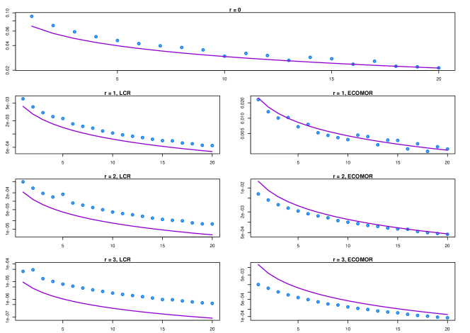
Figure 1: Numerical results for both LCR and ECOMOR treaties, for $a=20$.

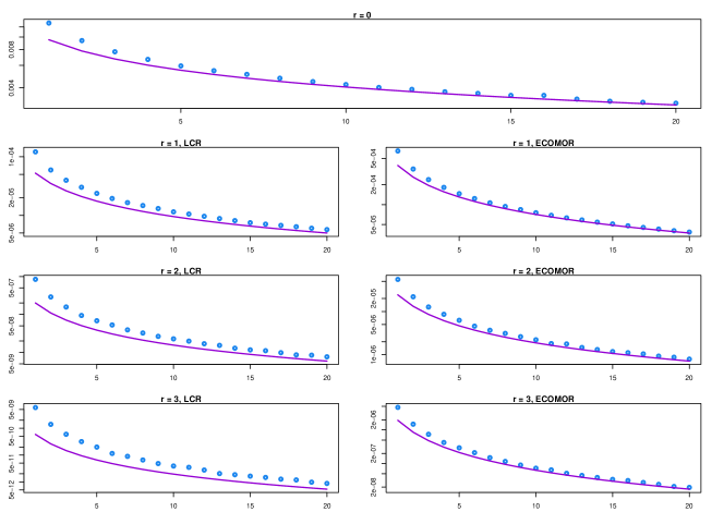
Figure 2: Numerical results for both LCR and ECOMOR treaties, for $a=80$.

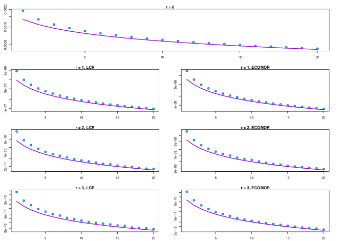
Figure 3: Numerical results for both LCR and ECOMOR treaties, for $a=300$.

Appendix A Appendix: Short description of the simulation technique

Our simulation estimator is based on an importance sampling strategy; see e.g. Chapter V of [5]. To be precise, for $\delta>0$, we define the auxiliary set

$$B_{\delta}=\{\xi\in\mathds{D}\colon\mathcal{D}(\xi,\delta)\geq r+1\},$$

where $\mathcal{D}(\xi,\delta)$ is given in (17). We propose an importance distribution $\mathds{Q}_{\delta,w}$ that is determined by

$$\mathds{Q}_{\delta,w}(\,\bullet\,)=w\mathds{P}(\,\bullet\,)+(1-w)\mathds{Q}_{\delta}(\,\bullet\,),$$

where $w\in(0,1)$ and $\mathds{Q}_{\delta}(\,\bullet\,)=\mathds{P}(\,\bullet\,|\,\bar{S}_{n}\in B_{\delta})$. Note that $\mathds{Q}_{\delta}(\,\bullet\,)$ is the conditional distribution given the event $\bar{S}_{n}$ has at least $r+1$ discontinuities of magnitude $\delta$. The proposed importance distribution has the following interpretation. We flip a coin at the beginning of each simulation. We generate with probability $w$ the sample path of $\bar{S}_{n}$ under the original measure and with probability $1-w$, we sample $\bar{S}_{n}$ under the measure $\mathds{Q}_{\delta}(\,\bullet\,)$. To compensate for the bias introduced by the importance distribution, a likelihood ratio – that is the Radon/Nikodym derivative between $\mathds{P}$ and $\mathds{Q}_{\delta,w}$ – must be included in the estimator. In our case, the estimator $Z_{n}$ for $\mathds{P}(\bar{S}_{n}\in A)$ is then given by

$$Z_{n}=\mathds{1}_{\{\bar{S}_{n}\in A\}}\frac{d\mathds{P}}{d\mathds{Q}_{\delta,w}}=\mathds{1}_{\{\bar{S}_{n}\in A\}}\left(w+\frac{1-w}{\mathds{P}(\bar{S}_{n}\in B_{\delta})}\mathds{1}_{\{\bar{S}_{n}\in B_{\delta}\}}\right)^{-1}.$$

The output analysis is performed similarly to the Monte Carlo method, i.e. we generate $M$ i.i.d. replicates of $Z_{n}$ from $\mathds{Q}_{\delta,w}$ and we estimate $\mathds{P}(\bar{S}_{n}\in A)$ as the arithmentic mean of the replicates. From Theorem 1 in [9], there exists $\delta$ such that the simulation estimator has a bounded relative error. Hence, the number of simulation runs required to achieve a given accuracy is bounded as $n$ goes to infinity. For more details of the estimator, we refer the readers to [9].

References

- [1] H. Albrecher, C. Robert, and J. Teugels. Joint asymptotic distributions of smallest and largest insurance claims. Risks, 2(3):289–314, 2014.
- [2] H. Albrecher, J. L. Teugels, and J. Beirlant. Reinsurance: Actuarial and Statistical Aspects. John Wiley & Sons, 2017.
- [3] H. Ammeter. The rating of “Largest Claim” reinsurance covers. Quarterly letter from the Algemeene Reinsurance Companies Jubilee, (2):5–17, 1964.
- [4] S. Asmussen and H. Albrecher. Ruin Probabilities. Advanced Series on Statistical Science & Applied Probability, 14. World Scientific, Second edition, 2010.
- [5] S. Asmussen and P. Glynn. Stochastic Simulation: Algorithms and Analysis, volume 57 of Stochastic Modelling and Applied Probability. Springer-Verlag New York, 2007.
- [6] S. Asmussen and C. Klüppelberg. Large deviations results for subexponential tails, with applications to insurance risk. Stochastic processes and their applications, 64(1):103–125, 1996.
- [7] B. Berliner. Correlations between excess of loss reinsurance covers and reinsurance of the largest claims. ASTIN Bulletin: The Journal of the IAA, 6(3):260–275, 1972.
- [8] A. Castaño-Martìnez, G. Pigueiras, and M. Sordo. On a family of risk measures based on largest claims. Insurance: Mathematics and Economics, 2019.
- [9] B. Chen, J. Blanchet, C.-H. Rhee, and B. Zwart. Efficient rare-event simulation for multiple jump events in regularly varying random walks and compound poisson processes. arXiv:1706.03981v1.
- [10] P. Embrechts, C. M. Goldie, and N. Veraverbeke. Subexponentiality and infinite divisibility. Probability Theory and Related Fields, 49(3):335–347, 1979.
- [11] P. Embrechts, C. Klüppelberg, and T. Mikosch. Modelling Extremal Events: for Insurance and Finance, volume 33 of Applications of Mathematics. Springer-Verlag, 1997.
- [12] E. Hashorva and J. Li. Ecomor and lcr reinsurance with gamma-like claims. Insurance: Mathematics and Economics, 53(1):206–215, 2013.
- [13] J. Jiang and Q. Tang. Reinsurance under the lcr and ecomor treaties with emphasis on light-tailed claims. Insurance: Mathematics and Economics, 43(3):431–436, 2008.
- [14] A. E. Kyprianou. Introductory Lectures on Fluctuations of Lévy Processes with Applications. Universitext. Springer-Verlag, Berlin, 2006.
- [15] S. A. Ladoucette and J. L. Teugels. Reinsurance of large claims. Journal of Computational and Applied Mathematics, 186(1):163–190, 2006.
- [16] J. Li. Asymptotics for large claims reinsurance in a time-dependent renewal risk model. Scandinavian Actuarial Journal, 2015(2):172–183, 2015.
- [17] L. Peng. Joint tail of ecomor and lcr reinsurance treaties. Insurance: Mathematics and Economics, 58:116–120, 2014.
- [18] C.-H. Rhee, J. Blanchet, and B. Zwart. Sample path large deviations for lévy processes and random walks with regularly varying increments. arXiv: 1606.02795v3.
- [19] A. Thépaut. Une nouvelle forme de réassurance: Le traité d’excédent du coût moyen relatif (ecomor). Bulletin Trimestriel de l’Institut des Actuaires Français, (49):273–343, 1950.
- [20] W. Whitt. Stochastic-Process Limits: An introduction to stochastic-process limits and their application to queues. Springer Series in Operations Research. Springer-Verlag, 2002.