Observation of a new structure near $10.75\,\mathrm{GeV}$ in the energy dependence of the $e^{+}e^{-}\to\Upsilon(nS)\pi^{+}\pi^{-}$ ($n=1,2,3$) cross sections

Abstract

We report a new measurement of the $e^{+}e^{-}\to\Upsilon(nS)\pi^{+}\pi^{-}$ ($n=1,2,3$) cross sections at energies from $10.52$ to $11.02\,\mathrm{GeV}$ using data collected with the Belle detector at the KEKB asymmetric-energy $e^{+}e^{-}$ collider. We observe a new structure in the energy dependence of the cross sections; if described by a Breit-Wigner function its mass and width are found to be $M=(10752.7\pm 5.9\,^{+0.7}_{-1.1})\,\mathrm{MeV}/c^{2}$ and $\Gamma=(35.5^{+17.6}_{-11.3}\,{}^{+3.9}_{-3.3})\,\mathrm{MeV}$, where the first error is statistical and the second is systematic. The global significance of the new structure including systematic uncertainty is 5.2 standard deviations. We also find evidence for the $e^{+}e^{-}\to\Upsilon(1S)\pi^{+}\pi^{-}$ process at the energy $10.52\,\mathrm{GeV}$, which is below the $B\bar{B}$ threshold.

1 Introduction

The observed vector bottomonium states above the $B\bar{B}$ threshold, $\Upsilon(4S)$, $\Upsilon(10860)$, and $\Upsilon(11020)$, have properties that are unexpected for pure $b\bar{b}$ bound states Bondar:2016hva . Their transitions to lower bottomonia with the emission of light hadrons have much higher rates compared to expectations for ordinary bottomonium, and some of these transitions strongly violate Heavy Quark Spin Symmetry. A possible explanation of these unusual properties is a contribution of hadron loops or, equivalently, the presence of a $B_{(s)}^{(*)}\bar{B}_{(s)}^{(*)}$ admixture in the bottomonium wave function Meng:2007tk ; Simonov:2008ci ; Voloshin:2012dk . In this approach, the $\Upsilon(10860)$ and $\Upsilon(11020)$ are the $\Upsilon(5S)$ and $\Upsilon(6S)$ states “dressed” by hadrons.

In the region of the $\Upsilon(4S,5S,6S)$ states, quark models also predict the $\Upsilon(3D,4D)$ levels Ebert:2011jc ; Godfrey:2015dia . The electron widths of the $D$-wave states arise from mixing with the $S$-wave states, which is expected to be quite small for bottomonia below the $B\bar{B}$ threshold Moxhay:1983vu . However, it can be significantly enhanced for the states above open-flavor thresholds because of $B$-meson loops Badalian:2009bu . Thus, the “dressed” $\Upsilon(3D,4D)$ states might be formed abundantly in $e^{+}e^{-}$ annihilations.

The unexpected properties of the $\Upsilon(10860)$ and $\Upsilon(11020)$ could also be due to the presence of other exotic states, e.g., compact tetraquarks Ali:2009es or hadrobottomonia Dubynskiy:2008mq . To understand the nature of the already known $\Upsilon$ states above the $B\bar{B}$ threshold and to search for additional states expected in this energy region, it is of interest to study the energy dependence of the $e^{+}e^{-}\to(b\bar{b}...)$ cross sections, where $(b\bar{b}...)$ denotes exclusive final states containing the $b$ and $\bar{b}$ quarks, both with open and hidden flavor.

Recently, the Belle experiment measured the energy dependence of the cross sections $e^{+}e^{-}\to\Upsilon(nS)\pi^{+}\pi^{-}$ ($n=1,2,3$) Santel:2015qga , $e^{+}e^{-}\to h_{b}(nP)\pi^{+}\pi^{-}$ ($n=1,2$) Abdesselam:2015zza , $e^{+}e^{-}\to\chi_{bJ}(1P)\,\pi^{+}\pi^{-}\pi^{0}$ Yin:2018ojs , and $e^{+}e^{-}\to{B}_{s}^{(*)}\bar{B}_{s}^{(*)}$ Abdesselam:2016tbc in the energy region from 10.63 to $11.02\,\mathrm{GeV}$. The shapes of the $\Upsilon(nS)\pi^{+}\pi^{-}$ and $h_{b}(nP)\pi^{+}\pi^{-}$ cross sections show prominent $\Upsilon(10860)$ and $\Upsilon(11020)$ signals with no significant non-resonant contributions. Production of the $h_{b}(nP)\pi^{+}\pi^{-}$ is found to proceed entirely via the exotic charged bottomonium-like states $Z_{b}(10610)$ and $Z_{b}(10650)$ Belle:2011aa . The $B_{s}^{*}\bar{B}_{s}^{*}$ cross section shows a prominent $\Upsilon(10860)$ signal, while the $B_{s}\bar{B}_{s}$ and $B_{s}\bar{B}_{s}^{*}$ cross sections are relatively small and do not show any significant structures. The uncertainties in the $\chi_{bJ}(1P)\,\pi^{+}\pi^{-}\pi^{0}$ cross section at various energies are too large to draw conclusions about its shape. No evidence is found for new structures in any of these cross sections except possibly near $10.77\,\mathrm{GeV}$ in the $\Upsilon(nS)\pi^{+}\pi^{-}$ final states. It is of interest to study more channels and to improve the accuracy of the previously measured cross sections.

In this paper, we report an updated measurement of the $\sigma[e^{+}e^{-}\to\Upsilon(nS)\pi^{+}\pi^{-}]$ ($n=1,2,3$) energy dependence. We improve the accuracy by reconstructing $\Upsilon(nS)\to e^{+}e^{-}$ in addition to $\mu^{+}\mu^{-}$, and by extracting signal yields via fits to the $\pi^{+}\pi^{-}$ recoil mass distributions, instead of counting events with inverse efficiency weights in the signal and sideband regions, as was done previously Santel:2015qga . We also use the initial-state-radiation (ISR) process in the high statistics $\Upsilon(10860)$ on-resonance data to obtain additional information about the cross section shapes. As a result of these improvements, we observe a new structure in the energy dependence of the $e^{+}e^{-}\to\Upsilon(nS)\pi^{+}\pi^{-}$ ($n=1,2,3$) cross sections with a mass near $10.75\,\mathrm{GeV}$. We also find evidence for the $e^{+}e^{-}\to\Upsilon(1S)\pi^{+}\pi^{-}$ process below the $B\bar{B}$ threshold at $10.52\,\mathrm{GeV}$. This implies that the $e^{+}e^{-}\to\Upsilon(nS)\pi^{+}\pi^{-}$ cross sections have non-resonant contributions.

The paper is organized as follows. In Section 2 we present the data sets used in the analysis, and briefly describe the Belle detector and Monte-Carlo (MC) simulation. In Section 3 we list selection requirements for signal events. Section 4 is devoted to the center-of-mass (c.m.) energy calibration using the $e^{+}e^{-}\to\mu^{+}\mu^{-}$ process. In Section 5 we present an analytical calculation of the $e^{+}e^{-}\to\Upsilon(nS)\pi^{+}\pi^{-}$ signal shapes in the $M_{\rm recoil}(\pi^{+}\pi^{-})$ distributions and calibration of momentum resolution using the $\Upsilon(2S,3S)\to\Upsilon(1S,2S)\pi^{+}\pi^{-}$ transitions in the $\Upsilon(2S)$ and $\Upsilon(3S)$ data. Fits to the $M_{\rm recoil}(\pi^{+}\pi^{-})$ distributions are described in Section 6, while the results of the measurement of the Born cross sections and c.m. energy calibration using combined $e^{+}e^{-}\to\mu^{+}\mu^{-}$ and $e^{+}e^{-}\to\Upsilon(nS)\pi^{+}\pi^{-}$ processes are presented in Section 7. The fit to the cross section energy dependence, determination of the parameters of the intermediate states, and of the significance of the new structure are presented in Section 9. In Section 10 we give conclusions and mention possible interpretations of the new structure.

2 Data sets, Belle detector and simulation

The analysis is based on data collected by the Belle detector at the KEKB asymmetric-energy $e^{+}e^{-}$ collider BELLE_DETECTOR ; KEKB . We use energy scan data with approximately $1\,\mathrm{fb}^{-1}$ per point collected in the energy range from $10.63\,\mathrm{GeV}$ to $11.02\,\mathrm{GeV}$. These data were collected during two running periods, one with six energy points in 2007 and the other with sixteen energy points in 2010. We also use the $\Upsilon(10860)$ on-resonance data sample, with a total luminosity of $121\,\mathrm{fb}^{-1}$. These data were collected in five running periods with slightly different c.m. energies between $10.864\,\mathrm{GeV}$ and $10.868\,\mathrm{GeV}$. Finally, we use $60\,\mathrm{fb}^{-1}$ of the continuum data sample collected at $10.52\,\mathrm{GeV}$. Thus, in total, there are 28 energy points where we calibrate c.m. energies and measure cross sections. Energies and luminosities of various data samples are presented in Table 1.

The Belle detector is a large-solid-angle magnetic spectrometer that consists of a silicon vertex detector (SVD), a 50-layer central drift chamber (CDC), an array of aerogel threshold Cherenkov counters (ACC), a barrel-like arrangement of time-of-flight scintillation counters (TOF), and an electromagnetic calorimeter (ECL) comprised of CsI(Tl) crystals located inside a superconducting solenoid that provides a 1.5 T magnetic field. An iron flux return located outside the coil is instrumented to detect $K_{L}^{0}$ mesons and to identify muons (KLM). A more detailed description of the detector can be found in Ref. BELLE_DETECTOR .

The integrated luminosity is measured with barrel Bhabha events. The systematic error in the luminosity measurement is about 1.4% and is dominated by the theoretical uncertainty in the Bhabha cross section; the statistical error is usually small compared to the systematic error.

The detector response is simulated using GEANT GEANT . The MC simulation includes run-dependent variations in the detector performance and background conditions. The $e^{+}e^{-}\to\Upsilon(nS)\pi^{+}\pi^{-}$ ($n=1,2,3$) events including ISR are generated with EvtGen Lange:2001uf . We use matrix elements measured in the $\Upsilon(10860)$ on-resonance data Garmash:2014dhx . For the energy points outside the $\Upsilon(10860)$ peak, we use uniform Dalitz plot (DP) distributions to assess systematic uncertainty. The process $e^{+}e^{-}\to\mu^{+}\mu^{-}$ that is used in the c.m. energy calibration is simulated with Phokhara PHOKHARA . For the $\Upsilon(2S,3S)\to\Upsilon(2S,1S)\pi^{+}\pi^{-}$ transitions we use matrix elements measured by the CLEO experiment CroninHennessy:2007zz . Background from QED production of four-track final states is simulated using a specially developed extension of the BDK generator Krachkov:2019kty . Final-state radiation (FSR) is simulated with PHOTOS PHOTOS .

3 Event selection

We select events of the type $e^{+}e^{-}\to\Upsilon(nS)\pi^{+}\pi^{-}$ ($n=1,2,3$) with $\Upsilon(nS)\to\mu^{+}\mu^{-}$ or $e^{+}e^{-}$. A preselected sample containing $\mu^{+}\mu^{-}$ or $e^{+}e^{-}$ pairs with invariant masses greater than $8\,\mathrm{GeV}/c^{2}$ is used. Muons are identified by their range and transverse scattering in the KLM Abashian:2002bd . Electrons are identified by the presence of an ECL cluster matching a track in position and energy and having a transverse energy profile consistent with an electromagnetic shower; the ionization loss measurement in the CDC and the response of the ACC are also used Nakano:2002jw . We require the presence of two additional charged tracks that are identified as pions. Identification is based on the information from the TOF and ACC, combined with the ionization loss measurement in the CDC. We also apply an electron veto. The total efficiency of the identification requirements is at the level of 99% per pion. All tracks are required to originate from the interaction point (IP) region; this requirement helps eliminate poorly reconstructed tracks. Multiple candidates occur in about 0.5% of the events. We select the best candidate based on the smallest distance to IP in the plane transverse to the beam direction.

To suppress background from converted photons, we require $\cos\theta_{\pi^{+}\pi^{-}}<0.95$, where $\theta_{\pi^{+}\pi^{-}}$ is the pion opening angle in the laboratory frame. In the $e^{+}e^{-}\pi^{+}\pi^{-}$ final state we apply additional requirements, $M_{\mathrm{recoil}}(e^{+}e^{-})>350\,\mathrm{MeV}/c^{2}$ and $\cos\theta_{e^{-}}<0.82$, where $\theta_{e^{-}}$ is the angle between the $e^{-}$ momentum in the c.m. frame and the electron beam. The $e^{+}e^{-}$ recoil mass is defined as

$$M_{\rm recoil}(e^{+}e^{-})=\sqrt{(E_{\rm c.m.}-E_{e^{+}e^{-}})^{2}-p_{e^{+}e^{-}}^{\phantom{i}2}},$$ (1)

where $E_{\rm c.m.}$ is the c.m. energy, $E_{e^{+}e^{-}}$ and $p_{e^{+}e^{-}}$ are the $e^{+}e^{-}$ energy and momentum measured in the c.m. frame.

Figure 1 (left) shows the $M(\mu^{+}\mu^{-})$ vs. $M_{\rm recoil}(\pi^{+}\pi^{-})$ distribution for a high-statistics data sample (No. 9 in Table 1).

Figure 1: Left: $M(\mu^{+}\mu^{-})$ vs.  $M_{\rm recoil}(\pi^{+}\pi^{-})$ distribution in a high-statistics data sample (No. 9 in Table 1). Dashed lines show a diagonal band selected by the requirements of Eq. (2). Right: $M_{\rm recoil}(\pi^{+}\pi^{-})$ distributions for the selected $\mu^{+}\mu^{-}\pi^{+}\pi^{-}$ (top) and $e^{+}e^{-}\pi^{+}\pi^{-}$ (bottom) candidates. Results of the fit (red solid histogram) and background component of the fit function (black dotted histogram) are also shown.

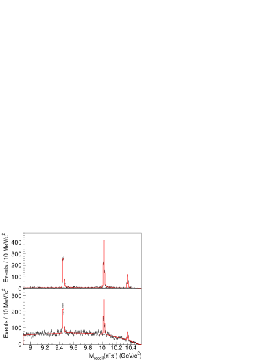
The clusters along the diagonal are due to $e^{+}e^{-}\to\Upsilon(nS)\pi^{+}\pi^{-}$ ($n=1,2,3$). Below the diagonal there are events in which some final-state particles are not reconstructed. The fully reconstructed events are selected with a requirement:

$$-150<M_{\rm recoil}(\pi^{+}\pi^{-})-M(\ell^{+}\ell^{-})<150\,\mathrm{MeV},$$ (2)

where $\ell=\mu$ or $e$. Since $M_{\rm recoil}(\pi^{+}\pi^{-})\approx E_{\rm c.m.}-E_{\pi^{+}\pi^{-}}$ and $M(\mu^{+}\mu^{-})\approx E_{\mu^{+}\mu^{-}}$, Eq. (2) corresponds to an energy balance requirement. The $M_{\rm recoil}(\pi^{+}\pi^{-})$ distributions are presented in Fig. 1 (right) for both $\mu^{+}\mu^{-}\pi^{+}\pi^{-}$ and $e^{+}e^{-}\pi^{+}\pi^{-}$ events.

4 Calibration of the center-of-mass energies with $e^{+}e^{-}\to\mu^{+}\mu^{-}$

In this section we describe the c.m. energy calibration with $e^{+}e^{-}\to\mu^{+}\mu^{-}$. Subsequently, the $E_{\rm c.m.}$ calibration is improved using the $e^{+}e^{-}\to\Upsilon(nS)\pi^{+}\pi^{-}$ ($n=1,2,3$) processes, as described in Section 6. For the $\Upsilon(10860)$ on-resonance data we use only $e^{+}e^{-}\to\Upsilon(nS)\pi^{+}\pi^{-}$.

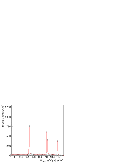
We select $e^{+}e^{-}\to\mu^{+}\mu^{-}$ events with the same requirements as described in Section 3 except requiring the presence of the $\pi^{+}\pi^{-}$ pair. We fit the $M(\mu^{+}\mu^{-})-E_{\rm c.m.}$ distributions for all data samples to a Gaussian in the range $\pm 70\,\mathrm{MeV}/c^{2}$ from the peak position, which corresponds to about $\pm 1\,\sigma$. Here and throughout the paper, we use a binned maximum-likelihood fit unless stated otherwise. An example of a fitted $M(\mu^{+}\mu^{-})$ distribution in the scan data sample is shown in Fig. 2.

Figure 2: $M(\mu^{+}\mu^{-})-E_{\rm c.m.}$ distribution for selected $e^{+}e^{-}\to\mu^{+}\mu^{-}$ candidates in the scan data sample. Red curve is the fit result.

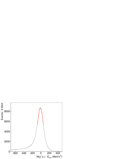
The statistical uncertainty in the peak position is typically $0.3\,\mathrm{MeV}/c^{2}$.

There is a difference between the $M(\mu^{+}\mu^{-})$ peak position and $E_{\rm c.m.}$ due to radiative effects. This difference is determined to be $-8.3\pm 0.6\,\mathrm{MeV}$ using the $e^{+}e^{-}\to\Upsilon(nS)\pi^{+}\pi^{-}$ processes in the $\Upsilon(10860)$ on-resonance data as described in Section 6. The error assigned is based on the scatter of the measurements in different on-resonance data samples; it corresponds to the uncertainty due to long-term stability of the detector performance. The dependence of the shift on $E_{\rm c.m.}$ is determined from MC simulation. The shift increases in absolute value by $0.3\,\mathrm{MeV}$ over the energy scan range $10.52-11.02\,\mathrm{GeV}$.

To estimate the systematic uncertainty in $E_{\rm c.m.}$, we vary the fit interval from $\pm 50\,\mathrm{MeV}/c^{2}$ to $\pm 80\,\mathrm{MeV}/c^{2}$ and take the largest deviation as an error; it is in the range $0.1-0.7\,\mathrm{MeV}$. We investigate the stability of the $K^{0}_{S}\to\pi^{+}\pi^{-}$ invariant mass over the data-taking period and assign a $1\,\mathrm{MeV}$ uncertainty due to a possible variation of the Belle solenoid magnetic field during energy scan. The overall uncertainty is determined as a quadrature sum of all contributions; the values are in the range $1.2-1.4\,\mathrm{MeV}$.

5 Signal density functions in the $M_{\rm recoil}(\pi^{+}\pi^{-})$ distributions

The c.m. energy calibration using the $e^{+}e^{-}\to\Upsilon(nS)\pi^{+}\pi^{-}$ ($n=1,2,3$) processes and the measurement of the corresponding yields is done by fitting the $\pi^{+}\pi^{-}$ recoil mass distributions. In this Section we describe the determination of signal density functions in the $M_{\rm recoil}(\pi^{+}\pi^{-})$ distributions, which is a key tool of this analysis.

The density functions for the $\Upsilon(nS)\pi^{+}\pi^{-}$ signals in the $M_{\rm recoil}(\pi^{+}\pi^{-})$ distributions are calculated as a sequence of convolutions that take into account the $\pi^{+}\pi^{-}$ momentum resolution, ISR, and the beam energy spread.

The momentum resolution function is a sum of a symmetric part and a tail on the high $M_{\rm recoil}(\pi^{+}\pi^{-})$ side due to FSR, decays in flight, and secondary interactions. The symmetric part is described by a sum of five Gaussians. Such a parameterization has enough flexibility to describe non-Gaussian tails and is fast to compute, which is crucial for performing convolutions. The sum of the first three Gaussians contains about 96% of the signal, its standard deviation is between $2\,\mathrm{MeV}/c^{2}$ and $4\,\mathrm{MeV}/c^{2}$ for various c.m. energies and channels. The FSR contribution is modeled with a photon energy threshold of $0.1\,\mathrm{MeV}$.

To calibrate the momentum resolution and to verify the simulation of its tails we use the high-statistics $\Upsilon(2S)\to\Upsilon(1S)\pi^{+}\pi^{-}$ signal in the $25\,\mathrm{fb}^{-1}$ data sample collected by Belle at the $\Upsilon(2S)$ peak. We use the same selection requirements as described in Section 3, with the upper boundary in Eq. (2) released to $250\,\mathrm{MeV}$. The $M_{\rm recoil}(\pi^{+}\pi^{-})-m(\Upsilon(1S))$ distribution is presented in Fig. 3. Due to the small total width of the $\Upsilon(2S)$ state, the contributions from the beam energy spread and ISR are negligibly small. Therefore we describe the signal by the momentum resolution function; its floated parameters are the normalization, the overall shift in $M_{\rm recoil}(\pi^{+}\pi^{-})$, and a scale factor $f$ for the width of the symmetric component (we multiply the $\sigma$ parameters of all Gaussians by $f$). The non-peaking background is parameterized with the threshold function

$$A\,(x-x_{0})^{p}\,e^{-c(x-x_{0})},$$ (3)

where $x=M_{\rm recoil}(\pi^{+}\pi^{-})$; $A$, $x_{0}$, $p$, and $c$ are parameters that are floated. We also consider the peaking backgrounds due to the $\Upsilon(2S)\to\Upsilon(1S)\eta$ transitions with $\eta\to\pi^{+}\pi^{-}\pi^{0}$ and $\pi^{+}\pi^{-}\gamma$. The shapes of these peaking backgrounds are determined from MC simulations and their normalizations are fixed relative to the signal. Fit results are presented in Fig. 3, which shows that the fit function describes the data well.

Figure 3: The $M_{\rm recoil}(\pi^{+}\pi^{-})-m(\Upsilon(1S))$ distribution for the data collected at the $\Upsilon(2S)$ resonance (points with error bars) and fit results (black solid histogram). Also shown are combinatorial background (cross-hatched histogram), background from $\eta$ decays (hatched histogram) and various contributions to the signal function: FSR with $\mathrm{E}_{\gamma}>0.1\,\mathrm{MeV}$ (blue dashed), decays in flight (magenta dotted) and secondary interactions (red dash-dotted). Both panels show the same distribution, but differ in bin sizes, linear or logarithmic scales of the vertical axes and ranges of the horizontal axes.

The value of $f$ is found to be

$$f=1.160\pm 0.003.$$ (4)

We have used $\Upsilon(3S)\to\Upsilon(1S,2S)\pi^{+}\pi^{-}$ transitions in the $3\,\mathrm{fb}^{-1}$ data sample collected at the $\Upsilon(3S)$, and find no indication of a dependence of $f$ on $\pi^{+}\pi^{-}$ energy. The shifts in $M_{\rm recoil}(\pi^{+}\pi^{-})$ are sensitive to the mass differences $m(\Upsilon(2S))-m(\Upsilon(1S))$, $m(\Upsilon(3S))-m(\Upsilon(1S))$, and $m(\Upsilon(3S))-m(\Upsilon(2S))$. For all transitions, we find that the shifts are consistent with zero; thus, no corrections to the recoil mass scale are applied.

For the ISR probability, we use a calculation to second order in $\alpha$ by Kuraev and Fadin Kuraev:1985hb . We multiply it by the relative change of the cross section with $\Delta E_{\rm c.m.}$, the shift in c.m. energy due to the emission of a photon, and by the relative change in the reconstruction efficiency. The efficiency slowly decreases with $\Delta E_{\rm c.m.}$ due to the $\pi^{+}\pi^{-}$ becoming softer. To convert from $\Delta E_{\rm c.m.}$ to $\Delta M_{\rm recoil}(\pi^{+}\pi^{-})$ we use the approximate relation $\Delta E_{\rm c.m.}=-\Delta M_{\rm recoil}(\pi^{+}\pi^{-})$. This approximation does not produce any visible effects in our analysis.

The contribution of the c.m. energy spread is modeled by a Gaussian multiplied by the cross section energy dependence. The $\sigma$ parameter of the Gaussian is found from a fit to the $e^{+}e^{-}\to\Upsilon(nS)\pi^{+}\pi^{-}$ ($n=1,2,3$) signals in the combined on-resonance data sample; this fit is described below. The measured value is

$$\sigma=5.36\pm 0.13\,\mathrm{MeV},$$ (5)

at the $\Upsilon(10860)$ on-resonance energy of $E_{\rm c.m.}=10.866\,\mathrm{GeV}$. To find the spread at other c.m. energies, we assume that it is proportional to $E_{\rm c.m.}$. We note that if the cross section changes rapidly with $E_{\rm c.m.}$, then, because of the energy spread, the average energy of the produced $\Upsilon(nS)\pi^{+}\pi^{-}$ combination is different from the average energy of the colliding beams. This can result in a shift of the visible peak position that is as large as a few $\mathrm{MeV}/c^{2}$.

After the momentum resolution, ISR and energy spread convolutions are performed, we multiply the resulting signal density function by the $\Delta M_{\rm recoil}(\pi^{+}\pi^{-})$ efficiency dependence of the energy balance requirement, which is a step function smeared by the $M(\mu^{+}\mu^{-})$ resolution, which is typically $\sigma=60\,\mathrm{MeV}/c^{2}$. The smearing is described with the error function.

The integrals of the momentum resolution and energy spread functions are normalized to unity; therefore the integral of the signal density function corresponds to that of the ISR function and the measured signal yield already includes the ISR correction, $1+\delta_{\mathrm{ISR}}$. Such a normalization of the signal function was used in Ref. Abdesselam:2015zza .

The calculation of the signal density function is performed inside the fit function that allows to float various parameters that influence the signal, such as the peak position, the c.m. energy spread, etc. The energy dependence of the cross section is required for the calculation of the signal density function; therefore the analysis is performed iteratively: we compute the signal density functions using results of the fit to the cross section energy dependence from the previous iteration.

6 Fits to $M_{\rm recoil}(\pi^{+}\pi^{-})$ distributions

To determine the $e^{+}e^{-}\to\Upsilon(nS)\pi^{+}\pi^{-}$ ($n=1,2,3$) signal yields and to calibrate the c.m. energies, we fit the $M_{\rm recoil}(\pi^{+}\pi^{-})$ distributions in different data samples. The $\mu^{+}\mu^{-}\pi^{+}\pi^{-}$ and $e^{+}e^{-}\pi^{+}\pi^{-}$ candidates are fitted simultaneously, while the fits in different data samples are independent. The fit function is the sum of the signal components, plus non-peaking and peaking backgrounds.

Signal density functions are calculated as described in Section 5. The yields in the $\mu^{+}\mu^{-}\pi^{+}\pi^{-}$ final state are floated, while the ratio of the yields in the $e^{+}e^{-}\pi^{+}\pi^{-}$ and $\mu^{+}\mu^{-}\pi^{+}\pi^{-}$ is fixed from MC simulation for all data samples except for the $\Upsilon(10860)$ on-resonance data. This latter sample is used to tune the MC simulation. The masses of the $\Upsilon(1S)$, $\Upsilon(2S)$ and $\Upsilon(3S)$ that enter the calculation of the signal density functions are floated with the constraints of their world average values Patrignani:2016xqp . We also introduce a common shift for all peaks, that represents a possible c.m. energy miscalibration. This common shift is floated without constraints for the on-resonance data and with the constraints from the $e^{+}e^{-}\to\mu^{+}\mu^{-}$ calibration for the scan and continuum data.

The $\mu^{+}\mu^{-}\pi^{+}\pi^{-}$ final-state background originates from the QED production of four tracks, e.g. two-photon $e^{+}e^{-}$ annihilations in which one virtual photon produces a high-mass $\mu^{+}\mu^{-}$ pair, and the other produces a $\pi^{+}\pi^{-}$, $\mu^{+}\mu^{-}$ or $e^{+}e^{-}$ pair, with the latter two misidentified as $\pi^{+}\pi^{-}$. There is a small peaking component in this type of processes due to the high-mass lepton pair being produced via the intermediate $\Upsilon(nS)$ ($n=1,2,3$). In case of the $e^{+}e^{-}\pi^{+}\pi^{-}$ final state there are also photon exchange diagrams and, thus, the background is higher.

The non-peaking component is described by an empirical function

$$B(x)=A\,(x-x_{0})^{p}\,P_{3}(x),$$ (6)

where $A$, $x_{0}$ and $p$ are parameters, $P_{3}(x)$ is a 3rd-order Chebyshev polynomial with a constant term set to unity. For high-statistics data samples all background parameters are floated. For low-statistics samples, only the normalization $A$ is floated, while the other parameters are fixed using the results of the fit to the combined on-resonance data sample; the threshold $x_{0}$ is recalculated for each of these data samples based on the energy of each sample. The peaking background is determined from MC simulation Krachkov:2019kty separately for each data sample. Its influence on the measured cross sections is found to be small.

In case of the lowest energy, $10.52\,\mathrm{GeV}$, reflections from the $\Upsilon(3S)\to\Upsilon(1S)\pi^{+}\pi^{-}$ and $\Upsilon(3S)\to\Upsilon(2S)\pi^{+}\pi^{-}$ transitions leak into the signal band in the $M(\mu^{+}\mu^{-})$ vs. $M_{\rm recoil}(\pi^{+}\pi^{-})$ plane due to the finite resolution of the $\mu^{+}\mu^{-}$ mass. The reflections are described in the fit by Gaussians with all parameters floated. Examples of the fits for the $\Upsilon(10860)$ on-resonance and scan data samples are shown in Figs. 1 and  4.

Figure 4: $M_{\rm recoil}(\pi^{+}\pi^{-})$ distributions in the data samples No. 4 (left) and 5 (right); the numbering is given in Table 1. Top and bottom panels correspond to $\mu^{+}\mu^{-}\pi^{+}\pi^{-}$ and $e^{+}e^{-}\pi^{+}\pi^{-}$ final states, respectively. Results of the fit (red solid histogram) and their background components (black dotted histogram) are also shown.

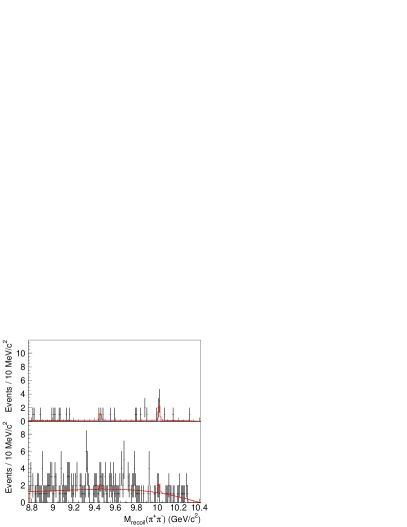
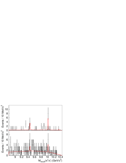
The $M_{\rm recoil}(\pi^{+}\pi^{-})$ spectra are fitted with $1\,\mathrm{MeV}/c^{2}$ bins, but we present them with larger bin sizes for clarity.

7 Results for the center-of-mass energies and the $\Upsilon(nS)\pi^{+}\pi^{-}$ cross sections

The calibrated c.m. energies are obtained from the fit results for the common shifts of the $\Upsilon(nS)\pi^{+}\pi^{-}$ signals. We do not find significant deviations from the constraints of the $e^{+}e^{-}\to\mu^{+}\mu^{-}$ calibration; the $e^{+}e^{-}\to\mu^{+}\mu^{-}$ and $e^{+}e^{-}\to\Upsilon(nS)\pi^{+}\pi^{-}$ energy calibrations agree well. The calibrated $E_{\rm c.m.}$ values are presented in Table 1.

No.	$E_{\rm c.m.}$	Luminosity	$\sigma(\Upsilon(1S)\pi^{+}\pi^{-})$	$\sigma(\Upsilon(2S)\pi^{+}\pi^{-})$	$\sigma(\Upsilon(3S)\pi^{+}\pi^{-})$
1	$10517.1\pm 1.4$	59.503	$0.040^{+0.021}_{-0.019}$	$0.025^{+0.029}_{-0.025}$	$-$
2	$10632.2\pm 1.5$	0.989	$0.21^{+0.23}_{-0.16}$	$-0.08^{+0.19}_{-0.04}$	$-$
3	$10681.0\pm 1.4$	0.949	$-0.08^{+0.08}_{-0.03}$	$0.06^{+0.27}_{-0.15}$	$-$
4	$10731.3\pm 1.5$	0.946	$0.34^{+0.33}_{-0.24}$	$0.93^{+0.49}_{-0.38}$	$-0.07^{+0.30}_{-0.08}$
5	$10771.2\pm 1.0$	0.955	$1.08^{+0.42}_{-0.35}$	$2.30^{+0.69}_{-0.59}$	$0.29^{+0.47}_{-0.24}$
6	$10829.5\pm 1.2$	1.172	$0.91^{+0.33}_{-0.28}$	$1.89^{+0.55}_{-0.47}$	$0.66^{+0.52}_{-0.38}$
7	$10848.9\pm 1.0$	0.989	$2.08^{+0.51}_{-0.45}$	$2.65^{+0.72}_{-0.62}$	$1.39^{+0.66}_{-0.52}$
8	$10857.4\pm 0.9$	0.988	$2.22^{+0.53}_{-0.47}$	$3.17^{+0.81}_{-0.72}$	$1.36^{+0.63}_{-0.50}$
9	$10864.2\pm 0.3$	47.647	$1.957^{+0.083}_{-0.080}$	$3.604^{+0.133}_{-0.131}$	$1.181^{+0.088}_{-0.084}$
10	$10865.8\pm 0.3$	24.238	$2.307^{+0.124}_{-0.121}$	$4.306^{+0.205}_{-0.199}$	$1.581^{+0.139}_{-0.131}$
11	$10865.9\pm 0.9$	1.814	$1.94^{+0.38}_{-0.34}$	$4.31^{+0.65}_{-0.60}$	$1.08^{+0.41}_{-0.34}$
12	$10867.5\pm 0.4$	21.368	$2.534^{+0.138}_{-0.133}$	$3.949^{+0.211}_{-0.205}$	$1.384^{+0.141}_{-0.133}$
13	$10867.7\pm 0.3$	22.938	$2.287^{+0.128}_{-0.124}$	$4.907^{+0.224}_{-0.218}$	$1.608^{+0.144}_{-0.137}$
14	$10867.9\pm 0.8$	0.978	$2.32^{+0.54}_{-0.48}$	$5.29^{+0.96}_{-0.86}$	$2.60^{+0.81}_{-0.68}$
15	$10877.8\pm 0.8$	0.978	$2.86^{+0.60}_{-0.54}$	$6.25^{+1.07}_{-0.97}$	$1.94^{+0.73}_{-0.60}$
16	$10882.8\pm 0.7$	1.278	$3.09^{+0.52}_{-0.47}$	$7.91^{+1.01}_{-0.94}$	$1.38^{+0.54}_{-0.45}$
17	$10888.9\pm 0.8$	0.990	$1.93^{+0.48}_{-0.42}$	$7.62^{+1.12}_{-1.04}$	$2.02^{+0.69}_{-0.58}$
18	$10898.3\pm 0.9$	0.983	$1.65^{+0.42}_{-0.37}$	$5.70^{+0.93}_{-0.85}$	$1.48^{+0.55}_{-0.45}$
19	$10898.3\pm 1.0$	0.883	$2.13^{+0.50}_{-0.44}$	$5.38^{+0.96}_{-0.87}$	$1.12^{+0.55}_{-0.43}$
20	$10907.3\pm 1.1$	0.980	$1.17^{+0.34}_{-0.29}$	$2.38^{+0.60}_{-0.53}$	$0.48^{+0.35}_{-0.25}$
21	$10928.7\pm 1.6$	0.680	$0.35^{+0.24}_{-0.19}$	$1.71^{+0.65}_{-0.52}$	$0.52^{+0.35}_{-0.26}$
22	$10957.5\pm 1.5$	0.855	$0.10^{+0.15}_{-0.10}$	$0.86^{+0.42}_{-0.35}$	$0.22^{+0.30}_{-0.22}$
23	$10975.3\pm 1.4$	0.999	$0.76^{+0.37}_{-0.31}$	$1.00^{+0.43}_{-0.35}$	$0.41^{+0.31}_{-0.23}$
24	$10990.4\pm 1.3$	0.985	$1.60^{+0.49}_{-0.42}$	$1.86^{+0.58}_{-0.49}$	$0.48^{+0.38}_{-0.27}$
25	$11003.9\pm 1.0$	0.976	$1.71^{+0.46}_{-0.41}$	$2.15^{+0.62}_{-0.54}$	$1.49^{+0.57}_{-0.49}$
26	$11014.8\pm 1.4$	0.771	$0.88^{+0.37}_{-0.31}$	$1.58^{+0.64}_{-0.54}$	$0.87^{+0.45}_{-0.35}$
27	$11018.5\pm 2.0$	0.859	$0.56^{+0.29}_{-0.23}$	$1.21^{+0.50}_{-0.42}$	$0.33^{+0.32}_{-0.23}$
28	$11020.8\pm 1.4$	0.982	$0.61^{+0.28}_{-0.23}$	$1.02^{+0.45}_{-0.38}$	$0.61^{+0.36}_{-0.28}$

Table 1: Calibrated c.m. energy (in GeV), luminosity of various data samples (in $\mathrm{fb}^{-1}$) and measured Born cross sections of the $e^{+}e^{-}\to\Upsilon(nS)\pi^{+}\pi^{-}$ ($n=1,2,3$) processes (in pb). The uncertainties in the energies and cross sections are totally uncorrelated.

Based on the measured signal yields we calculate Born cross sections:

$$\sigma^{B}=\frac{N\;|1-\Pi|^{2}}{\varepsilon\;L\;{\cal B}},$$ (7)

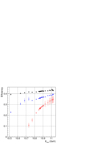
where $N$ is the signal yield (since the signal density function has been appropriately normalized, $N$ includes the ISR correction, as discussed in Section 5), $|1-\Pi|^{2}$ is a vacuum polarization correction taken from Ref. Actis:2010gg , $\varepsilon$ is the reconstruction efficiency (Fig. 5), $L$ is the integrated luminosity of each data sample (Table 1), and ${\cal B}$ is the branching fraction for $\Upsilon(nS)\to\mu^{+}\mu^{-}$ Patrignani:2016xqp .

Figure 5: Reconstruction efficiency as a function of the c.m. energy for the $\Upsilon(1S)\pi^{+}\pi^{-}$ (black filled dots), $\Upsilon(2S)\pi^{+}\pi^{-}$ (blue triangles), and $\Upsilon(3S)\pi^{+}\pi^{-}$ (red open dots) channels. The error bars show the systematic uncertainties associated with the DP model.

Measured $e^{+}e^{-}\to\Upsilon(nS)\pi^{+}\pi^{-}$ cross sections are presented in Table 1.

To study systematic uncertainties in $E_{\rm c.m.}$ and the cross sections, we vary the $E_{\rm c.m.}$ spread, the scale factor $f$, and the $e^{+}e^{-}\pi^{+}\pi^{-}$ to $\mu^{+}\mu^{-}\pi^{+}\pi^{-}$ efficiency ratio by $\pm 1\,\sigma$. We also increase the polynomial order in the background parameterization for high-luminosity data samples, while for low luminosity we release the coefficient of the linear term of the Chebyshev polynomial. Uncertainties associated with the cross section energy dependence are estimated using MC pseudoexperiments that are generated according to the fit results described in Section 9. The signal density functions are computed based on the fit results of each pseudoexperiment.

The systematic uncertainties are estimated based on the deviations of the measured quantities from their nominal values under the above variations of the analysis. In order to avoid overestimation of the relative uncertainties among the $\Upsilon(10860)$ on-resonance points, we separate uncertainties into correlated and uncorrelated parts. For each variation, we first find the average deviation over all the on-resonance points; this is used to estimate the correlated uncertainty. Then, we subtract the average deviation from deviations at each energy point. These relative deviations are used to estimate the uncorrelated uncertainties. In the case of the cross section energy dependence, we take the root mean squares of the deviations (for both correlated and uncorrelated parts). In all other cases, we take the maximal deviation as the uncertainty.

Uncertainties in efficiency associated with the DP model are treated as uncorrelated. The total uncorrelated systematic uncertainty is the sum in quadrature of all the contributions; dominant among them is the cross section energy dependence. The systematic uncertainty is small compared to the statistical uncertainty, as can be seen in Fig. 6. We add the two contributions in quadrature to find the total uncorrelated uncertainty. The c.m. energies and Born cross sections with total uncorrelated uncertainties are presented in Table 1.

Figure 6: Born cross sections for $e^{+}e^{-}\to\Upsilon(nS)\pi^{+}\pi^{-}$ ($n=1,2,3$) with statistical (black) and uncorrelated systematic (red) uncertainties, measured for different c.m. energies.

The correlated systematic errors include the uncertainties in the efficiency due to possible differences between data and MC in track reconstruction (0.35% per high and 1% per low momentum tracks, which are muons and pions, respectively) and muon identification, and the uncertainties in the luminosity and the branching fractions for $\Upsilon(nS)\to\mu^{+}\mu^{-}$ decays. The summary of the correlated errors is presented in Table 2.

Table 2: The systematic uncertainties in the $e^{+}e^{-}\to\Upsilon(nS)\pi^{+}\pi^{-}$ ($n=1,2,3$) cross sections correlated among various energy points (in percent).

	$\Upsilon(1S)\pi^{+}\pi^{-}$	$\Upsilon(2S)\pi^{+}\pi^{-}$	$\Upsilon(3S)\pi^{+}\pi^{-}$
$E_{\rm c.m.}$ spread	0.2	0.2	0.4
Momentum resolution	0.3	0.1	0.1
Cross section energy dependence	0.4	0.9	0.8
Tracking	2.7	2.7	2.7
Muon identification	2	2	2
Luminosity	1.4	1.4	1.4
Branching fractions	2.0	8.8	9.6
Total	4.2	9.6	10.3

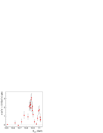
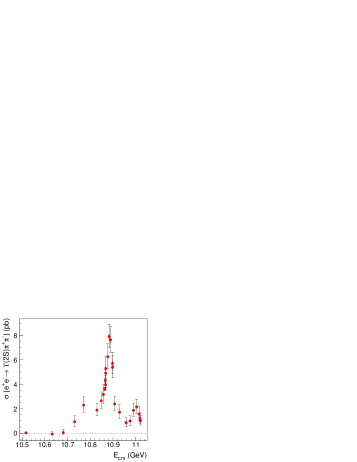
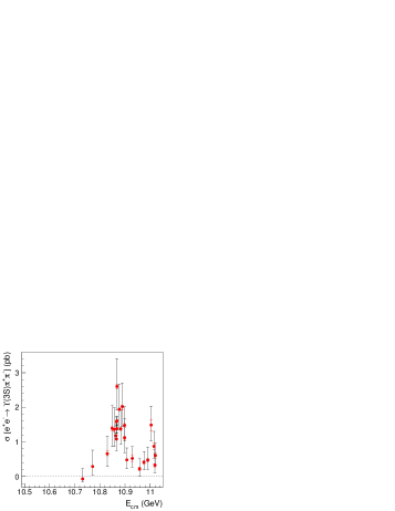
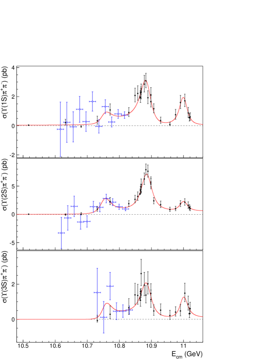
The energy-dependent cross sections (Fig. 6) show clear $\Upsilon(10860)$ and $\Upsilon(11020)$ peaks that were seen in previous publications Chen:2008xia ; Santel:2015qga . Due to the improved precision an additional structure around $E_{\rm c.m.}=10.75\,\mathrm{GeV}$, hinted at by the measurements in Ref. Santel:2015qga , is visible. The significance of this state is quantified in Section 9.

Recently, Belle studied the $e^{+}e^{-}\to\Upsilon(nS)\pi^{+}\pi^{-}$ ($n=1,2$) processes in the $\Upsilon(4S)$ on-resonance data Guido:2017cts and reported visible cross sections. For completeness, we include the corresponding Born cross sections here. We determine the $(1+\delta_{\mathrm{ISR}})$ factor to be $0.611\pm 0.011$, where the error includes uncertainty in the $\Upsilon(4S)$ parameters and uncertainty in the ISR photon energy cut-off. The Born cross sections at the $\Upsilon(4S)$ peak, recalculated based on the results of Ref. Guido:2017cts , are

$$\sigma(e^{+}e^{-}\to\Upsilon(1S)\pi^{+}\pi^{-}) =(0.1350\pm 0.0080\pm 0.0071)\,\mathrm{pb},$$ (8)

$$\sigma(e^{+}e^{-}\to\Upsilon(2S)\pi^{+}\pi^{-}) =(0.1293\pm 0.0134\pm 0.0132)\,\mathrm{pb}.$$ (9)

8 Study of the continuum data sample

In the continuum data sample at $E_{\rm c.m.}=10.52\,\mathrm{GeV}$, we find hints of non-zero values for the $\Upsilon(1S)\pi^{+}\pi^{-}$ and $\Upsilon(2S)\pi^{+}\pi^{-}$ cross sections, $40^{+21}_{-19}\,$fb and $25^{+29}_{-25}\,$fb, respectively. At this energy, contributions to the $\Upsilon(nS)\pi^{+}\pi^{-}$ cross sections due to $\Upsilon(4S)$, $\Upsilon(10860)$, or the new structure at $10.75\,\mathrm{GeV}$ are negligible (see next Section). To estimate the contributions of the $\Upsilon(2S)$ and $\Upsilon(3S)$ tails we use the Breit-Wigner function of Eq. (11) and world-average values for the $\Upsilon(1S,2S)$ masses, widths, electron widths and branching fractions Patrignani:2016xqp . We find 71 fb, 2 fb and 35 fb for the $\Upsilon(2S)\to\Upsilon(1S)\pi^{+}\pi^{-}$, $\Upsilon(3S)\to\Upsilon(1S)\pi^{+}\pi^{-}$, and $\Upsilon(3S)\to\Upsilon(2S)\pi^{+}\pi^{-}$ tails, respectively, which values are close to the experimental measurements.

The obtained expectations for the $\Upsilon(2S)\to\Upsilon(1S)\pi^{+}\pi^{-}$ and $\Upsilon(3S)\to\Upsilon(2S)\pi^{+}\pi^{-}$ tails are quite large because matrix elements of these three-body decays are dominated by the terms proportional to $M^{2}(\pi^{+}\pi^{-})$ (see, e.g., CroninHennessy:2007zz ). Corresponding partial widths are calculated as integrals of the matrix elements over phase space; they increase rapidly with the c.m. energy as high values of $M(\pi^{+}\pi^{-})$ become kinematically allowed. The dependence of the cross sections for various tails on $E_{\rm c.m.}$ is shown in Fig. 7.

Figure 7: Expected energy dependence of the cross sections for the processes $e^{+}e^{-}\to\Upsilon(2S)\to\Upsilon(1S)\pi^{+}\pi^{-}$ (solid blue), $e^{+}e^{-}\to\Upsilon(3S)\to\Upsilon(1S)\pi^{+}\pi^{-}$ (dashed black) and $e^{+}e^{-}\to\Upsilon(3S)\to\Upsilon(2S)\pi^{+}\pi^{-}$ (dotted red). These include the c.m. energy spread of $\sigma=5\,\mathrm{MeV}$.

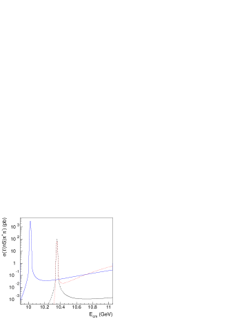
The cross sections start to increase above a certain energy. Uncertainties of the prediction of the tail contributions are discussed in the next Section.

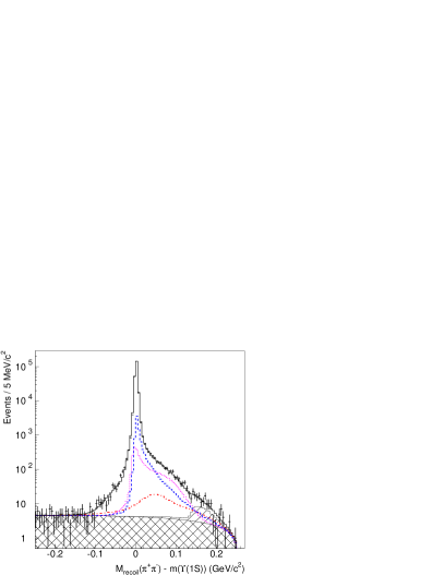
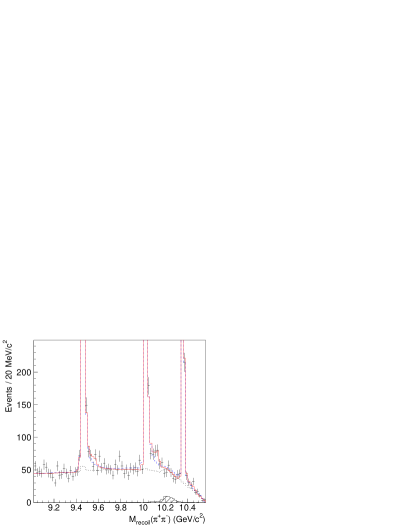
To verify the hypothesis of the $\Upsilon(2S,3S)$ tails, we note that the $M(\pi^{+}\pi^{-})$ distribution for the QED background is quite different from the expectations for the tails. The background is studied using the $\mu^{+}\mu^{-}\pi^{+}\pi^{-}$ events in the $\Upsilon(1S)$ sideband region $8.7<M_{\rm recoil}(\pi^{+}\pi^{-})<9.4\,\mathrm{GeV}/c^{2}$. The background $M(\pi^{+}\pi^{-})$ distribution (Fig. 8) is enhanced at low values and in the region of the $\rho$ meson; the MC simulation describes the shape and the normalization of the sideband data quite well.

Figure 8: The $M(\pi^{+}\pi^{-})$ distribution for the $\mu^{+}\mu^{-}\pi^{+}\pi^{-}$ events in the $\Upsilon(1S)$ sideband region $8.7<M_{\rm recoil}(\pi^{+}\pi^{-})<9.4\,\mathrm{GeV}/c^{2}$ at $E_{\rm c.m.}=10.52\,\mathrm{GeV}$. Points with error bars show data, the histograms show MC simulations of the total QED background (solid black) and various background components: $\mu^{+}\mu^{-}\pi^{+}\pi^{-}$ (dashed red), misidentified $4\mu$ (dotted blue), and misidentified $e^{+}e^{-}\mu^{+}\mu^{-}$ (dash-dotted green).

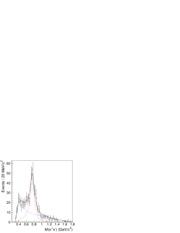
In contrast, the $\Upsilon(2S,3S)$ tail events are expected to concentrate near the upper kinematic boundary. To suppress the QED background, we apply a requirement $M(\pi^{+}\pi^{-})>0.85\,\mathrm{GeV}/c^{2}$, which is optimized using the figure of merit $\frac{S}{3/2+\sqrt{B}}$ Punzi:2004wh , where $S$ and $B$ are the number of signal and background events in the simulation, respectively. The $\pi^{+}\pi^{-}$ recoil mass distribution with this additional requirement for the $\mu^{+}\mu^{-}\pi^{+}\pi^{-}$ final state is shown in Fig. 9.

Figure 9: The $M_{\rm recoil}(\pi^{+}\pi^{-})$ distribution for $\mu^{+}\mu^{-}\pi^{+}\pi^{-}$ events with an additional requirement of $M(\pi^{+}\pi^{-})>0.85\,\mathrm{GeV}/c^{2}$ for the data sample at $E_{\rm c.m.}=10.52\,\mathrm{GeV}$. The peak at $9.63\,\mathrm{GeV}/c^{2}$ is due to the $\Upsilon(2S)\to\Upsilon(1S)\pi^{+}\pi^{-}$ transitions with ISR production of the $\Upsilon(2S)$. Result of the fit (red solid histogram) and the background component (black dotted histogram) are also shown.

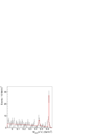
A clear signal for the $\Upsilon(1S)\pi^{+}\pi^{-}$ process is evident; its significance is estimated using Wilks’ theorem wilks to be $3.6\,\sigma$. The signal is stable against variations of the fit interval and the order of the polynomial used for the background parameterization. We conclude that the significance including systematic uncertainties is larger than $3.5\,\sigma$. The expected $M(\pi^{+}\pi^{-})$ requirement efficiency is 72% and is consistent with the reduction of the signal yield in the data. Based on the signal yield measured with the $M(\pi^{+}\pi^{-})$ requirement, we determine the $e^{+}e^{-}\to\Upsilon(nS)\pi^{+}\pi^{-}$ cross section at $E_{\rm c.m.}=10.52\,\mathrm{GeV}$ to be $0.042^{+0.017}_{-0.015}$ pb, where the uncertainties are statistical only. This result is model-dependent because of the unknown $M(\pi^{+}\pi^{-})$ distribution. In the fit to the cross section energy dependence, we use the value measured without the $M(\pi^{+}\pi^{-})$ requirement.

9 Fit to the energy dependence of the cross sections

Since the numbers of signal events in some scan data samples are small, the errors in the measured cross sections might be non-Gaussian. To address this issue, we scan $-2\ln\mathcal{L}$ of the $M_{\rm recoil}(\pi^{+}\pi^{-})$ fits in the signal yields. The $-2\ln\mathcal{L}$ dependence on the signal yield is then converted into the $-2\ln\mathcal{L}$ dependence on the cross section and is parameterized using an empirical function

$$f(x)=2\cdot(x\cdot p_{2}+p_{3}-p_{1}+p_{1}\ln\frac{p_{1}}{x\cdot p_{2}+p_{3}})\cdot P_{6}(x),$$ (10)

where $p_{1}$, $p_{2}$ and $p_{3}$ are fit parameters and $P_{6}$ is a 6th-order Chebyshev polynomial, with the zeroth-order parameter set to unity and all other parameters floated. To account for the systematic uncertainty, we convolve the distributions in $\mathcal{L}$ with Gaussian functions that represent uncorrelated systematic uncertainties. We find that there is good agreement between the scan results and the asymmetric Gaussian errors in the $\pm 1\,\sigma$ region; however, there are noticeable discrepancies for larger deviations. Therefore Gaussian errors should give a good approximation for a default fit that describes data well; while the $-2\ln\mathcal{L}$ scan results are important for significance calculation, in which case some points deviate from the alternative fit function by several standard deviations. In the fits to the cross section energy dependence, we use the $-2\ln\mathcal{L}$ scan results for all scan data points outside the $\Upsilon(10860)$ peak (points 2 to 8 and 20 to 28 in Table 1).

The ISR tails of the $\Upsilon(nS)\pi^{+}\pi^{-}$ signals in the $\Upsilon(10860)$ on-resonance data are sensitive to the cross section shapes in the region of the new structure at $10.75\,\mathrm{GeV}$. Therefore we include the $M_{\rm recoil}(\pi^{+}\pi^{-})$ distribution for the $\mu^{+}\mu^{-}\pi^{+}\pi^{-}$ final state, where background is lower, into the fit of the cross section energy dependence. Thus we perform a simultaneous fit to the $\Upsilon(nS)\pi^{+}\pi^{-}$ ($n=1,2,3$) cross sections and the $M_{\rm recoil}(\pi^{+}\pi^{-})$ distribution.

To parameterize the cross sections energy dependence, we consider contributions from the $\Upsilon(10860)$ and $\Upsilon(11020)$ resonances, the new structure, and the $\Upsilon(2S,3S)$ tails. Each contribution is represented by a Breit-Wigner amplitude:

$$F_{BW}(s,M,\Gamma,\Gamma_{ee}^{0}\times\mathcal{B}_{f})=\frac{\sqrt{12\pi\;\Gamma\;\Gamma_{ee}^{0}\times\mathcal{B}_{f}}}{s-M^{2}+iM\Gamma}\,\sqrt{\frac{\Gamma_{f}(s)}{\Gamma_{f}(M^{2})}},$$ (11)

where $M$ and $\Gamma$ are the mass and total width, $\Gamma_{ee}^{0}$ is the “bare” electron width related to the physical width by $\Gamma_{ee}^{0}=\Gamma_{ee}\,|1-\Pi(s)|^{2}$, and $\mathcal{B}_{f}$ and $\Gamma_{f}(s)$ are branching fraction and energy-dependent partial width of the decay to the $\Upsilon(nS)\pi^{+}\pi^{-}$ final state. The values of $\Gamma_{f}(s)$ at various energies are computed numerically by integrating the three-body decay matrix element over the DPs.

The new structure might have either resonant or non-resonant origin. In some cases, non-resonant effects produce peaks and have phase motion similar to resonances, as discussed, e.g., in Ref. Bugg:2011jr . Thus, we use the Breit-Wigner parameterization for the new structure amplitude.

In the default model the DP distributions of the $\Upsilon(10860)$, $\Upsilon(11020)$, and new structure decays are assumed to be the same, thus their amplitudes are added coherently. For the $\Upsilon(2S)\to\Upsilon(1S)\pi^{+}\pi^{-}$ and $\Upsilon(3S)\to\Upsilon(2S)\pi^{+}\pi^{-}$ tails we use the three-body matrix elements measured by CLEO CroninHennessy:2007zz . The interference terms between the tails and the rest of the amplitude are multiplied by “decoherence factors” that are calculated as overlap integrals of the DP matrix elements Santel:2015qga ; Abdesselam:2015zza , and can take values that range from 0 (incoherence) to 1 (full coherence). The values of the decoherence factors are found to be typically 0.7–0.8.

Complex phases of the $\Upsilon(11020)$, the new structure, and the $\Upsilon(2S,3S)$ amplitudes relative to the $\Upsilon(10860)$ amplitude are all floated in the fit individually for the three channels. We also float the $M$, $\Gamma$ and $\Gamma_{ee}^{0}\times\mathcal{B}_{f}$ parameters of the Breit-Wigner amplitudes except for $M$ and $\Gamma$ of the $\Upsilon(2S)$ and $\Upsilon(3S)$. The fit function to the $\Upsilon(nS)\pi^{+}\pi^{-}$ cross section at each c.m. energy contains a convolution with a Gaussian to account for the energy spread. The fit function to the $M_{\rm recoil}(\pi^{+}\pi^{-})$ distribution is the same as described in Section 6.

The fit results are presented in Figs. 10 and 11.

Figure 10: Energy dependence of the $e^{+}e^{-}\to\Upsilon(nS)\pi^{+}\pi^{-}$ cross sections ($n=1,2,3$ from top to bottom). The points with error bars are data with combined statistical and uncorrelated systematic uncertainties; the curves are the results of the simultaneous fit to these distributions and the $M_{\rm recoil}(\pi^{+}\pi^{-})$ distribution in the on-resonance data (Fig. 11). Shown are the results of the default fit (red solid curve) and the fit with the new structure excluded in all channels (blue dotted curve). The hatched histograms and the points with error bars at their maxima show the $\Upsilon(4S)$ line shapes and the cross sections measured at the $\Upsilon(4S)$ peak in Ref. Guido:2017cts . These points are not used in the fit to the cross section energy dependence. Insets show a zoom of the low energy region, while right side panels show a zoom of the $\Upsilon(10860)$ on-resonance region.

Figure 11: The $M_{\rm recoil}(\pi^{+}\pi^{-})$ distribution for the $\mu^{+}\mu^{-}\pi^{+}\pi^{-}$ events in the $\Upsilon(10860)$ on-resonance data; the right panel is a zoom of the left panel. Histograms show the results of the simultaneous fit to this distribution and the energy dependence of the $e^{+}e^{-}\to\Upsilon(nS)\pi^{+}\pi^{-}$ ($n=1,2,3$) cross sections (Fig. 10). The red solid histogram corresponds to the default fit, while the blue dashed histogram in the right panel corresponds to the fit with the new structure excluded. The black dotted histogram shows the background component of the default fit, the hatched one – peaking background from $\eta$ decays.

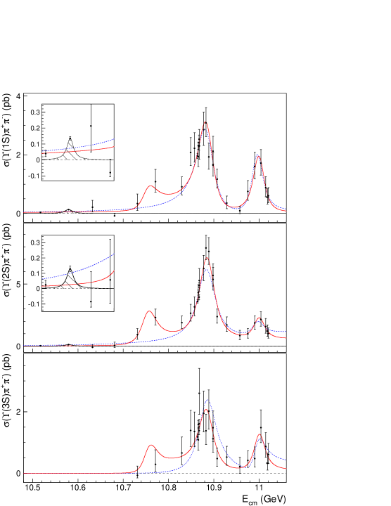
For illustration, we show in Fig. 10 the cross sections measured at the $\Upsilon(4S)$ peak and the expected $\Upsilon(4S)$ line shape; these measurements are not used in the fit. The fit results for masses and widths of the $\Upsilon(10860)$, $\Upsilon(11020)$, and new structure are presented in Table 3.

Table 3: Measured masses and widths of the $\Upsilon(10860)$, $\Upsilon(11020)$ and the new structure. The first uncertainty is statistical, the second is systematic.

	$\Upsilon(10860)$	$\Upsilon(11020)$	New structure
$\rm M\;(\mathrm{MeV}/c^{2})$	$10885.3\pm 1.5\,^{+2.2}_{-0.9}$	$11000.0^{+4.0}_{-4.5}\,{}^{+1.0}_{-1.3}$	$10752.7\pm 5.9\,^{+0.7}_{-1.1}$
$\Gamma\;(\mathrm{MeV})$	$36.6^{+4.5}_{-3.9}\,{}^{+0.5}_{-1.1}$	$23.8^{+8.0}_{-6.8}\,{}^{+0.7}_{-1.8}$	$35.5^{+17.6}_{-11.3}\,{}^{+3.9}_{-3.3}$

The results are slightly shifted from the previous Belle measurements based on the same data sample Santel:2015qga because we updated the cross section values at each energy, we fit now Born cross sections instead of visible ones, the new structure and the non-resonant contributions, i.e. the $\Upsilon(2S,3S)$ tails, are included in the fit model, and the energy dependence of the $\Gamma_{f}$ is taken into account.

A sum of several Breit-Wigner amplitudes produces multiple solutions that have the same values of $-2\ln L$, the same masses and widths, but different normalizations and relative phases. To search for multiple solutions, we create points with fitted values of the cross sections and small uncertainties. We then fit these points, one $\Upsilon(nS)\pi^{+}\pi^{-}$ channel at a time, repeating the fit many times with randomly generated initial values of the fit parameters. We find four or eight solutions in various channels, as expected for the sum of three or four Breit-Wigner amplitudes, respectively. The $\pm 1\,\sigma$ intervals of various solutions typically overlap, therefore we present only ranges in $\Gamma_{\rm ee}\times\mathcal{B}_{f}$ from the lowest to the highest solution (Table 4).

Table 4: The ranges of the $\Gamma_{\rm ee}\times\mathcal{B}$ values from the multiple solutions (in $\mathrm{eV}$).

	$\Upsilon(10860)$	$\Upsilon(11020)$	new
$\Upsilon(1S)\pi^{+}\pi^{-}$	$0.75-1.43$	$0.38-0.54$	$0.12-0.47$
$\Upsilon(2S)\pi^{+}\pi^{-}$	$1.35-3.80$	$0.13-1.16$	$0.53-1.22$
$\Upsilon(3S)\pi^{+}\pi^{-}$	$0.43-1.03$	$0.17-0.49$	$0.21-0.26$

To estimate the significance of the new structure in a single $\Upsilon(nS)\pi^{+}\pi^{-}$ channel, we repeat the fit with the new structure excluded in that channel. The significance is found based on the change in the $-2\ln L$ of the fit using Wilks’ theorem. The values are 2.7 and 5.4 standard deviations (${\sigma}$) in the channels $\Upsilon(1S)\pi^{+}\pi^{-}$ and $\Upsilon(2S)\pi^{+}\pi^{-}$, respectively. Using large sample of MC pseudoexperiments, we find that Wilks’ theorem provides slightly conservative estimation in our case. This is related to the fact that the number of experimental points in the region of the new structure is quite limited.

We also estimate the significance for all three $\Upsilon(nS)\pi^{+}\pi^{-}$ channels combined by performing the fit with the new structure excluded in all channels simultaneously. The $-2\ln{L}$ difference between the default fit and the null hypothesis fit is 65.8, with the cross section scan results contributing 51.7 and recoil mass distribution contributing 14.1. This $-2\ln{L}$ difference corresponds to a local significance of $7.0\,\sigma$, estimated using Wilks’ theorem. The global significance is estimated using the method described in Ref. Vitells:2011da . We find that the p-value of the fluctuation increases by a factor 4.5 due to the “look-elsewhere effect”, and the resulting global significance is $6.8\,\sigma$.

To estimate systematic uncertainties in the $\Upsilon(10860)$, $\Upsilon(11020)$, and new structure parameters, we vary the fit procedure. As an alternative parameterization of the new structure amplitude we use the threshold function, Eq. (3). For its parameters we find $x_{0}\approx 10.73\,\mathrm{GeV}/c^{2}$, $p\approx 0.17$ and $c\approx-10\,(\mathrm{GeV}/c^{2})^{-1}$. The quality of this fit is comparable to the default fit, with $-2\ln L$ worse by 3.4. Such a parameterization represents a threshold-like contribution without variation of a complex phase with energy. It has no clear physical meaning and we use it to conservatively estimate systematic uncertainty in the $\Upsilon(10860)$ and $\Upsilon(11020)$ parameters.

We study the influence of thresholds on the line shape of the $\Upsilon(10860)$ resonance. We consider the thresholds in the region of the new structure that show strong coupling to the $\Upsilon(10860)$. These are $B\bar{B}^{*}\pi$, $B^{*}\bar{B}^{*}\pi$ and $B_{s}^{*}\bar{B}_{s}^{*}$ at $10.75\,\mathrm{GeV}$, $10.79\,\mathrm{GeV}$ and $10.83\,\mathrm{GeV}$, respectively. The $B_{s}^{*}\bar{B}_{s}^{*}$ channel is the only among the $B_{s}^{(*)}\bar{B}_{s}^{(*)}$ channels that shows a prominent $\Upsilon(10860)$ signal Abdesselam:2016tbc . Production of the $B\bar{B}^{*}\pi$ and $B^{*}\bar{B}^{*}\pi$ channels proceeds entirely via intermediate $Z_{b}(10610)\pi$ and $Z_{b}(10650)\pi$ states, respectively Garmash:2015rfd , while the $Z_{b}\pi$ channels show prominent $\Upsilon(10860)$ signals in the $h_{b}(nP)\pi^{+}\pi^{-}$ final state Abdesselam:2015zza . Thus we multiply the constant width $\Gamma$ by an energy-dependent factor

$$1-x-y\ +x\,(p_{1}/p_{1}^{(0)})^{3}+y\,(\frac{2}{3}\,p_{2}/p_{2}^{(0)}+\frac{1}{3}\,p_{3}/p_{3}^{(0)}),$$ (12)

where $p_{i}$ ($i=1,2,3$) are momenta in the $B_{s}^{*}\bar{B}_{s}^{*}$, $Z_{b}(10610)\pi$ and $Z_{b}(10650)\pi$ pairs, respectively, and superscript $(0)$ denotes momentum calculated for the nominal $\Upsilon(10860)$ mass. The factors $\frac{2}{3}$ and $\frac{1}{3}$ correspond approximately to the ratio of the $B\bar{B}^{*}\pi$ and $B^{*}\bar{B}^{*}\pi$ cross sections Garmash:2015rfd . We set the weights $x$ and $y$ to various values of 0, 0.2, 0.4, and 0.6 with the restriction $x+y\leq 0.8$. We find that by introducing the effect of the $Z_{b}\pi$ thresholds we always increase the significance of the new structure. The reason for this is that the thresholds suppress the lower mass tails of the $\Upsilon(10860)$ resonance, and this leads to worse description of data under the null hypothesis.

We consider the possibility that either the $\Upsilon(11020)$ or the new structure, or both of them have a uniform distribution over the DP instead of that of the $\Upsilon(10860)$ model. This influences the $\Gamma_{f}(s)$ dependence on energy and the decoherence factors. For the $\Upsilon(10860)-\Upsilon(11020)$ decoherence we find 0.53, 0.66, and 0.82 in the $\Upsilon(1S)\pi^{+}\pi^{-}$, $\Upsilon(2S)\pi^{+}\pi^{-}$ and $\Upsilon(3S)\pi^{+}\pi^{-}$ channels, respectively, while for the $\Upsilon(10860)-$new structure decoherence we find 0.44, 0.34, and 0.85.

In the default model the tails of the $\Upsilon(2S)\to\Upsilon(1S)\pi^{+}\pi^{-}$ and $\Upsilon(3S)\to\Upsilon(2S)\pi^{+}\pi^{-}$ transitions are calculated under an assumption that matrix elements of the three-body decays grow with $M(\pi^{+}\pi^{-})$ as $M^{2}(\pi^{+}\pi^{-})$. This growth can be damped due to the presence of some form factor related to details of the hadronization process Voloshin_priv . We consider a damping factor of the decay amplitude in the form

$$\frac{1}{1+\frac{M(\pi^{+}\pi^{-})^{2}}{\Lambda^{2}}}$$ (13)

with the parameter $\Lambda$ taking the values 1, 2 and $4\,\mathrm{GeV}$. The $\Gamma_{f}(s)$ dependence for the $\Upsilon(2S,3S)$ tails is recalculated for each value of $\Lambda$. In all cases we find that the significance of the new structure increases. Thus, the default model corresponds to the fastest possible growth of the $\Upsilon(2S,3S)$ tails with energy and this gives a conservative estimate of the significance. We note that another reason why the growth of the non-resonant contribution with the energy could be damped is the crossing of various open-flavor thresholds. The tail of the $\Upsilon(3S)$ resonance can also contribute to the $\Upsilon(3S)\pi^{+}\pi^{-}$ final state. Thus, we include it into the fit using the same parametrization as for the $\Upsilon(2S)\pi^{+}\pi^{-}$ channel. To calculate its energy dependence and decoherence factors we assume that corresponding distribution over DP is uniform.

The significance of the new structure in the $\Upsilon(3S)\pi^{+}\pi^{-}$ channel in the default model is $3.9\,\sigma$. The reason why it is so high is evident from Fig. 10 (lowest panel): in the absence of the new structure the description of the $\Upsilon(3S)\pi^{+}\pi^{-}$ data in the region of the $\Upsilon(10860)$ peak becomes very poor. Thus, the new structure increases flexibility of the fit function in the region of the $\Upsilon(10860)$ peak due to interference. Obviously, a similar effect of interference can be achieved with a non-resonant contribution instead of the new structure. Indeed, the significance of the new structure in the $\Upsilon(3S)\pi^{+}\pi^{-}$ channel drops to $0.6\,\sigma$ once the non-resonant contribution is added. The production threshold in the $\Upsilon(3S)\pi^{+}\pi^{-}$ channel is above the continuum energy of $10.52\,\mathrm{GeV}$, therefore the information about the non-resonant contribution is limited, and available data do not allow to study the interplay between the new structure and the non-resonant contribution.

We consider the maximum deviation of the result as a systematic uncertainty associated with a given source. The different contributions and the total uncertainty obtained as their quadrature sum are presented in Table 5.

Table 5: Systematic uncertainties in the mass and width (in $\mathrm{MeV}/c^{2}$ and $\mathrm{MeV}$, respectively) of the $\Upsilon(10860)$, $\Upsilon(11020)$ and new structure.

	$\rm M_{\Upsilon(10860)}$	$\Gamma_{\Upsilon(10860)}$	$\rm M_{\Upsilon(11020)}$	$\Gamma_{\Upsilon(11020)}$	$\rm M_{new}$	$\Gamma_{\rm new}$
$\Upsilon_{\mathrm{new}}$ parameterization	${}^{+0.0}_{-0.8}$	${}^{+0.0}_{-0.4}$	${}^{+0.0}_{-0.7}$	${}^{+0.0}_{-0.6}$	$-$	$-$
$\Upsilon(10860)$ parameterization	${}^{+2.2}_{-0.0}$	${}^{+0.5}_{-0.0}$	${}^{+0.3}_{-0.0}$	$\pm 0.0$	${}^{+0.0}_{-0.1}$	${}^{+0.0}_{-0.1}$
$\Upsilon_{\mathrm{new}}$, $\Upsilon(11020)$ DP models	${}^{+0.1}_{-0.4}$	$\pm 0.2$	${}^{+0.7}_{-0.8}$	${}^{+0.7}_{-0.5}$	${}^{+0.6}_{-0.0}$	${}^{+3.1}_{-0.6}$
$\Upsilon(2S,3S)$ tails	${}^{+0.2}_{-0.3}$	${}^{+0.0}_{-1.0}$	${}^{+0.6}_{-0.7}$	${}^{+0.0}_{-1.6}$	${}^{+0.4}_{-1.1}$	${}^{+2.3}_{-3.2}$
Total	${}^{+2.2}_{-0.9}$	${}^{+0.5}_{-1.1}$	${}^{+1.0}_{-1.3}$	${}^{+0.7}_{-1.8}$	${}^{+0.7}_{-1.1}$	${}^{+3.9}_{-3.3}$

We find that the significance of the new structure in the $\Upsilon(2S)\pi^{+}\pi^{-}$ channel and global significance combined over all channels remain above $5.1\,\sigma$ and $5.2\,\sigma$, respectively, for all the variations that were introduced to study systematic uncertainties. The lowest significances are reached when we include the non-resonant contribution into the $\Upsilon(3S)\pi^{+}\pi^{-}$ channel.

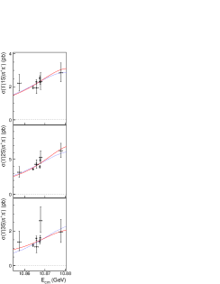
To visualize the ISR contribution to the measurement of the cross section energy dependence we estimate the $e^{+}e^{-}\to\Upsilon(nS)\pi^{+}\pi^{-}$ cross sections based on the ISR tails. For this, we divide the background-subtracted $M_{\rm recoil}(\pi^{+}\pi^{-})$ distributions in the ISR tail regions by the ISR luminosity function and efficiency, and apply other corrections from Eq. (7). Technically, to obtain the correction function we compute the $\Upsilon(nS)\pi^{+}\pi^{-}$ signal shape under an assumption that the cross section is constant with the c.m. energy and divide the obtained shape by the $\Upsilon(10860)$ on-resonance cross section. The results are presented in Fig. 12.

Figure 12: Energy dependence of the $e^{+}e^{-}\to\Upsilon(nS)\pi^{+}\pi^{-}$ cross sections ($n=1,2,3$ from top to bottom). Black points with error bars and red solid histograms are the same as in Fig. 10. Blue open dots with error bars are cross sections estimated using ISR process in the $\Upsilon(10860)$ on-resonance data. The blue dots are intended for visualisation only.

The cross sections estimated via ISR are compatible with the scan results and provide support for the new structure. However, they are not intended to be used in the fit, because the uncertainties are statistical only and do not include contributions due to the background subtraction. Also, the ISR luminosity changes rapidly in the studied energy region, which complicates accurate description of the resolution effects. It is only in the fit to the ISR tails in the $M_{\rm recoil}(\pi^{+}\pi^{-})$ distribution that all these issues are addressed rigorously.

All previous measurements of the $\Upsilon(4S)\to\Upsilon(1S,2S)\pi^{+}\pi^{-}$ branching fractions Guido:2017cts ; Sokolov:2009zy ; Aubert:2008az assume that the $e^{+}e^{-}\to\Upsilon(1S,2S)\pi^{+}\pi^{-}$ cross sections measured at the $\Upsilon(4S)$ are entirely due to $\Upsilon(4S)$ decays. To study the implications of the presence of non-resonant contributions, we include the $\Upsilon(4S)$ amplitude into the fit function and scan the $-2\ln L$ in the $\Upsilon(4S)$ branching fractions. The 67% confidence level intervals for $\mathcal{B}(\Upsilon(4S)\to\Upsilon(1S)\pi^{+}\pi^{-})$ and $\mathcal{B}(\Upsilon(4S)\to\Upsilon(2S)\pi^{+}\pi^{-})$ are found to be $(1.2-16)\times 10^{-5}$ and $(1.3-9.6)\times 10^{-5}$, respectively. The constraints on the branching fractions become weak because of interference between the $\Upsilon(4S)$ and the non-resonant amplitudes. We also find that introducing the $\Upsilon(4S)$ into the fit has a negligible effect on the measured mass and width values of the $\Upsilon(10860)$, $\Upsilon(11020)$, and new structure.

10 Conclusions

We report a new measurement of the energy dependence of the $e^{+}e^{-}\to\Upsilon(nS)\pi^{+}\pi^{-}$ ($n=1,2,3$) cross sections that supersedes the previous Belle result reported in Ref. Santel:2015qga . We observe a new structure in the energy dependence; if described by a Breit-Wigner amplitude, its mass and width are found to be $M=(10752.7\pm 5.9\,^{+0.7}_{-1.1})\,\mathrm{MeV}/c^{2}$ and $\Gamma=(35.5^{+17.6}_{-11.3}\,{}^{+3.9}_{-3.3})\,\mathrm{MeV}$. The global significance of the new structure including a systematic uncertainty is 5.2 standard deviations. We also report measurements of the $\Upsilon(10860)$ and $\Upsilon(11020)$ parameters with improved accuracy.

We find evidence for the $e^{+}e^{-}\to\Upsilon(1S)\pi^{+}\pi^{-}$ process at the energy $10.52\,\mathrm{GeV}$. Its cross section and the $M(\pi^{+}\pi^{-})$ distribution are consistent with the expectations for the $\Upsilon(2S)$ and $\Upsilon(3S)$ tails. Because of the presence of the non-resonant contributions, the $\Upsilon(4S)\to\Upsilon(1S,2S)\pi^{+}\pi^{-}$ branching fractions are poorly constrained by the available cross section measurements that are all performed at the $\Upsilon(4S)$ peak.

The new structure could have a resonant origin and correspond to a signal for the not yet observed $\Upsilon(3D)$ state provided $S-D$ mixing is enhanced Badalian:2009bu , or an exotic state, e.g. a compact tetraquark Ali:2009es or hadrobottomonium Dubynskiy:2008mq . It could also be a non-resonant effect due to some complicated rescattering. Information on the cross section energy dependence for more channels, with both hidden and open $b$ flavor, is needed to clarify the nature of the new structure.